
Using UAV LiDAR to Extract Vegetation Parameters of Inner Mongolian Grassland
by
 , ,
, ,
Xiang Zhang
1 ,
,
Yuhai Bao
1, 
Dongliang Wang
2,3,4,5,*,†,
Xiaoping Xin
3,†,
Lei Ding
3,
Dawei Xu
3,
Lulu Hou
3 and
Jie Shen
3 1
College of Geographic Science, Inner Mongolia Normal University, Hohhot 010022, China
2
Key Laboratory of Land Surface Pattern and Simulation, Institute of Geographic Sciences and Natural Resources Research, Chinese Academy of Science, Beijing 100101, China
3
Institute of Agricultural Resources and Regional Planning, Chinese Academy of Agricultural Sciences, Beijing 100081, China
4
State Key Laboratory of Resources and Environmental Information System, Institute of Geographic Sciences and Natural Resources Research, Chinese Academy of Sciences, Beijing 100101, China
5
Institute of UAV Application Research, Tianjin and CAS, Tianjin 301800, China
*
Author to whom correspondence should be addressed.
†
These authors contributed equally to this work.
Remote Sens. 2021, 13(4), 656; https://doi.org/10.3390/rs13040656
Submission received: 22 December 2020
/
Revised: 6 February 2021
/
Accepted: 8 February 2021
/
Published: 11 February 2021
(This article belongs to the Special Issue LiDAR for Precision Agriculture)
Abstract
:The accurate estimation of grassland vegetation parameters at a high spatial resolution is important for the sustainable management of grassland areas. Unmanned aerial vehicle (UAV) light detection and ranging (LiDAR) sensors with a single laser beam emission capability can rapidly detect grassland vegetation parameters, such as canopy height, fractional vegetation coverage (FVC) and aboveground biomass (AGB). However, there have been few reports on the ability to detect grassland vegetation parameters based on RIEGL VUX-1 UAV LiDAR (Riegl VUX-1) systems. In this paper, we investigated the ability of Riegl VUX-1 to model the AGB at a 0.1 m pixel resolution in the Hulun Buir grazing platform under different grazing intensities. The LiDAR-derived minimum, mean, and maximum canopy heights and FVC were used to estimate the AGB across the entire grazing platform. The flight height of the LiDAR-derived vegetation parameters was also analyzed. The following results were determined: (1) The Riegl VUX-1-derived AGB was predicted to range from 29 g/m2 to 563 g/m2 under different grazing conditions. (2) The LiDAR-derived maximum canopy height and FVC were the best predictors of grassland AGB (R2 = 0.54, root-mean-square error (RMSE) = 64.76 g/m2). (3) For different UAV flight altitudes from 40 m to 110 m, different flight heights showed no major effect on the derived canopy height. The LiDAR-derived canopy height decreased from 9.19 cm to 8.17 cm, and the standard deviation of the LiDAR-derived canopy height decreased from 3.31 cm to 2.35 cm with increasing UAV flight altitudes. These conclusions could be useful for estimating grasslands in smaller areas and serving as references for other remote sensing datasets for estimating grasslands in larger areas.

1. Introduction
Grasslands are an important part of the land surface ecosystem and account for approximately 27% of the global surface [1,2,3,4]. Grassland aboveground biomass (AGB) is a significant grassland productivity indicator informative for both engineers and grassland managers [5,6]. Moreover, AGB drives ecosystem processes via vegetation properties and biodiversity across multiple trophic levels in northern Sweden [7]. As one of the most important indices of grasslands, AGB can be used to evaluate carbon cycling and the net primary productivity for grasslands [8,9,10]. AGB can be effectively estimated using vegetation structure data, including canopy height and fractional vegetation coverage (FVC). FVC includes the ground layer (grasses, leaf litter, moss and lichen), mid layer (mid-sized trees, mid-storey cover) and canopy layer (hollow-bearing trees, canopy depth) as well as attributes capturing vegetation conditions (tree dieback, mistletoe) [11].
Traditional AGB field sampling efficiency is time consuming and costly. Biomass is traditionally measured by quadrats that were not defoliated by cutting or grazing during the growing season [12]. Although the data are accurate, data collection is time consuming, costly and laborious [13], and accurately acquiring grassland AGB data is difficult in larger areas. Passive optical remote sensing is an advanced grassland ecosystem monitoring tool in the management of grassland structure research on parameters such as vegetation coverage, AGB and vegetation growth [14,15,16]. L-band passive microwaves (1–2 GHz) have a strong ability to penetrate vegetation due to their long wavelength spectral range (15–30 cm) [17]. However, passive optical remote sensing suffers from saturation problems when estimating grassland biomass, especially in areas with high vegetation cover. The saturation problem of the vegetation index is characterized by lower accuracy in the vegetation index because the spectral bands (6–18 GHz) weakly penetrate through the vegetation layer compared with AGB accumulation when the grassland vegetation density reaches a certain threshold. In addition, UAV optical cameras have been used to improve the estimation accuracy of vegetation biomass-based structures from motion (SfM) algorithms and canopy height models (CHMs) [18]. In recent years, plant structure parameters (such as plant height) have become the focus of UAV-based remote sensing approaches for crop monitoring. The canopy surface model has a robust estimator of crop biomass. However, monitored arable crops typically suffer differences in floristic composition, and the co-occurrence of phenology leads to high spatial-temporal heterogeneity [19]. The emergence of this heterogeneity presents a great challenge for remote sensing to detect biomass. Electromagnetic radiation information received by remote sensing cannot accurately reflect a change in biomass, and remote sensing models cannot accurately estimate the distribution area of high biomass accumulation.
Light detection and ranging (LiDAR) acquires three-dimensional information (x, y, z) and emits a beam of light pulses, hits the object, and reflects it back; this information is ultimately received by the LiDAR sensor. Combined with a specified laser height and laser scanning angle, the laser position is obtained from global positioning systems and inertial navigation systems. As a method of 3D data acquisition, LiDAR technology has been widely used in agriculture [15,20], forestry [21,22,23] and many other industries [24,25]. LiDAR data offer a unique opportunity to measure three-dimensional vertical structures. For example, canopy height measurements rely on the laser pulse return from the vegetation and ground in different physical objects and different elevations. In recent years, unmanned aerial vehicle (UAV) LiDAR has also been used to monitor plant structures [26]. Owing to their low weight and cost, UAV LiDAR has been widely used in vegetation monitoring. Xiangqian Wu et al. [27] used a Velodyne LiDAR sensor to detect individual trees and estimate forests in China. Wang et al. [28] used Velodyne’s HDL-32E UAV LiDAR system to study the Hulun Buir grassland ecosystem. In summary, Velodyne’s LiDAR sensor can effectively extract vegetation parameters in forests and grasslands and rapidly evaluate AGB.
From the perspective of soil and ecology science, some researchers have carried out experiments on the Hulun Buir grazing platform to study the spatial distribution characteristics of soil carbon, nitrogen and grassland species under different grazing intensities [29,30,31]. However, there is still a lack of research on remote sensing detection of grassland vegetation on the Hulun Buir grazing platform. In this paper, we obtain RIEGL VUX-1 UAV LiDAR (Riegl VUX-1)-derived grassland vegetation structures to model the grassland AGB of the Hulun Buir grazing platform. This paper evaluates the ability of the Riegl VUX-1 sensor to extract grassland parameters. Using LiDAR data to obtain the canopy height, FVC and AGB prediction maps with a 0.1 m resolution under different grazing intensities are evaluated. We also analyze different flight heights of LiDAR-derived vegetation structures in the Hulun Buir grazing platform. The relevant conclusions can provide a theoretical reference for steppe grasslands under different grazing conditions in Inner Mongolia.
2. Materials and Methods
2.1. Study Area
The Hulun Buir grazing platform was established in 2009. The stocking rates were set to 0, 0.23, 0.34, 0.46, 0.69, and 0.92 AU ha−1, which are referred to as G0, G1, G2, G3, G4, and G5, respectively [32] (where 1 AU = 500 kg of adult cattle) (Figure 1). The area is located 8 km east of Hailaer, Inner Mongolia, China (49°20′24″ N, 119°59′44″ E). The area of each plot was 300 m × 160 m, and the total area was 90 hm2. In the Hulun Buir grazing platform area, the altitude is approximately 666–680 m, and the terrain slope is less than 3°. The average annual rainfall is between 350 mm and 400 mm, and approximately 80% of rainfall occurs during the growing season [28]. Grazing lasts approximately 120 days (from 1 June to 1 October) annually [33]. The vegetation characteristics in this area are those of typical steppe. The dominant vegetation species are Leymus chinensis, Stipa capillata, Carex pediformis, Filifolium sibiricum, Bupleurum scorzonerifolium, Galium verum and Pulsatilla turczaninovii.
First, we used TerraScan (Terrasolid Ltd., Helsinki, Finland) for module classification in the Terrasolid software package to preprocess the LiDAR data. LiDAR noise points were eliminated, and the LiDAR point cloud data were filtered and normalized. Second, we used LiDAR data divided into vegetation points, ground points and other points. The ground points were then used to generate a digital terrain model (DTM), and the vegetation points were then used to generate a digital surface model (DSM). The DSM minus DTM was gridded without interpolation to establish a canopy height model (CHM) with a 0.1 m spatial resolution. Third, we used LiDAR data to obtain the LiDAR-derived minimum canopy height, mean canopy height, maximum canopy height and FVC from CHM. Fourth, we analyzed a simple regression model between the LiDAR-derived vegetation structures (the minimum, mean and maximum canopy height and FVC) and ground-measured data with all training samples. Finally, we chose the best model to obtain grassland prediction maps at the plot scale in the grazing platform. The workflow is shown in Figure 2. The LiDAR workflow was similar to that in other studies [34,35] and is described below.
2.2. Ground Measurement Data Collection
Ground measurements started on 11 September 2018, with observations of the vegetation parameters (canopy height, FVC and AGB) of this steppe. As shown in Figure 2, six sample points were selected under each plot. Among them, we selected four ground-measured samples as model training samples, and two ground-measured samples were used as model validation samples. Ninety-six ground-measured 50 cm × 50 cm quadrats (in the W2 and W4 plots, the number of ground-measured samples was not sufficient; thus, these plots were not included in the model calculation) were established following a line transecting each plot [36].
The ground-measured grassland canopy height and FVC and AGB measurements were carried out in a 50 cm × 50 cm field quadrat. Nine measurement points were evenly selected throughout the quadrat. We recorded the mean, maximum and minimum values of the natural height of the grassland with a ruler. The FVC was ground-measured using an ordinary digital camera (Canon PowerShot G7 X, Tokyo, Japan). The manual threshold (10–30%) method was used to obtain vegetation pixels from camera red- and green-band images perpendicular to the ground at a height of 1 m. After identifying and counting the green vegetation pixels using these values [37], the AGB was then clipped at the ground level and dried at 65 °C for 48 h to a constant weight [30]. We also used the real-time kinematic product (RTK-G975, Beijing Hezhongsizhuang Technology Co., Ltd., Beijing, China). A reference station and mobile station were used to form the carrier phase, and the fixed RTK sites were used to obtain the geographic center coordinates of the 96 quadrats. The measurement accuracy was at the centimeter level, which was used to determine the central coordinate position of each quadrat.
2.3. LiDAR Data Collection
On 11 September 2018, we designed three UAV LiDAR flights for use in the study area. The UAV LiDAR data collected on the first and second flights covered 18 plots at a flight altitude of 119 m. With increasing flight altitude, the standard deviation of the LiDAR-derived canopy height decreased sharply [28]. The third UAV LiDAR flight was conducted over the W0 plot at heights of 40–110 m (at intervals of 10 m), and the flight speed was 8 m/s. Figure 3a shows the UAV flight lines.
The HS-600 UAV system adopts a DJI Matrice 600, and the weight of the HS-600 UAV system is 4.5 kg on the platform, which integrates a Riegl VUX-1 sensor with an AP15(X) inertial navigation system. As shown in Figure 3b, the Riegl VUX-1 sensor can provide a measurement rate of up to 500,000 pulses/s and a large field angle of view of 330°. The LiDAR data adopted the pulse ranging principle of the Riegl VUX-1 sensor through near-infrared laser beam scanning. The UAV flight parameters of the Riegl VUX-1 sensor are shown in Table 1.
2.4. LiDAR Data Analysis
LiDAR point data were mainly classified as vegetation, ground and other noise by the triangulated irregular network (TIN) filtering method [38], which is embedded in TerraScan (Terrasolid Ltd., Helsinki, Finland) for module classification in the Terrasolid software package to create a digital terrain model (DTM) and a digital surface model (DSM) from the LiDAR data. Classification points were assessed to ensure that most LiDAR points were correctly classified. The relative height LiDAR data were gridded without interpolation to establish a canopy height model (CHM) with a 0.1 m spatial resolution. To determine the CHM, some researchers compared the DSM at different vegetation growing season times with the initial DTM for the first measurement [39]. The CHM was defined as the difference between the DSM and DTM, which is expressed as follows:
To obtain a better match between the LiDAR-derived parameters and quadrat measurements, the side length of the window was set to 1.8 m in the interactive data language (IDL), which was slightly larger than the side length of the quadrat. The minimum canopy height derived from the LiDAR data corresponds to the quadrat with a centre coordinate position (i,j) [28] and is expressed as follows:
where indicates the LiDAR-derived minimum canopy height image pixel value , and is derived from the LiDAR image pixel value at centre coordinates of the CHM. Using the same method, and can be obtained as follows:
The FVC corresponding to the LiDAR data window with centre coordinates of (i,j) was calculated as the ratio of the LiDAR-derived canopy height pixel value (≥2 cm) to all CHM(i,j) pixel values and is expressed as follows [28]:
where indicates the number of canopy returns (we set the threshold to ≥2 cm) within , and indicates the number of all returns within .
The grassland model fitting degree R2 represents the correlation between the independent and dependent variables. The RMSE reflects the regression model error between the calculated and predicted values. A smaller RMSE value corresponds to a more precise regression model. The RMSE of the regression model was calculated from the 64 training samples and 32 validation samples. The R2 and RMSE values can be expressed as follows:
where n represents all validation samples, represents the ith ground-measured sample value, and represents the ith predicted sample value.
In multiple linear regression analysis, the results do not improve when additional independent variables are introduced because some values have a certain approximately linear or collinear relationship in remote-sensing information, resulting in strong correlations between multiple variables and easily causing data redundancy resulting in complex model calculations. To avoid the adverse effects of collinearity and correlation among multiple independent variables, this paper used Pearson correlation to filter the independent variables according to the needs of the data.
We used SPSS 19.0 software (IBM SPSS Statistics for Windows, Version 19.0. Armonk, NY: IBM Corp, USA), and Pearson correlation testing of the LiDAR-derived minimum, mean and maximum canopy heights and FVC of 64 training samples was carried out.
We validated the standard deviation (σ) of the LiDAR-derived canopy height in the W0 plot to analyze the influence of different flight heights ranging from 40 m to 110 m.
The symbol σ represents the standard deviation of the LiDAR-derived canopy height data and is defined as follows:
where represents LiDAR-derived canopy height pixel values, indicates the average LiDAR-derived canopy height value at the W0 plot, and is the number of all sampling points at the W0 plot.
3. Results
3.1. Ground-Matured Data Analysis
We used box plots to analyze the ground-measured data. Figure 4 shows the 96 ground-measurement quadrat data points. Ground-measured vegetation parameters showed a decreasing trend with increasing grazing intensity. Under the G0 grazing intensity, the ground-measured canopy height reached a maximum of 56.7 cm, the median canopy height was 45.61 cm, and the outlier value was 23.1 cm, while under the G5 grazing intensity, the outlier value was 6 cm, the median canopy height was 3.95 cm, and the minimum of the ground-measured canopy height was 2.5 cm. Under the G2 grazing intensity, the canopy height had a large box range. This conclusion indicates that the samples were scattered with large fluctuations ranging from 11.33 cm to 32.8 cm in canopy height. The maximum ground-measured FVC was 87.3%, and a large fluctuation ranged from 63.8% to 87.3% of FVC in the G3 subplot. The minimum ground-measured FVC was 48.7% in the G5 subplot. The maximum AGB was 443.4 g/m2 under the G0 grazing intensity. The median AGB in the G5 subplot was 96.18 g/m2, with a small fluctuation range from 62.6 g/m2 to 166.16 g/m2 of AGB.
3.2. LiDAR-Derived Vegetation Parameters
Using the LiDAR-derived results specified in Figure 5a,b, spatial distribution maps of the canopy height and FVC at the plot level using pixel data under different grazing intensities in the grazing platform were generated. Figure 5a,b shows that the LiDAR-derived canopy height and FVC at each subplot followed the expected order, with low grazing intensity observed for high vegetation. At the quantitative level, reduced grassland parameter values were associated with increased grazing intensity in each plot.
Figure 5c,d shows the LiDAR-derived grassland structures under different grazing intensities at the plot level. Under the G0 grazing intensity, the LiDAR-derived canopy height was 26.25 cm and the LiDAR-derived FVC was 78.69%. Under the G5 grazing intensity, the LiDAR-derived canopy height was 2.76 cm and the LiDAR-derived FVC was 62.27%. Additionally, the ground-measured canopy height and FVC based on 96 quadrats exhibited decreasing trends with increasing grazing intensity. The LiDAR-derived grassland parameter trends in all quadrats were associated with the ground-measured data.
3.3. Relationship between AGB and Canopy Height/FVC
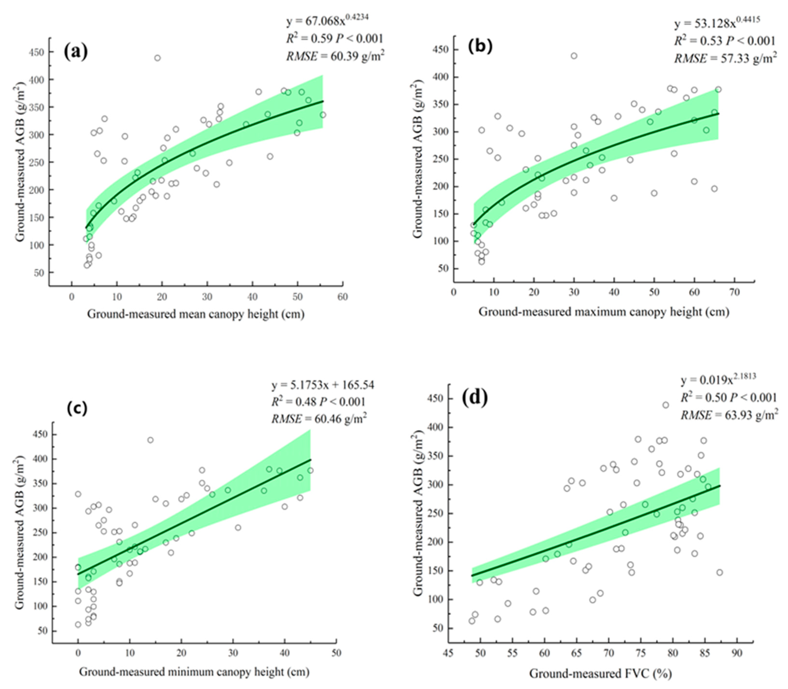
We analyzed all ground-measured grassland parameters for each quadrat, as displayed in Figure 6. We analyzed the relationship between the ground-measured canopy height, FVC and AGB. The correlation of all ground-measured data was statistically significant (p < 0001). Analysis of the ground-measured mean canopy height indicated a correlation with the AGB (R2 = 0.59, RMSE = 60.39 g/m2). The ground-measured maximum canopy height was correlated with the AGB (R2 = 0.53, RMSE = 57.33 g/m2). The minimum ground-measured canopy height showed the lowest correlation (R2 = 0.48, RMSE = 60.46 g/m2). The ground-measured FVC showed a correlation with R2 = 0.50 and RMSE = 63.93 g/m2. Thus, the results showed that grassland AGB can be better estimated using the ground-measured mean and maximum canopy heights and FVC.
The multiple linear regression results were also promising. Additionally, when the ground-measured maximum canopy height and FVC were combined, the AGB regression was slightly improved from R2 = 0.53 to R2 = 0.54 and RMSE = 57.33 g/m2 to RMSE = 55.79 g/m2. The results of the ground-measured analysis are similar to previous relevant conclusions [5,28]. This conclusion shows that there is a high correlation between canopy height and FVC, and the fitting degree estimating AGB from LiDAR data was limited because the ground-measured vegetation parameter data accuracy was higher than that of LiDAR-derived data. This conclusion also shows a weaker correlation between ground-measured AGB and LiDAR-derived vegetation parameters.
As shown in Figure 7, all LiDAR-derived canopy heights and FVC data points from the 64 training samples exhibited statistically significant correlations (p < 0.001) with the ground-measured parameters. However, the LiDAR data always underestimated the ground-measured canopy height and FVC. The LiDAR-derived canopy heights were approximately 1:3.26–1:1.13 as large as the ground-measured canopy heights, and the LiDAR-derived FVC was approximately 1:1.3 as large as the ground-measured FVC. Further research showed the fitting effects of the LiDAR-derived mean canopy height (R2 = 0.81, RMSE = 4.61 cm) and maximum canopy height (R2 = 0.92, RMSE = 3.61 cm). In terms of the FVC, the fitting effect was mainly between 75% and 85% (R2 = 0.51, RMSE = 4.89%), indicating that in most cases, the LiDAR-derived parameters underestimated the ground-measured vegetation parameters. Because of this correlation, the ground-measured data could be used to correct the LiDAR-derived canopy heights and FVC.
Due to the LiDAR signal penetrating the canopy, overlapping leaves appeared as a cluster in the image. If the vegetation was sparse and open, some LiDAR signals could pass through leaves and bounce back to the LiDAR. These openings appeared as holes in the image [40]. Analysis of LiDAR and ground-measured data revealed that the LiDAR-derived canopy height data were lower than the ground-measured data in the study area. There was a strong correlation between LiDAR and ground-measured data. In grassland ecosystems, ground-measured data can be used for calibration to improve the estimation accuracy of ground-measured canopy height and FVC. According to the analysis in Table 2, the LiDAR-derived vegetation parameters had significantly high levels of correlation (r > 0.6), and the lowest correlation coefficient (r = 0.62) was found between the LiDAR-derived mean canopy height and FVC. Therefore, we did not need to combine all LiDAR-derived canopy heights to calculate the grassland AGB.
3.4. LiDAR-Derived AGB
For the regression model analysis, we compared the LiDAR-derived canopy height and FVC to those of the grassland AGB model, and the results showed a statistically significant difference (p < 0.001) from the grassland AGB. A simple power-law regression model to predict the grassland AGB is suggested in Table 3, and the LiDAR-derived maximum canopy height and FVC were identified as prediction factors (R2 = 0.54, RMSE = 64.76 g/m2). Previous studies have established the power-law regression model as one of the most appropriate models. Because each grassland vegetation parameter can establish a relative growth model and exhibit heteroscedasticity phenomena in biomass models, it is better to build a power function model of independent variables or combined variables [41,42]. The regression model equation is as follows:
However, the AGB regression model resulted in almost no significant improvement in the grassland AGB model with only the LiDAR-derived canopy height. As shown in Table 3, the fitting degree of the LiDAR-derived maximum canopy height was better than that of the LiDAR-derived mean canopy height (R2 = 0.41–0.53, RMSE = 71.98–65.26 g/m2). After the FVC factor was added, the fitting effect of the power function model remained basically unchanged, and the RMSE generally declined, showing that adding the FVC effectively improved the model accuracy. Overall, the AGB model could be more effectively established by combining the power-law models of the canopy height and the FVC derived from the LiDAR point cloud data.
Using the results in Figure 5 and Table 3, the different LiDAR-derived regression models were evaluated using spatial distribution maps of the AGB with a 0.1 m spatial resolution. As shown in Figure 8a–c, low grazing intensity was observed for high AGB, while high grazing intensity was observed for low AGB.
Figure 8d–f shows the LiDAR-derived AGB under different grazing intensities at the plot level. The LiDAR-derived AGB showed a decreasing trend due to high grazing conditions. The LiDAR-derived grassland parameter trends in all quadrats were associated with the ground-measured data. However, overestimated or underestimated deviations may have been caused by topographic errors in the Riegl VUX-1 sensor. Overall, the Riegl VUX-1 sensor discrete-return LiDAR could distinguish grassland vegetation structures under different grazing conditions.
3.5. Analysis of the Flight Altitude
We also analyzed different flight altitudes (40–110 m) in the study area at the W0 subplot. In Figure 9, the analysis of flight height results shows that the LiDAR-derived canopy height exhibits a decreasing trend. The LiDAR-derived canopy height decreased from 9.19 cm to 8.17 cm, and the standard deviation of the LiDAR-derived canopy height decreased from 3.31 cm to 2.35 cm. However, the LiDAR-derived FVC showed an increasing trend with increasing flight height, and the LiDAR-derived FVC increased from 30.05% to 68.46%. The slowly decreasing LiDAR-derived canopy height results also showed that Riegl VUX-1 has high accuracy at a certain flight height. Therefore, more accurate data must be obtained, and we need to set a low flight altitude in the study area.
4. Discussion
We found that when estimating AGB based on the relevant vegetation index of ordinary optical images, saturation phenomenon easily occurs in the high vegetation coverage areas because ordinary optical images have difficulty detecting canopy height [43]. Based on the backscatter SAR sensor used to detect vegetation parameters, the change in signal wavelength was relatively weak, so it was difficult to accurately detect grassland canopy structure parameters and AGB [44,45]. Due to the characteristics of LiDAR data, three-dimensional canopy structure information can be directly obtained. The emergence of GEDI, ICESAT-2 and NISAR multisource sensor data fusion methods will contribute to the evaluation of AGB maps. Compared with other prediction maps, these maps have higher accuracy, more spatial coverage cover and higher spatial resolution [46,47].
All results show that UAV LiDAR data can estimate grassland AGB under different grazing intensities. The results also suggest that LiDAR-derived vegetation structures were well correlated with the ground-measured relative vegetation parameters (Figure 6). The LiDAR-derived maximum canopy height combined with the FVC showed the strongest correlation with the AGB and the highest accuracy (R2 = 0.54, RMSE = 64.76 g/m2) among the examined canopy structure indices. The analysis of LiDAR-derived parameters also showed that the improvement in the R2 values was limited after adding the LiDAR-derived FVC values, as shown in Table 3. The RMSE values decreased to 61.48–71.23 g/m2 when the LiDAR-derived canopy height and FVC were combined to calculate the grassland AGB. In recent years, some researchers have used LiDAR and optical image-based structure from motion (SfM) alternative 3D point cloud methods to improve model accuracy [48,49]. If we increase the amount of ground-measured sample data, we can use random forest and SfM algorithms to build a more advanced AGB model [50]. The accuracy and fitting effect of the model require further exploration.
We analyzed all LiDAR-derived vegetation parameters and found that all parameters showed strong correlations, as shown in Table 3 (r > 0.6). Other studies focusing on different vegetation species, including conifer/softwood or deciduous/hardwood forests, have also found similar relationships and conclusions [51,52,53]. Such a similar finding can be attributed to the capability of UAV LiDAR sensors to penetrate the grassland canopy at different flight heights. The main difference is underestimation under different UAV LiDAR densities and wavelengths [54,55]. Another influence on LiDAR-derived vegetation structures is the difference in flight heights [28]. Figure 9 shows that different flight altitudes influence the LiDAR-derived grassland parameters from 40 to 110 m. Different flight heights showed no major effect on the derived canopy height. These results are consistent with previous conclusions [56]. The slowly decreasing LiDAR-derived canopy height results also showed that Riegl VUX-1 exhibited a high accuracy for flight heights of 40 to 110 m. Therefore, more accurate data are needed at low flight altitudes (<40 m) in the study area. Further research is needed using the optimal flight height of 90–100 m for the Hulun Buir grassland with an FVC of ~65%. This result is similar to the results of ground-measured FVC in Hulun Buir grassland. This conclusion can be used to set the flight altitude of UAVs at 90–100 m to accurately and quickly calculate the Hulun Buir grassland FVC.
Different grazing intensities were also analyzed between LiDAR-derived vegetation structures and ground-measured data. Figure 6 shows that the LiDAR-derived canopy height and FVC distribution maps and values were consistent with the grazing intensities shown in Figure 2. Low grazing intensity was observed for high vegetation, and high grazing intensity was observed for low vegetation. The discrete-return Riegl VUX-1 is an advanced three-dimensional sensor that can estimate distribution maps under different grazing intensities. Previous scientists have been limited by severe saturation problems in optical images in grasslands with high vegetation cover when detecting canopy height [2,57]. We found that UAV LiDAR has the advantage of addressing optical sensors, which typically suffer from saturation problems [34,58].
Different UAV LiDAR sensors have varying estimation precisions for the canopy height, grassland AGB and standard deviations. For example, the UAV Velodyne HDL-32E LiDAR sensor has the potential to provide highly accurate grassland vegetation parameters on a large scale [5,59]. Wang et al. [28] used Velodyne’s HDL-32E LiDAR sampling densities of approximately 26 points/m2 at a flight height of 40 m. The LiDAR-derived mean canopy height obtained from this sensor exhibited a strong linear correlation (R2 = 0.583, RMSE = 4.9 cm) with the ground-measured mean height. In this paper, the Riegl VUX-1 sensor received point clouds at a higher density (102 points/m2) at a flight height of 119 m. We found that the accuracy of Riegl VUX-1 was better than that of Velodyne’s HDL-32E in estimating the maximum canopy height and vegetation AGB. The LiDAR-derived maximum canopy height showed a strong correlation (R2 = 0.92, RMSE = 3.61 cm) with the ground-measured maximum canopy height. Therefore, when the accuracy requirements are higher, it is recommended to use the Riegl VUX-1 sensor. The reason for the Riegl VUX-1 sensor having higher accuracy is the use of a single-line laser beam with a positioning and orientation system.
Different raster resolutions have a great influence on segmentation vegetation accuracy. The results show that the CHM raster resolution was 0.1 m × 0.1 m, and the LiDAR-derived maximum canopy height combined with the FVC was best for estimating the AGB using a power-law regression model (R2 = 0.54, RMSE = 64.76 g/m2). Similar to the results of Koch et al. [60] and Pu et al. [61]. When the raster resolution increased, image pixels were divided into several parts, and the p value increased. In addition, the segmentation distance of the LiDAR point cloud also affects the p value [27]. Next, we will use more advanced LiDAR sensors to further improve the LiDAR image resolution and obtain a more accurate LiDAR-derived grassland AGB perdition map.
The Riegl VUX-1 sensor provides three-dimensional vertical structures due to its single-line laser beam, which can effectively penetrate vegetation. Therefore, LiDAR data can effectively represent grassland vegetation parameters. According to the results of this study, with increasing grazing intensity, the LiDAR-derived canopy height, FVC and AGB decreased gradually. This important conclusion can be effectively extended to the entire Inner Mongolia grassland grazing area and provide a theoretical reference for sustainable grazing of the entire Inner Mongolia steppe grassland.
UAV LiDAR has been widely used to extract vegetation parameters and detect AGB and other characteristics [62,63,64]. The Riegl VUX-1 sensor has great potential to provide high-precision grassland vegetation parameters over large areas. However, the FVC is not accurate; we should combine LiDAR with high-precision remote sensing images to retrieve the FVC, increase the number of ground-measured samples, and use the random forest method to improve the AGB modelling accuracy in the future. LiDAR data contain three-dimensional spatial information and have a high sampling frequency, although the point cloud data lack the spectral information and texture information of the target objects. Therefore, our future research will aim to combine LiDAR data and multispectral data to determine a grassland AGB model under different grazing intensities.
5. Conclusions
This study showed different regression methods used to estimate grassland AGB under different grazing intensities from UAV LiDAR data in the Hulun Buir grazing platform in Northeast China. These conclusions can be extended to the whole Inner Mongolian grassland ecosystem. Under different grazing intensities, LiDAR data can effectively obtain the prediction map of canopy height, FVC and AGB. The primary conclusions are as follows. (1) The Riegl VUX-1 sensor could effectively estimate grassland vegetation parameters, such as canopy height and FVC. Among the LiDAR-derived grassland vegetation structures, the LiDAR-derived maximum canopy height combined with the FVC was best for estimating the AGB using a power-law regression model (R2 = 0.54, RMSE = 64.76 g/m2). (2) The Riegl VUX-1 sensor underestimated the ground-measured grassland canopy heights; the LiDAR-derived canopy heights were approximately 1:3.26–1:1.13 as high as the ground-measured canopy heights. Therefore, it is necessary to calibrate the LiDAR-derived canopy heights using ground-measured data. (3) Different flight heights had a major effect on the LiDAR-derived FVC. Therefore, it is necessary to use the optimal flight height of 90–100 m for the Hulun Buir grassland with an FVC of ~65%.
Author Contributions
X.Z. analyzed the data and wrote the paper; D.W. conceived and designed the experiments; X.X. executed the experiments and measured the data; Y.B., L.D., D.X., L.H., J.S., revised the manuscript. All authors have read and agreed to the published version of the manuscript.
Funding
This study was supported by the National Key Research and Development Project (2017YFB0503005), the National Natural Science Foundation of China (41501416), the National Key Research and Development Project (2016YFC0500608; 2017YFC0506505; 2019YFE0126500), and the Special Fund for the Construction of Modern Agricultural Industrial Technology System (CARS-34), a grant from State Key Laboratory of Resources and Environmental Information System, the Tianjin Intelligent Manufacturing Project: Technology of Intelligent Net-working by Autonomous Control UAVs for Observation and Application (Tianjin-IMP-2), and the Natural Science Foundation of Tianjin (18JCYBJC42300).
Institutional Review Board Statement
Not applicable.
Informed Consent Statement
Not applicable.
Data Availability Statement
Not applicable.
Acknowledgments
We acknowledge the assistance of Pingping Mao, research assistant, Chinese Academy of Agricultural Sciences, and Ze Zhang, Linhui Zeng, Chaohua Yin, and Xu’na Liu, students of Baotou Teachers College, in the field and laboratory.
Conflicts of Interest
The authors declare no conflict of interest.
References
- Feng, X.; Fu, B.; Lu, N.; Zeng, Y.; Wu, B. How ecological restoration alters ecosystem services: An analysis of carbon sequestration in China’s Loess Plateau. Sci. Rep. 2013, 3, 2846. [Google Scholar] [CrossRef] [PubMed]
- Jin, Y.; Yang, X.; Qiu, J.; Li, J.; Gao, T.; Wu, Q.; Zhao, F.; Ma, H.; Yu, H.; Xu, B. Remote Sensing-Based Biomass Estimation and Its Spatio-Temporal Variations in Temperate Grassland, Northern China. Remote Sens. 2014, 6, 1496–1513. [Google Scholar] [CrossRef] [Green Version]
- Rango, A.; Laliberte, A.S.; Herrick, J.E.; Winters, C.; Havstad, K.; Steele, C.; Browning, D. Unmanned aerial vehicle-based remote sensing for rangeland assessment, monitoring, and management. J. Appl. Remote Sens. 2009, 3, 11–15. [Google Scholar] [CrossRef]
- Lu, D.; Chen, Q.; Wang, G.; Liu, L.; Li, G.; Moran, E. A survey of remote sensing-based aboveground biomass estimation methods in forest ecosystems. Int. J. Digit. Earth 2014, 9, 1–43. [Google Scholar] [CrossRef]
- Rogers, J.N.; Parrish, C.E.; Ward, L.G.; Burdick, D.M. Evaluation of field-measured vertical obscuration and full waveform lidar to assess salt marsh vegetation biophysical parameters. Remote Sens. Environ. 2015, 156, 264–275. [Google Scholar] [CrossRef]
- Grün, A.-L.; Straskraba, S.; Schulz, S.; Schloter, M.; Emmerling, C. Long-term effects of environmentally relevant concentrations of silver nanoparticles on microbial biomass, enzyme activity, and functional genes involved in the nitrogen cycle of loamy soil. J. Environ. Sci. 2018, 69, 12–22. [Google Scholar] [CrossRef]
- Wardle, D.A.; Jonsson, M.; Bansal, S.; Bardgett, R.D.; Gundale, M.J.; Metcalfe, D.B. Linking vegetation change, carbon sequestration and biodiversity: Insights from island ecosystems in a long-term natural experiment. J. Ecol. 2012, 100, 16–30. [Google Scholar] [CrossRef] [Green Version]
- Li, F.; Zeng, Y.; Luo, J.; Ma, R.; Wu, B. Modeling grassland aboveground biomass using a pure vegetation index. Ecol. Indic. 2016, 62, 279–288. [Google Scholar] [CrossRef]
- Chopping, M.J.; Su, L.; Rango, A.; Martonchik, J.; Peters, D.; Laliberte, A. Remote sensing of woody shrub cover in desert grasslands using MISR with a geometric-optical canopy reflectance model. Remote Sens. Environ. 2008, 112, 19–34. [Google Scholar] [CrossRef]
- Liu, Z.-W.; Chen, R.-S.; Song, Y.-X.; Han, C.-T. Aboveground biomass and water storage allocation in alpine willow shrubs in the Qilian Mountains in China. J. Mt. Sci. 2015, 12, 207–217. [Google Scholar] [CrossRef]
- Ikin, K.; Barton, P.S.; Stirnemann, I.A.; Stein, J.R.; Michael, D.; Crane, M.; Okada, S.; Lindenmayer, D.B. Multi-Scale Associations between Vegetation Cover and Woodland Bird Communities across a Large Agricultural Region. PLoS ONE 2014, 9, e97029. [Google Scholar] [CrossRef] [PubMed]
- Fan, J.; Zhong, H.; Harris, W.; Yu, G.; Wang, S.; Hu, Z.; Yue, Y. Carbon storage in the grasslands of China based on fiels measurements of above- and below-ground biomass. Clim. Chang. 2007, 86, 375–396. [Google Scholar] [CrossRef]
- Azzari, G.; Goulden, M.; Rusu, R.B. Rapid Characterization of Vegetation Structure with a Microsoft Kinect Sensor. Sensors 2013, 13, 2384–2398. [Google Scholar] [CrossRef] [PubMed] [Green Version]
- Jia, K.; Liang, S.; Gu, X.; Baret, F.; Wei, X.; Wang, X.; Yao, Y.; Yang, L.; Li, Y. Fractional vegetation cover estimation algorithm for Chinese GF-1 wide field view data. Remote Sens. Environ. 2016, 177, 184–191. [Google Scholar] [CrossRef]
- Schulze-Brüninghoff, D.; Hensgen, F.; Wachendorf, M.; Astor, T. Methods for LiDAR-based estimation of extensive grassland biomass. Comput. Electron. Agric. 2019, 156, 693–699. [Google Scholar] [CrossRef]
- Xu, D.; Guo, X. Some Insights on Grassland Health Assessment Based on Remote Sensing. Sensors 2015, 15, 3070–3089. [Google Scholar] [CrossRef] [PubMed] [Green Version]
- Santi, E.; Paloscia, S.; Pampaloni, P.; Pettinato, S. Ground-based microwave investigations of forest plots in Italy. IEEE Trans. Geosci. Remote 2009, 47, 3016–3025. [Google Scholar] [CrossRef]
- Wasser, L.; Day, R.; Chasmer, L.; Taylor, A. Influence of Vegetation Structure on Lidar-derived Canopy Height and Fractional Cover in Forested Riparian Buffers During Leaf-Off and Leaf-On Conditions. PLoS ONE 2013, 8, e54776. [Google Scholar] [CrossRef] [Green Version]
- Gwenzi, D.; Lefsky, M.A. Modeling canopy height in a savanna ecosystem using spaceborne lidar waveforms. Remote Sens. Environ. 2014, 154, 338–344. [Google Scholar] [CrossRef]
- Zhang, H.; Sun, Y.; Chang, L.; Qin, Y.; Chen, J.; Qin, Y.; Du, J.; Yi, S.; Wang, Y. Estimation of Grassland Canopy Height and Aboveground Biomass at the Quadrat Scale Using Unmanned Aerial Vehicle. Remote Sens. 2018, 10, 19. [Google Scholar] [CrossRef] [Green Version]
- Lussem, U.; Bolten, A.; Menne, J.; Gnyp, M.L.; Schellberg, J.; Bareth, G. Estimating biomass in temperate grassland with high resolution canopy surface models from UAV-based RGB images and vegetation indices. J. Appl. Remote Sens. 2019, 13, 26. [Google Scholar] [CrossRef]
- Zhu, Y.; Zhao, C.; Yang, H.; Yang, G.; Han, L.; Li, Z.; Feng, H.; Xu, B.; Wu, J.; Lei, L. Estimation of maize above-ground biomass based on stem-leaf separation strategy integrated with LiDAR and optical remote sensing data. PeerJ 2019, 7, e7593. [Google Scholar] [CrossRef] [Green Version]
- He, C.; Convertino, M.; Feng, Z.; Zhang, S. Using LiDAR Data to Measure the 3D Green Biomass of Beijing Urban Forest in China. PLoS ONE 2013, 8, e75920. [Google Scholar] [CrossRef] [PubMed]
- Holm, S.; Nelson, R.; Ståhl, G. Hybrid three-phase estimators for large-area forest inventory using ground plots, airborne lidar, and space lidar. Remote Sens. Environ. 2017, 197, 85–97. [Google Scholar] [CrossRef]
- Hu, T.; Su, Y.; Xue, B.; Liu, J.; Zhao, X.; Fang, J.; Guo, Q. Mapping Global Forest Aboveground Biomass with Spaceborne LiDAR, Optical Imagery, and Forest Inventory Data. Remote Sens. 2016, 8, 565. [Google Scholar] [CrossRef] [Green Version]
- Balsi, M.; Esposito, S.; Fallavollita, P.; Nardinocchi, C. Single-tree detection in high-density LiDAR data from UAV-based survey. Eur. J. Remote Sens. 2018, 51, 679–692. [Google Scholar] [CrossRef] [Green Version]
- Bouvier, M.; Durrieu, S.; Gosselin, F.; Herpigny, B. Use of airborne lidar data to improve plant species richness and diversity monitoring in lowland and mountain forests. PLoS ONE 2017, 12, e0184524. [Google Scholar] [CrossRef] [PubMed] [Green Version]
- Singh, K.K.; Frazier, A. A meta-analysis and review of unmanned aircraft system (UAS) imagery for terrestrial applications. Int. J. Remote Sens. 2018, 39, 5078–5098. [Google Scholar] [CrossRef]
- Wu, X.; Shen, X.; Cao, L.; Wang, G.; Cao, F. Assessment of Individual Tree Detection and Canopy Cover Estimation using Unmanned Aerial Vehicle based Light Detection and Ranging (UAV-LiDAR) Data in Planted Forests. Remote Sens. 2019, 11, 908. [Google Scholar] [CrossRef] [Green Version]
- Wang, D.; Xin, X.; Shao, Q.; Brolly, M.; Zhu, Z.; Chen, J. Modeling Aboveground Biomass in Hulunber Grassland Ecosystem by Using Unmanned Aerial Vehicle Discrete Lidar. Sensors 2017, 17, 180. [Google Scholar] [CrossRef] [Green Version]
- Cao, J.; Yan, R.; Chen, X.; Wang, X.; Yu, Q.; Zhang, Y.; Ning, C.; Hou, L.; Zhang, Y.; Xin, X. Grazing Affects the Ecological Stoichiometry of the Plant–Soil–Microbe System on the Hulunber Steppe, China. Sustainability 2019, 11, 226. [Google Scholar] [CrossRef] [Green Version]
- Yan, R.; Xin, X.; Yan, Y.; Wang, X.; Zhang, B.; Yang, G.; Liu, S.; Deng, Y.; Li, L. Impacts of Differing Grazing Rates on Canopy Structure and Species Composition in Hulunber Meadow Steppe. Rangel. Ecol. Manag. 2015, 68, 54–64. [Google Scholar] [CrossRef]
- Xun, W.; Yan, R.; Ren, Y.; Jin, D.; Xiong, W.; Zhang, G.; Cui, Z.; Xin, X.; Zhang, R. Grazing-induced microbiome alterations drive soil organic carbon turnover and productivity in meadow steppe. Microbiome 2018, 6, 13. [Google Scholar] [CrossRef] [Green Version]
- Yan, Y.; Yan, R.; Wang, X.; Xu, X.; Xu, D.; Jin, D.; Chen, J.; Xin, X. Grazing affects snow accumulation and subsequent spring soil water by removing vegetation in a temperate grassland. Sci. Total. Environ. 2019, 697, 134189. [Google Scholar] [CrossRef] [PubMed]
- Yan, R.; Tang, H.; Xin, X.; Chen, B.; Murray, P.J.; Yan, Y.; Wang, X.; Yang, G. Grazing intensity and driving factors affect soil nitrous oxide fluxes during the growing seasons in the Hulunber meadow steppe of China. Environ. Res. Lett. 2016, 11, 054004. [Google Scholar] [CrossRef] [Green Version]
- Bork, E.W.; Su, J. Integrating LIDAR data and multispectral imagery for enhanced classification of rangeland vegetation: A meta analysis. Remote Sens. Environ. 2007, 111, 11–24. [Google Scholar] [CrossRef]
- Gillan, J.K.; Karl, J.W.; Duniway, M.; Elaksher, A. Modeling vegetation heights from high resolution stereo aerial photography: An application for broad-scale rangeland monitoring. J. Environ. Manag. 2014, 144, 226–235. [Google Scholar] [CrossRef]
- Kim, J.; Kang, S.; Seo, B.; Narantsetseg, A.; Han, Y.-J. Estimating fractional green vegetation cover of Mongolian grasslands using digital camera images and MODIS satellite vegetation indices. GIScience Remote Sens. 2020, 57, 49–59. [Google Scholar] [CrossRef]
- Axelsson, P. DEM generation from laser scnner data using adaptive TIN modes. Remote Sens. 2000, 33, 153–163. [Google Scholar]
- Hoffmeister, D.; Waldhoff, G.; Korres, W.; Curdt, C.; Bareth, G. Crop height variability detection in a single field by multi-temporal terrestrial laser scanning. Precis. Agric. 2016, 17, 296–312. [Google Scholar] [CrossRef]
- Yuan, H.; Bennett, R.S.; Wang, N.; Chamberlin, K.D. Development of a Peanut Canopy Measurement System Using a Ground-Based LiDAR Sensor. Front. Plant Sci. 2019, 10, 13. [Google Scholar] [CrossRef] [PubMed] [Green Version]
- Whittaker, R.H.; Marks, P.L. Methods of Assessing Terrestrial Productivty. In Primary Productivity of the Biosphere; Springer: Berlin/Heidelberg, Germany, 1975; Volume 14, pp. 55–118. [Google Scholar] [CrossRef]
- Deb, D.; Ghosh, A.; Singh, J.P.; Chaurasia, R.S. A Study on General Allometric Relationships Developed for Biomass Estimation in Regional Scale Taking the Example of Tectona grandis Grown in Bundelkhand Region of India. Curr. Sci. 2016, 110, 414–419. [Google Scholar] [CrossRef]
- Chen, J.; Gu, S.; Shen, M.; Tang, Y.; Matsushita, B. Estimating aboveground biomass of grassland having a high canopy cover: An exploratory analysis of in situ hyperspectral data. Int. J. Remote Sens. 2009, 30, 6497–6517. [Google Scholar] [CrossRef]
- Voormansik, K.; Jagdhuber, T.; Olesk, A.; Hajnsek, I.; Papathanassiou, K.P. Towards a detection of grassland cutting practices with dual polarimetric TerraSAR-X data. Int. J. Remote Sens. 2013, 34, 8081–8103. [Google Scholar] [CrossRef]
- Schuster, C.; Ali, I.; Lohmann, P.; Frick, A.; Förster, M.; Kleinschmit, B. Towards Detecting Swath Events in TerraSAR-X Time Series to Establish NATURA 2000 Grassland Habitat Swath Management as Monitoring Parameter. Remote Sens. 2011, 3, 1308–1322. [Google Scholar] [CrossRef] [Green Version]
- Silva, C.A.; Duncanson, L.; Hancock, S.; Neuenschwander, A.; Thomas, N.; Hofton, M.; Fatoyinbo, L.; Simard, M.; Marshak, C.Z.; Armston, J.; et al. Fusing simulated GEDI, ICESat-2 and NISAR data for regional aboveground biomass mapping. Remote Sens. Environ. 2021, 253, 112234. [Google Scholar] [CrossRef]
- Adam, M.; Urbazaev, M.; Dubois, C.; Schmullius, C. Accuracy Assessment of GEDI Terrain Elevation and Canopy Height Estimates in European Temperate Forests: Influence of Environmental and Acquisition Parameters. Remote Sens. 2020, 12, 3948. [Google Scholar] [CrossRef]
- Roşca, S.; Suomalainen, J.; Bartholomeus, H.; Herold, M. Comparing terrestrial laser scanning and unmanned aerial vehicle structure from motion to assess top of canopy structure in tropical forests. Interface Focus 2018, 8, 20170038. [Google Scholar] [CrossRef]
- Mathews, A.J.; Jensen, J.L.R. Visualizing and Quantifying Vineyard Canopy LAI Using an Unmanned Aerial Vehicle (UAV) Collected High Density Structure from Motion Point Cloud. Remote Sens. 2013, 5, 2164–2183. [Google Scholar] [CrossRef] [Green Version]
- Xu, K.; Su, Y.; Liu, J.; Hu, T.; Jin, S.; Ma, Q.; Zhai, Q.; Wang, R.; Zhang, J.; Li, Y.; et al. Estimation of degraded grassland aboveground biomass using machine learning methods from terrestrial laser scanning data. Ecol. Indic. 2020, 108, 105747. [Google Scholar] [CrossRef]
- Ni-Meister, W.; Lee, S.; Strahler, A.H.; Woodcock, C.E.; Schaaf, C.; Yao, T.; Ranson, K.J.; Sun, G.; Blair, J.B. Assessing general relationships between aboveground biomass and vegetation structure parameters for improved carbon estimate from lidar remote sensing. J. Geophys. Res. Biogeosci. 2010, 115, 79–89. [Google Scholar] [CrossRef] [Green Version]
- Möller, I. Quantifying saltmarsh vegetation and its effect on wave height dissipation: Results from a UK East coast saltmarsh. Estuarine, Coast. Shelf Sci. 2006, 69, 337–351. [Google Scholar] [CrossRef]
- Lefsky, M.A.; Cohen, W.B.; Harding, D.J.; Parker, G.G.; Acker, S.A.; Gower, S.T. Lidar remote sensing of above-ground biomass in three biomes. Glob. Ecol. Biogeogr. 2002, 11, 393–399. [Google Scholar] [CrossRef] [Green Version]
- Wallace, L. Assessing the stability of canopy maps produced from UAV-LiDAR data. In Proceedings of the 2013 IEEE International Geoscience and Remote Sensing Symposium—IGARSS, Melbourne, Australia, 21–26 July 2013; pp. 3879–3882. [Google Scholar]
- Kamerman, G.; Steinvall, O.; Lewis, K.L.; Gonglewski, J.D.; Tulldahl, H.M.; Bissmarck, F.; Larsson, H.; Grönwall, C.; Tolt, G. Accuracy evaluation of 3D lidar data from small UAV. In Proceedings of the Electro-Optical Remote Sensing, Photonic Technologies, and Applications IX, Toulouse, France, 21–24 September 2015; pp. 964903–964911. [Google Scholar] [CrossRef]
- Næsset, E. Effects of different sensors, flying altitudes, and pulse repetition frequencies on forest canopy metrics and biophysical stand properties derived from small-footprint airborne laser data. Remote Sens. Environ. 2009, 113, 148–159. [Google Scholar] [CrossRef]
- Wu, C.; Chen, Y.; Peng, C.; Li, Z.; Hong, X. Modeling and estimating aboveground biomass of Dacrydium pierrei in China using machine learning with climate change. J. Environ. Manag. 2019, 234, 167–179. [Google Scholar] [CrossRef]
- Nayegandhi, A.; Brock, J.C.; Wright, C.W. Small-footprint, waveform-resolving lidar estimation of submerged and sub-canopy topography in coastal environments. Int. J. Remote Sens. 2009, 30, 861–878. [Google Scholar] [CrossRef]
- Chen, Q.; Baldocchi, D.; Gong, P.; Kelly, M. Isolating Individual Trees in a Savanna Woodland Using Small Footprint Lidar Data. Photogramm. Eng. Remote Sens. 2006, 72, 923–932. [Google Scholar] [CrossRef] [Green Version]
- Pu, R.; Landry, S.M. Mapping urban tree species by integrating multi-seasonal high resolution pléiades satellite imagery with airborne LiDAR data. Urban For. Urban Green. 2020, 53, 126675. [Google Scholar] [CrossRef]
- Guo, Q.; Su, Y.; Hu, T.; Zhao, X.; Wu, F.; Li, Y.; Liu, J.; Chen, L.; Xu, G.; Lin, G.; et al. An integrated UAV-borne lidar system for 3D habitat mapping in three forest ecosystems across China. Int. J. Remote Sens. 2017, 38, 2954–2972. [Google Scholar] [CrossRef]
- Izumida, A.; Uchiyama, S.; Sugai, T. Application of UAV-SfM photogrammetry and aerial lidar to a disastrous flood: Repeated topographic measurement of a newly formed crevasse splay of the Kinu River, central Japan. Nat. Hazards Earth Syst. Sci. 2017, 17, 1505–1519. [Google Scholar] [CrossRef] [Green Version]
- Chisholm, R.A.; Cui, J.; Lum, S.K.Y.; Chen, B.-M. UAV LiDAR for below-canopy forest surveys. J. Unmanned Veh. Syst. 2013, 1, 61–68. [Google Scholar] [CrossRef] [Green Version]
Figure 1.
(a) Study area in Inner Mongolia, China; (b) grazing intensity covering different plots. W/M/E 0–5 represent the six grazing intensities in the west, middle and east, respectively; (c) location of training and validation samples in the study area; (d) one of the randomly selected quadrats.

Figure 2.
The workflow of data processing. FVC represents fractional vegetation coverage; AGB represents aboveground biomass.
Figure 2.
The workflow of data processing. FVC represents fractional vegetation coverage; AGB represents aboveground biomass.

Figure 3.
(a) Unmanned aerial vehicle (UAV) flight lines and (b) light detection and ranging (LiDAR) system coupled with UAV.
Figure 3.
(a) Unmanned aerial vehicle (UAV) flight lines and (b) light detection and ranging (LiDAR) system coupled with UAV.

Figure 4.
(a) Ground-measured canopy height, (b) ground-measured FVC, and (c) ground-measured AGB under different grazing intensities.
Figure 4.
(a) Ground-measured canopy height, (b) ground-measured FVC, and (c) ground-measured AGB under different grazing intensities.

Figure 5.
Maps of the (a) canopy height and (b) FVC as histograms of the (c) canopy height and (d) FVC from LiDAR data under different grazing intensities.
Figure 5.
Maps of the (a) canopy height and (b) FVC as histograms of the (c) canopy height and (d) FVC from LiDAR data under different grazing intensities.

Figure 6.
Scatterplots between the ground-measured AGB and the (a) mean canopy height, (b) maximum canopy height, (c) minimum canopy height, and (d) FVC. The green zone represents the 99% confidence interval in the scatterplots.
Figure 6.
Scatterplots between the ground-measured AGB and the (a) mean canopy height, (b) maximum canopy height, (c) minimum canopy height, and (d) FVC. The green zone represents the 99% confidence interval in the scatterplots.

Figure 7.
Scatterplots between ground-measured and LiDAR-derived data for (a) the mean canopy height, (b) the maximum canopy height, and (c) FVC. The green zone represents the 99% confidence interval in the scatterplots.
Figure 7.
Scatterplots between ground-measured and LiDAR-derived data for (a) the mean canopy height, (b) the maximum canopy height, and (c) FVC. The green zone represents the 99% confidence interval in the scatterplots.

Figure 8.
AGB predicted using different independent variables estimated from LiDAR data under different grazing intensities: (a) CHlidar max, (b) , and (c); histograms of the LiDAR-derived AGB for all quadrats under different grazing intensities: (d) CHlidar max, (e) , and (f).
Figure 8.
AGB predicted using different independent variables estimated from LiDAR data under different grazing intensities: (a) CHlidar max, (b) , and (c); histograms of the LiDAR-derived AGB for all quadrats under different grazing intensities: (d) CHlidar max, (e) , and (f).

Figure 9.
Analysis of the flight altitude. (a) LiDAR-derived canopy height, (b) the standard deviation of LiDAR-derived canopy height, and (c) FVC.
Figure 9.
Analysis of the flight altitude. (a) LiDAR-derived canopy height, (b) the standard deviation of LiDAR-derived canopy height, and (c) FVC.


Table 1.
Specifications of the Riegl VUX-1 UAV flight parameters.
| Flight Parameter | Value | Flight Parameter | Value |
|---|---|---|---|
| Flight speed | 8 m/s | Sampling frequency | 380 KHz |
| Ranging accuracy | 25 mm | Line number | 1 line |
| Band | Near-infrared | Line speed | 200 lines/s |
| Average LiDAR density | 102 points/m2 | Projection | UTM-50N |
| Sensor size | 225×180×125 mm | Wavelength | 1550 nm |
Table 2.
Pearson (r) correlation analysis of LiDAR-derived vegetation parameters (CHlidar min, CHlidar mean, CHlidar max and FVClidar).
Table 2.
Pearson (r) correlation analysis of LiDAR-derived vegetation parameters (CHlidar min, CHlidar mean, CHlidar max and FVClidar).
| Type | CHlidar min | CHlidar mean | CHlidar max | FVClidar |
|---|---|---|---|---|
| CHlidar min | 1 | - | - | - |
| CHlidar mean | 0.772 ** | 1 | - | - |
| CHlidar max | 0.814 ** | 0.827 ** | 1 | - |
| FVClidar | 0.716 ** | 0.620 ** | 0.708 ** | 1 |
Note: ** significant correlation at the 0.01 level.
Table 3.
Regression analysis of linear and nonlinear AGB modelling (CHlidar mean, CHlidar max and FVClidar).
Table 3.
Regression analysis of linear and nonlinear AGB modelling (CHlidar mean, CHlidar max and FVClidar).
| Independent Variable Factors | Regression Model | R2 | RMSE (g/m2) | p |
|---|---|---|---|---|
| CHlidar mean | Y = 129.53 CHlidar mean 0.4098 | 0.41 | 71.98 | <0.001 |
| CHlidar max | Y = 72.174 CHlidar max 0.3957 | 0.53 | 65.26 | <0.001 |
| FVClidar | Y = 0.00006 FVClidar 3.5378 | 0.38 | 71.27 | <0.001 |
| Y = 27.185()0.3747 | 0.41 | 71.23 | <0.001 | |
| Y = 16.054()0.3685 | 0.54 | 64.76 | <0.001 | |
| Y = 8.8082+5.2996−208.4648 | 0.42 | 61.48 | <0.001 |
Note: Y represents ground-measured AGB.
Publisher’s Note: MDPI stays neutral with regard to jurisdictional claims in published maps and institutional affiliations. |
© 2021 by the authors. Licensee MDPI, Basel, Switzerland. This article is an open access article distributed under the terms and conditions of the Creative Commons Attribution (CC BY) license (http://creativecommons.org/licenses/by/4.0/).
Share and Cite
MDPI and ACS Style
Zhang, X.; Bao, Y.; Wang, D.; Xin, X.; Ding, L.; Xu, D.; Hou, L.; Shen, J. Using UAV LiDAR to Extract Vegetation Parameters of Inner Mongolian Grassland. Remote Sens. 2021, 13, 656. https://doi.org/10.3390/rs13040656
AMA Style
Zhang X, Bao Y, Wang D, Xin X, Ding L, Xu D, Hou L, Shen J. Using UAV LiDAR to Extract Vegetation Parameters of Inner Mongolian Grassland. Remote Sensing. 2021; 13(4):656. https://doi.org/10.3390/rs13040656
Chicago/Turabian StyleZhang, Xiang, Yuhai Bao, Dongliang Wang, Xiaoping Xin, Lei Ding, Dawei Xu, Lulu Hou, and Jie Shen. 2021. "Using UAV LiDAR to Extract Vegetation Parameters of Inner Mongolian Grassland" Remote Sensing 13, no. 4: 656. https://doi.org/10.3390/rs13040656
Note that from the first issue of 2016, this journal uses article numbers instead of page numbers. See further details here.