
Estimating Pasture Biomass Using Sentinel-2 Imagery and Machine Learning


1
Commonwealth Scientific and Industrial Research Organisation (CSIRO) Land & Water, Canberra, ACT 2601, Australia
2
CSIRO Agriculture & Food, Malborne, VIC 3030, Australia
3
Tasmanian Institute of Agriculture, University of Tasmania, Hobart, TAS 7320, Australia
*
Author to whom correspondence should be addressed.
Remote Sens. 2021, 13(4), 603; https://doi.org/10.3390/rs13040603
Submission received: 30 November 2020
/
Revised: 4 February 2021
/
Accepted: 4 February 2021
/
Published: 8 February 2021
(This article belongs to the Special Issue Deep Learning and Remote Sensing for Agriculture)
Abstract
:Effective dairy farm management requires the regular estimation and prediction of pasture biomass. This study explored the suitability of high spatio-temporal resolution Sentinel-2 imagery and the applicability of advanced machine learning techniques for estimating aboveground biomass at the paddock level in five dairy farms across northern Tasmania, Australia. A sequential neural network model was developed by integrating Sentinel-2 time-series data, weekly field biomass observations and daily climate variables from 2017 to 2018. Linear least-squares regression was employed for evaluating the results for model calibration and validation. Optimal model performance was realised with an R2 of ≈0.6, a root-mean-square error (RMSE) of ≈356 kg dry matter (DM)/ha and a mean absolute error (MAE) of 262 kg DM/ha. These performance markers indicated the results were within the variability of the pasture biomass measured in the field, and therefore represent a relatively high prediction accuracy. Sensitivity analysis further revealed what impact each farm’s in situ measurement, pasture management and grazing practices have on the model’s predictions. The study demonstrated the potential benefits and feasibility of improving biomass estimation in a cheap and rapid manner over traditional field measurement and commonly used remote-sensing methods. The proposed approach will help farmers and policymakers to estimate the amount of pasture present for optimising grazing management and improving decision-making regarding dairy farming.
1. Introduction
Australian dairy farms rely on grazing pastures as their primary and cheapest source of feed [1]. The amount of aboveground biomass (hereafter referred to as “biomass”) will determine the pasture’s carrying capacity, i.e., the maximum number of livestock that can graze a pasture for a set period without compromising the future production capacity. Therefore, accurate and timely measurement of pasture biomass has a potentially significant role in helping farmers to achieve effective grazing management practice. Climate variables, such as rainfall and temperature, primarily determine pasture growth. Driven by the demand for water in grasslands, biomass production differs over time, particularly across seasons [2,3,4].
Pasture biomass can be estimated by using both ground-based conventional methods and advanced remote sensing technology. Existing field methods include visual estimation, cut-dry-weigh, rising plate meter [5] and field spectrometry [6]. There are also some commercially available vehicle-mounted methods based on height detection (e.g., [7]). These methods can be subjective, destructive, labour-intensive, time-consuming and inapplicable to regional assessment and monitoring in comparison to remote sensing technology. Remote sensing provides spatio-temporal grassland detection and monitoring for large scales [8] to enable rapid assessment of biomass over vast areas at a low cost. The images can be acquired from sensors (optical and/or radar) that are mounted on different platforms. The selection of the most appropriate remotely sensed data for biomass estimation largely depends on the scale and costs of research and ongoing operational delivery and applications. Optical sensors are most suitable for extracting biomass information about simple and homogeneous pastures. However, using high-spatial-resolution (<10 m) optical data from airborne and satellite platforms for consistent large-scale regional biomass research is constrained by several factors. These include source imagery being expensive to acquire, the lack of spatial coverage, a low revisit time, difficulties during data processing and, therefore, the technology being impractical for fit-for-purpose applications. Grazing in intensive livestock systems, such as dairy production, is done with high stocking rates and rapid rotations [9,10,11]. The goal is to remove most of the standing biomass rapidly and uniformly without giving the animals the chance to be selective and then leave the pasture without grazing for an extended period to regrow biomass until the next grazing cycle. This poses a challenge for the remote estimation of biomass, as low satellite revisit times are particularly problematic given the frequency of measurement required for grazing decisions. Although coarse spatial resolution data with high-frequency revisit time (i.e., daily), such as AVHRR (Advanced Very High Resolution Radiometer or MODIS (Moderate Resolution Imaging Spectroradiometer), have been found to be more effective for biomass estimation at the national and global scales, the data have not been used much because of the difficulty in linking these data with field measurements, e.g., the 500 m pixel size of MODIS is larger than the average dairy paddock size of 2–3 ha. Over the past four decades, Landsat data, especially Landsat Thematic Mapper (TM) imagery, have been widely used for pasture biomass mapping at a regional scale due to its free availability, large spatial coverage and relatively high resolution (30 m). However, in addition to the existing problems of mixed pixels and data saturation being reported with these data [12], the relatively low revisit frequency is another challenging issue that has been identified [13].
Recent advances in developing many new sensors with higher spatial and temporal resolutions have provided unprecedented opportunities to map the biomass in dairy farms. The European Space Agency launched Sentinel-2A in 2015 and 2B in 2017, which are complementary with Landsat. These Sentinel-2 (S2) satellites operate simultaneously, phased at 180° to each other, in a Sun-synchronous orbit at a mean altitude of 786 km. The two have multispectral sensors on board offering a significant advancement: images with 13 spectral bands across a 290 km swath at multiple resolutions, with four visible to near-infrared bands at a 10 m spatial resolution and six bands at 20 m covering the red edge and shortwave infrared wavelengths. They provide a freely downloadable global coverage of the Earth’s land surface every 10 days with one satellite and 5 days with two satellites. Given its good combination of spatial resolution and temporal frequency, S2 imagery is considered as having a great potential to improve pasture biomass assessment and monitoring [13,14,15,16] and has become one of the most popular remotely sensed sources in this research field. The high spatio-temporal resolutions of the S2 images are an important asset when monitoring pasture biomass in agricultural regions that are characterised by many small fields (~1 ha). For example, Sibanda et al. [14] reported that S2 optimally estimated biomass better than Landsat 8 OLI and performed somewhat comparable to hyperspectral bands. Filho et al. [15] demonstrated that the S2 Multispectral Instrument (MSI) sensor on board the Sentinel-2A and Sentinel-2B satellites [16] provide quantitative indicators of the biomass status in natural grasslands with relatively good accuracy. Therefore, S2 data are likely to meet the challenge of providing accurate, regular biomass estimates in terms of two aspects: first, at a spatial resolution that is adequate for capturing the variations between typical-sized dairy paddocks, which may be as small as one hectare, and second, at a temporal resolution that is sufficient to detect the continuously changing landscape due to dairy cow rotations, which can be as frequent as every five days over different paddocks, and as frequent as less than 20 days in Spring in Tasmania.
The selection of suitable algorithms for biomass information extraction from medium–high resolution optical remotely sensed data (spatial resolution <100 m) is also difficult and has received little attention in past work. Based on some literature reviews (e.g., [13]), direct remote sensing methods for biomass estimation include both regression models that have been widely used in the past few decades and machine learning techniques that have rapidly developed recently. Regression analysis has remained the most common and well-studied approach and is an effective and easy-to-use technique for biomass estimation. It uses satellite-driven vegetation indices (VIs) in combination with in situ measurements to develop regression models for pasture biomass estimation. Many previous studies have explored the application of different VIs that are derived from medium–high-resolution satellite imagery (e.g., Landsat TM/ETM+ (Enhanced Thematic Mapper Plus), SPOT (from French “Satellite pour l’Observation de la Terre”) and Sentinel-2) and developed different linear or nonlinear regression models for pasture biomass estimation [17,18,19,20,21]. Although high accuracies for these models have been reported (e.g., [22,23,24,25]), the major drawback is that they are site-specific and incapable of capturing the highly non-linear and complex patterns in data from other locations, and, therefore, cannot be applied generically across diverse pasture ecotypes with dissimilar management practices.
The new generation of satellites, with an increasing need for mining a large amount of data, has triggered the necessity of the use of artificial intelligence (AI) for the exploration of these large datasets and their complex and non-linear interactions. Recent advancements in cloud computing platforms have also accelerated the development and implementation of state-of-the-art machine learning (ML) approaches. ML focuses on the automatic extraction of information from data using computational and statistical methods. These methods can handle data with high dimensionality and can map classes with complex characteristics. Machine learning is often much more accurate than human-crafted rules. Over the past few years, ML has become a major focus of the remote-sensing literature. The commonly used algorithms include decision trees (e.g., random forest), Bayesian network (e.g., naive Bayes) and artificial neural networks (ANNs). Deep-learning methods—a subdiscipline of ML, of which ANN is a part of—have become a fast-growing trend in remote sensing applications and deep convolutional neural networks (CNNs) have attracted a lot of interest in computer vision and image processing [26]. However, most of the progress to date in implementing ML-based methodologies using medium–high-resolution remote sensing data has been made to estimate biomass of both forests [27,28,29,30,31,32,33] and crops [34,35,36,37,38]. There were only a limited number of similar studies on pasture [39,40,41,42]. Overall, published ML approaches for mapping pasture biomass have most frequently been explored using ANN, while studies using S2 images are rare (e.g., [29,37,40,41,42]).
Here we examine the suitability for combining the potentially synergistic techniques mentioned above in the specific context of dairy farming in Tasmania. Dairying is an important industry that is taking place over much of the state [1]. It is broadly dispersed across a range of environmental conditions, providing a suitable testbed for new methodologies. To the best of our knowledge, few previous studies have used S2 to estimate dairy pasture biomass via machine learning approaches; therefore, we aimed to address this gap through two objectives:
- (1)
- To examine the suitability of Sentinel-2 images for capturing spatio-temporal changes in pasture biomass at paddock level.
- (2)
- To determine the applicability of ML for improving the accuracy of pasture biomass estimation from S2 data as compared to regression analysis of the normalised difference vegetation index (NDVI).
Therefore, the major innovation of this study lies in the integration of high-resolution Sentinel-2 data and advanced machine learning algorithms for improving grassland biomass estimates at a fine scale.
2. Study Area and Data
2.1. Study Area
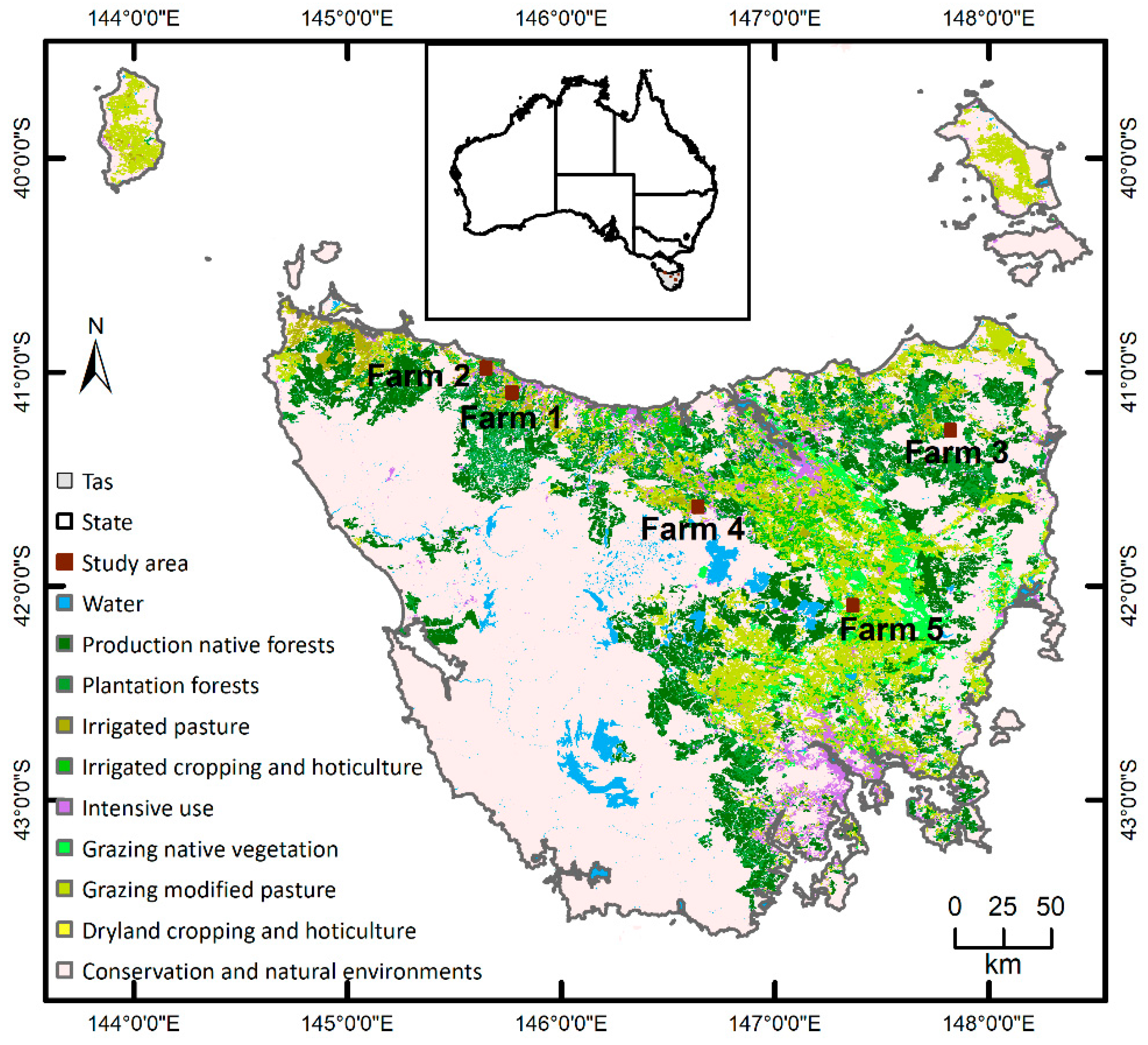
Dairy is Tasmania’s biggest agricultural industry [43]. There were 412 dairy farms in the state in 2019. Tasmania has a suitable/optimal environment due to its rich water resources, growing irrigation investments and absence of major animal diseases, together with a mild temperate climate, fertile soils, reliable rainfall and plenty of sunshine, making it the ideal location for dairy farming. All of these ensure excellent growing conditions for lush pastures (grass and clover) that support the production of premium quality products, particularly livestock [44,45]. For example, Tasmanian milk production has increased by around 38% over the past 10 years, almost double to 1.5 billion litres per year to meet the increasing national and international demands. The study was conducted in five selected dairy farms in the northern part of Tasmania, Australia (Figure 1). The total area of the five farms was 1333 ha. Tasmania has a cool temperate climate with four distinct seasons. The mean annual rainfall is highly differentiated across space and over time. Dairy stocking rates are directly linked to the availability of water. Rainfall increases from around 506 mm in the centre of the region to 2690 mm in the north-western regions. The average maximum temperature in summer (December to February) is 21 °C. The average maximum and minimum temperature (Tmax and Tmin) in winter (June to August) are 12 °C and 4 °C, respectively. Dairy farming in Tasmania is primarily based on the use of perennial pasture species as the major source of feed [46]. Major dairy regions are well suited to perennial ryegrass and white clover with good quality and even feed-supply all year round. The selected combination of five representative dairy farms in this study was motivated by the need to mimic the diversity of the management practice of the dairy industry in Tasmania [44].
2.2. Data Sources
The data used in this study were collected from satellite remote sensing, field observations and interpolated climate raster grids. All the data sources are summarised in Table 1 and described in the following subsections.
2.2.1. Field Biomass Data
Field campaigns across two years were carried out to collect field biomass data in the five selected dairy farms (Figure 2) using traditional agronomic sampling methods from 2017 to 2018 (Table 2). For the sample collection, farm 1 used a C-Dax Pasture Meter (C-Dax Ltd.; http://www.c-dax.co.nz/ (accessed on 8 February 2021)) and the other four farms used a rising plate meter (RPM; [47]). The basic principle was to move around the farm with an instrument that measured pasture height, which was subsequently converted into kilograms of dry matter per hectare (kg DM/ha) using the equation below:
where y is the biomass, x is the height and m (multiplier) and c (constant) are the two manufacturer-supplied calibration factors that can also be further calibrated by users.
y = mx + c,
Pasture biomass from 334 paddocks in these farms was systematically monitored once a week, where the details are provided in Table 2.
2.2.2. Remotely Sensed Data
Time-series S2 MSI surface reflectance data were extracted from the Digital Earth Australia (DEA) database (http://www.ga.gov.au/dea (accessed on 8 February 2021)) for the five farms from 2015 to 2019 (Figure 2). The DEA applies nadir-corrected BRDF adjusted reflectance (NBAR), where BRDF stands for the bidirectional reflectance distribution function. This approach involves atmospheric corrections to compute the bottom-of-atmosphere radiance and bi-directional reflectance modelling to remove the effects of topography and angular variations in the reflectance following Li et al. [48,49]. An additional terrain illumination reflectance correction is performed, and as such, is considered to be the actual surface reflectance, as it considers the surface topography. A full description of the data product and processing can be found in https://cmi.ga.gov.au/data-products/dea/190/surface-reflectance-nbart-1-sentinel-2-msi#basics (accessed on 21 August 2020).
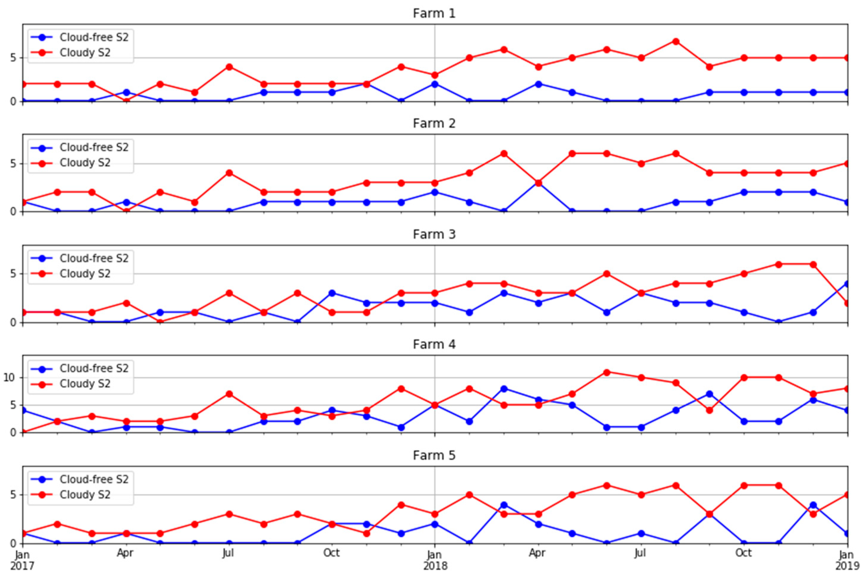
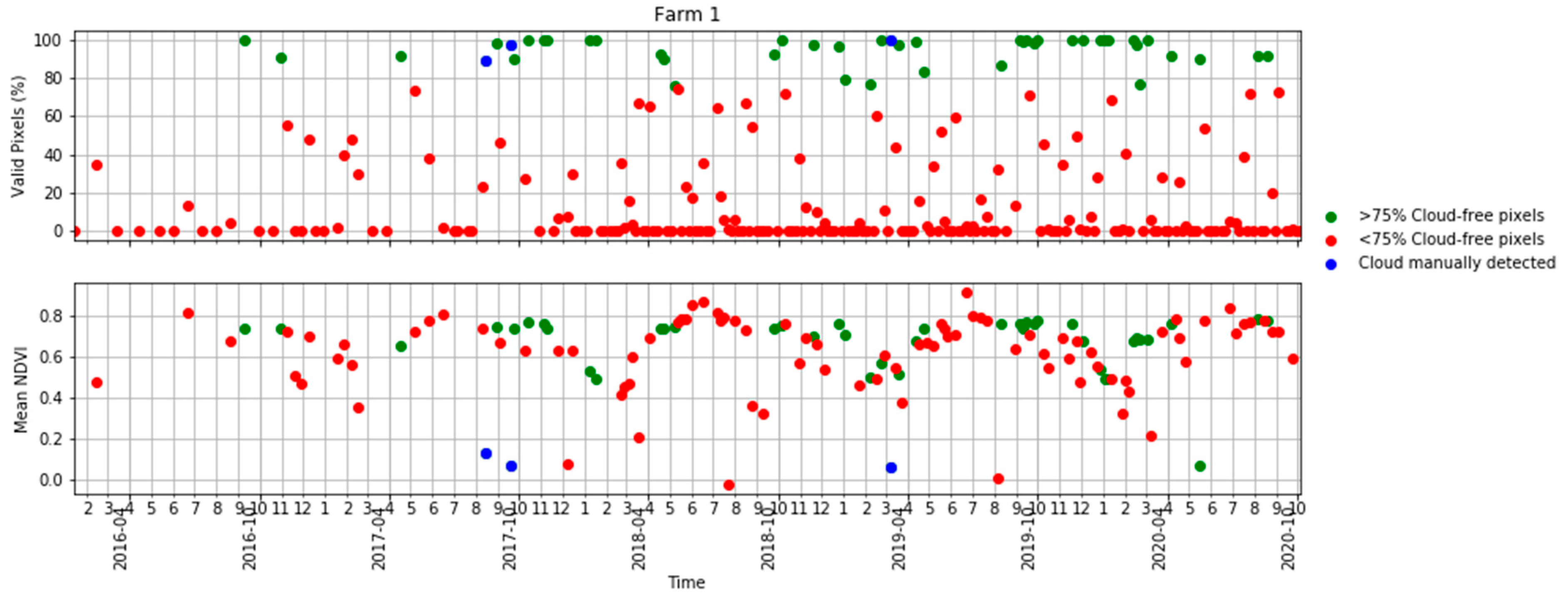
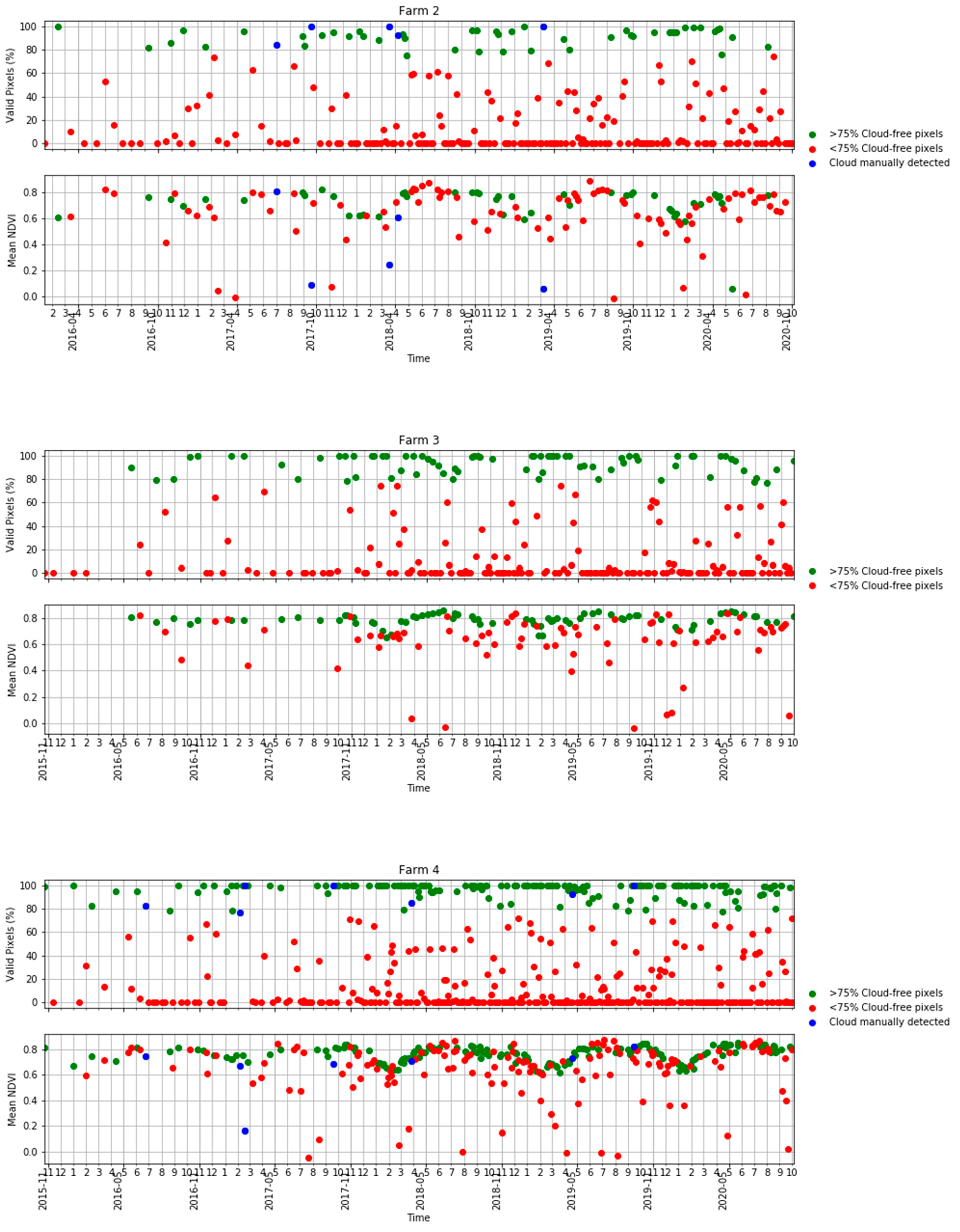
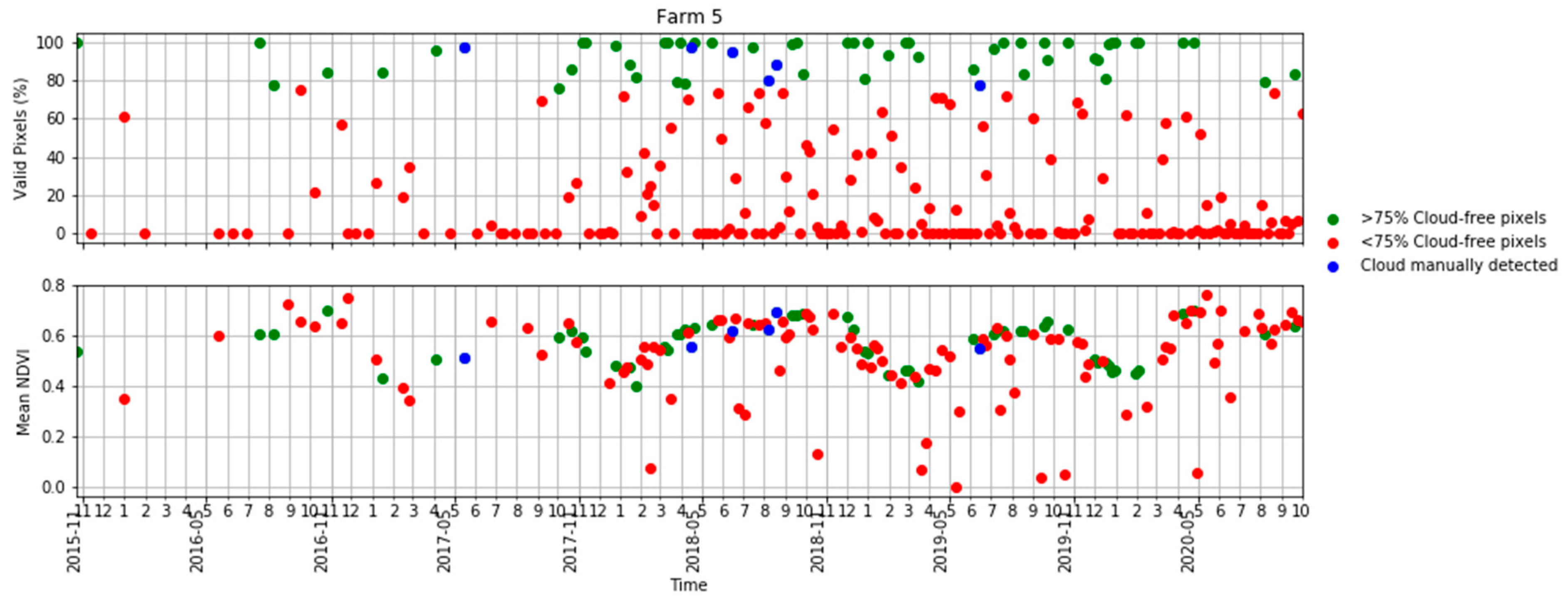
Ten S2 bands, including eight bands in the visible–near infrared and two bands in the shortwave infrared, plus the NDVI derived from bands 7 and 4 were used in this study. The four bands available at a 10 m resolution were aggregated to a 20 m resolution using the nearest-neighbour resampling method. We obtained all available images for each farm. A cloud detection algorithm [50] was applied to the images and those with more than 75% of the pixels affected by clouds or cloud shadows were removed. However, even for those images with more than 75% of pixels being valid, some cloud or cloud shadow images affecting the study areas had to be manually removed using visual interpretation in a quality assurance process. Figure 3 shows a summary of the number of cloud-free and cloud-affected S2 images per farm. Note that farm 4 lay in the overlap of two S2 orbits and, therefore, was covered by twice as many passes as the other four farms. A more comprehensive analysis of the availability of cloud-free imagery in Tasmania and the implications for pasture biomass estimation in dairy production is given in the Appendix A (Figure A1 and Figure A2).
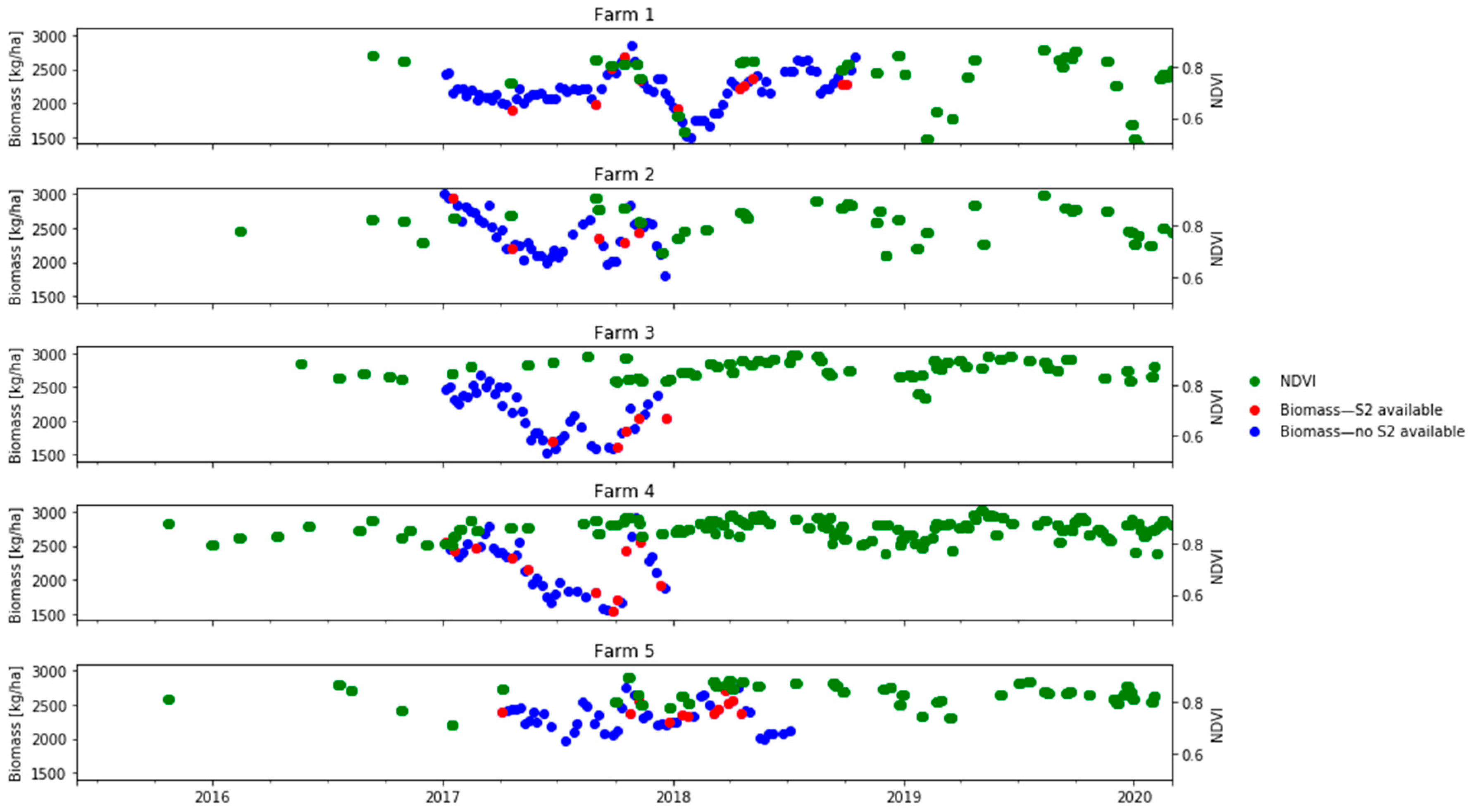
The Sentinel-2 reflectance data was paired with the biomass estimation in each paddock if the satellite overpass was on the same day as the weekly biomass measurement or within a difference of two days (before or after). The median value for each band of all pixels in the paddock was used. Considering the rapid changes in biomass due to intensive grazing in dairy production systems, we avoided pairing biomass and satellite measurements if the two observations were three or more days apart. Given this constraint, Figure 4 shows how many dates of biomass observations (blue dots) did not have a concurrent S2 pair and could not be used for model calibration or evaluation.
2.2.3. Climate Data
To examine climate the variability/variation over time, gridded daily climate data at a 5 km resolution were obtained from the Australian Government Bureau of Meteorology from the Australian Water Availability Project (AWAP; [51]). These included precipitation (P (mm)), maximum temperature (Tmax (°C)), minimum temperature (Tmin (°C)), solar radiation (RAD (W/m2)) and the vapour pressure deficits at 9 am and 3 pm (VPH-09 and VPH-15 (hPa)). We hypothesised that the inclusion of the mean climate conditions antecedent to the biomass measurement could improve the modelled biomass relative to what could be achieved using surface reflectance from S2 only, particularly the amount of rainfall and the mean temperature as main drivers of pasture growth. We used a period of 28 days (4 weeks) before each field sampling date as the additional input variables in our biomass modelling. The detailed rainfall and temperature summary for the five selected dairy farms are presented in Figure 5.
3. Methods
3.1. Correlating the S2 Imagery with In Situ Data
NDVI is the most widely used index used to measure the biophysical properties of vegetation. In this study, it was employed with the expectation of using it as a proxy for biomass for a general understanding of the pasture characteristics across the landscape. Linear least-squares regression was used to initially test the utility of NDVI in estimating the pasture biomass. In situ biomass (kg DM/ha) data from 2017 to 2018 (Table 1), which was measured weekly from paddocks (one record per paddock) in the five farms, were correlated to the NDVI values averaged from pixels within each corresponding paddock in all farms. The results were plotted against each other to establish the relationship between them.
3.2. Developing a Machine Learning Algorithm
We used the TensorFlow software framework (https://www.tensorflow.org (accessed on 8 February 2021)), which is a machine learning system that enables users to experiment with novel optimisations and training algorithms. It supports a variety of applications with a focus on training and inference on neural networks. This open-source platform has a comprehensive set of tools, libraries and community resources that lets researchers push the state-of-the-art in machine learning, and for developers to easily build and deploy machine-learning-powered applications. Running on top of TensorFlow, there is an open-source neural network library written in Python (https://keras.io/ (accessed on 8 February 2021)). It is designed to offer a higher-level, more intuitive set of abstractions that make it easy to develop machine learning models and to enable fast experimentation with neural networks. The merits of being user-friendly, modular and extensible make it a simple, flexible and powerful interface for deep learning.
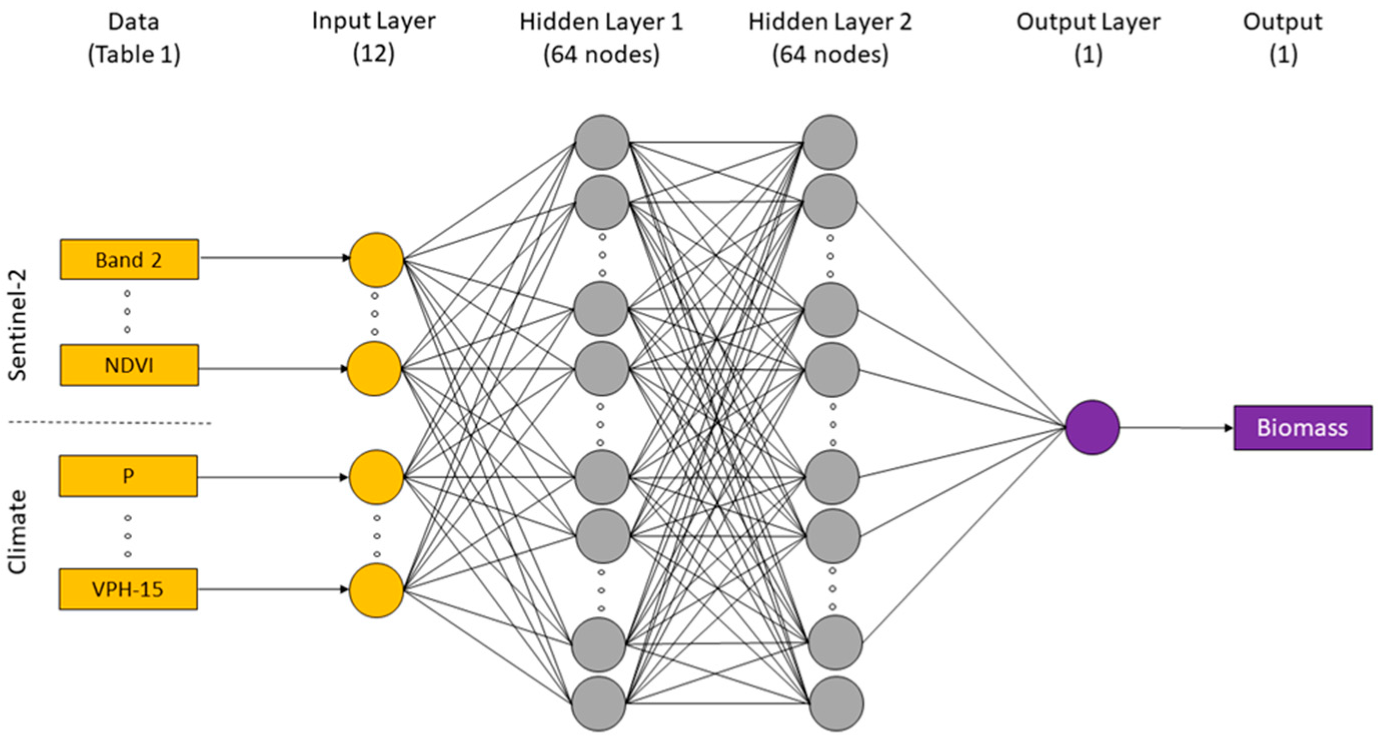
A multilayer perceptron (MLP) neural network model built on the TensorFlow platform was employed in this study. It is one of the simplest forms of an ANN. We chose a model structure with two hidden layers (64 nodes each) and one output (Figure 6). We experimented with adding another hidden layer and varying the number of nodes in each layer, though this provided no substantial improvement in model performance. The activation function chosen was the rectified linear unit and the optimisation algorithm was Adam with a learning rate of 0.001. In each model optimisation, the training was run with a maximum of 3000 epochs but stopped when the model performance (measured in a random subset of 33% of the calibration datasets) did not improve after 50 iterations. The loss function was the root-mean-square error (RMSE), and the metrics evaluated by the model during training and testing were RMSE and the mean absolute error (MAE). The data were normalised before training the model by subtracting the mean and dividing by the standard deviation.
3.3. Modelling Design
The simple ML model in this work served as a potential benchmark with respect to the most complex models requiring parameter optimisation (e.g., [52]). The modelling process was designed as two experiments based on the training of different input datasets:
- (1)
- Experiment 1—The input training data set consisted of all bands of S2 imagery (including NDVI) and the month of the S2 acquisition.
- (2)
- Experiment 2—The same variables as experiment 1 plus the climate variables were used. The climate variables for each farm were the average minimum temperature, maximum temperature, mean temperature, rainfall, radiation, and vapour pressure (Table 1) for the 28 days prior to each ground biomass measurement.
The MLP was used to solve a regression problem in both experiments. The dataset was randomly split as follows: 75% of the data were used for model calibration (training) and the remaining 25% were used for validation (evaluation). Of the data used for calibration, 33% were set aside to test the model performance at each iteration and stop the calibration when the RMSE and MAE stopped improving. We used an arbitrary “patience” parameter of 50 as our choice of the number of training iterations. This early stopping halted the training of the model at about the right time (for 50 iterations) to avoid either overfitting of the training dataset caused by too many iterations or underfitting of the model caused by too few iterations. Finally, a linear least squares regression was employed for evaluating the results of the training and prediction. The performance metrics for the evaluation were the coefficient of determination (R2), MAE and RMSE. A higher R2 and lower MAE and RMSE indicated a better fit with the ground biomass.
3.4. Sensitivity Analysis
To assess the sensitivity of the models to the interfarm variability, we conducted the calibration of experiment 2 (combining S2 and climate variables as inputs) using the leave-one-out approach. We used only the data from four farms for calibration and tested the performance of the model fitted on the paddocks of the fifth farm. We repeated this procedure five times, leaving out data from a different farm each time. This process was aimed at checking whether the differences in the methodology employed to measure the pasture biomass between farm 1 and farms 2 to 5 produced a spurious effect on the estimated biomass.
4. Results and Discussion
4.1. Correlation between In Situ Biomass and the S2 NDVI
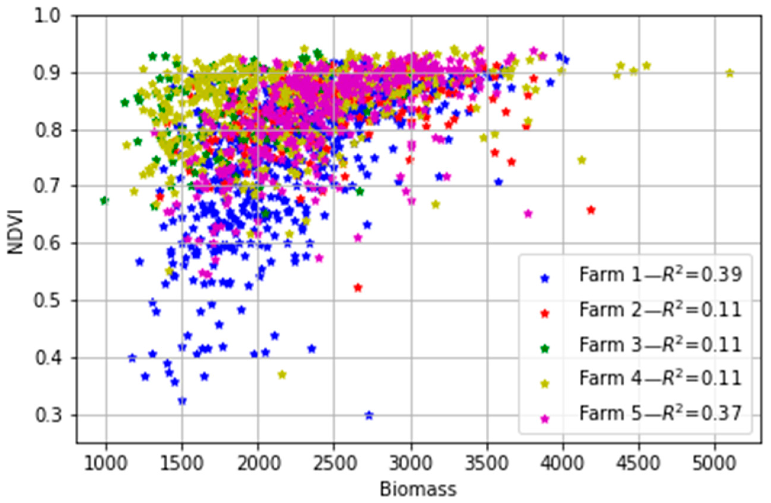
Linear regression analysis between the field biomass measurements and the S2-derived NDVI for all paddocks in the five farms (Figure 7) showed that the NDVI exhibited a generally poor correlation to the pasture biomass (R2 ≤ 0.39). The disagreement between the two datasets means that the commonly used vegetation NDVI cannot be used to directly estimate biomass in the study areas, despite a large body of literature so far showing the utility and robustness of vegetation indices in optimally estimating the aboveground biomass of natural vegetation phenology and crops that follow a steadier transition as compared to dairy pasture (e.g., [14,53,54,55]). It is worth noting that Edirisinghe et al. [56,57] found a similar result, with NDVI and aboveground pasture biomass having a non-linear relationship that depended strongly on the specific farm or pasture type under analysis and changed between dates and became saturated at high biomass levels. The saturation of NDVI at high leaf area index values due to increasing levels of light interception by the canopy is well-known [58]. Furthermore, the soil colour (albedo) and moisture can affect the relationship between NDVI and biomass when the pasture does not cover the soil completely [59,60]. These other factors suggest the alternative of using all the spectral information from the sensor (not just the NDVI) in combination with more advanced methods rather than linear correlations, and the potential of ML as a better approach for estimating the biomass in such an environment. They also highlight the need to consider local vs. aggregated calibrations across both space and time.
4.2. Calibration and Evaluation of the Biomass Estimate from Machine Learning
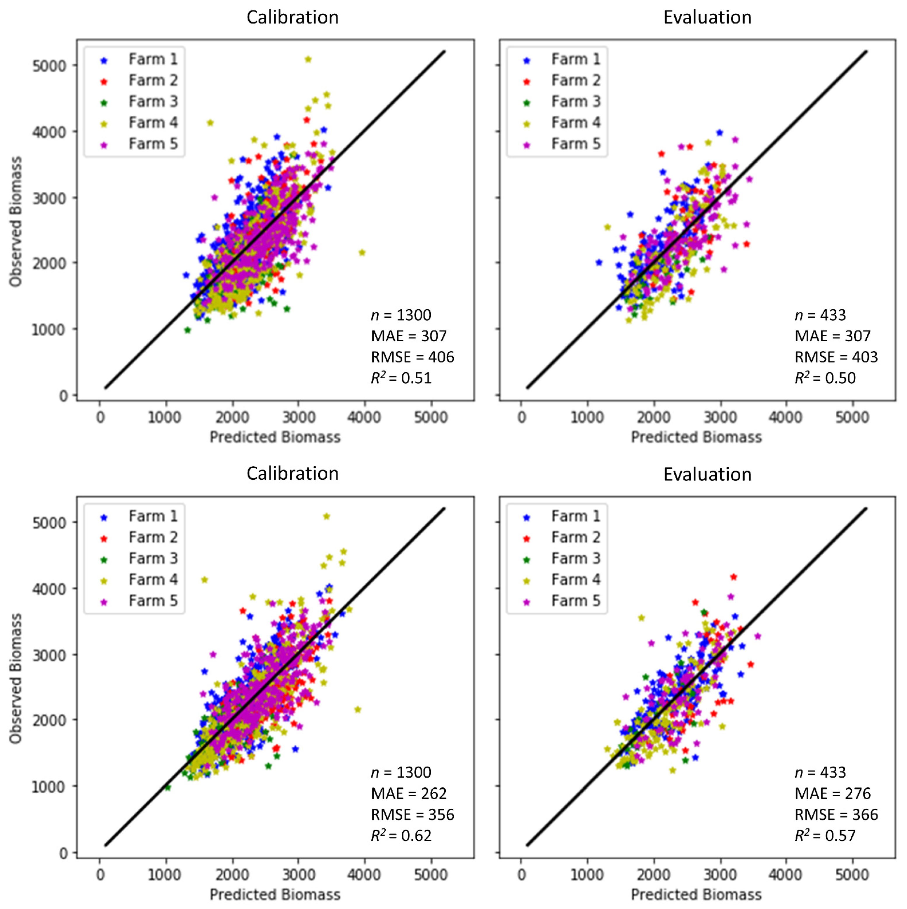
Figure 8 illustrates the accuracies attained in the model calibration and validation (or evaluation) in this study. When the model only included the variables obtained from the S2 reflectance in experiment 1 (Figure 8 top panel), it was able to estimate the aboveground biomass with RMSEs of 406 and 403 kg DM/ha in the calibration and validation subsets, respectively. The MAE was 307 kg DM/ha in both the calibration and validation subsets. As expected, better model performance was obtained when the climate variables reflecting the average conditions in the four weeks before the satellite observation were incorporated as explanatory variables. The RMSE decreased from 406 (403) to 356 (366) kg DM/ha and R2 increased from 0.51 (0.50) to 0.62 (0.57) in the calibration (validation) subsets of experiment 2 (Figure 8 bottom panel). The higher accuracies in both the calibration and validation can be generally quantified with a significant increase of a more than 21% (14%) rise in R2 and a greater than 12% (9%) fall in RMSE in the calibration (validation) subsets in comparison to experiment 1 (Table 3). These results indicate that using S2 data only in experiment 1 provided less accuracy compared to experiment 2, where climate data were added. It also demonstrates that environmental drivers, such as temperature and precipitation, were vital for the grassland biomass. The relatively high level of model prediction accuracy for all farms (R2 = 0.60) achieved in this study means that the optimal model was, therefore, able to explain about 60% of the variability existing in the pasture biomass data. The remaining variance is related to other factors not accounted for in this study, such as the heterogeneity of external environmental and anthropogenic factors, including the grazing rotation, soil types and planting/tilling practices, and field-measurement errors leading to different biomass responses across the farms. The modelling performance metrics obtained in this work are nonetheless comparable to the findings of some of the aforementioned studies. For instance, Shafian et al. [55] and Battude et al. [61] reported similar accuracy, and both Habyarimana et al. [37] and Gao et al. [62] reported lower accuracies. It is worth noting that the reported accuracies of the reference methods (RPM and C-Dax) are also in the order of 437–773 kg DM/ha [63], which indicates that the methods presented here are reaching the potential compared to those reference methods. Therefore, machine learning appears to be a useful approach for remotely sensed biomass estimation when appropriately deployed. The selected ML algorithm outperformed the commonly used NDVI regarding quantifying dairy pasture biomass as a saturated NDVI and the same biomass in different pasture types may end up having the same NDVI. The improved ML performance from an R2 below 0.40 to over 0.50 could be attributed to the ability to automatically identify trends and patterns inherent in a huge amount of data. The optimal models that had the potential to be deployed for estimating pasture biomass across all five farms in the study area were the ones integrating both Sentinel-2 imagery and climate data. The inclusion of climate data led to a general improvement in both the model calibration for model development and validation for result evaluation. This was because environmental drivers, such as temperature and precipitation, play an important part in grassland biomass production. Although the use of the S2 dataset in conjunction with the efficient and robust ML algorithm in this study proved the applicability of ML to the accuracy improvement of pasture biomass prediction, it is well known that biomass yields are largely constrained by water availability, which is driven by edaphic and climatic factors. Incorporating a more thorough understanding of how growing season temperature and precipitation affect aboveground biomass productivity is necessary to advance our understanding of grassland biomass productivity dynamics in the face of climate change. One approach to this may be to couple the outputs of a biophysical model with inputs and parameterisation from satellite imagery. The ML approach used here could then be used to parameterise the biophysical model, therein integrating spatial (satellite imagery) within environmental and physiological frameworks (biophysical models).
4.3. Model Sensitivity to Different Farms
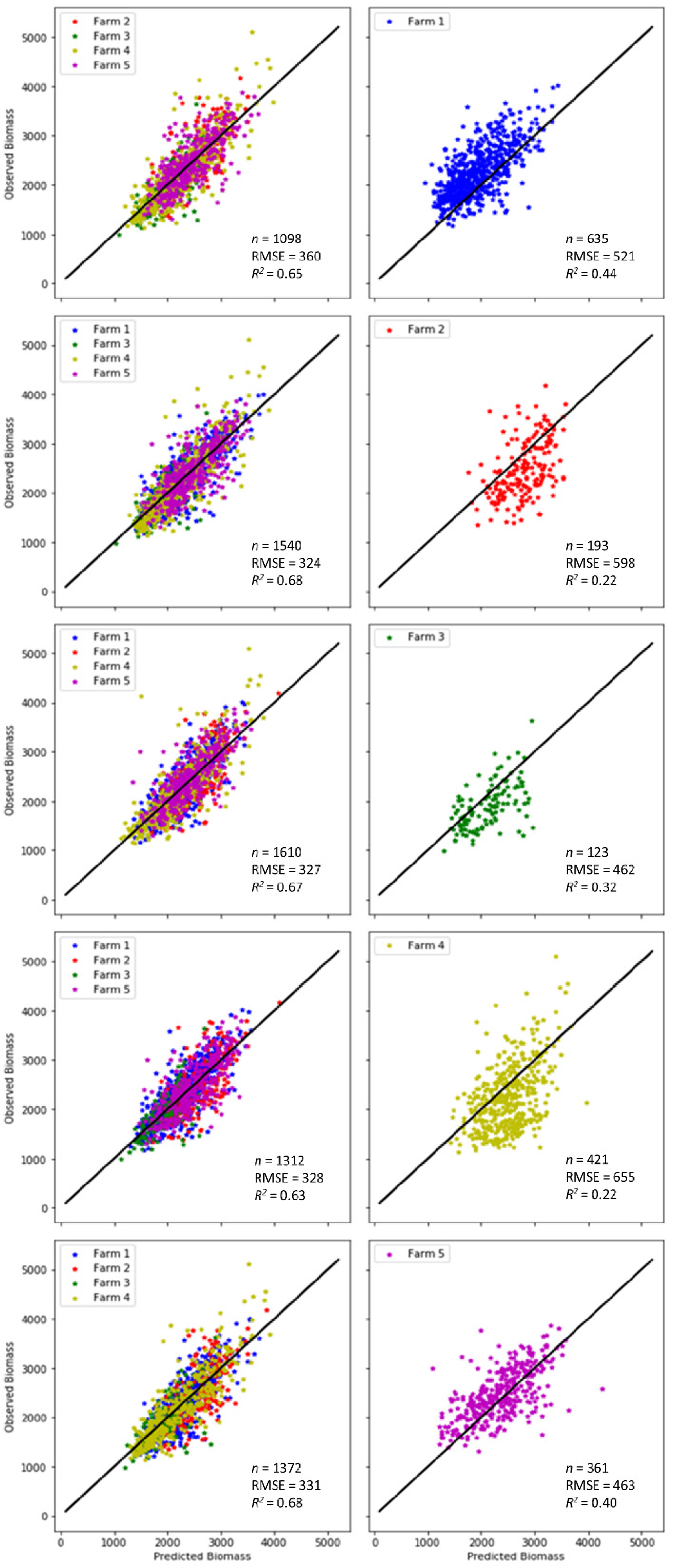
A simple yet powerful way to understand a machine learning model and its outputs is through sensitivity analysis, which can be used to assess what impact each feature/parameter/variable has on the model’s prediction. The sensitivity of the model to each farm was evaluated by removing data from an individual farm from the model calibration, then calibrating the model with the data from the other four farms, and finally applying the model output to the farm that was left out. This was done with the S2 and climate variables, i.e., the same as experiment 2. If an outcome drastically changed, this meant that this farm had a big impact on the prediction resulting from its large bearing on the parameterisation of the algorithm. The results of the sensitivity analysis are plotted in Figure 9 and summarised as the calibration accuracy and validation accuracy in Table 3. In terms of the calibration accuracy, an improvement in both R2 and RMSE for almost all farms can be observed compared to the model calibrated using all farms in experiment 2, except for a minor increase of RMSE for farm 1. In general, all farms contributed equally to the model calibration without a single farm being sensitive to the reduction of training data samples due to its exclusion from the calibration. However, in terms of the evaluation accuracy, all models had a substantial decline in both R2 and RMSE, although farms 1 and 5 outperformed the other three farms, with the smallest drop from 0.57 to 0.40 in R2 for the former, and the smallest rise from 366 to 436 (kg DM/ha) in RMSE for the latter, respectively. The skewed verifications could be attributed to the bias in the field measurements resulting from using the C-Dax in farm 1 and the rising plate meters in the other four farms. Noticeably, farm 4 was the worst with the lowest R2 and the highest RMSE among all farms, and therefore, the most sensitive farm against all others. The poor evaluation accuracy for farms 2 and 4, despite their good calibration accuracy, implies the strong influence of farm-specific factors, which had significant impacts on the biomass prediction. Therefore, the sensitivity analysis employed in this study offers a simple and intuitive technique to help users understand which farms most influence the ML model.
4.4. Cloud Issues in the Time-Series Biomass Estimation
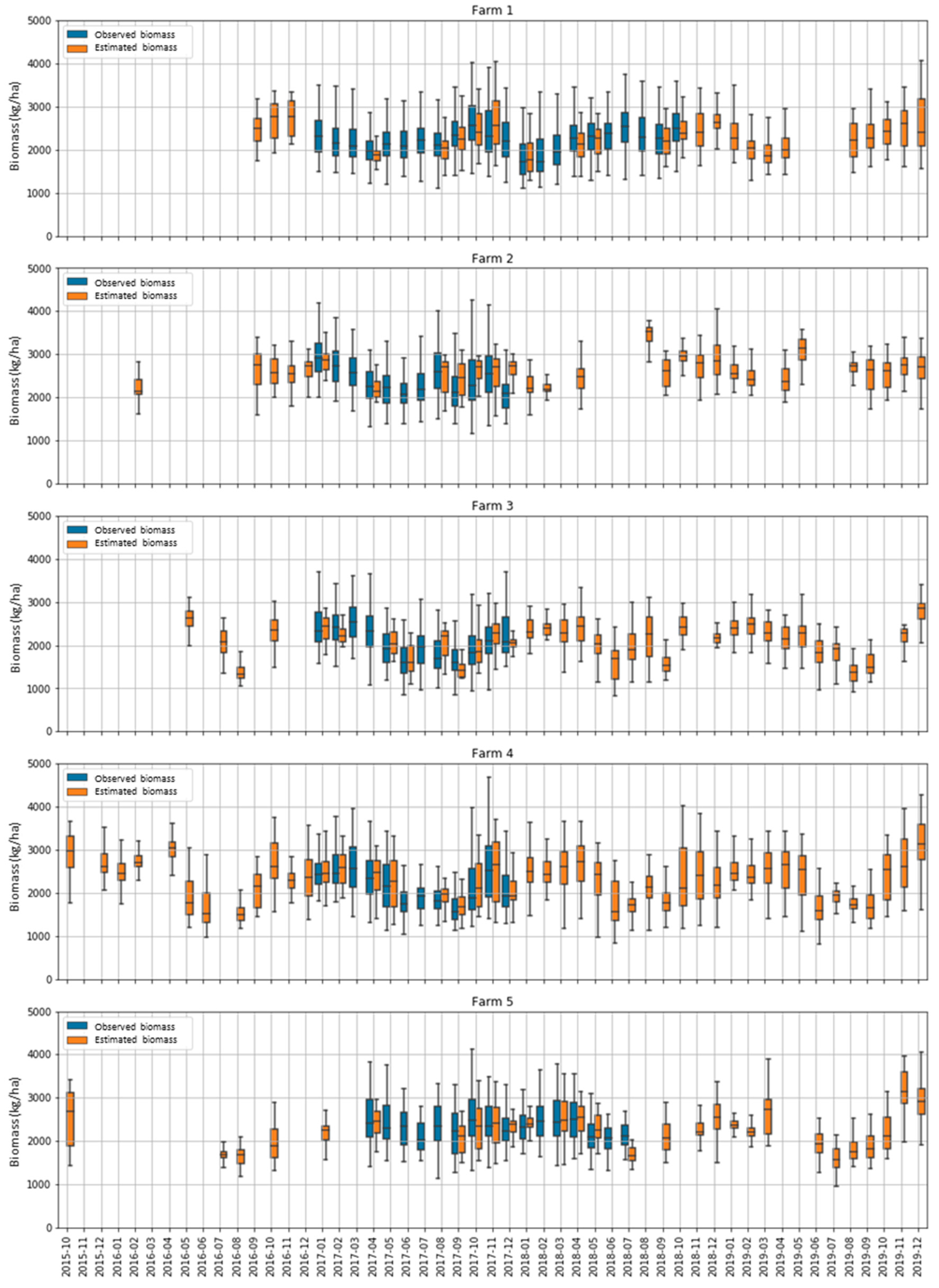
To explore seasonal patterns in the biomass estimations in all farms and paddocks, we repeated the calibration of experiment 2 using all the data available (i.e., not splitting between the calibration and evaluation). The model was then applied to all dates with available cloud-free S2 imagery. All farms showed a seasonal pattern of estimated biomass that increased in the late spring and summer months and decreased during the winter (Figure 10). The range of estimated biomass values (i.e., amplitude of the box plots) closely followed the range of the observed values. Unfortunately, it can be observed that although the freely available S2 images have demonstrated potential benefits in biomass estimation over traditional field measurement methods in a cost-effective and relatively quick manner, their applications for dairy pasture could be hampered by the cloud issues in Tasmania during the study period. The temporal resolution of the S2 time series was affected by frequent cloud cover, which significantly reduced the number of good quality images in this study.
Figure 9 (and Figure 2) also highlight that, even with the two Sentinel-2 satellites (A and B) sampling each point on Earth every 5 days, there were often gaps of 1, 2 or even 3 consecutive months without good S2 observations due to highly frequent cloud cover in many parts of Tasmania, particularly the northwestern areas. This can be a problem for the dairy industry, which needs very frequent and near-real-time biomass estimations for decision-making regarding grazing management. Hence, our future work will focus on the fusion of multi-sensor data at a medium-to-high spatio-temporal resolution to address this issue. Furthermore, optical sensor imagery is generally suitable for extracting information about simple and homogeneous grasslands. In combination with the synthetic aperture radar (SAR), the simultaneous use of spectral information and image texture parameters could enhance the value for the biomass assessment of heterogeneous complex biophysical environments [64,65].
5. Conclusions
This study examined the potential for estimating pasture biomass on dairy farms from Sentinel-2 imagery using machine learning. Around 60% of the variability in biomass was explained through integrating time-series S2 images, in situ observations and climate data in a simple machine learning algorithm. The best model was able to estimate biomass with an RMSE of ≈356 kg DM/ha (MAE of 262 kg DM/ha). This result was within the variability of the pasture biomass measured in the field, and therefore represents relatively high accuracy and a good possibility for integration in a framework used to predict pasture biomass at a regional scale. Although the approach remains to be tested at larger scales and on diverse pasture botanical compositions and management practices, this study demonstrated the potential of Sentinel-2 data and climate variables for capturing spatio-temporal changes in pasture biomass at the paddock level by providing improved estimation in dairy agricultural landscapes using machine learning. The approach offers an opportunity to develop operational pasture monitoring systems that are less dependent on site-specific calibrations.
To the best of our knowledge, this work is the first attempt to integrate Sentinel-2 and machine learning for estimating biomass in dairy pastures among very few similar applications in the world. The outcome from this study is important and can serve several purposes, including farmers being able to improve their business operations through better biomass management. Policymakers will also benefit from the findings in this investigation by providing them with early within-season potential biomass availability, which is critical for wider pasture–production planning and avoiding climate/water-related crises.
Author Contributions
Field data collection and processing, M.T.H., Y.S., D.H. and Y.C.; modelling, J.G., Y.C. and Y.S.; manuscript writing, Y.C. and J.G.; review and editing, Y.S., M.T.H. and D.H. All authors have read and agreed to the published version of the manuscript.
Funding
This research received no external funding.
Acknowledgments
We would like to acknowledge and thank the staff at the Tasmanian Institute of Agriculture for the collection and processing of many samples over many years, and the participating Tasmanian dairy farmers since without their collaboration, this project could not have been possible. We are grateful to Jorge Peña Arancibia and Phillip Ford (both from Commonwealth Scientific and Industrial Research Organisation (CSIRO) Land and Water, Australia) for kindly reviewing the manuscript.
Conflicts of Interest
The authors declare no conflict of interest.
Appendix A. Cloud Coverage Analysis of the Sentinel-2 Imagery
Figure A1.
Time series of the percentage of valid pixels in each S2 scene (top) and mean NDVI (bottom) in Table 2 in terms of scenes with >75% valid pixels, <75% valid pixels and S2 scenes visually identified as clouds.
Figure A1.
Time series of the percentage of valid pixels in each S2 scene (top) and mean NDVI (bottom) in Table 2 in terms of scenes with >75% valid pixels, <75% valid pixels and S2 scenes visually identified as clouds.


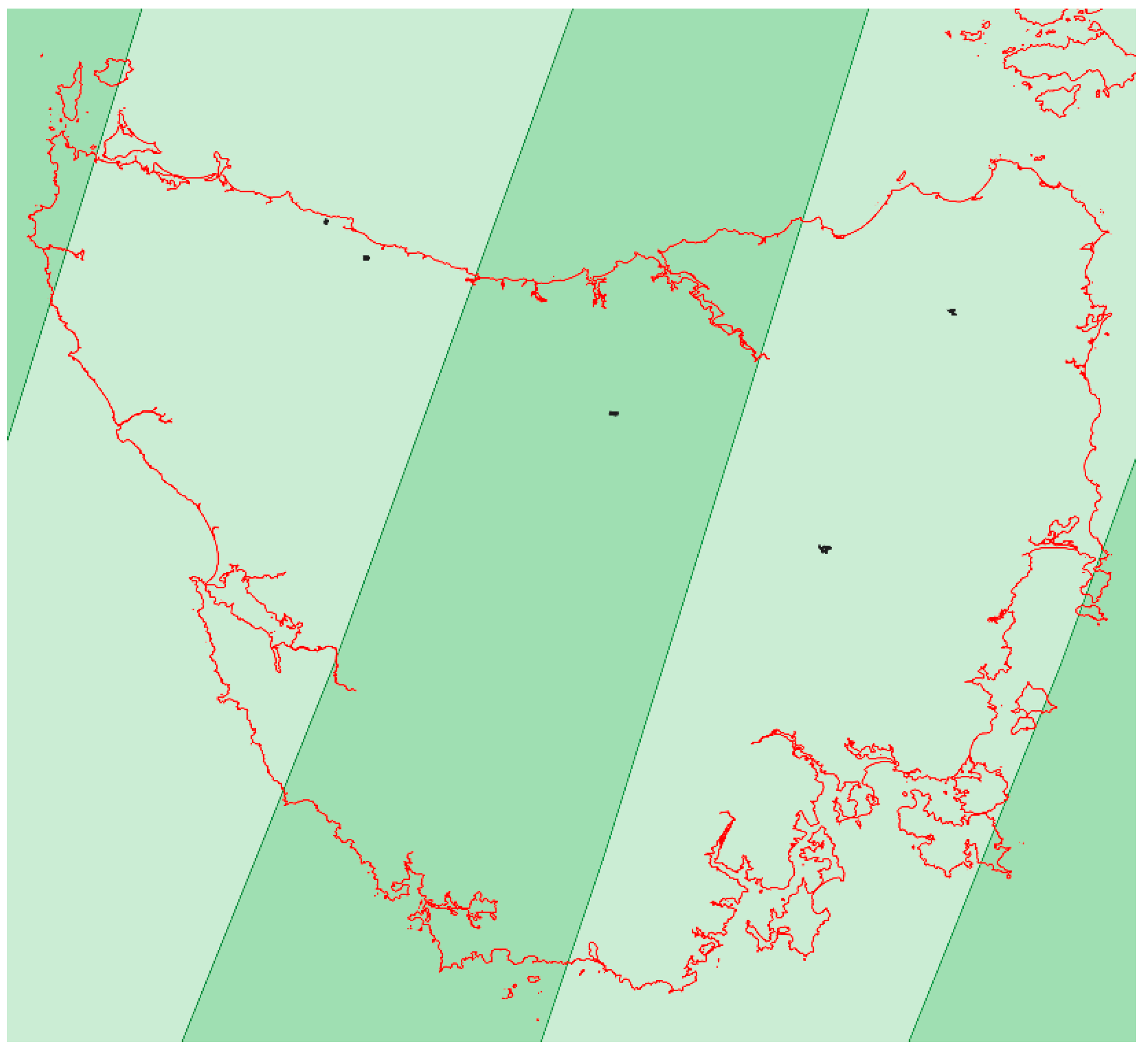
Figure A2.
Map of Tasmania showing the areas with a single Sentinel-2 orbit (light green) and the areas where two Sentinel-2 orbits overlapped (dark green). The five farms of this study are shown.
Figure A2.
Map of Tasmania showing the areas with a single Sentinel-2 orbit (light green) and the areas where two Sentinel-2 orbits overlapped (dark green). The five farms of this study are shown.

References
- Chang-Fung-Martel, J.; Harrison, M.T.; Rawnsley, R.; Smith, A.P.; Meinke, H. The impact of extreme climatic events on pasture-based dairy systems: A review. Crop Pasture Sci. 2017, 68, 1158–1169. [Google Scholar] [CrossRef]
- Hovenden, M.; Newton, P.; Wills, K. Seasonal not annual rainfall determines grassland biomass response to carbon dioxide. Nature 2014, 511, 583–586. [Google Scholar] [CrossRef] [PubMed]
- Bell, L.W.; Harrison, M.T.; Kirkegaard, J.A. Dual-purpose cropping—Capitalising on potential grain crop grazing to enhance mixed-farming profitability. Crop Pasture Sci. 2015, 66, i–iv. [Google Scholar] [CrossRef] [Green Version]
- Harrison, M.T.; Evans, J.R.; Dove, H.; Moore, A.D. Recovery dynamics of rainfed winter wheat after livestock grazing 2. Light interception, radiation-use efficiency and dry-matter partitioning. Crop Pasture Sci. 2011, 62, 960–971. [Google Scholar] [CrossRef]
- Hakl, J.; Hrevušová, Z.; Hejcman, M.; Fuksa, P. The use of a rising plate meter to evaluate lucerne (Medicago sativa L.) height as an important agronomic trait enabling yield estimation. Grass Forage Sci. 2012, 67, 589–596. [Google Scholar] [CrossRef]
- Psomas, A.; Kneubühler, M.; Huber, S.; Itten, K.; Zimmermann, N.E. Hyperspectral remote sensing for estimating aboveground biomass and for exploring species richness patterns of grassland habitats. Int. J. Remote Sens. 2011, 32, 9007–9031. [Google Scholar] [CrossRef]
- King, W.M.; Rennie, G.M.; Dalley, D.E.; Dynes, R.A.; Upsdell, M.P. Pasture Mass Estimation by the C-Dax Pasture Meter: Regional Calibrations for New Zealand. In Proceedings of the 4th Australasian Dairy Science Symposium, Lincoln, New Zealand, 31 August–2 September 2010. [Google Scholar]
- Chen, Y.; Gillieson, D. Evaluations of Landsat TM vegetation indices for estimating vegetation cover on semi-arid rangelands—A case study from Australia. Can. J. Remote Sens. 2009, 35, 435–446. [Google Scholar] [CrossRef]
- Pembleton, K.G.; Cullen, B.R.; Rawnsley, R.P.; Harrison, M.T.; Ramilan, T. Modelling the resilience of forage crop production to future climate change in the dairy regions of Southeastern Australia using APSIM. J. Agric. Sci. 2016, 154, 1131–1152. [Google Scholar] [CrossRef]
- Harrison, M.T.; Jackson, T.; Cullen, B.R.; Rawnsley, R.P.; Ho, C.; Cummins, L.; Eckard, R.J. Increasing ewe genetic fecundity improves whole-farm production and reduces greenhouse gas emissions intensities: 1. Sheep production and emissions intensities. Agric. Syst. 2014, 131, 23–33. [Google Scholar] [CrossRef]
- Harrison, M.T.; Cullen, B.R.; Armstrong, D. Management options for dairy farms under climate change: Effects of intensification, adaptation and simplification on pastures, milk production and profitability. Agric. Syst. 2017, 155, 19–32. [Google Scholar] [CrossRef]
- Kumar, L.; Sinha, P.; Taylor, S.; Alqurashi, A.F. Review of the use of remote sensing for biomass estimation to support renewable energy generation. J. Appl. Remote Sens. 2015, 9, 097696. [Google Scholar] [CrossRef]
- Chen, Y.; Guerschman, J.; Cheng, Z. Remote sensing for vegetation monitoring in Carbon Capture Storage regions: A review. Appl. Energy 2019, 240, 312–326. [Google Scholar] [CrossRef]
- Sibanda, M.; Mutanga, O.; Rouget, M. Examining the potential of Sentinel-2 MSI spectral resolution in quantifying above ground biomass across different fertilizer treatments. ISPRS J. Photogramm. Remote Sens. 2015, 110, 55–65. [Google Scholar] [CrossRef]
- Filho, M.G.; Kuplich, T.M.; De Quadros, F.L.F. Estimating natural grassland biomass by vegetation indices using Sentinel 2 remote sensing data. Int. J. Remote Sens. 2020, 41, 2861–2876. [Google Scholar] [CrossRef]
- Drusch, M.; Del Bello, U.; Carlier, S.; Colin, O.; Fernandez, V.; Gascon, F.; Hoersch, B.; Isola, C.; Laberinti, P.; Martimort, P.; et al. Sentinel-2: ESA’s optical high-resolution mission for GMES operational services. Remote Sens. Environ. 2012, 120, 25–36. [Google Scholar] [CrossRef]
- Wylie, B.K.; Harrington, J.A.; Prince, S.D.; Denda, I. Satellite and ground-based pasture production assessment in Niger: 1986–1988. Int. J. Remote Sens. 1991, 12, 1281–1300. [Google Scholar] [CrossRef]
- Anderson, G.; Hanson, J.; Haas, R. Evaluating Landsat Thematic Mapper derived vegetation indices for estimating above-ground biomass on semiarid rangelands. Remote Sens. Environ. 1993, 45, 165–175. [Google Scholar] [CrossRef]
- Zha, Y.; Gao, J.; Ni, S.; Liu, Y.; Jiang, J.; Wei, Y. A spectral reflectance-based approach to quantification of grassland cover from Landsat TM imagery. Remote Sens. Environ. 2003, 87, 371–375. [Google Scholar] [CrossRef]
- Boschetti, M.; Bocchi, S.; Brivio, P.A. Assessment of pasture production in the Italian Alps using spectrometric and remote sensing information. Agric. Ecosyst. Environ. 2007, 118, 267–272. [Google Scholar] [CrossRef]
- Dusseux, P.; Hubert-Moy, L.; Corpetti, T.; Vertès, F. Evaluation of SPOT imagery for the estimation of grassland biomass. Int. J. Appl. Earth Obs. Geoinf. 2015, 38, 72–77. [Google Scholar] [CrossRef]
- Wylie, B.; Meyer, D.; Tieszen, L.; Mannel, S. Satellite mapping of surface biophysical parameters at the biome scale over the North American grasslands: A case study. Remote Sens. Environ. 2002, 79, 266–278. [Google Scholar] [CrossRef]
- Vescovo, L.; Gianelle, D. Using the MIR bands in vegetation indices for the estimation of grassland biophysical parameters from satellite remote sensing in the Alps region of Trentino (Italy). Adv. Space Res. 2008, 41, 1764–1772. [Google Scholar] [CrossRef]
- Punalekar, S.M.; Verhoef, A.; Quaife, T.L.; Humphries, D.; Bermingham, L.; Reynolds, C.K. Application of Sentinel-2A data for pasture biomass monitoring using a physically based radiative transfer model. Remote Sens. Environ. 2018, 218, 207–220. [Google Scholar] [CrossRef]
- Gargiulo, J.; Clark, C.; Lyons, N.; Veyrac, G.; Beale, P.; Garcia, S. Spatial and temporal pasture biomass estimation integrating Electronic Plate Meter, Planet CubeSats and Sentinel-2 Satellite Data. Remote Sens. 2020, 12, 3222. [Google Scholar] [CrossRef]
- Ali, I.; Greifeneder, F.; Stamenkovic, J.; Neumann, M.; Notarnicola, C. Review of machine learning approaches for biomass and soil moisture retrievals from remote sensing data. Remote Sens. 2015, 7, 16398–16421. [Google Scholar] [CrossRef] [Green Version]
- Cutler, M.E.J.; Boyd, D.S.; Foody, G.M.; Vetrivel, A. Estimating tropical forest biomass with a combination of SAR image texture and Landsat TM data, An assessment of predictions between regions. ISPRS J. Photogramm. Remote Sens. 2012, 70, 66–77. [Google Scholar] [CrossRef] [Green Version]
- Dang, A.T.N.; Nandy, S.; Srinet, R.; Luong, N.V.; Ghosh, S.; Kumar, A.S. Forest aboveground biomass estimation using machine learning regression algorithm in Yok Don National Park, Vietnam. Ecol. Inform. 2019, 50, 24–32. [Google Scholar] [CrossRef]
- Ghosh, S.M.; Behera, M.D. Aboveground biomass estimation using multi-sensor data synergy and machine learning algorithms in a dense tropical forest. Appl. Geogr. 2018, 96, 29–40. [Google Scholar] [CrossRef]
- Zhang, L.; Shao, Z.; Liu, J.; Cheng, Q. Deep learning based retrieval of forest aboveground biomass from combined LiDAR and Landsat 8 data. Remote Sens. 2019, 11, 1459. [Google Scholar] [CrossRef] [Green Version]
- Shao, Z.; Shang, L. Estimating forest aboveground biomass by combining optical and SAR Data: A case study in Genhe, Inner Mongolia, China. Sensors 2016, 16, 834. [Google Scholar] [CrossRef] [Green Version]
- Zhang, L.; Shao, Z.; Diao, C. Synergistic retrieval model of forest biomass using the integration of optical and microwave remote sensing. J. Appl. Remote Sens. 2015, 9, 096069. [Google Scholar] [CrossRef]
- Zhang, Y.; Shao, Z. Assessing of urban vegetation biomass in combination with LiDAR and high-resolution remote sensing images. Int. J. Remote Sens. 2021, 42, 964–985. [Google Scholar] [CrossRef]
- Ji, B.; Sun, Y.; Yang, S.; Wan, J. Artificial neural networks for rice yield prediction in mountainous regions. J. Agric. Sci. 2007, 145, 249–261. [Google Scholar] [CrossRef]
- Panda, S.S.; Ames, D.P.; Panigrahi, S. Application of vegetation indices for agricultural crop yield prediction using neural network techniques. Remote Sens. 2010, 2, 673–696. [Google Scholar] [CrossRef] [Green Version]
- Uno, Y.; Prasher, S.O.; Lacroix, R.; Goel, P.K.; Karimi, Y.; Viau, A.; Patel, R.M. Artificial neural networks to predict corn yield from Compact Airborne Spectrographic Imager data. Comput. Electron. Agric. 2005, 47, 149–161. [Google Scholar] [CrossRef]
- Habyarimana, E.; Piccard, I.; Catellani, M.; Franceschi, P.D.; Dall’Agata, M. Towards predictive modelling of sorghum biomass yields using fraction of absorbed photosynthetically active radiation derived from Sentinel-2 satellite imagery and supervised machine learning techniques. Agronomy 2019, 9, 203. [Google Scholar] [CrossRef] [Green Version]
- Jin, X.; Li, Z.; Feng, H.; Ren, Z.; Li, S. Deep neural network algorithm for estimating maize biomass based on simulated Sentinel 2A vegetation indices and leaf area index. Crop J. 2020, 8, 87–97. [Google Scholar] [CrossRef]
- Xie, Y.; Sha, Z.; Yu, M.; Bai, Y.; Zhang, L. A comparison of two models with Landsat data for estimating above ground grassland biomass in Inner Mongolia, China. Ecol. Model. 2009, 220, 1810–1818. [Google Scholar] [CrossRef]
- Ali, I.; Cawkwell, F.; Green, S.; Dwyer, N. Application of statistical and machine learning models for grassland yield estimation based on a hypertemporal satellite remote sensing time series. In Proceedings of the 2014 IEEE International Geoscience and Remote Sensing Symposium (IGARSS 2014), Quebec City, QC, Canada, 13–18 July 2014; pp. 5060–5063. [Google Scholar]
- Ali, I.; Cawkwell, F.; Dwyer, E.; Green, S. Modeling managed grassland biomass estimation by using multitemporal remote sensing data—A machine learning approach. IEEE J. Sel. Top. Appl. Earth Obs. Remote Sens. 2017, 10, 3254–3264. [Google Scholar] [CrossRef]
- Griffiths, P.; Nendel, C.; Pickert, J.; Hostert, P. Towards national-scale characterization of grassland use intensity from integrated Sentinel-2 and Landsat time series. Remote Sens. Environ. 2020, 238, 111124. [Google Scholar] [CrossRef]
- Dairy Tas. The Dairy Industry in Tasmania; Tasmania Government: Hobart, Australia, 2019.
- Phelan, D.C.; Harrison, M.T.; Kemmerer, E.P.; Parsons, D. Management opportunities for boosting productivity of cool-temperate dairy farms under climate change. Agric. Syst. 2015, 138, 46–54. [Google Scholar] [CrossRef]
- Christie, K.M.; Smith, A.P.; Rawnsley, R.P.; Harrison, M.T.; Eckard, R.J. Simulated seasonal responses of grazed dairy pastures to nitrogen fertilizer in SE Australia: Pasture production. Agric. Syst. 2018, 166, 36–47. [Google Scholar] [CrossRef]
- Harrison, M.T.; Christie, K.M.; Rawnsley, R.P.; Eckard, R.J. Modelling pasture management and livestock genotype interventions to improve whole-farm productivity and reduce greenhouse gas emissions intensities. Anim. Prod. Sci. 2014, 54, 2018–2028. [Google Scholar] [CrossRef]
- Rayburn, E.B.; Rayburn, S.B. A standardized plate meter for estimating pasture mass in on-farm research trials. Agron. J. 1998, 90, 238–241. [Google Scholar] [CrossRef]
- Li, F.; Jupp, D.L.B.; Reddy, S.; Lymburner, L.; Mueller, N.; Tan, P.; Islam, A. An evaluation of the use of atmospheric and BRDF correction to standardize Landsat data. IEEE J. Sel. Top. Appl. Earth Obs. Remote Sens. 2010, 3, 257–270. [Google Scholar] [CrossRef]
- Li, F.; Jupp, D.L.B.; Thankappan, M.; Lymburner, L.; Mueller, N.; Lewis, A.; Held, A. A physics-based atmospheric and BRDF correction for Landsat data over mountainous terrain. Remote Sens. Environ. 2012, 124, 756–770. [Google Scholar] [CrossRef]
- Foga, S.; Scaramuzza, P.L.; Guo, S.; Zhu, Z.; Dilley, R.D.; Beckmann, T.; Schmidt, G.L.; Dwyer, J.L.; Joseph Hughes, M.; Laue, B. Cloud detection algorithm comparison and validation for operational Landsat data products. Remote Sens. Environ. 2017, 194, 379–390. [Google Scholar] [CrossRef] [Green Version]
- Jones, D.A.; Wang, W.; Fawcett, R. High-quality spatial climate datasets for Australia. Aust. Meteorol. Oceanogr. J. 2009, 58, 233–248. [Google Scholar] [CrossRef]
- Harrison, M.T.; Roggero, P.P.; Zavattaro, L. Simple, efficient and robust techniques for automatic multi-objective function parameterisation: Case studies of local and global optimisation using APSIM. Environ. Model. Softw. 2019, 117, 109–133. [Google Scholar] [CrossRef]
- Clevers, J.G.; Gitelson, A.A. Remote estimation of crop and grass chlorophyll and nitrogen content using red-edge bands on Sentinel-2 and-3. Int. J. Appl. Earth Obs. Geoinf. 2013, 23, 344–351. [Google Scholar] [CrossRef]
- Helman, D.; Mussery, A.; Lensky, I.M.; Leu, S. Detecting changes in biomass productivity in a different land management regime in drylands using satellite-derived vegetation index. Soil Use Manag. 2014, 30, 32–39. [Google Scholar] [CrossRef]
- Shafian, S.; Rajan, N.; Schnell, R.; Bagavathiannan, M.; Valasek, J.; Shi, Y.; Olsenholler, J. Unmanned aerial systems-based remote sensing for monitoring sorghum growth and development. PLoS ONE 2018, 13, e0196605. [Google Scholar] [CrossRef] [PubMed] [Green Version]
- Edirisinghe, A.; Hill, M.J.; Donald, G.E.; Hyder, M. Quantitative mapping of pasture biomass using satellite imagery. Int. J. Remote Sens. 2011, 32, 2699–2724. [Google Scholar] [CrossRef]
- Edirisinghe, A.; Clark, D.; Waugh, D. Spatio-temporal modelling of biomass of intensively grazed perennial dairy pastures using multispectral remote sensing. Int. J. Appl. Earth Obs. Geoinf. 2012, 16, 5–16. [Google Scholar] [CrossRef]
- Garroutte, E.L.; Hansen, A.J.; Lawrence, R.L. Using NDVI and EVI to map spatiotemporal variation in the biomass and quality of forage for migratory elk in the Greater Yellowstone Ecosystem. Remote Sens. 2016, 8, 404. [Google Scholar] [CrossRef] [Green Version]
- Huete, A.; Didan, K.; Miura, T.; Rodriguez, E.P.; Gao, X.; Ferreira, L.G. Overview of the radiometric and biophysical performance of the MODIS vegetation indices. Remote Sens. Environ. 2002, 83, 195–213. [Google Scholar] [CrossRef]
- Matsushita, B.; Yang, W.; Chen, J.; Onda, Y.; Qiu, G. Sensitivity of the Enhanced Vegetation Index (EVI) and Normalized Difference Vegetation Index (NDVI) to topographic effects: A case study in high-density cypress forest. Sensors 2007, 7, 2636–2651. [Google Scholar] [CrossRef] [PubMed] [Green Version]
- Battude, M.; Al Bitar, A.; Morin, D.; Cros, J.; Huc, M.; Sicre, C.M.; Le Dante, V.; Demarez, V. Estimating maize biomass and yield over large areas using high spatial and temporal resolution Sentinel-2 like remote sensing data. Remote Sens. Environ. 2016, 184, 668–681. [Google Scholar] [CrossRef]
- Gao, F.; Anderson, M.; Daughtry, C.; Johnson, D. Assessing the variability of corn and soybean yields in Central Iowa using high spatiotemporal resolution multi-satellite imagery. Remote Sens. 2018, 10, 1489. [Google Scholar] [CrossRef] [Green Version]
- Henry, D.A.; Shovelton, J.; de Fegely, C.; Manning, R.; Beattie, L.; Trotter, M. Potential for information technologies to improve decision making for the southern livestock industries. In Report for Meat & Livestock Australia; MLA: Sydney, Australia, 2012; Volume BGSM0004. [Google Scholar]
- Sinha, S.; Jeganathan, C.; Sharma, L.K.; Nathawat, M.S. A review of radar remote sensing for biomass estimation. Int. J. Environ. Sci. Technol. 2015, 12, 1779–1792. [Google Scholar] [CrossRef] [Green Version]
- Ali, I.; Cawkwell, F.; Dwyer, E.; Barrett, B.; Green, S. Satellite remote sensing of grasslands: From observation to management—A review. J. Plant Ecol. 2016, 9, 649–671. [Google Scholar] [CrossRef] [Green Version]
Figure 1.
Locations of the study areas in Tasmania (Tas), Australia. Land use is based on the Catchment Scale Land Use of Australia 2018 (https://www.agriculture.gov.au/abares/aclump/land-use/catchment-scale-land-use-of-australia-update-december-2018 (accessed on 8 February 2021)).
Figure 1.
Locations of the study areas in Tasmania (Tas), Australia. Land use is based on the Catchment Scale Land Use of Australia 2018 (https://www.agriculture.gov.au/abares/aclump/land-use/catchment-scale-land-use-of-australia-update-december-2018 (accessed on 8 February 2021)).

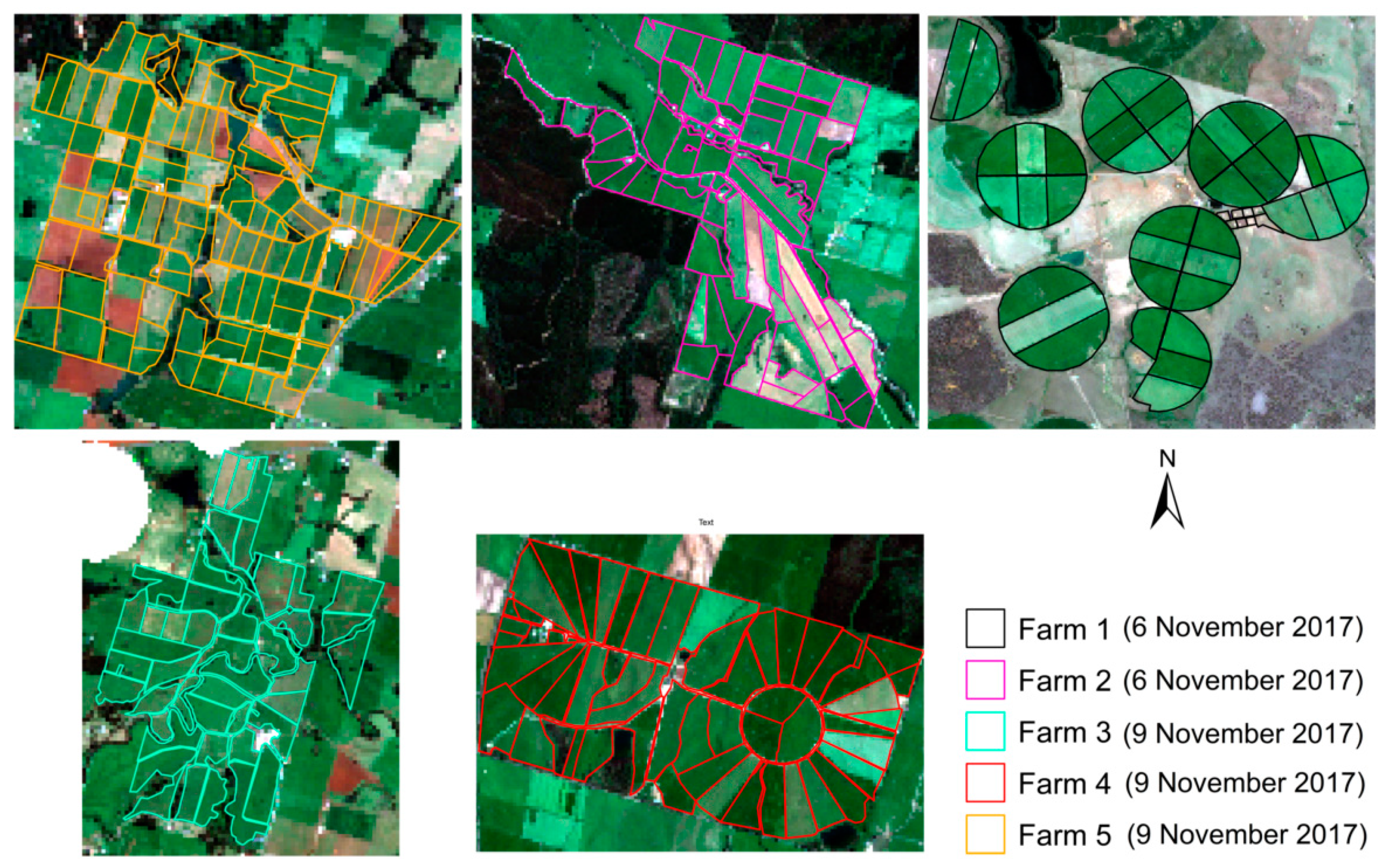
Figure 2.
Colour-composite images of Sentinel-2 bands 4, 3 and 2 (RGB) showing the five farms used as the study area.
Figure 2.
Colour-composite images of Sentinel-2 bands 4, 3 and 2 (RGB) showing the five farms used as the study area.

Figure 3.
Number of cloud-free and cloud-affected S2 images in each month in the five farms under study.
Figure 3.
Number of cloud-free and cloud-affected S2 images in each month in the five farms under study.

Figure 4.
Availability of in situ daily biomass measurements (kg DM/ha) and S2 images at the farm level (2017–2018). Circles indicate the median biomass for all paddocks in the farm: red indicates that a corresponding S2 image was available and blue indicates that a corresponding S2 image was unavailable; green squares indicate the S2-derived median NDVIs for all paddocks in the farm.

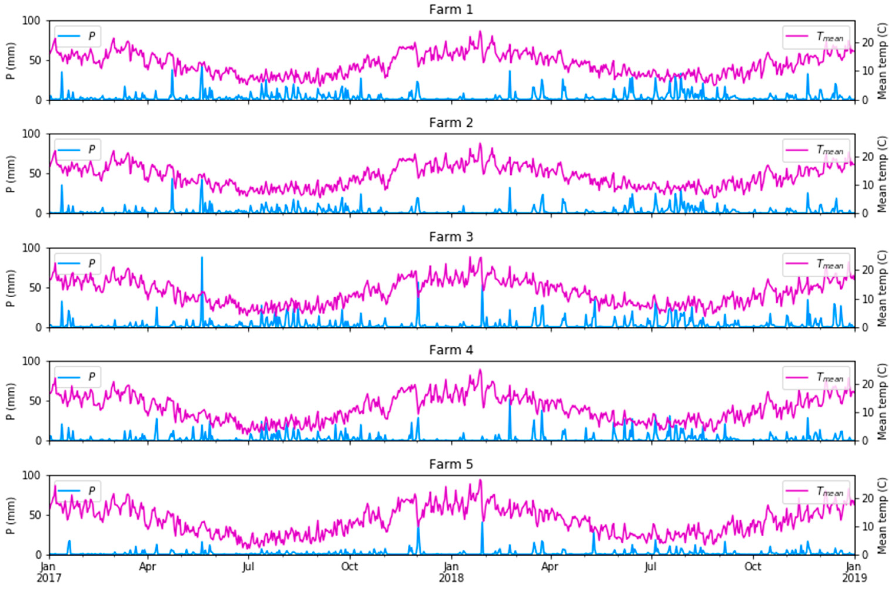
Figure 5.
Daily precipitation and mean temperature (Tmean = (Tmax + Tmin)/2) in the five farms under study.
Figure 5.
Daily precipitation and mean temperature (Tmean = (Tmax + Tmin)/2) in the five farms under study.

Figure 6.
Indicative architecture of the multilayer perceptron neural network model used in this study.
Figure 6.
Indicative architecture of the multilayer perceptron neural network model used in this study.

Figure 7.
Relationship between the ground-measured biomass (kg DM/ha) and the S2-derived NDVI for the five farms. Each point represents the median NDVI for all pixels in the paddock and the biomass measured on each day.
Figure 7.
Relationship between the ground-measured biomass (kg DM/ha) and the S2-derived NDVI for the five farms. Each point represents the median NDVI for all pixels in the paddock and the biomass measured on each day.

Figure 8.
Observed vs. predicted biomass (kg/ha) for the calibration (left) and evaluation (right) from the two experiment cases (n is number of samples). Top: Experiment 1 (S2 imagery only). Bottom: Experiment 2 (S2 imagery and climate variables).
Figure 8.
Observed vs. predicted biomass (kg/ha) for the calibration (left) and evaluation (right) from the two experiment cases (n is number of samples). Top: Experiment 1 (S2 imagery only). Bottom: Experiment 2 (S2 imagery and climate variables).

Figure 9.
Observed vs. predicted biomass for the sensitivity analysis. In each line, data from one farm was removed from the dataset used in the calibration (left), and the resulting model was tested on that farm (right). The model used included data from S2 and the climate variables (experiment 2).

Figure 10.
Box plots showing the temporal changes (October 2015–December 2019) of the estimated and observed biomasses in the five farms in each month. Each box plot shows the median, interquartile range (box) and maximum and minimum (whiskers) of all paddocks on the farm in the month.
Figure 10.
Box plots showing the temporal changes (October 2015–December 2019) of the estimated and observed biomasses in the five farms in each month. Each box plot shows the median, interquartile range (box) and maximum and minimum (whiskers) of all paddocks on the farm in the month.


Table 1.
Summary of the input data/variables from five farms in the study area (2017–2018).
| Data | Variable | Description |
|---|---|---|
| Field samples (once a week) | Biomass (kg DM/ha) | Paddock-based records from RPM or C-Dax |
| S2 imagery (20 m) (matching field sampling date with a maximum of two days before or after) | Band 2 | Blue (460–520 nm), resampled from 10 m |
| Band 3 | Green (540–580 nm), resampled from 10 m | |
| Band 4 | Red (650–680 nm), resampled from 10 m | |
| Band 5 | Red-edge-1 (700–710 nm) | |
| Band 6 | Red-edge-2 (730–750 nm) | |
| Band 7 | Red-edge-3 (770–790 nm) | |
| Band 8 | NIR-1 (780–900 nm), resampled from 10 m | |
| Band 8A | NIR-2 (860–880 nm) | |
| Band 11 | SWIR-1 (1570–1660 nm) | |
| Band 12 | SWIR-2 (2100–2280 nm) | |
| Month | Image acquisition month | |
| NDVI | Normalised difference vegetation index = (band 8 − band 4)/(band 8 + band 4) | |
| Climate data (5 km) (mean of 28 days before field sampling date, see Section 2.2.3 for an aggregation rationale) | P (mm) | Precipitation |
| RAD (W/m2) | Solar radiation | |
| Tmax (°C) | Maximum temperature | |
| Tmin (°C) | Minimum temperature | |
| Tmean (°C) | Mean temperature (Tmean = (Tmax + Tmin)/2) | |
| VPH-09 (hPa) | Vapour pressure deficit at 9 am | |
| VPH-15 (hPa) | Vapour pressure deficit at 3 pm |
DM: dry matter, RPM: rising plate meter, S2: Sentinel-2, NIR: near infrared, SWIR: shortwave infrared.
Table 2.
Summary of the farm characteristics, field biomass data and satellite imagery used in this study. The imagery figures show the number of in situ records that had a cloud-free S2 overpass within one day of the biomass measurement.
Table 2.
Summary of the farm characteristics, field biomass data and satellite imagery used in this study. The imagery figures show the number of in situ records that had a cloud-free S2 overpass within one day of the biomass measurement.
| Farm | Farm Area (ha) | Paddock | Mean Paddock Area (ha) | Start Date | End Date | In Situ Records | Concurrent S2 Imagery | Mean Biomass (kg/ha) | Std Dev Biomass (kg/ha) |
|---|---|---|---|---|---|---|---|---|---|
| 1 | 201 | 115 | 1.7 | 2017-01-04 | 2018-10-17 | 5779 | 635 | 2231 | 497 |
| 2 | 124 | 48 | 2.6 | 2017-01-02 | 2017-12-18 | 1951 | 193 | 2438 | 566 |
| 3 | 258 | 66 | 3.9 | 2017-01-04 | 2017-12-21 | 1212 | 123 | 2114 | 550 |
| 4 | 304 | 59 | 5.1 | 2017-01-04 | 2017-12-19 | 1720 | 421 | 2232 | 648 |
| 5 | 446 | 46 | 9.7 | 2017-04-04 | 2018-07-05 | 1685 | 361 | 2375 | 517 |
| Total | 1333 | 334 | 4.6 (mean) | 12,356 | 1735 | 2272 | 547 |
Table 3.
Summary of the model calibration, evaluation and sensitivity analysis.
| Item | Experiment (E) | Sensitivity (S) | ||||||||||||
|---|---|---|---|---|---|---|---|---|---|---|---|---|---|---|
| E1 (All Farms) | E2 (All Farms) | S (Farm 1) | S (Farm 2) | S (Farm 3) | S (Farm 4) | S (Farm 5) | ||||||||
| Cal * | Val ** | Cal | Val | Cal | Val | Cal | Val | Cal | Val | Cal | Val | Cal | Val | |
| N *** | 1300 | 433 | 1300 | 433 | 1098 | 635 | 1540 | 193 | 1610 | 123 | 1312 | 421 | 1372 | 361 |
| R2 | 0.51 | 0.50 | 0.62 | 0.57 | 0.65 | 0.44 | 0.68 | 0.22 | 0.67 | 0.32 | 0.63 | 0.22 | 0.68 | 0.40 |
| RMSE (kg/ha) | 406 | 403 | 356 | 366 | 360 | 521 | 324 | 598 | 327 | 462 | 328 | 655 | 331 | 436 |
* Cal: calibration; ** Val: evaluation; *** N: number of samples.
Publisher’s Note: MDPI stays neutral with regard to jurisdictional claims in published maps and institutional affiliations. |
© 2021 by the authors. Licensee MDPI, Basel, Switzerland. This article is an open access article distributed under the terms and conditions of the Creative Commons Attribution (CC BY) license (http://creativecommons.org/licenses/by/4.0/).
Share and Cite
MDPI and ACS Style
Chen, Y.; Guerschman, J.; Shendryk, Y.; Henry, D.; Harrison, M.T. Estimating Pasture Biomass Using Sentinel-2 Imagery and Machine Learning. Remote Sens. 2021, 13, 603. https://doi.org/10.3390/rs13040603
AMA Style
Chen Y, Guerschman J, Shendryk Y, Henry D, Harrison MT. Estimating Pasture Biomass Using Sentinel-2 Imagery and Machine Learning. Remote Sensing. 2021; 13(4):603. https://doi.org/10.3390/rs13040603
Chicago/Turabian StyleChen, Yun, Juan Guerschman, Yuri Shendryk, Dave Henry, and Matthew Tom Harrison. 2021. "Estimating Pasture Biomass Using Sentinel-2 Imagery and Machine Learning" Remote Sensing 13, no. 4: 603. https://doi.org/10.3390/rs13040603
Note that from the first issue of 2016, this journal uses article numbers instead of page numbers. See further details here.