Article

Multi-Source EO for Dynamic Wetland Mapping and Monitoring in the Great Lakes Basin

1
Michigan Tech Research Institute, Michigan Technological University, Ann Arbor, MI 48105, USA
2
Environment and Climate Change Canada, Ottawa, ON K1A 0H3, Canada
3
Natural Resources Canada, Ottawa, ON K1S 5K2, Canada
4
Minnesota Department of Natural Resources, St. Paul, MN 55155, USA
5
SharedGEO, St. Paul, MN 55104, USA
6
Department of Forest Resources, University of Minnesota, St. Paul, MN 55108, USA
7
Polar Geospatial Center, University of Minnesota, St. Paul, MN 55108, USA
*
Author to whom correspondence should be addressed.
Remote Sens. 2021, 13(4), 599; https://doi.org/10.3390/rs13040599
Submission received: 30 November 2020 / Revised: 30 January 2021 / Accepted: 3 February 2021 / Published: 8 February 2021
(This article belongs to the Special Issue Wetland Landscape Change Mapping Using Remote Sensing)

Abstract

:
Wetland managers, citizens and government leaders are observing rapid changes in coastal wetlands and associated habitats around the Great Lakes Basin due to human activity and climate variability. SAR and optical satellite sensors offer cost effective management tools that can be used to monitor wetlands over time, covering large areas like the Great Lakes and providing information to those making management and policy decisions. In this paper we describe ongoing efforts to monitor dynamic changes in wetland vegetation, surface water extent, and water level change. Included are assessments of simulated Radarsat Constellation Mission data to determine feasibility of continued monitoring into the future. Results show that integration of data from multiple sensors is most effective for monitoring coastal wetlands in the Great Lakes region. While products developed using methods described in this article provide valuable management tools, more effort is needed to reach the goal of establishing a dynamic, near-real-time, remote sensing-based monitoring program for the basin.

Graphical Abstract

1. Introduction

The Great Lakes Basin is the largest surface freshwater reserve on Earth, containing about 90 percent of North America’s and 20 percent of the Earth’s surface fresh water. As the nexus between land and the lakes, the coastal wetlands of the region are relatively small, comprising less than 1% of the area of the basin. Although they have a small spatial extent, their size is disproportionate to the significant role they play in the overall health of the Great Lakes system. Located between the United States of America and Canada, these wetlands provide significant services to both countries including water filtration, protection against erosion, and a variety of ecosystem services [1]. Additionally, they provide habitat and breeding grounds for myriad of birds, mammals, herptiles, and invertebrates [2]. The ecological and economic importance of the coastal wetlands of the Great Lakes was long neglected and anthropogenic activity has resulted in the loss of over half of the basin’s wetlands since European settlement [3,4]. More recently, their significance has been recognized and plans have been implemented at local, regional, and federal levels to protect the Great Lakes and their wetlands. The governments of the USA and Canada have both initiated large-scale efforts to protect the lakes and adjacent ecosystems with the Great Lakes Restoration Initiative (GLRI) and the Great Lakes Protection Initiative (GLPI) respectively [5,6]. Cooperative agreements between the two countries such as the Great Lakes Water Quality Agreement (GLWQA), among others, contain explicit language expressing the need to monitor and maintain coastal wetlands [7].
In practice, monitoring coastal wetlands is a huge challenge. In spite of their small total area, the coastline of the Great Lakes spans about 17,000 km. This length includes vast stretches of difficult-to-reach shoreline, making in situ monitoring across the basin an extremely difficult task. The Great Lakes Coastal Wetland Monitoring Plan (GLCWMP), funded by the GLRI, aims to do exactly that, and includes protocols for monitoring approximately 1100 coastal wetlands across the basin. The GLCWMP’s sampling protocols include rigorous collection of important data on water chemistry, plants, fish, birds, and macrophytes [8]. Because of the immense scope of the endeavor, each wetland is scheduled to be sampled once every five years. The Great Lakes and their associated wetlands are dynamic by nature and are especially susceptible to climate change and anthropogenic activity. Recently, rapid shifts in lake levels have occurred with record low levels in 2013 transitioning to record high levels in 2019 and 2020 [9]. Seasonally, Great Lakes water level fluctuations (on average ~30–40 cm per season) commonly exceed those encountered along marine shorelines including significant storm surge events [10]. Invasive species such as Phragmites australis and Typha × glauca provide further complications, as they are able to quickly invade and dominate native wetland plant species, especially in areas influenced by significant agricultural runoff [11]. The rapid changes observed in coastal areas presents unique challenges to Great Lakes wetland managers, regional and local governments leaders, and the public, requiring frequently updated spatial products to gain a synoptic view of their regions of interest. Remote sensing, while unable to directly measure what can be assessed in situ, is able to provide frequent information on wetland and surface water extent, water levels, and vegetation type.
Satellite and aerial images are essential, cost effective, and scientific-based management tools capable of tracking and observing wetland and associated habitat changes over time, covering large areas like the Great Lakes. Remote sensing techniques have been used to assess Great Lakes wetlands for several decades. With new sensors providing higher temporal and spatial resolution than ever before it has become easier to provide coastal wetland managers with timely and informative remote sensing derived products to aid in their efforts to protect the Great Lakes’ coastal zones. This article highlights the preliminary results of a bi-national collaboration to build on established remote sensing approaches to develop the framework for ongoing, high-frequency, high-resolution, remote sensing-based monitoring for Great Lakes coastal wetlands.
The overall goal of this collaborative effort is to develop semi-automated and automated methods for application of high-resolution satellite, multispectral and Synthetic Aperture Radar (SAR) imagery for monitoring various components of wetlands in preparation for an operational capability in the Great Lakes Basin. This includes wetland classification, surface water and flooded vegetation delineation, and estimation of water level measurements. This team of researchers aims to develop, demonstrate and plan the implementation of innovative approaches for using multi-sensor satellites to create wetland baselines and to estimate change over time. Further, it incorporates petascale computing capabilities to demonstrate the applicability of these approaches for the entire basin. The information gained will support the management of wetlands, as well as related environments and human activities.
Specific objectives of this monitoring effort include preparation for the operational implementation of dynamic surface water extent mapping techniques developed with RADARSAT Constellation Mission (RCM); refinement of methods for producing wetland classification and change including invasive vegetation and adjacent land cover by leveraging techniques such as object-based image analysis and machine learning; multi-temporal vegetation elevation and ecosystem modeling based on high-resolution stereo satellite imagery; and Interferometric Synthetic Aperture Radar (InSAR) water level monitoring.
This article presents a short background of remote sensing of wetlands in the Great Lakes and details the results of a survey of wetland managers which informed the development of specific geospatial products and how frequently they are produced. This paper is structured with a series of case studies which highlight examples of each of the products from areas of interest around the basin. The methods and results presented here demonstrate an initial framework for utilizing multi-source, multi-temporal, high resolution remote sensing data for dynamic coastal wetland monitoring in the Great Lakes Basin.

2. Background

Efforts to map Great Lakes wetlands have been ongoing for several decades. Programs such as the National Wetlands Inventory (NWI), administered by the U.S. Fish and Wildlife Service, began to create a spatial database of all U.S. wetlands starting almost four decades ago. The NWI maps are produced by teams of aerial image interpreters who detect and draw wetland boundaries using orthophotos. The NWI provides detailed data on wetland extent for most of the U.S. [12]. While being an incredibly useful resource, initial completion and subsequent updating of the NWI is a time-consuming process, with maps for some regions being over 30 years old or older. The Canadian Wetland Inventory, launched in 2002, was created to develop a similar inventory for Canada but remains incomplete for the Great Lakes region [13]. The National Oceanic and Atmospheric Administration’s Coastal Change Analysis Program, which relies on Landsat imagery and other ancillary information, provides more frequent updates at the expense of spatial resolution [14]. These programs generally target only one country, and few cohesive projects have completed a map of coastal Canada and the USA using a single method. Bourgeau-Chavez et al. [15] completed a binational map of Great Lakes coastal wetlands using data circa 2010 and updated it for areas with substantial Phragmites infestation with image data for 2017 [16]. While all these products are useful, they tend to portray a “snapshot” in time and fail to capture the dynamic nature exhibited by coastal areas in reality. Additionally, the maps tend to contain limited information on the wetlands themselves, often being limited to classification schemes based on general vegetation type.
Wetland managers and other stakeholders were interviewed by the research team in Spring 2017 to determine how satellite remote sensing could help meet their needs for real-time and long-term data. The purpose of the activity was to obtain first-hand input from potential end users of Great Lakes wetlands satellite products in order to maximize the practical value of those products. Phone surveys were conducted with 30 participants who were asked to discuss the usefulness of the various products being developed. Product usefulness ratings varied according to each respondents’ responsibilities, but aggregate ratings for each of four products were greater than 3 on a 0–5 scale (surface water extent—3.2, water level—3.6, land cover and land cover change—3.9, invasive species extent—4.9). Participants were also asked about the ideal frequency of each product, and with few exceptions, they expressed a desire to have annual or better frequency products. These results verified the need for more timely spatial products to aid in wetland management for the coastal Great Lakes.
A recent review of remote sensing for coastal wetland in the Great Lakes, White et al. [17] describe a variety of approaches for mapping and monitoring using a variety of sources including high resolution multispectral and SAR remote sensing techniques. These sensors are well suited for generating the products identified by resource managers. Multispectral data (including near-infrared (NIR) and shortwave infrared bands) are sensitive to variation in vegetation health and moisture content, which is of great importance in wetlands [18]. Synthetic Aperture Radar (SAR) is often used to map wetlands because it can capture imagery day or night and can penetrate cloud cover [19]. Research has shown that fully polarimetric (FP) SAR is better suited to mapping wetlands compared to single or dual polarimetric SAR, both of which are also available on RADARSAT-2 [20,21,22,23,24]. A recent meta-analysis of North American wetland remote sensing classification efforts found that multi-source data were comparable to the best results of single-source approaches [25]. The combination of SAR and multispectral data fuses the strengths of each sensor to provide the most powerful tool to monitor wetlands.

3. Materials and General Methods

A team of wetland remote sensing experts from across the basin was assembled to develop the basis for the dynamic monitoring protocols described here. Led by the United States Environmental Protection Agency (USEPA) and United States Fish and Wildlife Service (USFWS), the core team for this effort includes the University of Minnesota, Michigan Tech University, Minnesota Department of Natural Resources and SharedGeo. The National Science Foundation provided significant supercomputer support, while access to commercial satellite imagery was provided via National Geospatial-intelligence Agency (NGA) with MAXAR supplying both the optical and radar imagery.
Fourteen regions containing coastal wetland complexes were chosen as pilot sites from across the Great Lakes Basin to represent a range of hydrogeomorphic types with varying anthropogenic stressors. The pilot sites range from the largest freshwater delta of the St. Clair River to lacustrine systems of western Lake Erie and Long Point, lacustrine bays of Lake Huron (Les Cheneaux Islands, Saginaw Bay), Lake Ontario (Bay of Quinte), and Lake Michigan (Green Bay), riverine systems of Lake Superior (St. Louis River Estuary, Bad River) to barrier protected wetlands such as White Fish Point.
All optical imagery used for this research was acquired via the NGA NextView license, which includes high-resolution imagery from DigitalGlobe’s archives. Synthetic aperture radar imagery came from RADARSAT-2 via the Northern View agreement. SAR image collection are focused on the 14 pilot sites (Figure 1) while DigitalGlobe data continues to be acquired for the entirety of the basin (Table 1). RADARSAT-2 imagery is collected every 24 days from April–November for pilot sites. DigitalGlobe imagery is acquired less frequently, however, multiple cloud-free images have been acquired for most areas.
DigitalGlobe imagery includes the Worldview constellation, which is the primary source of multispectral data used for the effort described here. The satellite sensors comprising the WorldView Constellation all include visible and near-infrared bands with the exception of WorldView-1. WorldView-2 and -3 have additional shortwave infrared bands. These sensors have been used in a variety of wetland studies and have the potential to aid in accurate mapping of wetland type and extent at meter resolution [26,27].
RADARSAT-2 is a Canadian C-band SAR satellite and has been used in many wetland studies. Canada recently launched the RADARSAT Constellation Mission (RCM) in June 2018. RCM is also a C-band SAR and is capable of operating in a Compact Polarimetric (CP) mode. CP SAR does not have complete polarimetric information like FP [20] SAR but contains more information than single or dual polarimetric data. While the CP mode is not expected to be as accurate in mapping wetland classes and monitoring change due to reduced polarimetric information and a higher Noise Equivalent Sigma Zero (NESZ), it offers a wider swath width allowing for larger areas to be mapped simultaneously. In addition, RCM is a constellation of three identical satellites, so the same location can potentially be mapped more frequently (4-day overall revisit time, 12 days for individual satellites) [28,29]. While RCM data was not available at the time this work was completed, simulated RCM products derived from RADARSAT-2 were used in some cases. For SAR imagery, standard pre-processing procedures (calibration, speckle reduction, geometric correction) were applied using PCI Geomatica software in all cases.

4. Methods and Results

Methods for each objective are described as case studies in each of the following sections.

4.1. Dynamic Surface Water Extent Mapping

Climate change is expected to negatively impact a variety of environmental factors which are likely to include ambient temperatures, precipitation, and flow regimes [30]. Wetlands are vulnerable to these environmental shifts and even small changes in the duration of flooding and depth of water may cause [31,32] the loss of suitable habitat for species that are not able to adapt to new levels of variation and could lead to increased numbers of invasive and or generalist species [33]. In light of this, there is a need for regional monitoring of changes in the extent of surface water within wetlands as this will help identify those areas that are changing. Not only would this inform management strategies, but also focus conservation efforts, which will be especially beneficial to those species for which wetlands provide habitat and are already at risk of extinction.
Surface water detection (SWD) using SAR data has been the subject of study for many projects [34,35,36]. This is in large part because it is a reliable source of consistent information since images can be acquired regardless of cloud cover and haze. Further, due to predominant specular reflection, radar backscatter over non-disturbed water bodies is low relative to most surrounding land and other non-water features. This results in contrasting dark water features and relatively bright non-water features, a characteristic that can be used to discriminate both cover types in SAR images. Due to their simplicity, threshold-based methods are widely used for operational SWD, particularly for large datasets. Several techniques exist for finding an appropriate threshold value to distinguish between land and water [37,38,39,40].

4.1.1. Dynamic Surface Water Extent Mapping with RADARSAT-2

One of the first joint products the US-Canada team worked on was the development of an automated SWD technique for the Great Lakes [40]. To apply the published SWD technique described in [40] to the pilot sites of Figure 1, there have been some slight modifications which are described here. The automation has been applied to 254 RADARSAT-2 images, collected in FQ or FQW beam modes, to produce surface water extent maps (Table 2).
After standard pre-processing the HV component of each RADARSAT-2 image, expressed in dB, is then ingested and randomly subsampled (typically 10,000 pixels). A histogram is generated from the subsampled pixel values, and a polynomial fit is applied before the threshold between land and water is selected. The entire HV image is then segmented using the SLIC super pixel technique [41]. Each segment is assigned the value of its median pixel value and then determined to be land or water based on the previously determined threshold.
Many of the pilot sites contain significant urban areas (e.g., Green Bay, Duluth, Saginaw Bay). Observations of preliminary surface water extent products for these developed regions showed significant confusion between flat impervious surfaces, such as roads and runways, and water. As a side looking active sensor, incoming microwave energy is reflected specularly away from the sensor from smooth surfaces. This produces the typically observed low backscatter over water, but similar physical interaction between the SAR and man-made surface features is indistinguishable. Therefore, an additional step was adopted to apply an impervious surface mask to the output surface water extent maps. The impervious surface masks were generated using WorldView constellation data acquired via this project. One shortcoming of this approach is that it fails to identify real flooding that can occur over highways or runways following significant precipitation events, however, since the focus is on wetland monitoring those potential omission errors were deemed acceptable. Each RADARSAT-2 image is processed with this method, creating a surface water extent map for each date an image is acquired. Figure 2 shows an example of a surface water extent map, overlaid on an optical image, for July of 2017 for the St. Clair River Delta.
While this automated technique captures surface water in open areas, a second algorithm was needed to extract inundation beneath a vegetation canopy. The wetland inundation mapping uses the Shannon Entropy [42] metric, which can be calculated from dual-band or quad-pol SAR data. The algorithm has two outputs which represent contributions from intensity and polarimetry, and the intensity contribution is used. Separation of non-flooded and flooded vegetation is not feasible using histogram-based thresholding approach, so thresholds are selected based on in-situ measurements. Typically, values greater than 1 are classified as flooded vegetation. This method is preferable to three-component decomposition methods because it is not susceptible to inaccuracies due to misclassification of double-bounce scattering as single bounce in common marsh vegetation such as cattail [43].
Given the number of images available for the pilot areas, it is possible to assess relative hydroperiod at each location. Each image is classified as 1 = water/inundated or 0 = land. The images are then summed so each output pixel value represents the number of times that it was classified as water/inundated. The time series can be divided up in a variety of ways, but compiling surface water maps for each year has proved to be a valuable tool for visualizing interannual hydroperiod variability. Figure 3 shows relative hydroperiod for the St. Clair River Delta from 2016–2018.
Water levels have increased in Lake St. Clair over the past several years, and the effect of those rising lake levels can be seen in the relative hydroperiod maps. Pixels identified as being water/inundated for every image in a year increased from 40.6% in 2016 to 45.9% in 2018. Perhaps even more interesting is the increase in number of pixels identified as water/inundated at least once within each year. This number increased from 60% in 2016 to 74% in 2018. This represents an over 70 km2 of area that is classified as being inundated at some point during the growing season. This rapid increase in water extent highlights the importance for continued monitoring of coastal areas.

4.1.2. Dynamic Surface Water Extent Mapping in Preparation for RCM

Since there is a need to transition the SWD approach of Radarsat-2 to the RCM, simulated RCM data for the Bay of Quinte was analyzed. The study area is located on the northern shore of Lake Ontario, Canada, commonly referred to as the Bay of Quinte (Figure 1). It includes the entire island of Prince Edward County, as well as Belleville and Greater Napanee. The climate can be described as cold and temperate, with substantial rainfall throughout the year (902 mm on average), peaking in September (90 mm on average) [44,45]. The wetlands in this region are home to a variety of plants and animals, including numerous species at risk. They also provide important nesting and stopover habitat for waterfowl [46]). It encompasses a variety of different wetlands, including large ones which are permanently flooded, and smaller ones which are only flooded for a portion of the season. The extent of water bodies varies extensively on an inter and intra-annual basis, both as a result of water level changes, and the emergence of vegetation from the water surface as the growing season progresses [36,37,38].
For this site, multiple RADARSAT-2 images were acquired between 27 April and 22 September 2016. Simulated RCM data was generated for one date only, for the beam mode FQ17W (27 April). The image covers approximately 50 × 50 km2 area, and consists of two 50 × 33 km2 frames with a nominal near range resolution of 8.9 m. The main reason for selecting the scene on this date is that the emerging vegetation is relatively minimal in April/May. Behnamian et al. [40] showed that the thresholding-based SWD methods have limited capabilities in detecting emerging vegetation until it becomes dense (and tall) enough to affect the backscatter of the incident microwaves and as a result the shape of the histograms. This is a lesser concern in the beginning of the growing season.
Both quad pol RADARSAT-2 images were processed to projected RCM specifications using the Canada Centre for Mapping and Earth Observation (CCMEO) simulation software [39]. Note that the same processing chain as outlined by White et al. and Banks et al. [38,40] is applied here, where RADARSAT-2 data is first converted from the scattering matrix to the Kennaugh matrix. Values are then multiplied by a Stokes vector representing a right-hand circular polarized wave, to which a NESZ pattern was added to the first element to emulate the radiometric data quality of a given RCM beam mode. A 5 × 5 boxcar filter was applied to reduce the effects of speckle. RCM NESZ values vary from −25 dB for medium resolution mode to −19 dB for high resolution mode. It is worth noting the swath width of the FQW mode of RADARSAT-2 is 50 km, while the swath width of the high and medium (16 m) resolution modes of RCM are 30 km. This means that the simulated RCM will not have the right noise level for 10 km at the near and far range of each swath. Thus, these data are excluded from our analysis. Figure 4 shows an example of such unrealistic noise levels at the edges of the simulated RCM data in the FQ17W mode. We anticipate that these values would have affected both the distribution of values and thus were not used for the calculation of threshold as described in Section 4.1.1 above.
Thresholds for SWD were generated from linearly polarized (HH, HV) RADARSAT-2 and compact polarized (RH, RR) simulated RCM data at two different noise floors (−19 and −25 dB) over both study areas. It is important to point out that the NESZ values listed in Table 3 are the highest values that are usually located on the (near or far) edges of the RCM products and that the exact values of the noise floor are also a function of incidence angle of the RCM data. Table 3 shows the value of thresholds from the simulated RCM data (using FQ17W mode image) over the Bay of Quinte. At this incident angle, all simulated polarizations show bimodality, thus, threshold values were calculable. However, for the HV polarization, the threshold values for the −19 dB NESZ data were not reported since they were below the noise floor and thus not meaningful. With the HH polarized data, the threshold values were 4 dB larger than −19 dB NESZ.
The thresholds calculated from the compact polarimetric images were closer to the noise floor in the high-resolution mode, and as a result, the surface water products generated from these data could be potentially affected by noise (i.e., the predicted extent of surface water could be unreliable in cases where the thresholds are at or near the noise floor). The noise rms (which in general is a function of theoretical values per beam mode and the antenna theoretical directivity patterns in this case is within 1 dB. For the medium resolution simulated data, the calculated threshold values are at least 4 dB greater than the NESZ value for all polarizations and thus less likely to be affected by the noise pattern and noise rms.
It should be noted that some sample RCM images acquired in winter 2019 in high-resolution mode suggest that the noise floor is generally better than the official NESZ specification of RCM (2 to 4 dB in some cases), which may make it possible for the users to use compact polarimetric modes for surface water detection. In this study, we have not investigated the incident angle effects on the threshold values using simulated data as the steeper incident angles are more sensitive to wind effects, causing Bragg-scale waves formed in response to wind stress over water surface resulting in stronger backscatter over water and affecting the bimodality of the histograms, thus it will make it more difficult to separate the effects of noise floor from wind effects.
Results demonstrate that at the incidence angles that were evaluated, the thresholds calculated for SWD from simulated RCM data are not close to the noise floor in medium-resolution mode for HH, HV and CP polarizations and thus can be used for SWD. With high-resolution mode RCM data, the results suggest that the thresholds calculated from the HH polarization are well above the noise floor. However, this was not the case for the HV and compact polarizations. The Emergency Geomatics Service at CCRS/CCMEO, which has the mandate for flood response mapping for the Government of Canada, have reported no noise floor problems when using the RCM dual-polarization data for surface water mapping [47].

4.2. Wetland Classification and Change Detection

Land cover maps provide users with a bird’s eye view of the various ecotypes present within a region of interest and can include information on wetland type and extent. Depending on the temporal, spatial, and class-level detail required for various management and monitoring efforts, different types of classification approaches may be utilized. For example, products that depict wetland status at the regional scale, required by agencies such as USFWS or ECCC, do not require the level of detail that would be needed for local management of waterfowl habitat within a particular wildlife preservation area. As such, several approaches for generating classified wetland maps are presented in the following sections.

4.2.1. Multi-Sensor, Multi-Temporal Approach

Highly detailed maps are sometimes necessary for monitoring specific wetland plant species, such as the invasive Phragmites australis and Typha spp., which have colonized vast expanses of coastal Lake Huron, Lake Erie, and Lake Michigan. Millions of dollars have been spent attempting to control Phragmites in the Great Lakes region [48]. Saginaw Bay, located within the state of Michigan, has been especially hard hit, with monotypic stands over one-kilometer-wide stretching along the southern and eastern coasts of the bay. Significant efforts to control the invasive stands with combinations of mowing, burning, and chemical treatment have occurred within the last several years. Remote sensing-based monitoring leveraging the multi-sensor, multi-temporal approach have been implemented with high-resolution imagery available from the WorldView constellation and RADARSAT-2.
The general procedure for creating such maps, outlined in [15], involves using training data, typically generated by image interpreters using high resolution aerial or satellite images, and validation data, gathered in the field via a stratified random sampling approach, to classify an image stack using the Random Forests classifier [49]. This method has been utilized for grasslands, boreal peatlands, and tropical alpine peatlands as well [50,51,52] and tends to produce maps with overall accuracy above 85%. Utilization of RADARSAT-2 data, which has approximately 6 cm wavelength as opposed to the 24 cm wavelength of L-band SAR, limits the feasibility of mapping higher biomass woody wetland types because the shorter wavelength of C-band SAR does not have the same ability to penetrate canopy as L-band, though careful selection of incidence angle and image capture date can produce adequate accuracies (see Section 4.2.3). The limitations in mapping woody wetlands are outweighed by the ability to identify some leading edges of invasive Phragmites, which can overtake vast coastal wetland complexes in short order.
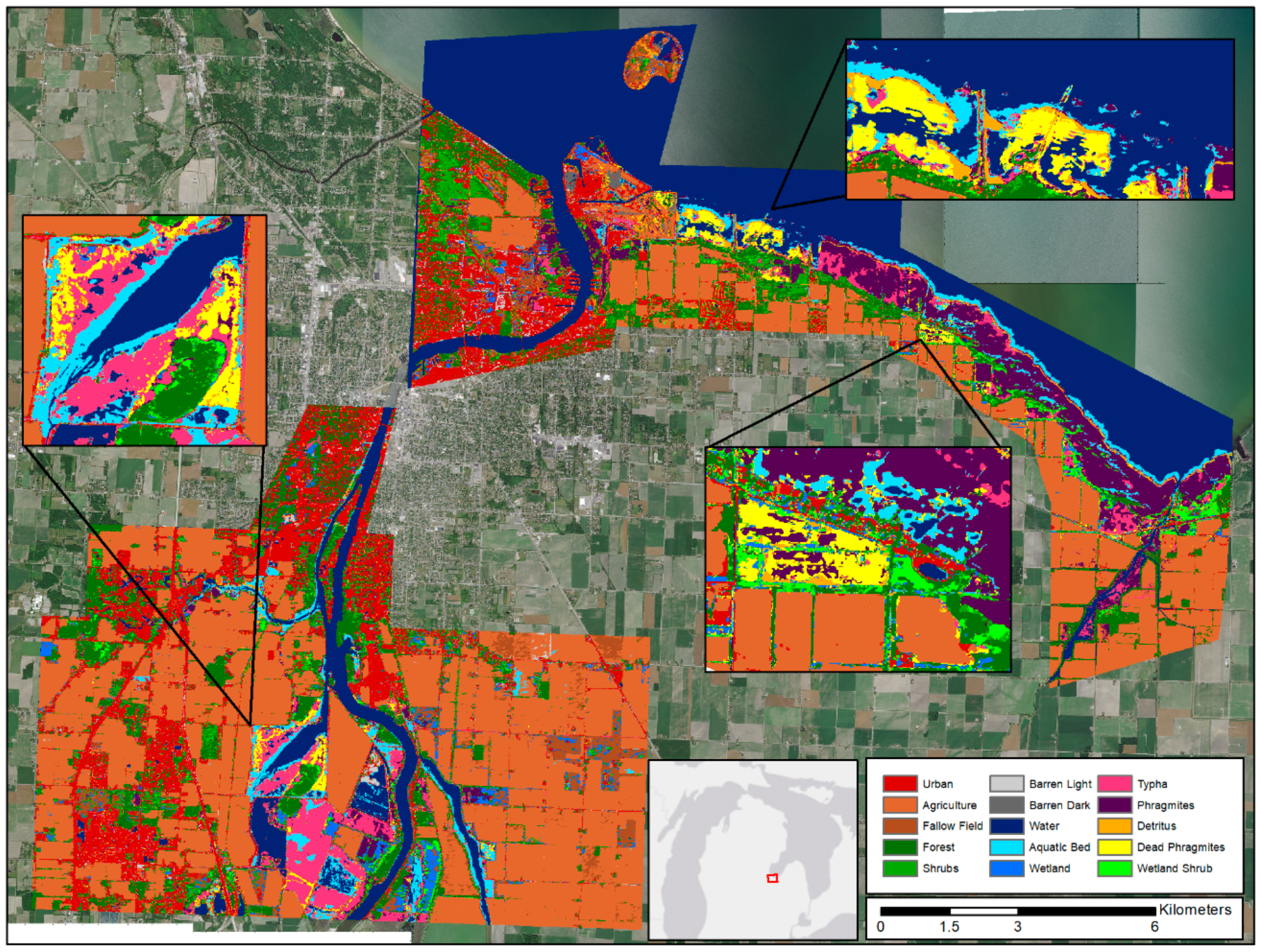
A 2018 classification using a Worldview-2 mosaic and multi-temporal Radarsat-2 imagery was generated for Saginaw Bay, MI. A mosaic of 17 May, 1 July, 14 August, 5 September 2018 Worldview-2 and 31 May, 18 July, 4 September 2018 Radarsat-2 imagery used for classification. RADARSAT-2 images were all collected in FQ10W mode, which provides FP data, were calibrated to sigma naught, speckle filtered using a 5 × 5 boxcar filter, and terrain corrected using PCI Geomatica software. Validation data were collected during several field visits conducted during the summer of 2018, and training data were generated by inspecting the WorldView-2 imagery and digitizing training polygons.
The output map (Figure 5) has 78% overall accuracy, with high accuracies for targeted wetland classes. Phragmites (PA = 91%, UA = 75%), Dead Phragmites (PA = 81%, UA = 83%), and Typha (PA = 93%, UA = 94%) were all generally accurate, providing a high-resolution, recent baseline map for managers to use to assess the efficacy of various Phragmites control measures. Significant treatment occurred between 2016 and 2018, so where data was available, maps could be created for both time periods and analyzed for change. 
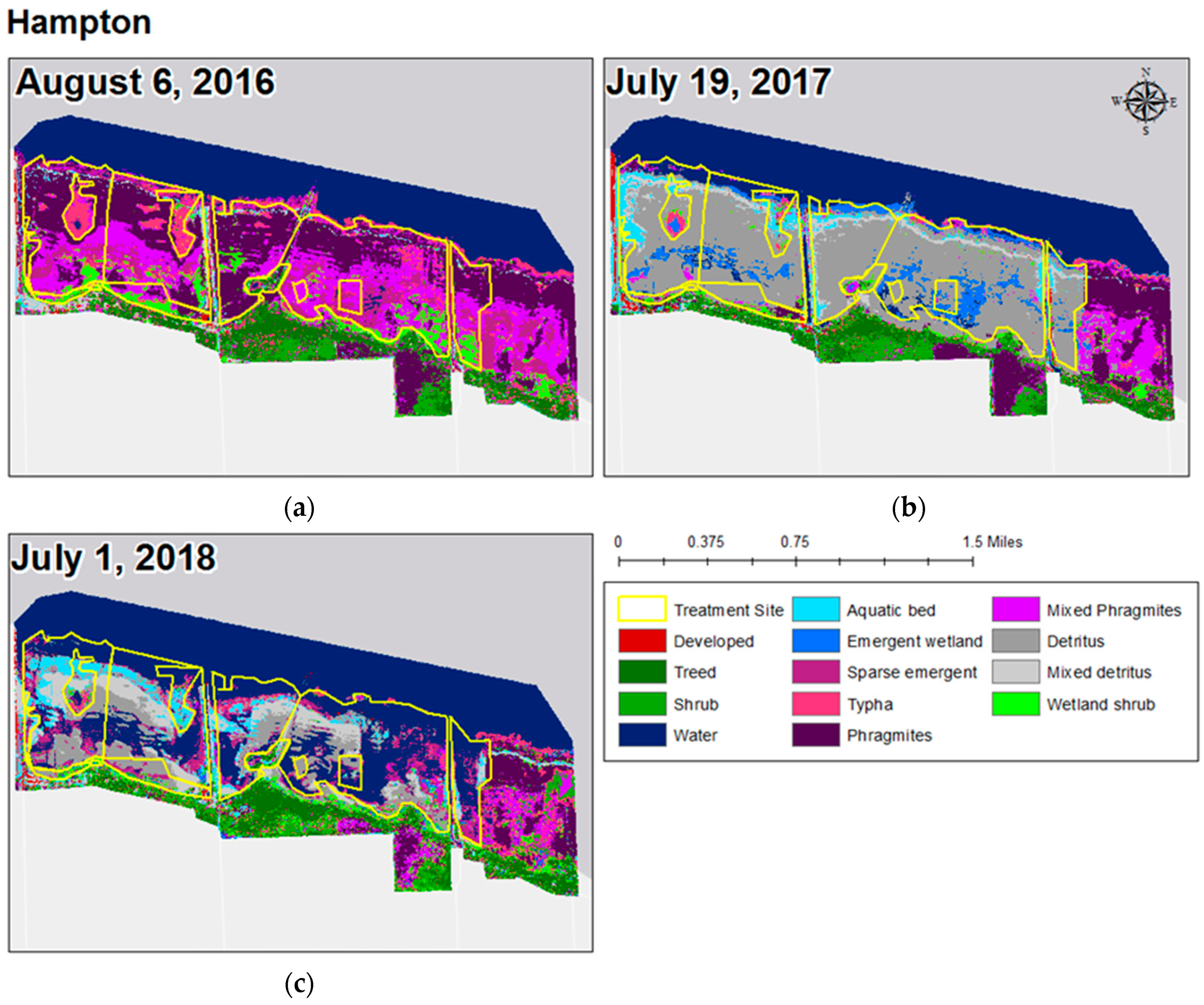
Figure 6 shows an example of the Hampton area in Saginaw Bay. By summer of 2016, the site was infested with Phragmites, which had taken over native wet meadows and emergent vegetation. The area was treated with a combination of glyphosate and imazapyr in Fall of 2016 and was later partially mowed in the winter of 2017.
These maps were produced from Worldview-2 imagery alone in Random Forests at very high resolution (sub-meter) and are being used by the Saginaw Bay Cooperative Invasive Species Management Area (SB-CISMA) and other stakeholders in applying an adaptive management strategy to the control of invasive Phragmites. The team cut out the agricultural areas and most non-wetland to produce these maps quickly based on the field data collected in transects within the treatment sites and image interpretation. A total of 11 treatment areas have been monitored using the remote sensing approach described here to augment field visits. Table 4 shows the results of the remote sensing-based monitoring approach, showing the change in Phragmites extent for each treatment location.
Treatment efficacy varied from site to site, but the results show an overall decrease of 89% of total infestation area 1–3 years post-treatment. Continued remote sensing-based monitoring will help provide managers with the ability to assess treatment types to develop optimal protocols to limit Phragmites expansion and decrease overall Phragmites coverage.
While the multi-temporal, multi-sensor approach generally produces the most accurate, high-resolution products that can distinguish wetland vegetation at the species level, it is not ideal for all circumstances. The process is time consuming, as it requires significant human input in the form of high-quality training and validation data. The use of multi-temporal data, while helpful for identifying subtle changes in phenology that can differentiate vegetation type, reduces the ability to detect short-term changes. An object-based image analysis (OBIA) approach is being utilized to address some of these limitations.

4.2.2. OBIA Classification Approach

An OBIA approach using expert knowledge and high resolution remotely-sensed data was applied to generate accurate map products of the Great Lakes coastal landscape and to provide a baseline for monitoring changes in these coastal regions. This approach has been used for mapping geomorphic landforms [53], urban infrastructure [54], wetlands [55], and surface waters [56] and expands on existing wetland and landscape mapping efforts, such as that described in Section 4.2.1, by leveraging sub-meter resolution stereo pairs acquired by DigitalGlobe/MAXAR and digital surface models (DSM) derived from these images. The DSMs provide height information for separating vegetation into various height strata and communities such as forest and scrub/shrub. Successfully classified image objects contain attributes that label a given feature, e.g., forest, and includes the spatial extent, height, and observation date from the imagery. Wetland and upland vegetation features include detailed attributes for vegetation height, extent, community, and the spatial neighborhood relationship to other land cover features.
The image object attributes based on the imagery bands and spectral indices such as normalized difference vegetation index (NDVI) were used to classify the imagery into water and land features. Water was identified using thresholds on low near-infrared (NIR) values and NDVI. The remaining unclassified areas represent land features; these features were segmented again to separate non-vegetated features using low NDVI values from vegetated features using high NDVI values. The low NDVI values (NDVI < 0) used for identifying non-vegetated features successfully classified urban infrastructure such as roadways, parking structures, buildings, and barren areas such as exposed rock formations. The vegetation class was further refined using the DSM and associated height values to map different vegetation communities.
Stereo-derived DSMs were used in this project to map features based on height values. Stereo image pairs were used to create DSMs for each satellite image pair. The DSMs represent the height of features above WGS84 Ellipsoid. We compared the DSMs to lidar-derived DSMs and discovered a vertical offset between the stereo-derived and lidar-derived DSMs. This vertical offset needed to be accounted for to compare DSMS across different image acquisitions. The vertical offset was constant across the stereo DSM scene but arbitrary in value. To address this issue, we align the stereo-derived DSM results to known ground reference points in the NAVD88 vertical datum. The reference points that were used must be dispersed across each scene and occur in open areas (open fields, along roadways, other open areas). Where lidar data was available, the bare-earth DEM was used to adjust the stereo-derived DSMs to align directly with the lidar DEM. Reference points under closed canopy, near buildings, or near water were removed to avoid misalignment. For areas that did not have lidar data, we used National Geodetic Survey (NGS) points to adjust for the vertical offset. The NGS are well-distributed spatially but less ideal because there are fewer points and many occur on roadways. The adjusted DSMs were normalized prior to being incorporated into the OBIA process.
The DSMs were normalized so that elevation values in the layer represent the height of features relative to the ground. The adjusted DSMs were normalized using lidar-derived DEMs or leaf-off stereo-derived DSMs to produce normalized digital surface models (nDSM). The lidar-derived normalized nDSM was created by subtracting the DSM from the DEM. In areas lacking lidar data, we used adjusted leaf-off DSMs as the DEM to create nDSMs. The leaf-off DSMs were found to closely represent terrain in areas with non-woody stem vegetation or deciduous canopy cover. We used leaf-off DSMs acquired during the same year or within one year of the DSM’s acquisition date to create the nDSMs by subtracting the leaf-on DSM from the leaf-off DSM. The resulting nDSMs were an essential data layer for classifying the vegetation height classes and their associated communities using an OBIA approach.
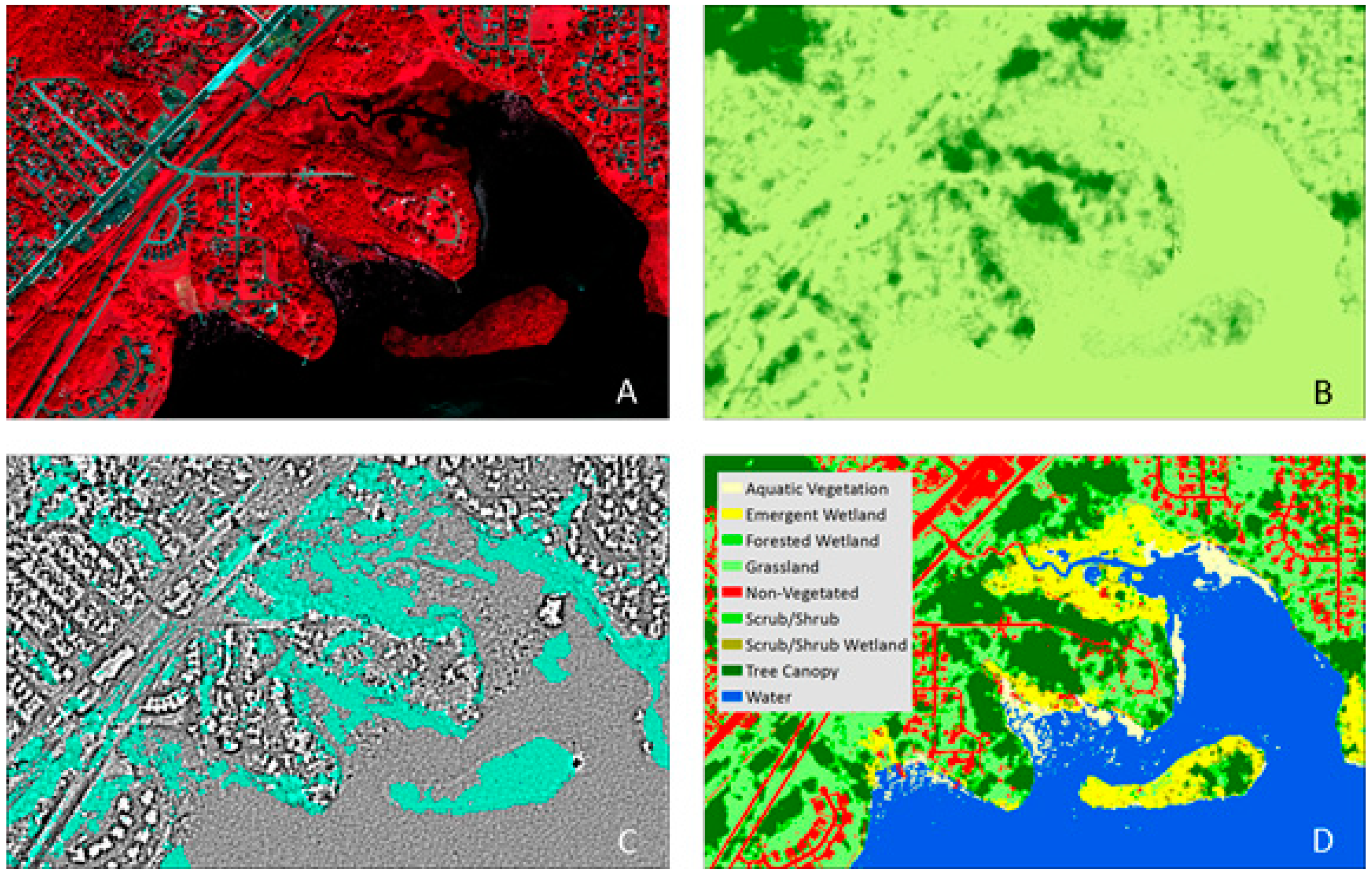
The OBIA approach integrated the imagery and nDSMs to map nine land cover classes: low vegetation, medium vegetation, tall vegetation, water, non-vegetated, aquatic vegetation, and emergent, scrub/shrub, and forested wetland (Figure 7). The water class was mapped using the optical data and low NIR values (<100). Non-vegetated areas were mapped using low NDVI values (<0) while vegetation classes were mapped using high NDVI values (>0) and height thresholds for low (<2 m), medium (<5 m), and tall (>5 m). These vegetation classes were then used as the basis for mapping wetland classes. Wetland areas within the classification were identified by using a threshold of the topographic position index (TPI). TPI is a layer derived from a DEM that is useful for identifying depressional features (e.g., wetlands). These depressions combined with wetland data mapped by MTRI allowed us to divide the vegetated classes into upland and wetland classes. Low vegetation within a wetland was classified as emergent wetland, medium vegetation was classified as scrub/shrub, and tall vegetation was classified as forested wetland. Aquatic vegetation or floating vegetation was mapped by comparing changes in the land cover classes between different dates of imagery acquisition.
Change detection was performed by comparing the wetland classifications from different dates to produce gain, loss, and no change wetland layers (Figure 8). The classification was stored as vector polygons with class and extent attributes. The classified image objects from one date were intersected with the classified image objects from a different date. If the class in all or a portion of an image object matches the intersecting class of another image object, the area is reclassified as no change. If the intersecting image object class covers a lower areal extent, it is reclassified as loss while an intersecting image object class with a larger areal extent is reclassified as gain. This comparison enabled us to identify aquatic or floating vegetation by labeling water objects that changed to vegetation objects as aquatic vegetation. We compared the classifications for the Duluth area based on WorldView3 (DigitalGlobe) optical data and derived DSMs acquired in April, June, and August 2016. While the comparison showed very little change between most land cover classes, we found that the extent of the aquatic vegetation doubled in area from 4.5 ac to 9.6 ac between June and August 2016.
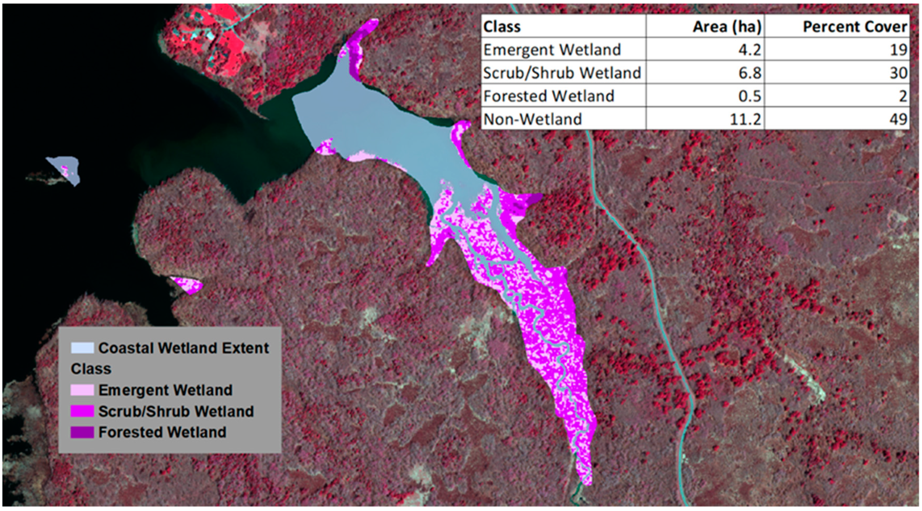
The OBIA approach was applied to a larger spatial extent using the Great Lakes Coastal Wetland Inventory (GLCWI) from the Great Lakes Coastal Wetland Consortium (https://www.glc.org). The approach integrated the multispectral imagery, DSMs, and lidar-derived DEMs to create forested, scrub/shrub, and low vegetation classes using multiple height thresholds: Forested (>2 m), scrub/shrub (0.5 m < 2 m), and low vegetation (<0.5 m). The GLCWI polygons were used to summarize the vegetation classes in each polygon as forested, scrub/shrub, and emergent wetland classes. While the areal extent of each wetland polygon was used to summarize the area (ha) and percent cover for each class (Figure 9). The OBIA process was readily transferable to each scene and used to batch process the Western Lake Superior region imagery (n = 622).
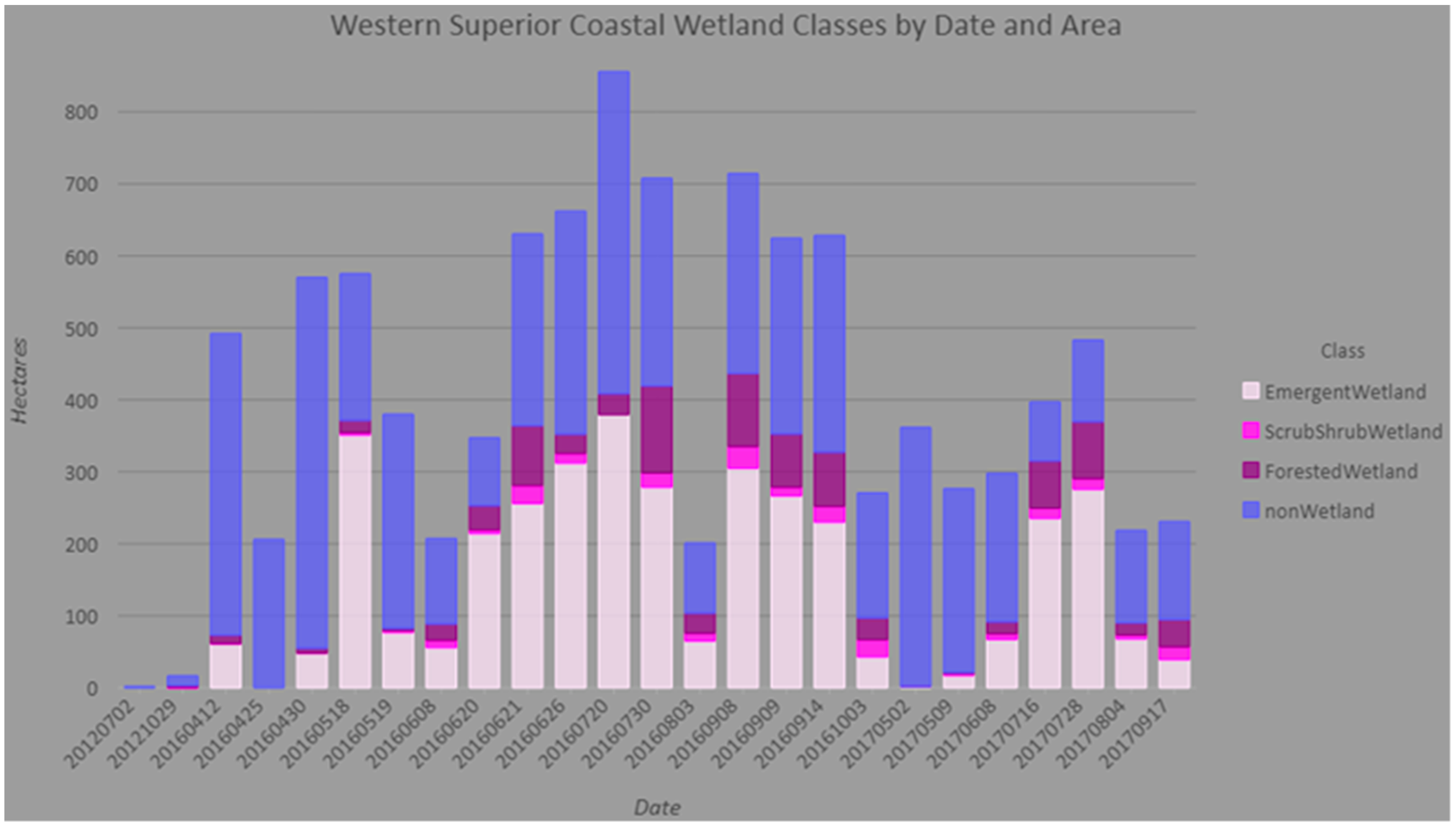
The Western Lake Superior region imagery was processed in batch and parallel using eCognition Developer (Trimble). These results were then manually reviewed and used to construct bar plots showing wetland area for the range of dates in the imagery archive and all of the wetland polygons (n = 192) in the Western Lake Superior region (Figure 10). The Western Lake Superior region had 188,430 unique wetland polygons that cover 13,928.6 ha. This wetland product was created to integrate an existing wetland product used by stakeholders with up-to-date, value-added information. The next phase of the project will extend the wetland mapping to the entire basin and all GLCWI polygons.

4.2.3. SAR Based Classification Approach

While the classification approaches above show that optical imagery can be used to aid in accurately classifying wetlands, cloud cover often prohibits their use during critical times throughout the growing season. In addition to its sensitivity to moisture and structure conditions of wetland vegetation, Synthetic Aperture Radar (SAR) has the ability to penetrate clouds and collect data regardless of sun-illumination conditions. However, models based on SAR data alone are sometimes not able to achieve acceptable wetland classification accuracies, though sometimes accuracies can be improved by including a Digital Elevation Model (DEM) and or Digital Surface Model (DSM) [29].
We tested RADARSAT-2 SAR data alone or in combination with a DEM/DSM to determine if it could be used to accurately classify the most common and spatially extensive wetland types throughout the Great Lakes basin. To do this, we constructed multiple Random Forest models with SAR data alone and in combination with a DEM/DSM and evaluated whether differences were statistically significant based on the McNemar’s Test [57]. Models were also constructed with single and multi-angle SAR data, as well as imagery from the spring, summer, or both to determine if multi-angle or multi-temporal data improved wetland classification. These models were all constructed with and without the DEM/DSM to determine whether these data improved accuracies. The aforementioned models were then re-run using simulated compact polarimetric (CP) RADARSAT Constellation Mission data (RCM) instead of RADARSAT-2. This allowed us to compare FP to CP data and to determine if the loss of polarimetric data in the CP mode, as well as the higher noise-equivalent sigma zero (NESZ) on RCM data, will affect the accuracy of wetland classifications.
To assess how multi-temporal data and acquisition timing affected classification accuracy, different models were constructed based on (1) spring (April/May), (2) summer (July), and (3) the combination of spring and summer data. Six land cover classes were included in the summer and spring and summer classifications: (i) water; (ii) shallow water; (iii) marsh; (iv) swamp; (v) agriculture/non-forested; and (vi) forest (Table 5). For all spring models, however, the shallow water class was not included due to a lack of vegetation at that time (i.e., these areas consisted only of open water).
Training and validation points were created by randomly distributing 500 points evenly throughout the entire study area. Afterward, each point was labelled as one of the six land cover classes based on a combination of field visits, and visual interpretation of UAV, WorldView, and Landsat imagery acquired between 2016–2018 in the spring, summer and fall. To sample each land cover class proportionally, additional training points were added by manually drawing polygons, randomly distributing points within them, and assigning each point an appropriate class label. 60% of these data were used as training data, while the remaining 40% were reserved for validation. Additional details on the training and validation methodology can be found in [57].
RADARSAT-2 imagery was acquired at both relatively steep (23.3–25.3° FQ5W beam mode) and shallow (36.4–38° FQ17W beam mode) incidence angles, twice throughout the growing season of 2016 (FQ5W: 1 May and 12 July, FQ17W: 27 April and 8 July) to assess how multi-angle data and acquisition timing affected classification accuracy. Previous research has shown steep incidence angles are better able to detect moisture and/or open water [58,59], whereas shallow incidence angles can more accurately map vegetation phenology, height and density [60]. The imagery was acquired to represent conditions before and after leaf-out to investigate optimal image timing to separate the classes considered here.
PCI Geomatica 2017 was used to process the RADARSAT-2 imagery, including calibration to sigma-naught, speckle filtering, and orthorectification. Variables included in the classification models were generated and stored in one multi-channel file (Table 6). Simulated RCM data was generated as described in Section 4.1.2. For this study, the simulated RCM data were not resampled to the nominal pixel spacing of the RCM beam modes. Instead, the same pixel spacing as the RADARSAT-2 data was used to avoid additional filtering (13.6 and 8.9 m for the FQ5W and FQ17W data). In instances where both beam modes were used in the model, the FQ17W was re-sampled to match pixel spacing of the FQ5W data.
The MNRF DEM and DSM data (Land Information Ontario) were created using 20 cm stereo orthophotos acquired between 2013 and 2015. Only the vertical accuracies of the DSM were reported, which differed by topography and land cover type. For example, the accuracies were ±15 m for open fields and ±6.36 m for deciduous trees at the 95% confidence level [61]. To remove noise over the water we applied the approach described in Behnamian et al. [40]. From these data, several derivatives were generated using the System for Automated Geoscientific Analyses (SAGA).
To classify all of the RADARSAT-2 and simulated RCM data we used the randomForests package in R [62,63]. For all models, 1000 trees were produced, and default settings were used to calculate the number of variables tested at each node and the final number of nodes to be created. Complete details and justification for these processing parameters can be found in [29,57,64].
Four different metrics were used to assess model accuracy: (i) independent overall accuracy (proportion of all validation points that were correctly classified), (ii) independent overall accuracy of wetlands (proportion of all validation points for wetlands that were correctly classified), (iii) user’s accuracy (for each class, the proportion of points classified correctly), and (iv) producer’s accuracy (for each class the proportion of points classified correctly divided by the number of validation points for that same class). To determine the statistical significance between the classification results, the McNemar’s test with a 95% confidence interval was applied [65]. For complete details on the data and methodology readers are referred to [57].
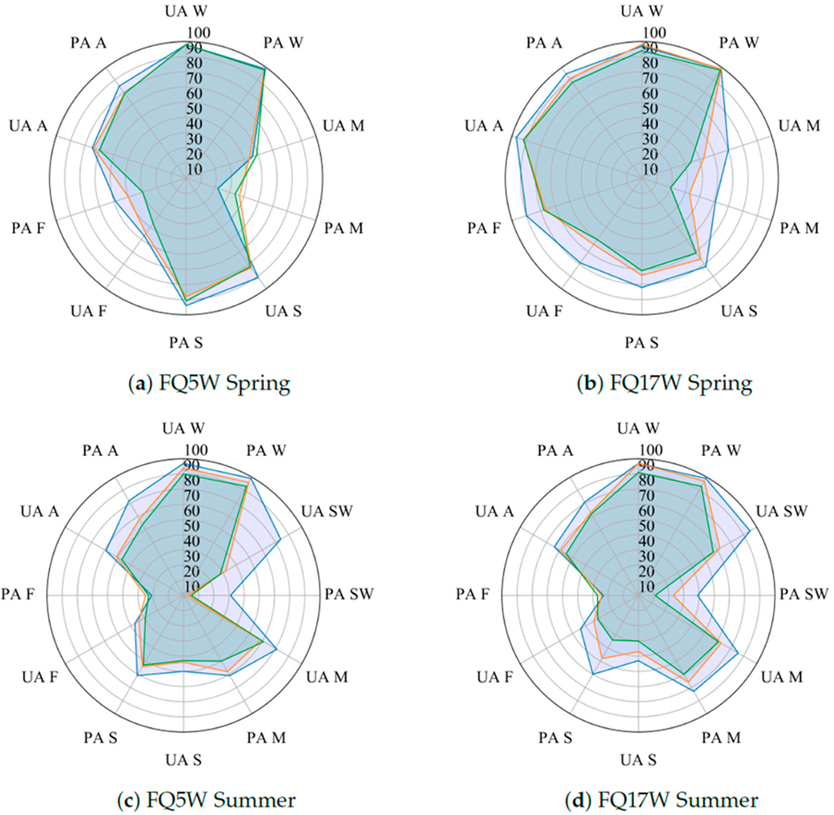
No Random Forest model based on a single SAR image was able to produce high accuracies (≥~80%) for all classes (Figure 11). The addition of high-resolution DEM and DSM data resulted in statistically significant improvements in model accuracy in all cases, however, only models based on the FQ5W spring and FQ17W spring images in combination with DEM and DSM data achieved per-class user’s and producer’s accuracies above 80%.
For models based on single SAR images, those constructed with the simulated RCM CP data achieved significantly lower accuracies than those constructed with RADARSAT-2 FP data, however, following the addition of DEM/DSM data, accuracies were more comparable between models based on simulated CP and FP data. This suggests that with CP data, more information from a variety of different sources, are required to obtain the same accuracies as those achieved with FP data. Additionally, medium resolution CP models generally had higher accuracies compared to high resolution CP models. These results were not surprising given the higher NESZ value of the high-resolution mode data.
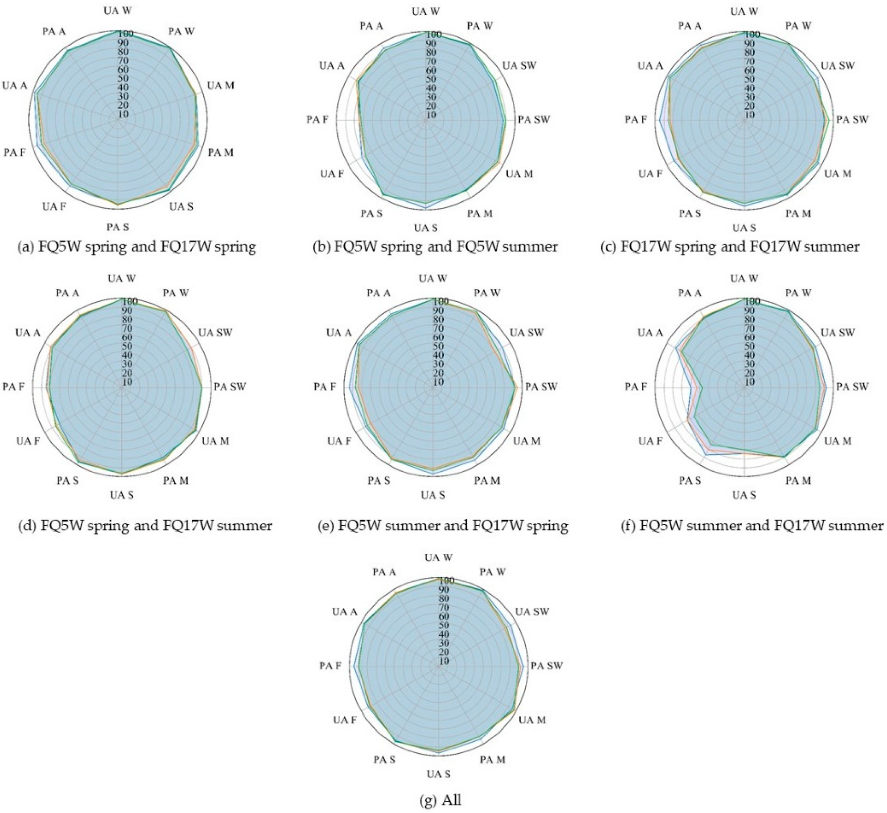
For models based on FP data, accuracies improved significantly when multi-temporal data (two or four images) were used as inputs to Random Forests. In fact, all models using multi-temporal (spring and summer) FP imagery achieved high accuracies (≥80%) for all classes, regardless of whether generated with data acquired at steep or shallow incidence angles (Figure 12). These findings are consistent with others that similarly concluded using multi-temporal SAR data improved wetland classification [22,64], and can be explained by the fact that similar backscatter characteristics were observed for multiple classes in either spring or summer, making them difficult to separate at those times. For example, the marsh and swamp classes had comparable proportions of double-bounce and volume scattering in the spring, however, those proportions differed in the summer (Figure 12). Consequently, by including both spring and summer RADARAT-2 imagery, separability between both classes improved. Similar results were observed for shallow water and agriculture/non-forested, which were more confused in the summer than in the spring.
Notably, for models based on multi-angle/multi-temporal data, the addition of the DEM/DSM only improved accuracies in some cases (overall accuracies improved by 1–21% for all models). For those based on simulated CP data, however, accuracies increased significantly in almost all cases, further demonstrating the importance of this additional information source for achieving comparable accuracies to the FP data. Exceptions included models based on two summer images and models based on all four CP images, for which accuracies were already high, and therefore a statistically significant difference was not observed following the addition of the DEM and DSM.
In most cases models based on medium resolution CP data had higher accuracies than those based on high-resolution CP data. However, this difference was on average less than 5% for all classes, except shallow water. This is as a result of the NESZ value of RCM data, in addition to fewer training and validation points, which caused additional confusion with agriculture/non-forest. Future RCM data users should consider the fact that both the medium and high-resolution beam modes have the same swath width, so one may be more advantageous than the other.
Results demonstrated that high classification accuracies could be achieved for the wetland classes in the Bay of Quinte with just multi-angle/temporal SAR data, and in some cases with just one SAR image, DEM and DSM data. For CP data, both multi-angle and multi-temporal data were needed to obtain acceptable classification accuracies for all classes. The addition of a DEM/DSM increased model accuracies significantly in all cases when only single SAR images were used, and in some cases with multi-angle/multi-temporal data. Results suggest that RCM data shows promise to classify wetlands with high accuracy. The high-revisit period of RCM will allow users to take advantage of multi-temporal and multi-angle data, both of which have been demonstrated as necessary to achieve high accuracies for all the classes evaluated here. These results will need to be verified with actual RCM data, especially since the NESZ values used to generate the simulated data were based on estimates.

4.2.4. SAR Based Change Detection Approach

In order to help prepare for the launch of RCM and determine its potential for mapping and monitoring wetland change we used simulated CP RCM data using the same simulation package described earlier in the medium resolution StripMap 16 m mode and compared it to FP RADARSAT-2 data in the Bay of Quinte, Ontario Canada. In this study, site there were three wetlands classes: (1) shallow water, (2) marsh, and (3) swamp. We applied the multi-temporal change detection method described in [24] to the FP RADARSAT-2 and the simulated CP RCM data. We then compared the sensitivity of each dataset to multi-temporal changes in wetlands and discussed how the amount of polarimetric information and NESZ values may have affected the results.
Single look complex (SLC), fully polarimetric (FP) RADARSAT-2 images from the spring and summer of 2016 were used in this study (3 April, 27 April, 14 June, 8 July, 25 August). All images were acquired in the FQ17W beam mode at 37.2° incidence angle in the ascending look direction. By using the same type of imagery, we were able to ensure that none of the changes we detected were from differences in the imaging geometry, but rather from changes vegetation, water level, or soil moisture. All wetlands in the study area were labelled as shallow water, marsh, or swamp. Descriptions of the classes are provided in Table 5. RADARSAT-2 and simulated RCM data were processed as described in Section 4.2.3.
Python code from [66] was used to apply a multi-temporal change detection method to all imagery. There were three main steps in the processing method: (1) estimate the Equivalent Number of Looks (ENL) for each coherency matrix, (2) co-register all of the matrices (stored as multi-channel files), and (3) detect the multi-temporal changes. There were also three raster outputs from the code, representing: (1) the timing of the first change, (2) the timing of the last change, and (3) the frequency of change.
Field data was not available to determine the cause of change. Instead, expert knowledge and mean intensity values, double-bounce, volume, and surface scattering contributions from the Freeman-Durden decomposition for 1000 randomly selected pixels for each wetland class were used to interpret the results. Note that because the same processing was applied to both the FP and CP data, we assumed that any differences in the changes detected between the two datasets were as a result of the differences in information content and NESZ values only. For more complete details about the data processing method readers are referred to [24].

Timing of First Change

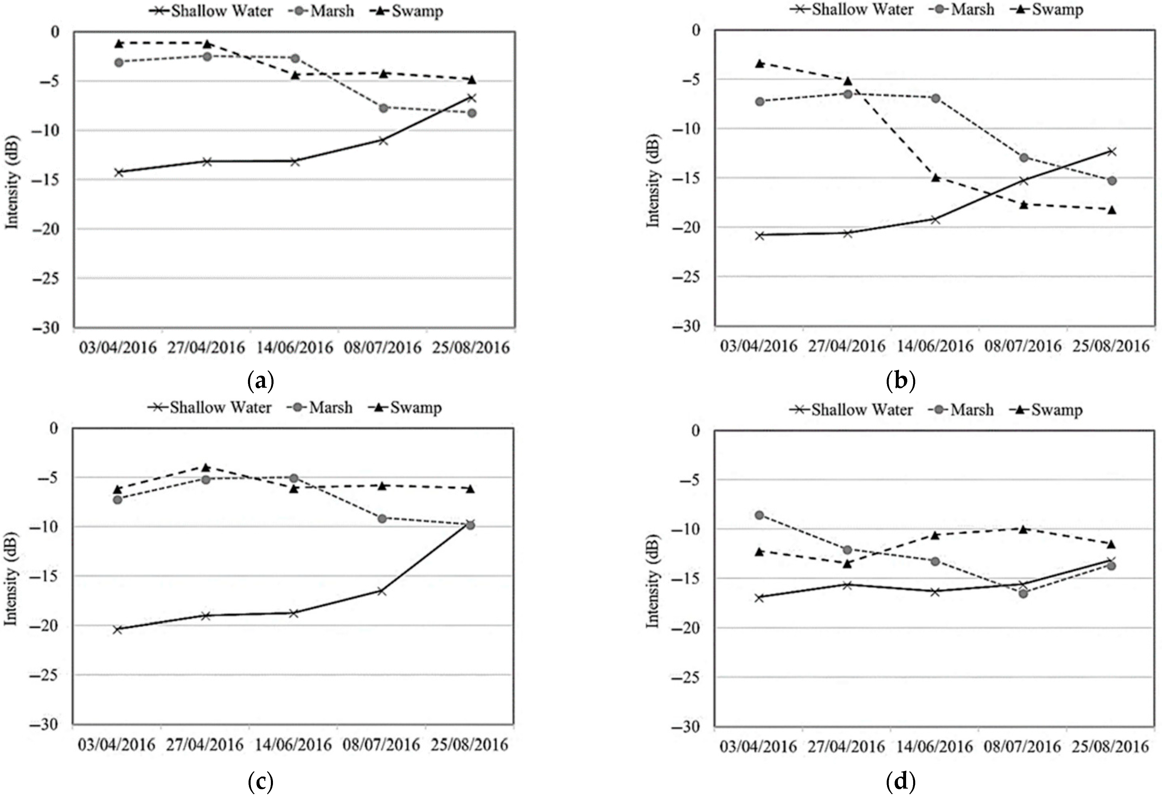
Both FP and CP data were able to detect changes within the wetlands throughout the growing season, but the timing and frequency of changes between the two differed (Figure 13). In some cases, the FP data was able to detect the first change in the growing season earlier than CP data (Figure 13a). For example, on 27 April the FP data recorded that 36 pixels in the shallow water class had changed in comparison to only 7 with the CP data. The same trend was observed for the marsh and swamp classes. On 27 April, change was detected for 253 pixels with the FP data for the marsh class, while change was only detected for 113 pixels with the CP data. On the same date, the FP data indicated that 148 pixels had changed in the swamp class, but the CP data only detected a change in 12 pixels (Figure 13a).
Capacity to detect change in the shallow water class was linked to several factors, including the combined effects of the size, shape, orientation, abundance and or spatial distribution of vegetation. Visual interpretation of WorldView data demonstrated that early season growth of lily pads, cattails and reeds (identified in some areas by June 6th) could not be detected in either the FP or CP data. It was theorized that this was due to the vegetation being relatively short in stature and low in density, resulting in predominant specular reflection and low backscatter returns, thus values were similar to the open water that was present beforehand (Figure 14). As the growing season progressed however, contributions of double-bounce scattering increased and the change from open water to vegetation was eventually detected in some cases by July 8th (Figure 14). July 8th was also the time when the first change was detected in a majority of cases for the marsh class. This is similarly attributed to growth to the increase in size and density of live cattails among a dense mat of senescent vegetation (mostly cattails). In contrast, the first change detected in a majority of cases for swamp was earlier in the season on June 14th. This change is attributable to the leaf out of the canopy, resulting in a significant decrease in the contribution of double bounce scattering (Figure 14). This occurred because of increased signal attenuation at the top of the canopy, preventing penetration to the flooded trunks below.

Timing of Last Change

In many cases, the FP data was able to detect changes at a later date compared to the CP data. For the shallow water class, change was detected for 865 pixels with the FP data on 25 August, but a last change was only detected for 784 pixels on this date with the CP data. The same was true for the marsh class, with change being detected for 463 pixels with the FP data on 25 August, compared to 254 with the CP data. In the case of the shallow water class, there was an increase in the intensity of the double-bounce backscatter from 8 July to 25 August, likely due to continued growth in the size and density of vegetation. For the marsh class, there was a large decrease in mean double-bounce values between July 8th and August 25th. This is likely due to increased attenuation within an increasingly dense vegetation canopy, thus resulting in volume scattering becoming the dominant contributor to total power (Figure 14). This decline in double-bounce scattering could also be due to lower water levels, which was confirmed with water level loggers in a few locations throughout the study area (e.g., decreases of of 2.47 and 1.98 m were observed at two different locations between 8 May to 8 July). This would have led to an increase in the path length between the signal and water level, leading to greater attenuation within the canopy.
Interestingly, for the swamp class, the first change detected on June 14th was also the last statistically significant change in the time series in a majority of cases, and this was observed with both the FP and the CP data (Figure 13). Results from the Freeman-Durden decomposition indicated that there was a large decrease in double-bounce backscattering (10 dB) from 27 April to 14 June (Figure 14). After this date double-bounce scattering had the lowest contribution to total power and volume scattering had the highest (Figure 14). This is again, likely due to the leafing out of the canopy preventing the radar signal from reaching the ground, resulting in an increase in volume scattering [67,68], though it is also possible that some swamps dried up throughout the growing season.

Frequency of Change

For all three wetland classes, the FP radar data detected a higher frequency of changes compared to the CP data. For the shallow water class, two changes were observed for the majority of pixels with both the FP and CP data. However, there were two changes detected in 668 pixels with the FP data and only 577 with the CP data. When we compared the number of pixels that had only changed once the CP data had 144 more compared to the FP data. For the marsh class, two changes were observed for most pixels (440) with the FP data, but only one change for most pixels (648) with the CP data. While both the FP and CP data only had one change for most of the pixels in the swamp class, 181 pixels for the CP data also had no change.

Differences between the FP and CP Data Change Detection Results

As noted earlier, FP RADARSAT-2 data provide complete target information, whereas CP data only provides only partial target information. This, together with the lower NESZ of the FP data, explains why the FP SAR being able to detect changes both earlier and later in the growing season, as well as a higher frequency of changes (Figure 10). However, when we quantitatively compared the change detection results between the FP and CP SAR data, there was greater than 90% agreement for all three wetland classes (Table 7). The shallow water class had the highest percentage agreement for the first change, last change, and frequency of change. The swamp class had the lowest percent agreement for the first (92.2%) and the last change (93.1%).
These results demonstrate the potential of RCM data to be used to detect changes in wetlands. Results indicated that the simulated RCM data was less sensitive to detecting the first change, last change and frequency of changes compared to RADARSAT-2 due to incomplete target information and a higher NESZ value. However, there was greater than 90% agreement for all three wetland classes included in this study. Future research is needed to validate these results using real RCM data.

4.3. Multi-Temporal Vegetation Elevation and Ecosystem Models

DigitalGlobe imagery, available under the NGA NextView license, is available in large quantities providing high temporal frequency and great levels of detail. The DigitalGlobe fleet includes the WorldView sensors which have the capability to collect stereo imagery. Stereo pairs image the same location from different angles, typically within seconds, enabling the development of high-resolution digital surface models (DSMs). The DSMs represent the elevation of the vegetation canopy, as opposed to the height of the ground represented by standard Digital Elevation Models (DEMs). The DSM products are useful individually when combined with accurate DEM information, providing insight into vegetation canopy height, which can be used to distinguish trees, shrubs, and emergent vegetation. When multiple DSMs are available for a single location, it is possible to assess changes in vegetation characteristics, allowing researchers and managers to explore the cause of the changes (e.g., development, water level changes, invasion by non-native plants).
A significant challenge when dealing with basin-wide high resolution stereo coverage is the ability to store and process the data. This task, handled by SharedGeo, required specific hardware and software infrastructure. Local computers, servers, and internet connections were installed at SharedGeo and the University of Minnesota to support data storage and transfer. Storage was upgraded to over 200 TB to accommodate imagery as it arrived.
The tool used for creating digital surface models from satellite imagery was SETSM photogrammetric software [69], which is known to work well in the supercomputing environment. We evaluated the differences between running SETSM at 2 m versus 50 cm and also comparing the output to Ames Stereo Pipeline (ASP) [70] for the same scenes. Observations showed that the 50 cm outputs perform better in terms of missing a fewer number of small tree clumps compared to the 2 m SETSM output. However, we chose to continue running SETSM at 2 m due to processing constraints and file size considerations with 50 cm output.
The process we used for working with SETSM and its output in the supercomputing environment was developed by the Polar Geospatial Center (PGC) at the University of Minnesota (U of MN) [71]. By using this process, we took advantage of their experience and our outputs would be compatible with those produced by PGC and others for other parts of the globe. PGC cooperated with this project by providing post-processing of the SETSM output. We met frequently with the Polar Geospatial Center at the U of MN to coordinate, share strategies and avoid duplication of work, especially during the last 6 months as we examined and evaluated outputs together and found ways to improve processes. For example, we found that 50 cm tests on Blue Waters showed that for full scenes SETSM is running out of memory; this appears solvable with code changes that we plan to explore further. SharedGeo staff also assisted PGC in improving the job scripts to be more robust and reduce the number of errors and wasted computer time.
The amount of computation required to produce the surface models needed for this project was massive. It takes roughly 12 h on average for SETSM to produce a 2 m DSM for a single stamp pair. As we had tens to hundreds of thousands of stamp pairs to process, we needed a massive amount computer time, certainly more than SharedGeo could assemble locally or in the cloud, and more than what was reasonable to run at the Minnesota Supercomputing Institute at the University of Minnesota. The project team was awarded a grant with the help of the Minnesota Department of Natural Resources of 540,000 node hours of computer time on the NSF funded Blue Waters petascale supercomputer through the Great Lakes Consortium for Petascale Computation [72,73]. The massive amount of data ingested required an additional 495,000 node hours after the first phase. By using various charge rate breaks such as running interruptible jobs and taking advantage of times when Blue Waters was underutilized, we were able to process 107,000 stamp pairs in 812,000 charged node hours on Blue Waters.
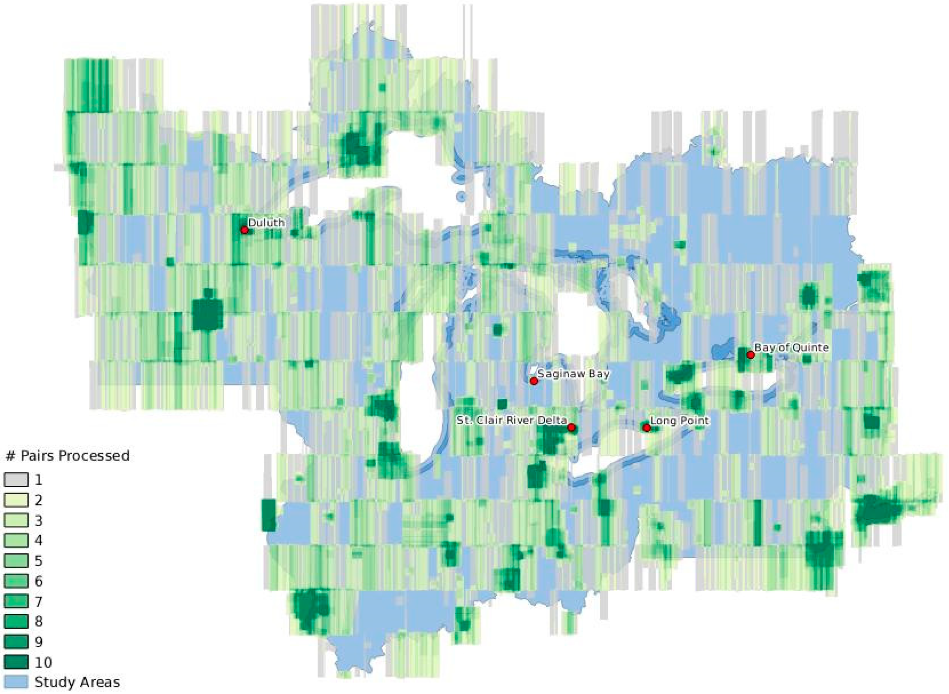
Imagery acquired from DigitalGlobe is indexed using “catalog IDs”. Two catalog IDs with spatial and temporal overlap can be used as a stereo pair which is the required input to produce a DSM. We obtained over 10,200 catalog IDs (5100 stereo pairs) from Digital Globe, covering 4,900,000 sq.km. in the primary study area in the Great Lakes Basin. In total, this includes over 13,000 stereo pairs covering over 14,400,000 sq.km. with acquisition dates primarily ranging from 2012–2018 with scattered coverage back to 2002 adding up to 100 TB of data (Figure 15).
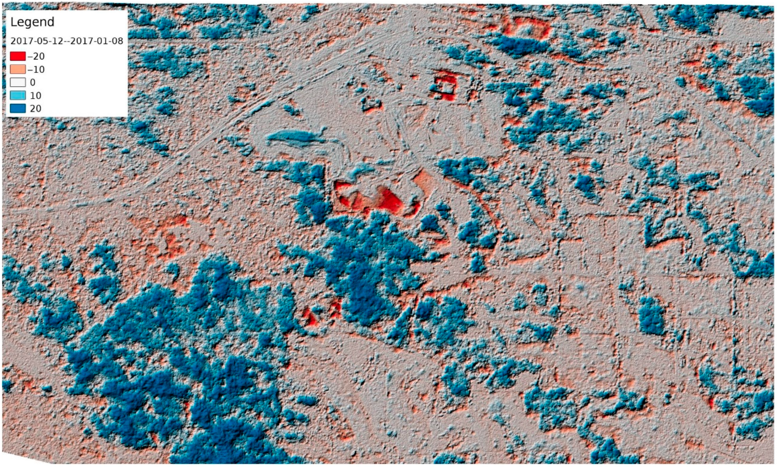
Each DigitalGlobe stereo pair is made up of roughly 8 stamp pairs. We produced over 107,000 of 2 m surface models (DSMs) from the DigitalGlobe stamp pairs. The PGC post-processing procedure combines the stamps back into strips and filters out unreliable areas in the data, such as areas obscured by clouds. PGC has continued to improve the filtering process and move it from Matlab licensed code to Python which may allow us to incorporate it into a workflow that is transportable to other systems that leverage open-source software. Analysis of multi-temporal DSM outputs has shown the utility of using them to detect changes in vegetation height and other anthropogenic changes. The example below shows changes between winter and late spring acquisition dates (Figure 16).
In the winter leaf-off scene the ground between the trees was visible and was the main feature detected for determining the elevation. In the late spring, the canopy (where present) obscured the ground from view as was detected as an increase in elevation. Figure 15 shows both the blue increase in elevation from the tree canopy change from leaf-off to leaf-on, but also anthropogenic change, determined to be mining activity, as the red area in the center.
Evaluation of various DSMs found the root mean square error (RMSE) is in the range of 1.2–1.6 m. This means any change detection is better suited to large vegetation disturbances and construction projects vs. smaller fluctuations such as water level changes. We also found that the DSMs measure different things based on time of year. In particular, leaf off vs. leaf on allows easy identification of deciduous forests, and provides the ability to measure ground elevation in the leaf off scenes.
To this point, all available sub-meter, commercial optical satellite imagery for the Great Lakes Basin have been processed and will continue to be processed to create surface vegetation elevation models to two-meter resolution. Continued acquisitions have been tasked to fill in the gaps and create summer and winter surface elevation models.

4.4. InSAR Water Level Monitoring

High interferometric coherence may be maintained in inundated wetlands with repeat-pass SAR observations due to the double-bounce scattering occurring between the water surface and vertically oriented vegetation, thus permitting the generation of InSAR interferograms and reliable measurements of phase variations related to water level changes [74]. Fluctuating water levels in dynamic water bodies, such as the Great Lakes affect SAR backscattering coefficients, InSAR coherence and interferograms over marshes [74]. Given the high coherence and double-bounce scattering as main scattering mechanism in the wetland, we theorize that the deformation is the result of water level changes. It is important to understand the potential to use InSAR to monitor water level fluctuations in various wetland environments in the Great Lakes Basin. Although all polarizations can be used to generate interferograms, previous studies [75] have shown that coherence values are the highest for HH, followed by VV, and HV or VH being the lowest. Coherence in wetlands is generally lower in acquisitions over two repeat cycles than that of one repeat cycle for Radarsat-2 C-band data (24 days for one repeat cycle) [74]. As such, the small baseline subset (SBAS) technique [76] may be exploited to use all the interferograms with short temporal and spatial baselines for wetland water level studies [74,75]. To address the objective of using InSAR to monitor wetland water level change in the Great Lakes Basin, C-band SAR data of HH polarization from Radarsat-2 are investigated using the SBAS based method to evaluate the suitability of InSAR in different wetland environments, including shallow water, marsh and swamp in two study areas, Bay of Quinte, Ontario, and Long Point, Ontario Canada.
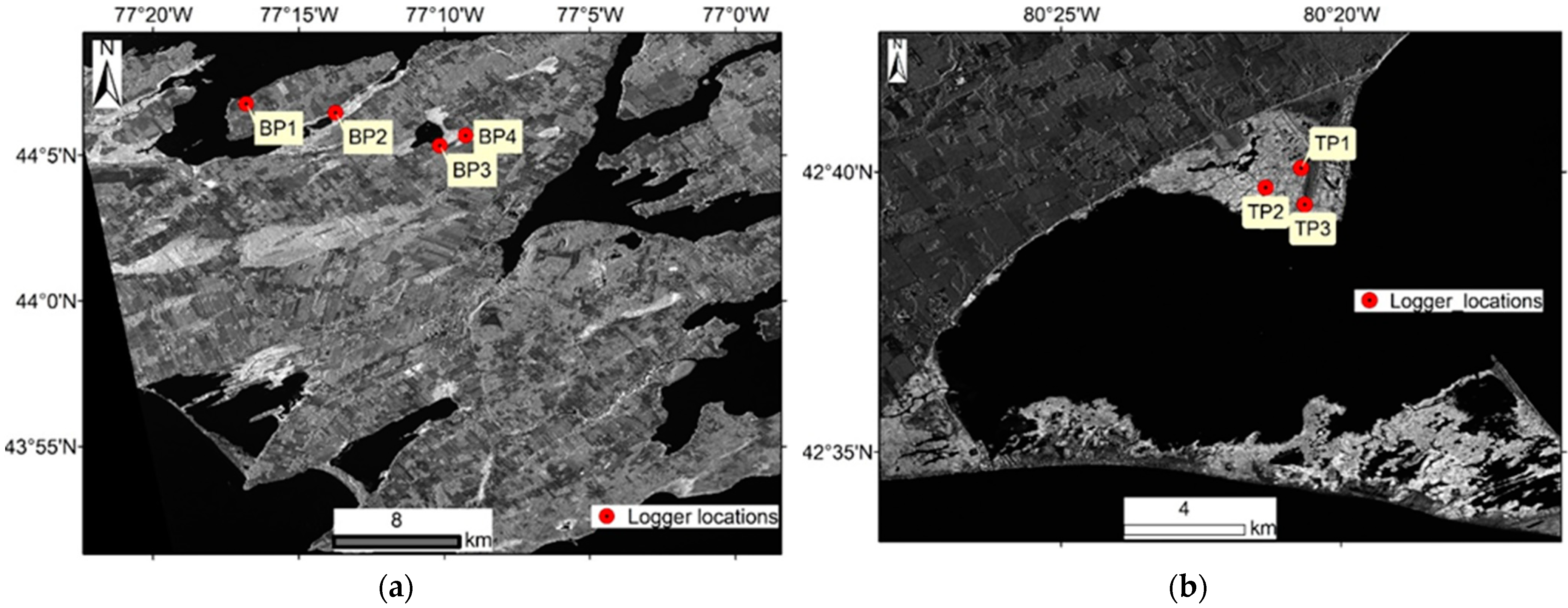
For the Bay of Quinte study area (Figure 17a), readers are referred to the description of the Bay of Quinte above. Nine scenes of Radarsat-2 FQ5W mode, eight scenes of Radarsat-2 FQ17W, seven scenes of Radarsat-2 U7W2 mode were collected. The FQ5W and FQ17W datasets were quad polarized (HH, HV, VV, VH) while the U7W2 data was single polarized (HH).
The Long Point study area is located on the Canadian side of Lake Erie in Ontario (Figure 17b), and encompasses Turkey Point (TP), the National Wildlife Area at Big Creek (BC), the Long Point Provincial Park and Crown Marsh at Old Cut (OC), and the National Wildlife Area at Thoroughfare (TH). Both shallow water and marsh wetland types were considered in this site. Marsh is the dominant wetland type in Long Point, characterized by an interspersion of marsh meadow and emergent aquatic vegetation, primarily dominated by cattail and/or common reed (Phragmites australis). Both cattail and Phragmites are normally 2–3 m tall and are capable of forming dense stands. Seven scenes of Radarsat-2 FQ1W mode, eight scenes of Radarsat-2 FQ18W, eight scenes of Radarsat-2 U23W2 mode were collected. The FQ1W and FQ18W datasets were quad polarized (HH, HV, VV, VH) while the U23W2 data was single polarized (HH). Only the data of HH polarization from Radarsat-2 acquired within 24 days was evaluated.
Solinst water level loggers were installed in two locations in the marsh and two locations in the swamp in Bay of Quinte (Figure 17a), and three locations in the marsh in Long Point (Figure 17b). Water level measurements from loggers were collected from April to November in 2018 to validate InSAR measurements. In Long Point, the water levels over three locations near Turkey Point also provided information for investigating the sensitivity of InSAR measurements to changes in the elevation and direction of flow of water for transects running from south to north and from southwest to northeast.
Traditional differential InSAR (D-InSAR) processing was applied first to produce D-InSAR measurements. This procedure included co-registering and resampling all the InSAR images from one orbit (same polarization and incidence angle) to the same reference image, generating differential interferograms, and phase unwrapping using the Minimum Cost Flow algorithm [77] with a reference point. All InSAR processing was performed using GAMMA software. Multi-looking and resampling were applied to make all products of U7W2 at 10 m, FQ5W and FQ17W at 30 m for Bay of Quinte study area, and U23W2 at 10 m, FQ1W and FQ18W at 30 m for Long Point study area. Then coherence analysis was conducted to evaluate the quality of interferograms over different wetland types, and the influence of various incidence angles and resolutions on the coherence. Finally, water level change was extracted using SBAS methods.
In the coherence analysis, average coherence values were calculated for different wetland types. In Bay of Quinte, the coherence was calculated over the polygons containing shallow water (labeled as “Water”), and marsh vegetation composed primarily of cattail (labeled as “Cattail”), and swamp vegetation composed primarily of woody plants (labeled as “Swamp”). In Long Point, the coherence was calculated over the shallow water (labeled as “Water”), and marsh vegetation composed of a mix of cattail and Phragmites (labeled as “Cattail/Phragmites”), and marsh meadow dominated by grasses (labeled as “Grass”).
In the water level analysis, a coherence threshold of 0.3 was used to identify coherent pixels in each coherence map, then the SBAS approach was applied to measure water level changes observed in time series interferograms. In the SBAS analysis, the quality interferograms from the same mode were used to form a network of subsets containing the interferograms of small baselines, then the water level changes evolving over the time were extracted using the singular value decomposition (SVD) algorithm. Cumulative water level calculated from the SBAS analysis only provided relevant information for those pixels with high coherence and was then validated using in-situ measurements. A linear regression was applied to model their relationship. R square and root mean square errors (RMSE) were calculated to determine the significance of results.
Results for all four Radarsat-2 modes indicated that Cattail has higher coherence values than Swamp and Water in Bay of Quinte. For example, average coherence values were 0.55–0.69 for Cattail, 0.39–0.54 for Swamp, and 0.32–0.43 for Water (Table 8). Results showed that coherence values varied in different swamp areas throughout the season. For example, sparser canopies observed during April-May allows more penetration than the denser canopies observed between June-October. Overall, both backscattering power and coherence over swamp were higher in the early season than the later season.
Results in Long Point demonstrated that coherence from Cattail/Phragmites was generally higher than that from Grass and Water in all three modes. For example, coherence values were 0.72–0.77 for Cattail/Phragmites, 0.41–0.62 for grass, and 0.21–0.28 for shallow water (Table 9).
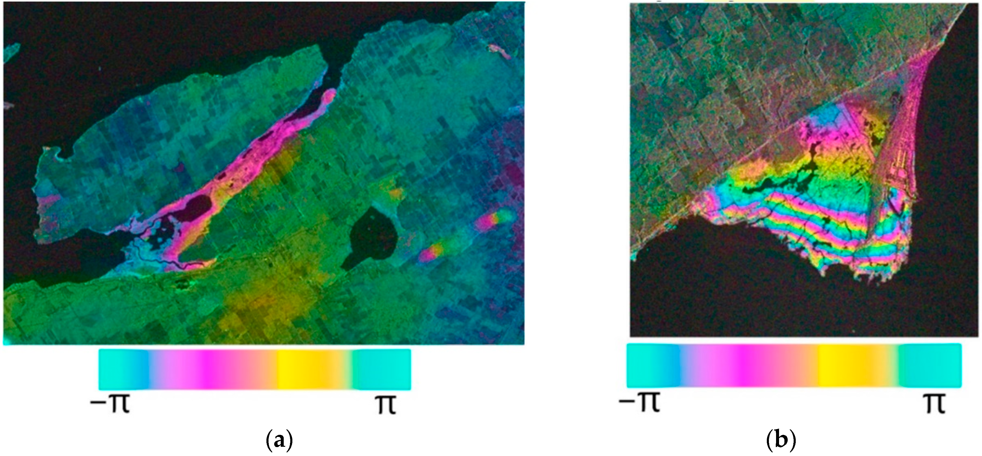
The results from the coherence analysis in both areas indicated that coherence in marsh dominated by Cattail or Cattail/Phragmites remained the highest, followed by Grass, then Swamp. Water had the lowest coherence. It seems that change in incidence angles and resolution did not affect coherence in Cattail or Cattail/Phragmites dominated marsh, although the small size of wetlands in the Bay of Quinte may not be accurately represented by coarse resolution. When the wetland size was less than 100 m by 100 m, the averaging process for coherence calculation might include the neighborhood of non-wetlands. It was found that the changes of interferogram fringes mainly occurred in wetlands, which indicated water level changes (Figure 18).
InSAR results in Bay of Quinte were validated at four locations using field measurements in 2018. Both positive and negative correlations between field measurements and InSAR observations were found in BP1 and BP2 locations from the cattail dominated marshes, and BP3 and BP4 locations from the swamps (Table 10). For all three imaging modes there was a strong positive correlation with field measurements at both BP2 (a marsh site) and BP3 (a swamp site). However, there were mixed results in the other two sites. In particular, low correlation was found in BP4 (a swamp site) from FQ5W and FQ17W modes (correlation of 0 and −0.1 respectively). RMSE values of up to 38 cm were also observed when comparing InSAR to field measurements. Therefore, it was not possible to draw conclusions on the effect of incidence angle and resolution. Results indicated that the finer resolution mode U7W2 performed better than other modes in swamp with a positive correlation and smaller RMSE values, and FQ5W performed better in marsh compared to U7W2 and FQ17W.
InSAR results in Long Point were validated at three locations using field measurements in 2018. Only results from FQ18W were positively correlated with field measurements of water level changes in all three marsh locations (Table 11). Results generated from the other two datasets were variable in three locations, although the finer resolution U23W2 had smaller RMSE values.
Differences in water level along the southwest-northeast transect (TP2_TP1, Figure 17) and the south-north transect (TP3_TP1) detected using InSAR were compared with that measured by in-situ instruments. Results indicated that the InSAR measurements from all three modes were sensitive to the water level change along the southwest-northeast transect, but uncertainty remained along the south-north transect (Table 12). Note that there was little water level difference in the east-west direction in the study area and so results for that transect were inconclusive. Overall, the finer resolution U23W2 was observed to be more sensitive than other modes in measuring the change along the flow path.
Based on the results from coherence and water level analyses, it was not possible to draw conclusions on the effect of incidence angle, and resolution on InSAR measurements. We found that generally, InSAR interferograms from finer resolution images produced clearer fringe patterns than those from coarser resolution images in both study areas. Finer resolution data may more adequately represent changes in smaller wetlands. In-situ measurements in both the Bay of Quinte and Long Point showed that daily water levels fluctuated by up to 30 cm, with the greatest variations being observed in April, and between September and October 2018. Marshes had more water level variations than swamps, however, the coherence of cattail/Phragmites dominated marshes was higher than in swamps.
The correlation analysis produced mixed results for the different locations and imaging modes, with variable correlation values and large RMSE between field-measured water level and InSAR measurements. This is largely as a result of the combination of high fluctuations in water levels that occurred over short time periods, and the relatively long-time interval between SAR observations. Higher RMSE values between InSAR and in-situ field measurements in the marsh in Bay of Quinte (compared to that of Long Point) was due to low variation of the interferogram fringe. The low coherence in swamp also resulted in low correlation between field measurements and InSAR observations in FQ5W and FQ17W modes in one of the swamp areas. Only half a fringe was measured throughout most interferograms for the Bay of Quinte, compared to 1–2 fringes in Long Point. Therefore, a large RMSE was found between InSAR and field measurements. For example, although a correlation of 0.87 was found with FQ5W observations, the RMSE represented up to a 38 cm offset between InSAR and field measurements. Given fewer observed fringe cycles, and the large RMSE between InSAR observations and field measurements in this study, C-band data with a 24-day repeating cycle may not be sufficient to detect water level changes in areas like the Bay of Quinte and Long Point, where there is dynamic water level change (both daily water level and accumulated water level > 10 cm).
Overall, these results demonstrated that InSAR phase changes were sensitive to differences in water level and in the direction of flow in some cases. Although observed coherence in marshes was generally high, results from correlation and RMSE analysis showed that the relationship between InSAR measurements and field-based water level changes varied depending on the site, type of vegetation, and incidence angle. Resolution and incidence angles did not affect the coherence quality in large wetlands. Results suggest that InSAR observations based on C-band data, within a 24-day repeat cycle, may not be sufficient to maintain temporal coherence, and thus to also represent the water level changes in such dynamic wetland environments. Further studies on the potential of InSAR for water level monitoring with long term observations in various study sites and SAR sensors with shorter repeat cycles will be considered. Given a shorter acquisition cycle of four days with a constellation of three satellites, the RCM data is expected to improve InSAR applications because higher coherence can be maintained within a shorter time period, which may make it possible to detect dynamic water level changes in the future.

5. Discussion

While at various stages of development, the results here demonstrate capabilities for accurate dynamic mapping and monitoring of Great Lakes coastal wetlands at various study sites around the region. Surface water detection methods derived from multi-temporal RADARSAT-2 and simulated RCM data are demonstrated as suitable for monitoring seasonal, annual, and interannual hydroperiod. Errors in the operational implementation of these approaches can be reduced with ancillary impervious surface data layers, thus differentiating water from other flat surfaces such as parking lots and regions of bare soil, such as cropland. The use of SAR sensors for this application has advantages over methods utilizing optical sensors [78,79,80] in that they are not obscured by clouds or other meteorological conditions and the ability to penetrate vegetation canopy allows for direct assessment of flooded vegetation extent rather than inference based on previous surface water extent or modelling. However, the ability to detect subcanopy flooding with C-band SAR in higher biomass cover types, such as shrubby and treed swamps, is variable and dependent on a variety of conditions such as canopy structure, incidence angle, and stem density [81,82,83]. While incidence angle is consistent for our study areas, locations where vegetation structure or density precludes flood detection is not well characterized in our study areas yet. This capability is likely dynamic as leaf area increases significantly early in the growing season. Additionally, high density emergent vegetation such as Phragmites australis also appears to be too dense to penetrate at C-band in some cases, but the threshold at which flood detection is no longer possible is not known, which is may result in significant omission error. Additional work, including collection of additional field data to parameterize algorithms specifically to different vegetation types and to determine the applicability of the methods described herein to actual RCM data is needed to improve monitoring capability of C-band. The utility of L-band SAR, which has shown to be superior to C-band for detection of flooded forests [81], will be greatly increased with the launch of NISAR in 2022. In addition to the increased penetration of L-band, NISAR will also provide improved temporal resolution with a repeat cycle of 12 days, allowing for a more accurate understanding of surface water extent dynamics.
The multiple wetland classification approaches presented each provide strengths and weaknesses but are all effective at mapping wetland type at high resolution with reasonable accuracies. Each of these methods may be preferable under different circumstances depending on the needs of the end user. For invasive species monitoring, the SAR-multispectral approach may be ideal, however, for assessments of seasonal wetland variability the SAR/DEM approach is likely preferable. While the approach combining multi-temporal SAR and multispectral data is preferable for mapping to the species level, the reliance on multi-temporal data diminishes the ability to detect short-term changes. It also presents major challenges in terms of automation as it requires large amounts of supervised training data and human analyst intervention. The huge volumes of data available via cloud-computing platforms has begun to make multi-sensor classification approaches applicable to vast regions [84], though there remain limitations including lower spatial resolution and limited sensor availability.
Multi-temporal SAR combined with DEM/DSM data shows very promising results with high accuracies achieved in the pilot study areas and presents a feasible solution for cloud-obscured regions where clear multispectral image collections are rare, especially with the high repeat cycle that will be available via RCM. Simulated RCM data was also able to adequately assess short term temporal changes within wetlands. The addition of L-band data will likely increase classification accuracy, as multi-frequency SAR has been shown to have good results for wetland classification in the Great Lakes [85], and multi-frequency classifications have slightly higher overall accuracies compared to single-frequency classifications [86]. Therefore, the potential of combined RCM and NISAR data could prove to be unparalleled for dynamic wetland monitoring.
The OBIA approach, while lacking some detail in terms of class distinctions, presents a reasonable method for assessments of wetland gain and loss and presents a high likelihood for automation due to the simple rule-set based approach. Some researchers have argued that OBIA approaches result in higher accuracy classifications [87] and they also have the advantage of being easier to interpret to those who are not remote sensing experts [88]. These advantages could be exploited further with incorporation of SAR data, or derivatives of the SAR data, into the OBIA processing chain. Integration of SAR data with high-resolution imagery and vegetation height change metrics derived from DSMs in the OBIA framework could provide wetland change products with high enough temporal resolution to aid in both policy decisions as well as wetland management decisions. Further research is needed to assess how to best incorporate all of these data sources.
Remote assessment of water-level change within wetlands is possible under some conditions using InSAR techniques, but the 24-day repeat cycle of RADARSAT-2 is often too long to ensure high coherence between subsequent images. While Sentinel-1 has a higher repeat cycle, its standard collection mode over the Great Lakes acquires VV and VH data, which produces lower coherence values in common Great Lakes vegetation types [74]. The more frequent repeat cycle of RCM will likely improve this capability, especially under high resolution collection modes. The availability of L-band sensor data, such as the planned NISAR satellite, will also likely improve InSAR derived water level change measurements as the lower frequency radar energy will be more likely to penetrate dense marsh and swamp vegetation. InSAR with L-band sensors has been used to assess water level change in other regions with dense wetland vegetation such as the Everglades [89], the Great Dismal Swamp [90], and the Amazon [91]. The ambiguity of phase-unwrapping at C-band with water level changes should not be an issue with the longer wavelength of L-band.

6. Conclusions

The Great Lakes represent ~20% of the planet’s available surface freshwater. As demonstrated in geologic time, the polar ice caps and Greenland will eventually melt into the ocean removing a significant surface freshwater source. In that scenario, the aforementioned 20% rises to nearly 50% assuming the Great Lakes do not change. With the increasing effects of climate change, it is imperative to increase our Great Lakes Basin remote sensing programs for dynamic monitoring of our coastal and inland freshwater lakes and wetland systems, which help maintain the overall health of the Great Lakes as a whole. The results shown here represent the first steps towards this goal.
Future work following on from the efforts presented in this paper will include product integration and further progress towards product automation. One of the activities in the next phase of this project involves expanding the wetland classification and monitoring activities to all of the DigitalGlobe/MAXAR imagery available for the Great Lakes basin. This will also require ingestion of RCM data as it becomes available as it is not anticipated that RADARSAT-2 acquisitions will increase in frequency and it is beyond its life expectancy. The application of methods described here to the entire basin will require a fully automated classification workflow. This approach is being developed using free and open-source geospatial software in a super computing environment. Open software tools provide the opportunity to create robust, custom solutions with transparency that is often missing from commercial software. The tools and workflows can then be distributed to decision managers and researchers interested in applying this approach to other regions. In addition to creating open tools, output products will be distributed and available to end-users.
As remote sensing-based technology and methodology continue to advance and spatial, temporal, and radiometric resolutions of available sensors increase, our ability to monitor Great Lakes wetlands will only continue to improve. Wider availability of low frequency SAR from RCM, NISAR, and other planned missions will improve our ability to detect small changes in water elevation and extent, while high resolution multispectral satellite imagery will provide more detailed information on vegetation height, species composition, and invasive species spread. The ability to fully automate these approaches will also be important as data volumes increase and it becomes imperative to harness available and emerging technologies, such as supercomputers, cloud-computing, and machine-learning techniques.
As these capabilities improve, the authors stress the importance of regular communication with land managers, policy makers, and other stakeholders to ensure that remote sensing derived products are created with end user applications in mind. While each product has its own potential use-cases, coordination with end users will guide ways to effectively fuse products described above for widespread utility amongst the wetland science, management, and policy community. As follow-on, a second survey of wetland managers was recently released along with an ESRI storymap depicting some of the products. In addition, the researchers have presented and requested feedback at a myriad of wetland and Great Lakes conferences and workshops, as well as to the Great Lakes Coastal Assembly, IJC, Lake Superior Collaborative, and more. Future outreach plans include building a website with product information and recorded presentations on the various products, hosting a webinar series on coastal wetland monitoring, expanding the information in the ESRI storymap and continued conference and workshop presentations.

Author Contributions

Conceptualization, B.B., L.B.-C., B.H., J.K. (Joseph Knight); methodology, L.B.-C., A.B., B.B., J.K. (James Klassen), K.P., L.W., S.B., Z.C.; software, M.J.B., A.B., J.K. (James Klassen), K.P., P.M.; validation, M.J.B., S.B., A.B., Z.C., J.K. (James Klassen), K.M., K.P., L.W.; formal analysis, M.J.B., S.B., A.B., Z.C., J.K. (James Klassen), K.M., K.P., L.W.; resources, J.C.; data curation, J.K. (James Klassen); writing—original draft preparation, M.J.B., S.B., A.B., Z.C., L.W., J.K. (James Klassen), K.P.; writing—review and editing, All; visualization, M.J.B., A.B., Z.C., J.K. (James Klassen), K.P., L.W.; supervision, B.B., L.B.-C., B.H., J.K. (Joseph Knight); project administration, B.B., L.B.-C., B.H., J.K. (Joseph Knight); funding acquisition, B.B., L.B.-C., J.K. (Joseph Knight). All authors have read and agreed to the published version of the manuscript.

Funding

Michigan Technological University, University of Minnesota, and SharedGeo were funded by the U.S. Department of Interior, U.S. Fish and Wildlife Service with funding from the Great Lakes Restoration Initiative. Other contributors received no external funding.

Data Availability Statement

Restrictions apply to the availability of these data. Data was obtained from MDA Corporation through the NorthernView agreement and from MAXAR Technologies via the NextView License.

Acknowledgments

This large, binational project requires acknowledgement of many other unseen contributors: Robert Krska, U.S. Fish & Wildlife for instigating this project; Kevin O’Donnell, EPA for supporting the project, Colin Brooks, Michigan Tech Research Institute for mapping into the water without losing a UAS; Bob Ryerson, Kim Geomatics for his assessment of Great Lakes remote sensing research; Robb Macleod, Ducks Unlimited for stakeholder input; Steve Kloiber, MNDNR for updating the Minnesota NWI; Dan Heines, University of Minnesota for the Lake Superior UAS imagery, and the entire crews at SharedGeo and the Polar Geospatial Center for exposing the collaboration to petalscale computing. Finally, we also need to acknowledge the loss of Chuck Olson, whose research was instrumental in helping us observe the Great Lakes from near and far.

Conflicts of Interest

The authors declare no conflict of interest.

References

  1. Maynard, L.; Wilcox, D.A. Coastal Wetlands. State of the Lakes Ecosystem Conference Background Paper. 1997. Environment Canada and United States EPA. EPA 905-R-97-015b. Available online: https://greatlakesresilience.org/sites/default/files/library_reference_1997_SOLEC_CoastalWetlandsoftheGreatLakes.pdf (accessed on 18 January 2021).
  2. Albert, D.A.; Wilcox, D.A.; Ingram, J.W.; Thompson, T.A. Hydrogeomorphic classification for Great Lakes coastal wetlands. J. Great Lakes Res. 2005, 31, 129–146. [Google Scholar] [CrossRef]
  3. Krieger, K.A. The Ecology of Invertebrates in Great Lakes Coastal Wetlands: Current Knowledge and Research Needs. J. Great Lakes Res. 1992, 18, 634–650. [Google Scholar] [CrossRef]
  4. Dahl, T.E. Wetlands: Losses in the United States, 1st ed.; U.S. Fish and Wildlife Service: St. Petersburg, FL, USA, 1990; p. 13. [Google Scholar]
  5. Great Lakes Restoration Initiative. Great Lakes Restoration Initiative Action Plan III. 2019. Available online: https://www.epa.gov/sites/production/files/2019-10/documents/glri-action-plan-3-201910-30pp.pdf (accessed on 18 April 2020).
  6. Great Lakes Protection Initiative. 2018. Available online: https://www.canada.ca/en/environment-climate-change/services/greatlakes-protection/funding/2018-2019.html (accessed on 18 April 2020).
  7. Great Lakes Water Quality Protocol of 2012 (GLWQA). Available online: https://binational.net/glwqa-aqegl/ (accessed on 18 April 2020).
  8. Ingram, J.; Holmes, K.; Grabas, G.; Watton, P.; Potter, B.; Gomer, T.; Stow, N. Development of a Coastal Wetlands Database for the Great Lakes Canadian Shoreline; Wetlands2-EPA-03 Final Report to the Great Lakes Commission; United States Environmental Protection Agency: Ann Arbor, MI, USA, 2004; p. 18. [Google Scholar]
  9. Gronewold, A.D.; Rood, R.B. Recent water level changes across Earth’s largest lake system and implications for future variability. J. Great Lakes Res. 2019, 45, 1–3. [Google Scholar] [CrossRef]
  10. Gronewold, A.D.; Fortin, V.; Lofgren, B.; Clites, A.; Stow, C.A.; Quinn, F. Coasts, water levels, and climate change: A Great Lakes perspective. Clim. Chang. 2013, 120, 697–711. [Google Scholar] [CrossRef]
  11. Currie, W.S.; Goldberg, D.E.; Martina, J.; Wildova, R.; Farrer, E.; Elgersma, K.J. Emergence of nutrient-cycling feedbacks related to plant size and invasion success in a wetland community- ecosystem model. Ecol. Model 2014, 282, 69–82. [Google Scholar] [CrossRef]
  12. Cowardin, L.M.; Golet, F.C. US Fish and Wildlife Service 1979 wetland classification: A review. Vegetation 1995, 118, 139–152. [Google Scholar] [CrossRef] [Green Version]
  13. Fournier, R.A.; Grenier, M.; Lavoie, A.; Hélie, R. Towards a strategy to implement the Canadian Wetland Inventory using satellite remote sensing. Can. J. Remote Sens. 2007, 33 (Suppl. S1), S1–S16. [Google Scholar] [CrossRef]
  14. National Oceanic and Atmospheric Administration, Office for Coastal Management. Coastal Change Analysis Program (C-CAP) Regional Land Cover; NOAA Office for Coastal Management: Charleston, SC, USA. Available online: www.coast.noaa.gov/htdata/raster1/landcover/bulkdownload/30m_lc/ (accessed on 19 April 2020).
  15. Bourgeau-Chavez, L.; Endres, S.; Battaglia, M.; Miller, M.E.; Banda, E.; Laubach, Z.; Higman, P.; Chow-Fraser, P.; Marcaccio, J. Development of a bi-national Great Lakes coastal wetland and land use map using three-season PALSAR and Landsat imagery. Remote Sens. 2015, 7, 8655–8682. [Google Scholar] [CrossRef] [Green Version]
  16. Bourgeau-Chavez, L.L.; Kowalski, K.P.; Battaglia, M.J.; Poley, A.F. Land cover map including wetlands and invasive Phragmites circa 2017. U.S. Geol. Surv. Data Release 2019. [Google Scholar] [CrossRef]
  17. White, L.; Ryerson, R.A.; Pasher, J.; Duffe, J. State of Science Assessment of Remote Sensing of Great Lakes Coastal Wetlands: Responding to an Operational Requirement. Remote Sens. 2020, 12, 3024. [Google Scholar] [CrossRef]
  18. Ozesmi, S.L.; Bauer, M.E. Satellite remote sensing of wetlands. Wetl. Ecol. Manag. 2002, 10, 381–402. [Google Scholar] [CrossRef]
  19. Chan, Y.K.; Koo, V.C. An introduction to synthetic aperture radar (SAR). Prog. Electromagn. Res. B 2008, 2, 27–60. [Google Scholar] [CrossRef] [Green Version]
  20. Dabboor, M.; White, L.; Brisco, B.; Charbonneau, F. Change detection with compact polarimetric SAR for monitoring wetlands. Can. J. Remote Sens. 2015, 41, 408–417. [Google Scholar] [CrossRef]
  21. White, L.; Brisco, B.; Dabboor, M.; Schmitt, A.; Pratt, A. A collection of SAR methodologies for monitoring wetlands. Remote Sens. 2015, 7, 7615–7645. [Google Scholar] [CrossRef] [Green Version]
  22. Mahdavi, S.; Salehi, B.; Amani, M.; Granger, J.E.; Brisco, B.; Huang, W.; Hanson, A. Object-based classification of wetlands in Newfoundland and Labrador using multi-temporal PolSAR data. Can. J. Remote Sens. 2017, 43, 432–450. [Google Scholar] [CrossRef]
  23. Dechka, J.A.; Franklin, S.E.; Watmough, M.D.; Bennett, R.P.; Ingstrup, D.W. Classification of wetland habitat and vegetation communities using multi-temporal IKONOS imagery in southern Saskatchewan. Can. J. Remote Sens. 2002, 28, 679–685. [Google Scholar] [CrossRef]
  24. Dabboor, M.; Banks, S.; White, L.; Brisco, B.; Behnamian, A.; Chen, Z.; Murnaghan, M. Comparison of Compact and Fully Polarimetric SAR for Multitemporal Wetland Monitoring. IEEE J. Sel. Top. Appl. Earth Obs. Remote Sens. 2019, 12, 1417–1430. [Google Scholar] [CrossRef]
  25. Mahdianpari, M.; Granger, J.E.; Mohammadimanesh, F.; Salehi, B.; Brisco, B.; Homayouni, S.; Gill, E.; Huberty, B.; Lang, M. Meta-Analysis of Wetland Classification Using Remote Sensing: A Systematic Review of a 40-Year Trend in North America. Remote Sens. 2020, 12, 1882. [Google Scholar] [CrossRef]
  26. Lantz, N.J.; Wang, J. Object-based classification of Worldview-2 imagery for mapping invasive common reed, Phragmites australis. Can. J. Remote Sens. 2013, 39, 328–340. [Google Scholar] [CrossRef]
  27. Carle, M.V.; Wang, L.; Sasser, C.E. Mapping freshwater marsh species distributions using WorldView-2 high-resolution multispectral satellite imagery. Int. J. Remote Sens. 2014, 35, 4698–4716. [Google Scholar] [CrossRef]
  28. White, L.; Millard, K.; Banks, S.; Richardson, M.; Pasher, J.; Duffe, J. Moving to the RADARSAT constellation mission: Comparing synthesized compact polarimetry and dual polarimetry data with fully polarimetric RADARSAT-2 data for image classification of peatlands. Remote Sens. 2017, 9, 573. [Google Scholar] [CrossRef] [Green Version]
  29. Banks, S.; Millard, K.; Pasher, J.; Richardson, M.; Wang, H.; Duffe, J. Assessing the potential to operationalize shoreline sensitivity mapping: Classifying multiple Wide Fine Quadrature Polarized RADARSAT-2 and Landsat 5 scenes with a single Random Forest model. Remote Sens. 2015, 7, 13528–13563. [Google Scholar] [CrossRef] [Green Version]
  30. Stocker, T.F.; Qin, D.; Plattner, G.K.; Tignor, M.; Allen, S.K.; Boschung, J.; Nauels, A.; Xia, Y.; Bex, B.; Midgley, B.M. Climate Change 2013: The Physical Science Basis; Contribution of Working Group I to the Fifth Assessment Report of the Intergovernmental Panel on Climate Change; IPCC: Geneva, Switzerland, 2013. [Google Scholar]
  31. Desgranges, J.L.; Ingram, J.; Drolet, B.; Morin, J.; Savage, C.; Borcard, D. Modelling wetland bird response to water level changes in the Lake Ontario—St. Lawrence River hydrosystem. Environ. Monit. Assess. 2006, 113, 329–365. [Google Scholar] [CrossRef] [PubMed]
  32. Doll, P.; Mueller Schmied, H.; Schuh, C.; Portmann, F.T.; Eicker, A. Global-scale assessment of groundwater depletion and related groundwater abstractions: Combining hydrological modeling with information from well observations and GRACE satellites. Water Resour. Res. 2014, 50, 5698–5720. [Google Scholar] [CrossRef]
  33. Ficke, A.D.; Myrick, C.A.; Hansen, L.J. Potential impacts of global climate change on freshwater fisheries. Rev. Fish Biol. Fish 2007, 17, 581–613. [Google Scholar] [CrossRef]
  34. Brisco, B.; Short, N.; van der Sanden, J.; Landry, R.; Raymond, D. Technical Note: A semi-automated tool for surface water mapping with RADARSAT-1. Can. J. Remote Sens. 2009, 40, 135–151. [Google Scholar]
  35. Matgen, P.; Hostache, R.; Schumann, G.; Pfister, L.; Hoffmann, L.; Savenije, H.H.G. Towards an automated SAR-based flood monitoring system: Lessons learned from two case studies. Phys. Chem. Earth 2011, 36, 241–252. [Google Scholar] [CrossRef]
  36. Li, J.; Wang, S. An automatic method for mapping inland surface waterbodies with Radarsat-2 imagery. Int. J. Remote Sens. 2015, 36, 1367–1368. [Google Scholar] [CrossRef]
  37. Bolanos, S.; Stiff, D.; Brisco, B.; Pietroniro, A. Technical Note: Operational Surface Water Detection and Monitoring Using Radarsat 2. Remote Sens. 2016, 8, 285. [Google Scholar] [CrossRef] [Green Version]
  38. White, L.; Brisco, B.; Pregitzer, M.; Tedford, B.; Boychuk, L. Research Note: RADARSAT-2 Beam Mode Selection for Surface Water and Flooded Vegetation Mapping. Can. J. Remote Sens. 2014, 40, 135–151. [Google Scholar]
  39. Charbonneau, F.J.; Brisco, B.; Raney, R.K.; McNairn, H.; Liu, C.; Vachon, P.W.; Geldsetzer, T. Compact polarimetry overview and applications assessment. Can. J. Remote Sens. 2010, 36 (Suppl. S2), S298–S315. [Google Scholar] [CrossRef]
  40. Behnamian, A.; Banks, S.; White, L.; Brisco, B.; Millard, K.; Pasher, J.; Chen, Z.; Duffe, J.; Bourgeau-Chavez, L.; Battaglia, M. Semi-Automated Surface Water Detection with Synthetic Aperture Radar Data: A Wetland Case Study. Remote Sens. 2017, 9, 1209. [Google Scholar] [CrossRef] [Green Version]
  41. Achanta, R.; Shaji, A.; Smith, K.; Lucchi, A.; Fua, P.; Suesstrunk, S. SLIC Superpixels Compared to State-of-the-art Superpixel Methods. IEEE Trans. Pattern Anal. Mach. Intell. 2012, 34, 2274–2282. [Google Scholar] [CrossRef] [Green Version]
  42. Morio, J.; Refregier, P.; Goudail, F.; Dubois-Fernandez, P.C.; Dupuis, X. A characterization of shannon entropy and bhattacharyya measure of contrast in polarimetric and interferometric SAR image. Proc. IEEE 2009, 97, 1097–1108. [Google Scholar] [CrossRef]
  43. Atwood, D.; Battaglia, M.; Bourgeau-Chavez, L.; Ahern, F.; Murnaghan, K.; Brisco, B. Exploring Polarimetric Phase of Microwave Backscatter from Typha Wetlands. Can. J. Remote Sens. 2020, 46, 49–66. [Google Scholar] [CrossRef]
  44. Environment and Climate Change Canada. Canadian Climate Normals 1981–2010; Environment and Climate Change Canada: Gatineau, QC, Canada, 2018. [Google Scholar]
  45. Ontario Ministry of Natural Resources and Forestry. Ontario Regulation 230/08, Species at Risk in Ontario List; OMNRF: Peterborough, ON, Canada, 2018. [Google Scholar]
  46. Prince Edward County Official Plan Natural Environment Addendum. Available online: https://www.thecounty.ca/wp-content/uploads/2020/09/Natural-Environment-Addendum-1.pdf (accessed on 21 January 2021).
  47. Olthof, I.; (Natural Resources Canada, Ottawa, ON, Canada). Personal communication, 2020.
  48. Martin, L.J.; Blossey, B. The Runaway Weed: Costs and Failures of Phragmites australis Management in the USA. Estuaries Coasts 2013, 36, 626–632. [Google Scholar] [CrossRef]
  49. Breiman, L. Random Forests. Mach. Learn. 2001, 45, 5–32. [Google Scholar] [CrossRef] [Green Version]
  50. Bourgeau-Chavez, L.; Endres, S.; Powell, R.; Battaglia, M.; Benscoter, B.; Turetsky, M.; Kasischke, E.; Banda, E. Mapping boreal peatland ecosystem types from a fusion of multi-temporal radar and optical satellite imagery. Can. J. For. Res. 2017, 559, 545–559. [Google Scholar] [CrossRef]
  51. Chimner, R.A.; Bourgeau-Chavez, L.; Grelik, S.; Hribljan, J.A.; Planas Clarke, A.M.; Polk, M.H.; Lilleskov, E.A.; Fuentealba, B. Mapping Mountain Peatlands and Wet Meadows Using Multi-Date, Multi-Sensor Remote Sensing in the Cordillera Blanca, Peru. Wetlands 2019, 39, 1057–1067. [Google Scholar] [CrossRef] [Green Version]
  52. Spagnuolo, O.S.; Jarvey, J.C.; Battaglia, M.J.; Laubach, Z.M.; Miller, M.E.; Holekamp, K.E.; Bourgeau-Chavez, L.L. Mapping Kenyan Grassland Heights Across Large Spatial Scales with Combined Optical and Radar Satellite Imagery. Remote Sens. 2020, 12, 1086. [Google Scholar] [CrossRef] [Green Version]
  53. D’Oleire-Oltmanns, S.; Eisank, C.; Dragut, L.; Blaschke, T. An Object-Based Workflow to Extract Landforms at Multiple Scales from Two Distinct Data Types. IEEE Geosci. Remote Sens. Lett. 2013, 10, 947–951. [Google Scholar] [CrossRef]
  54. MacFaden, S.W.; O’Neil-Dunne, J.P.M.; Royar, A.R.; Lu, J.W.T.; Rundle, A.G. High-Resolution Tree Canopy Mapping for New York City Using LIDAR and Object-Based Image Analysis. J. Appl. Remote Sens. 2012, 6, 063567. [Google Scholar] [CrossRef]
  55. Rampi, L.P.; Knight, J.F.; Pelletier, K.C. Wetland Mapping in the Upper Midwest United States: An Object-Based Approach Integrating Lidar and Imagery Data. Photogramm. Eng. Remote Sens. 2014, 80, 439–448. [Google Scholar] [CrossRef]
  56. Biron, P.M.; Choné, G.; Buffin-Bélanger, T.; Demers, S.; Olsen, T. Improvement of Streams Hydro-Geomorphological Assessment Using LiDAR DEMs. Earth Surf. Process. Landf. 2013, 38, 1808–1821. [Google Scholar] [CrossRef]
  57. Banks, S.; White, L.; Behnamian, A.; Chen, Z.; Montpetit, B.; Brisco, B.; Pasher, J.; Duffe, J. Wetland Classification with Multi-Angle/Temporal SAR Using Random Forests. Remote Sens. 2019, 11, 670. [Google Scholar] [CrossRef] [Green Version]
  58. Lunetta, R.S.; Elvidge, C.D. Remote Sensing Change Detection; Taylor & Francis: Boca Raton, FL, USA, 1999; Volume 310. [Google Scholar]
  59. Lang, M.W.; Townsend, P.A.; Kasischke, E.S. Influence of incidence angle on detecting flooded forests using C-HH synthetic aperture radar data. Remote Sens. Environ. 2008, 112, 3898–3907. [Google Scholar] [CrossRef]
  60. Henderson, F.M.; Lewis, A.J. Radar detection of wetland ecosystems: A review. Int. J. Remote Sens. 2008, 29, 5809–5835. [Google Scholar] [CrossRef]
  61. Provincial Mapping Unit, Mapping and Information Resources Branch, Corporate Management and Information Division, Ontario Ministry of Natural Resources and Forestry. SCOOP 2013 Vertical Accuracy Assessment; Queen’s Printer for Ontario: Toronto, ON, Canada, 2017. [Google Scholar]
  62. R Core Team. R: A Language and Environment for Statistical Computing; R Foundation for Statistical Computing: Vienna, Austria, 2013. [Google Scholar]
  63. Liaw, A.; Wiener, M. Classification and Regression by Random Forest. R News 2002, 2, 18–22. [Google Scholar]
  64. Banks, S.; Millard, K.; Behnamian, A.; White, L.; Ullmann, T.; Charbonneau, F.; Chen, Z.; Wang, H.; Pasher, J.; Duffe, J. Contributions of Actual and Simulated Satellite SAR Data for Substrate Type Differentiation and Shoreline Mapping in the Canadian Arctic. Remote Sens. 2017, 9, 1206. [Google Scholar] [CrossRef] [Green Version]
  65. Foody, G.M. Thematic map comparison. Photogramm. Eng. Remote Sens. 2004, 70, 627–633. [Google Scholar] [CrossRef]
  66. SARDocker. Available online: https://mortcanty.github.io/SARDocker/ (accessed on 1 July 2018).
  67. Mahdianpari, M.; Salehi, B.; Mohammadimanesh, F.; Brisco, B.; Mahdavi, S.; Amani, M.; Granger, J.E. Fisher linear discriminant analysis of coherency matrix for wetland classification using polsar imagery. Remote Sens. Environ. 2018, 206, 300–317. [Google Scholar] [CrossRef]
  68. Wang, Y. Remote Sensing of Coastal Environments; CRC Press: Boca Raton, FL, USA, 2017. [Google Scholar]
  69. Noh, M.J.; Howat, I.M. The surface extraction from TIN based search-space minimization (SETSM) algorithm. ISPRS J. Photogramm. Remote Sens. 2017, 129, 55–76. [Google Scholar] [CrossRef]
  70. Shean, D.E.; Alexandrov, O.; Moratto, Z.M.; Smith, B.E.; Joughin, I.R.; Porter, C.; Morin, P. An automated, open-source pipeline for mass production of digital elevation models (DEMs) from very-high-resolution commercial stereo satellite imagery. ISPRS J. Photogramm. Remote Sens. 2016, 116, 101–117. [Google Scholar] [CrossRef] [Green Version]
  71. Porter, C.; Morin, P.; Howat, I.; Noh, M.-J.; Bates, B.; Peterman, K.; Keesey, S.; Schlenk, M.; Gardiner, J.; Tomko, K.; et al. ArcticDEM. Harvard Dataverse, V1. 2018. Available online: https://www.pgc.umn.edu/data/arcticdem/ (accessed on 21 January 2021).
  72. Bode, B.; Butler, M.; Dunning, T.; Hoeer, T.; Kramer, W.; Gropp, W.; Wen-Mei, H. The Blue Waters super-system for super-science. In Contemporary High Performance Computing: From Petascale toward Exascale; CRC Press: Boca Raton, FL, USA, 2013; pp. 339–366. [Google Scholar]
  73. Great Lakes Consortium for Petascale Computation. Available online: https://www.greatlakesconsortium.org/bluewaters.html (accessed on 22 April 2020).
  74. Chen, Z.; White, L.; Banks, S.; Behnamian, A.; Montpetit, B.; Pasher, J.; Duffe, J.; Bernard, D. Characterizing marsh wetlands in the Great Lakes Basin with C-band InSAR observations. Remote Sens. Environ. 2020, 242, 111750. [Google Scholar] [CrossRef]
  75. Hong, S.H.; Wdowinski, S.; Kim, S.W.; Won, J.S. Multi-temporal monitoring of wetland water levels in the Florida Everglades using interferometric synthetic aperture radar (InSAR). Remote Sens. Environ. 2010, 114, 2436–2447. [Google Scholar] [CrossRef]
  76. Berardino, P.; Fornaro, G.; Lanari, R.; and Sansosti, E. A new algorithm for surface deformation monitoring based on small baseline differential SAR interferograms. IEEE Trans. Geosci. Remote Sens. 2002, 40, 2375–2383. [Google Scholar] [CrossRef] [Green Version]
  77. Costantini, M. A novel phase unwrapping method based on network programming. IEEE Trans. Geosci. Remote Sens 1998, 36, 813–821. [Google Scholar] [CrossRef]
  78. DeVries, B.; Huang, C.; Lang, M.W.; Jones, J.W.; Huang, W.; Creed, I.F.; Carroll, M.L. Automated Quantification of Surface Water Inundation in Wetlands Using Optical Satellite Imagery. Remote Sens. 2017, 9, 807. [Google Scholar] [CrossRef] [Green Version]
  79. Jones, J.W. Improved Automated Detection of Subpixel-Scale Inundation—Revised Dynamic Surface Water Extent (DSWE) Partial Surface Water Tests. Remote Sens. 2019, 11, 374. [Google Scholar] [CrossRef] [Green Version]
  80. Wu, Q.; Lane, C.R.; Li, X.; Zhao, K.; Zhou, Y.; Clinton, N.; DeVries, B.; Golden, H.E.; Lang, M.W. Integrating LiDAR data and multi-temporal aerial imagery to map wetland inundation dynamics using Google Earth Engine. Remote Sens. Environ. 2019, 228, 1–13. [Google Scholar] [CrossRef] [Green Version]
  81. Hess, L.L.; Melack, J.M.; Filoso, S.; Wang, Y. Delineation of inundated area and vegetation along the Amazon floodplain with the SIR-C synthetic aperture radar. IEEE Trans. Geosci. Remote Sens. 1995, 33, 896–904. [Google Scholar] [CrossRef] [Green Version]
  82. Lang, M.W.; Kasischke, E.S.; Prince, S.D.; Pittman, K.W. Assessment of C-band synthetic aperture radar data for mapping and monitoring Coastal Plain forested wetlands in the Mid-Atlantic Region, USA. Remote Sens. Environ. 2008, 112, 4120–4130. [Google Scholar] [CrossRef]
  83. Lu, Z.; Kwoun, O.-I. Radarsat-1 and ERS InSAR analysis over southeastern coastal Louisiana: Implications for mapping water-level changes beneath swamp forests. IEEE Trans. Geosci. Remote Sens. 2008, 46, 2167–2184. [Google Scholar] [CrossRef]
  84. Mahdianpari, M.; Salehi, B.; Mohammadimanesh, F.; Brisco, B.; Homayouni, S.; Gill, E.; DeLancey, E.R.; Bourgeau-Chavez, L. Big Data for a Big Country: The First Generation of Canadian Wetland Inventory Map at a Spatial Resolution of 10-m Using Sentinel-1 and Sentinel-2 Data on the Google Earth Engine Cloud Computing Platform. Can. J. Remote Sens. 2020, 1–19. [Google Scholar] [CrossRef]
  85. Mahdianpari, M.; Salehi, B.; Mohammadimanesh, F.; Motagh, M. Random forest wetland classification using ALOS-2 L-band, RADARSAT-2 C-band, and TerraSAR-X imagery. ISPRS J. Photogramm. Remote Sens. 2017, 130, 13–31. [Google Scholar] [CrossRef]
  86. Adeli, S.; Salehi, B.; Mahdianpari, M.; Quackenbush, L.J.; Brisco, B.; Tamiminia, H.; Shaw, S. Wetland Monitoring Using SAR Data: A Meta-Analysis and Comprehensive Review. Remote Sens. 2020, 12, 2190. [Google Scholar] [CrossRef]
  87. Dronova, I. Object-Based Image Analysis in Wetland Research: A Review. Remote Sens. 2015, 7, 6380–6413. [Google Scholar] [CrossRef] [Green Version]
  88. Mahdavi, S.; Salehi, B.; Granger, J.; Amani, M.; Brisco, B.; Huang, W. Remote sensing for wetland classification: A comprehensive review. GISci. Remote Sens. 2018, 55, 623–658. [Google Scholar] [CrossRef]
  89. Wdowinski, S.; Kim, S.W.; Amelung, F.; Dixon, T.H.; Miralles-Wilhelm, F.; Sonenshein, R. Space-based detection of wetlands’ surface water level changes from L band SAR interferometry. Remote Sens. Environ. 2008, 112, 681–696. [Google Scholar] [CrossRef]
  90. Kim, J.W.; Lu, Z.; Gutenberg, L.; Zhu, Z. Characterizing hydrologic changes of the Great Dismal Swamp using SAR/InSAR. Remote Sens. Environ. 2017, 198, 187–202. [Google Scholar] [CrossRef]
  91. Cao, N.; Lee, H.; Jung, H.C.; Yu, H. Estimation of Water Level Changes of Large-Scale Amazon Wetlands Using ALOS2 ScanSAR Differential Interferometry. Remote Sens. 2018, 10, 966. [Google Scholar] [CrossRef] [Green Version]
Figure 1. GLRI RADARSAT-2 Pilot Sites as blue rectangles. Great Lakes Basin is outlined in green where DigitalGlobe—MAXAR submeter optical imagery are being acquired.
Remotesensing 13 00599 g001
Figure 2. Surface water and flooded vegetation extent map for 23 July 2017 for the St. Clair River Delta.
Remotesensing 13 00599 g002
Figure 3. Relative hydroperiod maps of the St. Clair River Delta for (a) 2016, (b) 2017, and (c) 2018.
Remotesensing 13 00599 g003
Figure 4. (a) Left: the initial extent of the simulated RCM data in the HV polarization, generated from the original RADARSAT-2 FQ17W mode over the Bay of Quinte, where red vertical lines show the 10 km strips at each side of the image where the simulated noise floor is not realistic. (b) Right: the noise pattern in RADARSAT-2 and simulated RCM medium and high-resolution mode data across the image (the area where values were extracted from is shown in (a) as an orange line plotted across the water at the bottom of the map). Note that the peak in the middle of the plot is where the orange line intersects with land.
Remotesensing 13 00599 g004
Figure 5. Classified map of Saginaw Bay circa 2018 showing Phragmites (purple), dead Phragmites (yellow), and Typha (pink).
Remotesensing 13 00599 g005
Figure 6. Maps of the Hampton site for (a) 2016, (b) 2017, and (c) 2018 based on Worldview-2 imagery.
Remotesensing 13 00599 g006
Figure 7. The resulting land cover classification from integrating WorldView3 data from DigitalGlobe (A), stereo-derived nDSM from SharedGeo (B), wetland classification from MTRI (in cyan) overlaid stereo-derived TPI (C), and the resulting land cover classification including emergent, scrub/shrub, and forested wetlands (D).
Remotesensing 13 00599 g007
Figure 8. Change detection showing aquatic vegetation gain, loss, and no change near Duluth, MN.
Remotesensing 13 00599 g008
Figure 9. A summary of the area and percent cover for each wetland class within a wetland polygon.
Remotesensing 13 00599 g009
Figure 10. Wetland classes were mapped for GLCWI polygons in over 25 dates in the Western Lake Superior region. Emergent wetlands increased at the beginning of the growing season and decreased by the end of the season for the 2016 and 2017 datasets.
Remotesensing 13 00599 g010
Figure 11. User’s (UA) and producer’s (PA) accuracies for water (W), shallow water (SW), marsh (M), swamp (S), forest (F), and agriculture/non-forested (A) for models based on single QP (blue), CP medium (orange), or CP high resolution (green) images for classifications using (a)spring image collected at steep incidence angle, (b) spring image collected at shallow incidence angle, (c) summer image collected at steep incidence angle, and (d) summer image collected at shallow incidence angle.
Remotesensing 13 00599 g011
Figure 12. User’s (UA) and producer’s (PA) accuracies for water (W), shallow water (SW), marsh (M), swamp (S), forest (F), and agriculture/non-forested (A) for models based on multi-angle/multi-temporal QP (blue), CP medium (orange), or CP high resolution (green) images for classifications using (a) spring images collected at steep and shallow incidence angles, (b) spring and summer images collected at steep incidence angle, (c) spring and summer images collected at shallow incidence angle, (d), spring image collected at steep incidence angle and summer image collected at shallow incidence angle, (e) spring image collected at shallow incidence angle and summer image collected at steep incidence angle, (f) summer images collected at steep and shallow incidence angles, and (g) all images.
Remotesensing 13 00599 g012
Figure 13. (a) Timing of the first detected change for the 1000 randomly selected samples for FP and CP data, (b) timing of the last detected for the 1000 randomly selected samples for FP and CP data.
Remotesensing 13 00599 g013
Figure 14. Change in the mean values of (a) total power, (b) double-bounce backscatter, (c) volume backscatter, and (d) surface scattering over time for the 1000 randomly selected samples in the FP radar data. All values are represented in intensity (dB).
Remotesensing 13 00599 g014
Figure 15. DigitalGlobe Stereo Pairs over the primary project study areas showing number of processed pairs for each location.
Remotesensing 13 00599 g015
Figure 16. Image showing difference between January and May DSMs for an area in Wisconsin.
Remotesensing 13 00599 g016
Figure 17. (a) Bay of Quinte study area and four water level logger locations and (b) Long Point study area with three water level loggers.
Remotesensing 13 00599 g017
Figure 18. Example of interferograms in our two study areas. (a) Bay of Quinte, center area with purple/pink and yellow color is cattail marsh, lower right area with purple/pink and yellow color is swamp. (b) Long Point, the center area with purple/pink, yellow, and blue fringes are marsh with mixed cattail/Phragmites.
Remotesensing 13 00599 g018
Table 1. Image acquisitions by sensor and year.
200820092010201120122013201420152016201720182019
WorldView-14094815075551139701951904112418041078-
WorldView-2-76660771123085489810707921138822-
WorldView-3------185868867904390-
GeoEye-1-4438228635213026818058-
RADARSAT-2--------181037162
Table 2. List of Pilot Sites and RADARSAT-2 Images obtained within the growing season of each year.
Pilot Site2016 Images2017 Images2018 Images2019 Images
Bad River0855
Duluth11976
Green Bay0965
Les Chenaux0975
Houghton0853
Rochester0734
Lake St. Clair79106
Saginaw Bay0985
W. Lake Erie09611
Whitefish Pt.0973
Other01879
Total181037162
Table 3. Threshold value and the corresponding extracted water extents using different polarizations over the Bay of Quinte, the thresholds and water extents are calculated using a FQ17W image acquired on 27 April 2016.
RADARSAT-2RCM
HHHVHHHVRHRR
NESZ (dB)−34−34−19−25−19−25−19−25−19−25
Frame 1−15.8−24.8−14.7−15.6-−24.96−16.2−18−18.1−20.1
Frame 2−16−24.5−14.4−15.7-−22.3−15.9−17−17.7−19.9
Table 4. Summary of pre- and post- treatment Phragmites extent as measured using high-resolution classification approach of Worldview-2.
SitePre-TreatmentPost-TreatmentPercent Change
YearMapped Area (ha)Phragmites Extent (ha)YearMapped Area (ha)Phragmites Extent (ha)
Callahan201620.7211.25201821.035.5−51
Crow Island201671.2330.2201871.216.21−79
Delta20160.360.2720170.340−100
Dutch Creek2016139.5927.72018139.467.47−73
Hampton2016237.36127.732018237.342.65−98
JC Airport20164.982.3120184.970.18−92
Pine River20162.20.5720182.20−100
Saganing North201514.481.19201814.450.06−95
Saganing South20150.760.2120180.760−100
Ted Putz Park20151.510.6920181.520.02−97
Vanderbilt Park201624.5715.97201824.582.78−83
Total 517.8218.09 517.824.87−89
Table 5. Description of the land cover classes included in this research and number of training and validation samples.
Land CoverDescriptionTraining SampleValidation SampleTotal
WaterAll water bodies.274183457
Shallow WaterTransitional zones between marshes and lakes that became densely vegetated by aquatic/emergent vegetation during the growing season.593998
MarshWetlands dominated by emergent vegetation (sedges, rushes and/or reeds).14194235
SwampAll wetlands containing 30% or more tall woody vegetation, including shrubs/trees.178119297
Agriculture/Non-ForestedAll lands used for agricultural production and all other non-forested uplands. 313209522
ForestStands of coniferous and/or deciduous trees. 155103258
Total11207471867
Table 6. List of variables used as inputs to Random Forests, derived from quad pol RADARSAT-2 imagery (FP), simulated compact pol data (Simulated CP), and DEM/DSM data.
FP Simulated CP DEM/DSM
1–3HH, HV and VV Intensity1–4Stokes Vectors: S0, S1, S2, S31DEM
4Total Power (SPAN)5–6Shannon Entropy: Intensity and Polarimetry 2Slope
5HH/VV Intensity7–10RH, RV, RR, and RL Intensity3Aspect
6HV/HH Intensity11RH-RV Correlation Coefficient4Catchment Area
7HV/VV Intensity12–14m-chi Decomposition: Double, Volume and Surface Scattering 5Convergence Index
8Pedestal Height15Cloude AlphaS 6Valley Depth
9HH-VV Phase Difference16Degree of Polarization 7Channel Network Base Level
10–13HH, VV: Magnitude, Phase, Rea, Imaginary or Correlation Coefficient17Relative Phase 8Slope Length Gradient Factor
14–16Freeman Durden: Double, Volume, Surface 18Conformity 9Catchment Slope
17–20Cloude-Pottier: Entropy, Anisotropy, Alpha, Beta 19Circular Polarization ratio 10Modified Catchment Area
21–35Touzi Decomposition: Dominant, Secondary, Tertiary: Psi, Eigenvalue, Alpha-S, Phase, Helicity 11SAGA Wetness Index
36–39Touzi Discriminators: Maximum, Minimum Difference, Polarization Response 12Topographic Wetness Index
40–41Shannon Entropy: Intensity and Polarimetry 13Relative Slope Position
14Vertical Distance to Channel Network
15DEM Ruggedness
16DSM
17Terrain Ruggedness
Table 7. Percentage of Agreement between the Multitemporal Change Detection Results of FP and CP SAR (adapted from [24]).
ChangePercentage of Agreement (%)Average Percentage of Agreement (%)
Shallow WaterFirst98.998.4
Last99.6
Frequency96.8
MarshFirst95.995.6
Last98.6
Frequency92.2
SwampFirst92.292.5
Last 93.1
Frequency92.2
Table 8. Average coherence from April to November, 2018 for wetlands in Bay of Quinte.
ModeCattailSwampWater
FQ5W0.690.540.37
FQ17W0.670.390.43
U7W20.550.410.34
Table 9. Average coherence from April to November, 2018 for wetlands in Long Point.
ModeCattail/PhragmitesGrassWater
FQ1W0.770.410.25
FQ18W0.770.620.28
U23W20.720.450.21
Table 10. Comparison of InSAR results and field water level measurement in Bay of Quinte in 2018 (HH polarization).
LocationWetlandU7W2FQ5WFQ17W
RRMSERRMSERRMSE
BP1Cattail−0.9337.10.9330.7−0.9924.9
BP2Cattail0.9931.20.8738.40.9723
BP3Swamp0.8713.70.86310.917.1
BP4Swamp0.896.9021.7−0.133.4
Table 11. Correlation of InSAR measurements from the SBAS analysis and field water level measurements using different datasets from Radarsat-2 in Long Point in 2018.
LocationU23W2FQ1WFQ18W
RRMSERRMSERRMSE
TP10.969.2−0.8611.90.9911.6
TP2−0.949−0.811.40.9811.6
TP3−0.99.40.3412.20.9812.6
Table 12. Correlation of InSAR measurements from the SBAS analysis and field water level measurements using different datasets from Radarsat-2 in Long Point in 2018.
LocationU23W2FQ1WFQ18W
RRMSERRMSERRMSE
TP2_10.730.70.910.531.3
TP3_10.91.8−0.483−0.075.2
Publisher’s Note: MDPI stays neutral with regard to jurisdictional claims in published maps and institutional affiliations.

