UAV-Based Heating Requirement Determination for Frost Management in Apple Orchard


Department of Agricultural and Biological Engineering, The Pennsylvania State University, University Park, PA 16802, USA
*
Author to whom correspondence should be addressed.
Remote Sens. 2021, 13(2), 273; https://doi.org/10.3390/rs13020273
Submission received: 17 December 2020
/
Revised: 10 January 2021
/
Accepted: 11 January 2021
/
Published: 14 January 2021
(This article belongs to the Section Remote Sensing in Agriculture and Vegetation)
Abstract
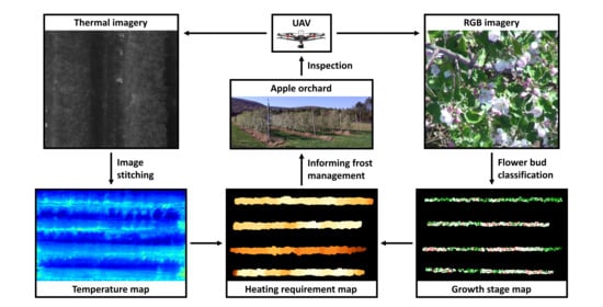
:Frost is a natural disaster that can cause catastrophic damages in agriculture, while traditional temperature monitoring in orchards has disadvantages such as being imprecise and laborious, which can lead to inadequate or wasteful frost protection treatments. In this article, we presented a heating requirement assessment methodology for frost protection in an apple orchard utilizing unmanned aerial vehicle (UAV)-based thermal and RGB cameras. A thermal image stitching algorithm using the BRISK feature was developed for creating georeferenced orchard temperature maps, which attained a sub-centimeter map resolution and a stitching speed of 100 thermal images within 30 s. YOLOv4 classifiers for six apple flower bud growth stages in various network sizes were trained based on 5040 RGB images, and the best model achieved a 71.57% mAP for a test dataset consisted of 360 images. A flower bud mapping algorithm was developed to map classifier detection results into dense growth stage maps utilizing RGB image geoinformation. Heating requirement maps were created using artificial flower bud critical temperatures to simulate orchard heating demands during frost events. The results demonstrated the feasibility of the proposed orchard heating requirement determination methodology, which has the potential to be a critical component of an autonomous, precise frost management system in future studies.
1. Introduction
Extreme weather conditions have always been a major reason for agricultural production loss [1]. With the consideration of global climate changes, it is expected that crop production will be more vulnerable because of the anticipated increase in the extent and frequency of hazardous weathers [2]. As one of the agroclimatic risks that is detrimental to crops, frost represents the main cause for weather related damages in agriculture. Visible frost (“white” frost) forms when water vapor in the atmosphere touches surfaces with temperatures below dew point and freezing point, while invisible frost (“black” frost or freeze) can also happen to plants when air temperature is subfreezing and humidity is low [3,4,5]. Due to sudden cold air invasions or the radiative cooling of Earth’s surface, early spring and late fall are the major time periods for frost events [6], and crops can be injured through freeze-induced dehydration and mechanical disruption of cell membranes caused by ice crystals [7,8]. In the United States, frost has caused more economic losses than any other weather-related phenomenon and often devastates local economies [5]. The degree of frost damage is dependent on many factors including rate of temperature drop, cloud and wind conditions, frosting duration, and crop growth stage [9]. Generally speaking, certain crop developmental stages are more vulnerable to coldness, such as flowering or grain filling. For fruit trees, fruit quality can be greatly influenced by just light frost, while in extreme cases harvesting can even be threatened by severe frost events. During apple blossoming periods, for example, temperatures that are a few degrees below freezing point are adequate to harm or kill flower buds [10], and injured blossoms typically do not develop into fruits.
Frost damage in orchards can be avoided or minimized by active or passive protection methods. Examples of passive methods include site and plant selection, cold air drainage, soil and plant covers, etc. [5]. They are typically less costly than active methods, yet often insufficient to protect crops under severe frost conditions. Active methods can be implemented right before or during a frost event to prevent the formation of ice within plant cells. Sprinklers, wind machines, and heaters are common equipment for active frost protection [11]. As one of the oldest methods, directly adding heat to air with enough heaters under proper weather conditions has the potential to replace substantial energy losses during frost events. Traditionally, orchard thermometers inside instrument shelters are used for orchard temperature monitoring during heating, and, if possible, orchardists adjust the heating level accordingly to keep an air temperature above the critical temperature of the current crop growth stage. However, such a technique of determining orchard heating needs has a few noteworthy shortcomings. First, the number of thermometers being used in an orchard is a limiting factor for how precise the orchard temperature can be managed spatially. Second, humans are required for checking thermometers to ensure ample heating as well as to prevent overheating, which can be laborious and untimely. Third, plant tissue temperature may differ from air temperature, and readings of orchard thermometers do not necessarily reflect true orchard heating demands. Last, spatial plant growth stage variation in an orchard is typically ignored. It is wasteful to maintain the same temperature throughout an orchard, as critical temperatures vary with plant developmental stages [12]. Following the trend of precision agriculture [13], a modernized methodology of heating requirement determination for frost management in orchards that can assess localized, actual heating needs while considering spatial plant growth stage variability and keeping human involvement to the minimum would be desirable.
The fast development of unmanned aerial vehicles (UAVs) and relevant remote sensing technologies in recent years brings new opportunities for their applications in agricultural management tasks [14]. It is believed that UAVs will be an essential part of precision agriculture in the future [15]. Potentially, missions such as plant growth stage classification and plant temperature monitoring could be efficiently accomplished by UAV-based sensors such as cameras. Aerial thermal cameras, which measure heat through infrared radiation, have been applied in research for a wide range of crops such as citrus [16], grape [17,18], almond [19], maize [20], soybean [21], and sugar beet [22]. Canopy temperature information is typically used for crop water status assessment as it is a function of available soil water and plant transpiration rate [23]; moreover, it has been reported to be correlated with other crop traits such as lodging [24], biomass [25], and yield [26]. Due to hardware limitations, e.g., field of view (FOV), monitoring large orchard temperatures with an airborne thermal camera may require a high flight altitude, resulting in an increase in image spatial resolution and compromised image details [27,28]. Such an issue can be solved by transforming multiple overlapping images into one mosaic with well-established image stitching techniques [29], although thermal image stitching is a less popular topic than red, green, and blue (RGB) image stitching. RGB cameras, on the other hand, play a crucial role in remote sensing since images in the visible spectrum represent agricultural environments well, which makes them ideal instruments for helping identify crop reproductive organs at different growth stages. Object detection is a common computer vision problem that deals with the localization and classification of target objects in images, while newly emerged convolutional neural network (CNN)-based algorithms such as R-CNN series (R-CNN [30], Fast R-CNN [31], Faster R-CNN [32], Mask R-CNN [33], Libra R-CNN [34], etc.) and YOLO series (YOLO [35], YOLOv2 [36], YOLOv3 [37], YOLOv4 [38], etc.) have achieved successes even in the agriculture domain. For instance, Grimm et al. [39] detected shoots, flower buds, pedicels, and berries of grape with a semantic segmentation framework; Chen et al. [40] adopted Faster R-CNN for identifying flowers and immature and mature fruits of strawberry; Koirala et al. [41] compared five CNN-based algorithms on classifying three mango panicle stages; Milicevic et al. [42] distinguished open and non-open flowers of olive based on a custom CNN; Ärje et al. [43] classified buds, flowers, wilted flowers, and seed pods of Dryas integrifolia using three CNN models; and Davis et al. [44] counted buds, flowers, and fruits of six wildflower species with Mask R-CNN. Despite the fact that several studies have utilized the deep learning approach for classifying plant developmental stages, it is still an underexplored topic as the difficulty of object detection tasks can vary greatly for different plants and environments depending on factors such as scene disorderliness, object positioning, and object occlusion [45], which remain unknown for many species such as apple.
In this article, we aimed to demonstrate the concept of UAV-based apple orchard heating requirement determination for frost protection in a high resolution, low time cost fashion. Specifically, the three objectives of the study were (1) developing an algorithm that generates georeferenced orchard temperature maps based on thermal image stitching, (2) building a CNN-based classifier for apple flower bud growth stages and implementing the classifier to create orchard flower bud growth stage maps, and (3) simulating orchard heating requirement maps in terms of how many degrees tree temperatures must go up for flower buds to not have damages during frost events based on the aforementioned maps.
2. Study Site, Equipment, and Data Collection
Field experiments were conducted in Russell E. Larson Agricultural Research Center, Pennsylvania Furnace, Pennsylvania, USA. The apple orchard was roughly 25 m long and 15 m wide (40.707918° N, 77.954370° W in WGS 84 datum). It was originally planted in 2008 and consisted of four rows and two cultivars including Jonagold and Daybreak Fuji, with 16 trees in each row and two rows for each cultivar. Tree spacing inside each row was approximately 1.7 m and row spacing was approximately 4 m. The trees were mechanically pruned into hedgerow and the average tree height was around 2.7 m.
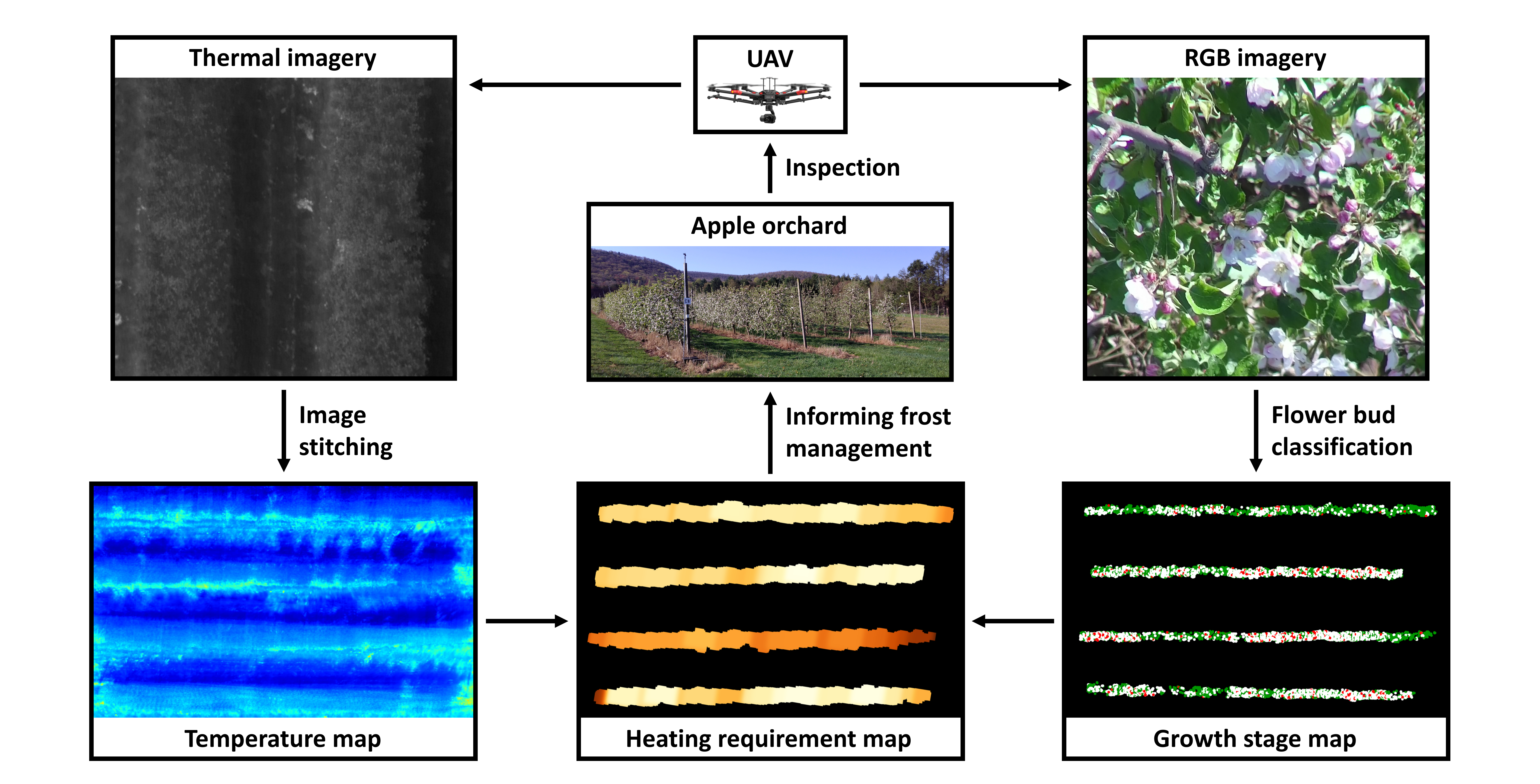
We had the following consideration in mind when deciding hardware suitable for the study and practical usage. First, the UAV needed to have a high payload to carry heavy instruments such as cameras while maintaining a reasonable hovering time. Second, aside from the thermal camera must have radiometric functionality, a high thermal image resolution could help create detailed orchard temperature maps. Last, the RGB camera should have an exceptional zooming capability to capture high definition images of apple flower buds, as the UAV must fly above a certain altitude to not cause turbulence near trees and prevent buds from being blurry in images. Our final selection for the equipment included Matrice 600 Pro, Zenmuse Z30, and Zenmuse XT2 from DJI (China) (Figure 1), and their key specifications are listed in Table 1.
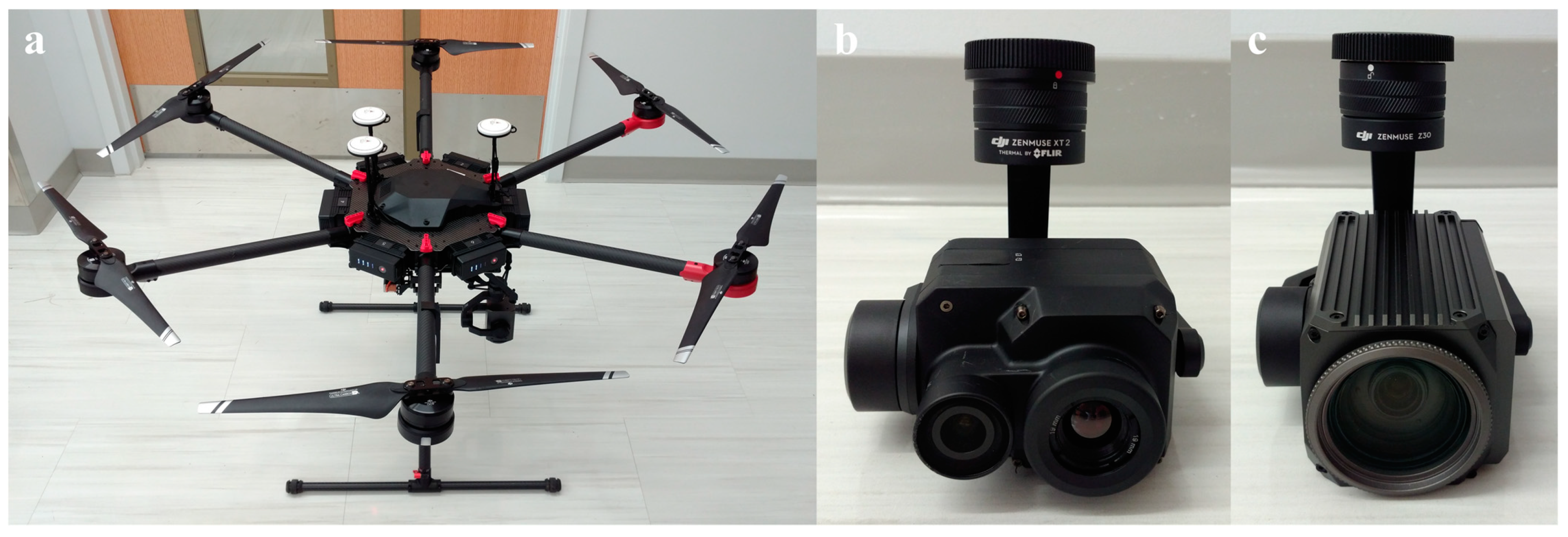
Two types of data were collected in the growing season of 2020, including sets of thermal images covering the whole orchard for generating temperature maps and apple flower bud RGB images at various growth stages for the training and application of a CNN-based object detector. For thermal missions, flight altitude was set at 20 m above ground level (AGL) to mitigate parallax error [46], and the UAV flew at 1 m/s while the thermal camera captured images every 2 s with a 90° pitch. Approximately 100 thermal images were captured in 4 min during each fully autonomous flight and saved in tiff format, and the images had a 75% front overlap and a 70% side overlap. The thermal datasets used for demonstration in this article were collected on June 2, 2020. The RGB images were captured with the RGB camera’s full optical zooming capability, a fixed focus to tree canopy top, and a 90° camera pitch. Except for the first data collection date when a 10 m AGL flight altitude was adopted, the UAV flew at 15 m AGL with a manual speed no higher than 0.1 m/s to ensure image sharpness. A semi-autonomous RGB mission required 40 to 90 min to complete, when 600 to 1100 images in jpg format were captured, and the UAV’s flying altitudes were maintained automatically by DJI’s A3 Pro flight control system. RGB data collected on the 19th, 23rd, 28th of April, 2020, the 2nd, 7th, 13th, 16th, 21st of May, 2020, and the 24th of September, 2020 were used for model training. RGB and thermal flight missions shared a similar flight path as shown in Figure 2.
3. Methods
3.1. Thermal Camera Radiometric Calibration
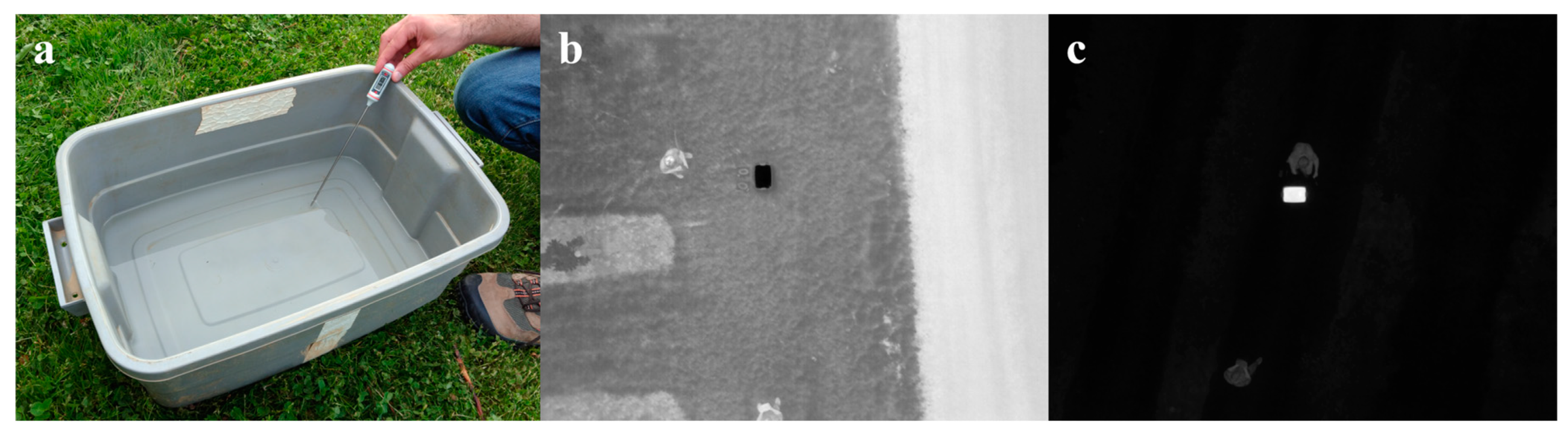
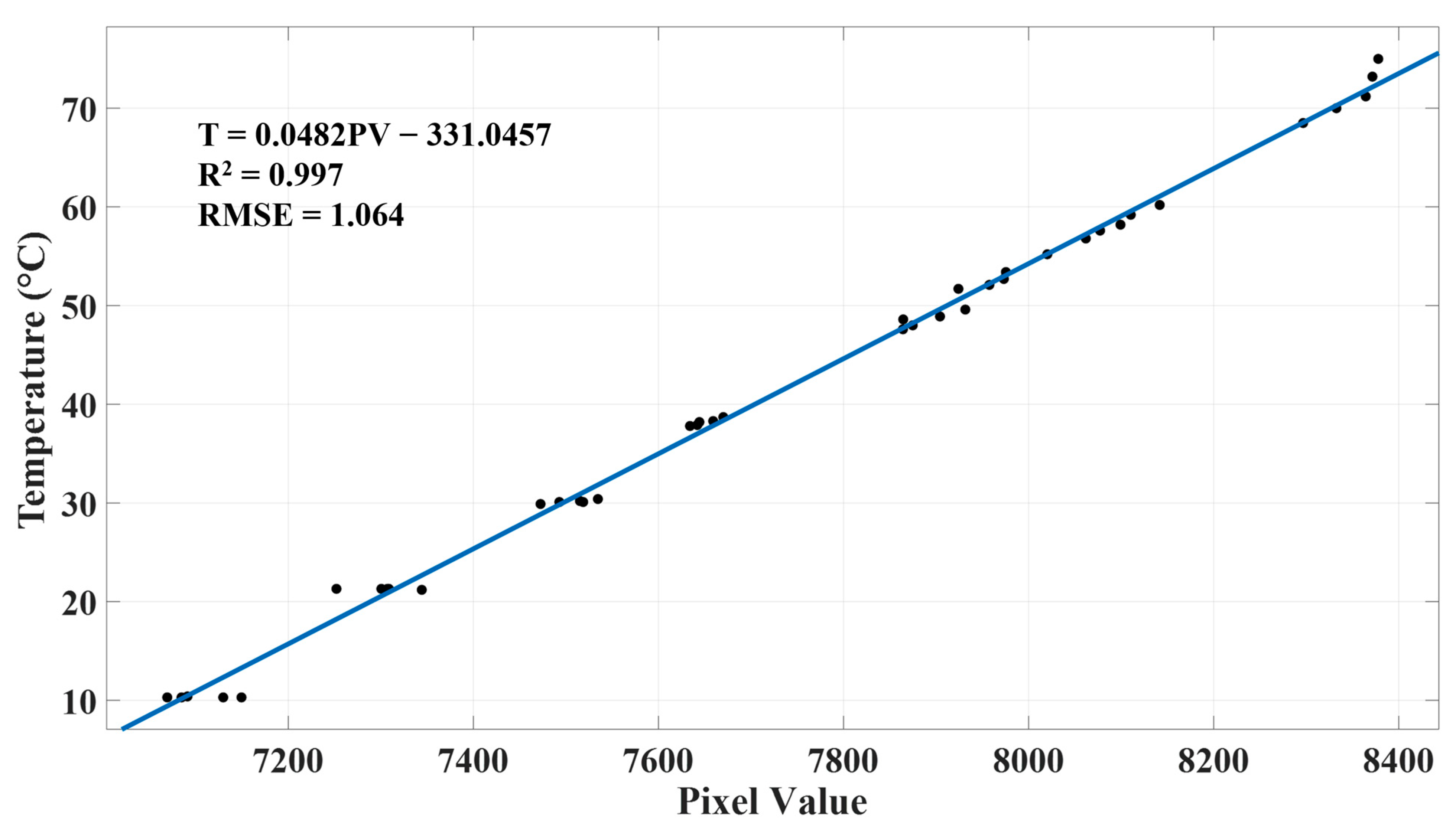
An aerial thermal camera needs to be calibrated before data analysis as its accuracy could be affected by factors such as target object properties and flight altitude [47]. Atmosphere-induced radiometric distortion can be considered negligible under low flight altitude changes [48]; therefore, object surface emissivity was the major variable that needed to be calibrated for in the study. As typical green leaves, such as apple leaves, have a thermal emissivity of 0.95 [49], and pure water has a similar emissivity of 0.97 to 0.99 in the spectral range of 8 to 13 µm with observing zenith angle in between 0° to 30° [50], a plastic container filled with tap water at various temperatures was used as the calibration target. The water temperatures were measured by a digital thermometer (9329H03, Thomas Scientific, USA) with an accuracy of ±0.2 °C. Thermometer readings of water were recorded once they stabilized; meanwhile, thermal pictures were taken by the UAV at a 20 m altitude with a 90° camera pitch mimicking a thermal flight mission (Figure 3). In total, 40 pairs of thermometer readings and thermal images were collected. Non-water pixels in each thermal image were first cropped out, and the mean of water pixel values was then computed and used for calibration. On average, each cropped image had approximately 200 water pixels. The relationship between pixel intensity and water temperature was estimated using robust least-squares regression with bisquare weights.
3.2. Thermal Image Stitching
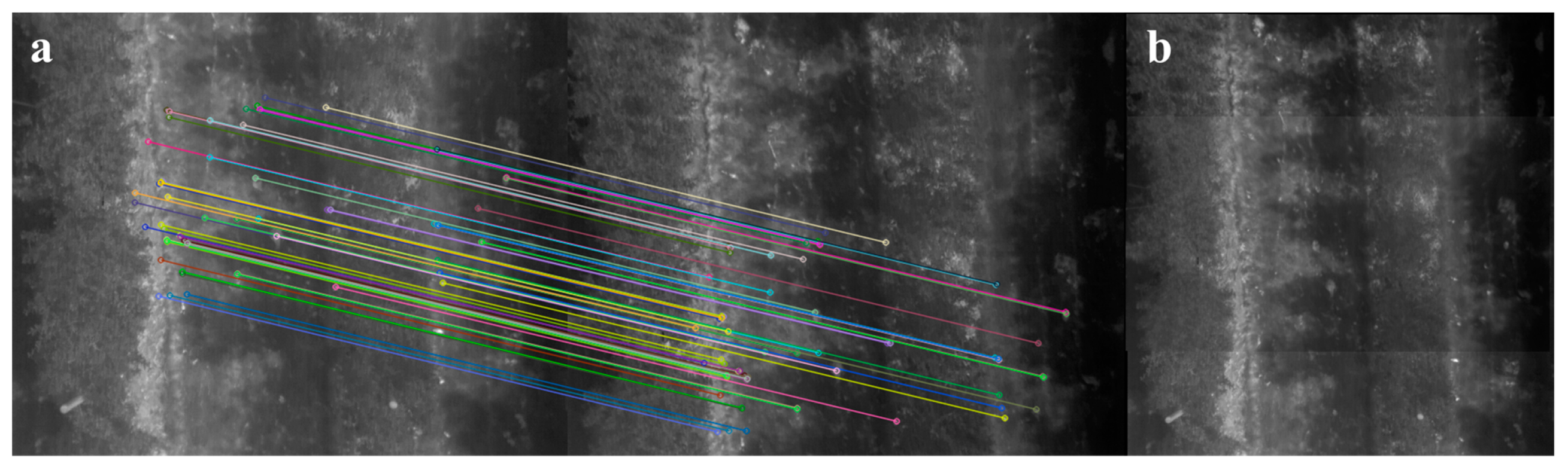
The generation of an orchard temperature map requires individual thermal images to be first stitched into a mosaic. However, typically thermal images are more difficult to register than RGB images due to their lower resolutions and fewer image details [51]. In this study, we adopted a feature-based approach to address this issue. Instead of choosing commonly used algorithms such as SIFT [52] or SURF [53], we implemented BRISK [54] as the method for image feature detection and description. BRISK identifies image keypoints through the FAST detector [55] on octaves in an image pyramid and a non-maxima suppression by comparing a point of interest to its neighboring points on the same octave as well as corresponding points on the neighboring octaves. BRISK describes a circular sampling area of a keypoint in a binary manner with scale and rotation normalized. It has been reported that BRISK had a better computational efficiency and a comparable accuracy than SIFT for image registration [56].
The image stitching algorithm was developed in Python with OpenCV [57] and scikit-image [58]. Its general workflow is described as follows. For any pair of images taken consecutively, the BRISK keypoints and descriptors of the two images are computed. Pairwise Hamming distances [59] between descriptors are calculated exhaustively, and each query descriptor is considered to have a match when the distance ratio between the closest and the second closest neighbor is smaller than 0.8 as suggested by Lowe [60]. The transformation between two image planes is assumed to be 2D Euclidean considering the images were taken with fixed UAV flight altitude and camera pitch. All pairwise homographies are estimated through RANSAC [61] within 100 iterations, where each random data subset contains four pairs of matches, and the maximum distance for a keypoint to be classified as an inlier is set as two pixels. Anchor homographies are calculated by pairwise homography multiplication. Image stitching is achieved by warping non-anchor images based on their anchor homographies and overlaying them to the anchor image (Figure 4). The intensities of all overlapping pixels are averaged in the stitched mosaic.
3.3. Thermal Mosaic Georeferencing
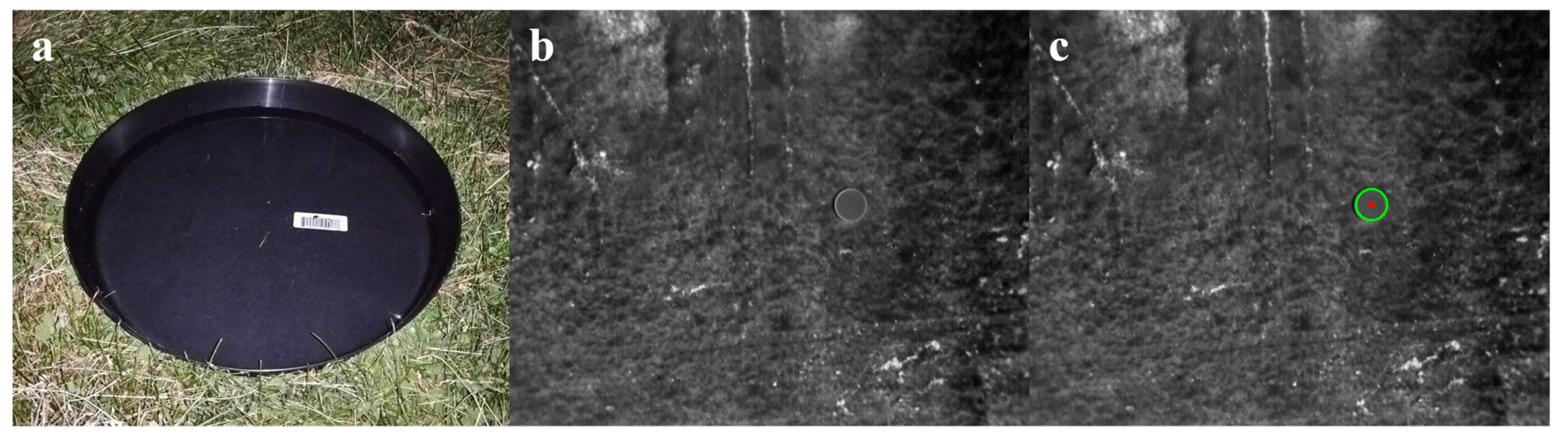
Three plastic saucers filled with room temperature water were used as ground control points (GCPs) for georeferencing thermal mosaics, which appeared as circles with relatively uniform pixel intensities in the thermal images hence were easy to detect. The saucer diameters varied from 0.46 to 0.63 m, and the size difference allowed them to be later identified uniquely during image processing. The saucers were placed around the orchard edge, and their GPS coordinates were measured by a pair of global navigation satellite system (GNSS) modules (Reach Module, Emlid, China) with single-band antennas (TW4721, Tallysman, Canada). As the outputs of GNSS modules always carry a certain level of noises, to achieve better location estimations, for each saucer 900 to 1000 latitude and longitude readings of the saucer center were recorded at a 5 Hz GPS update rate, and the median values were taken as the saucer center coordinates to avoid potential outliers. Our tests showed that the saucer GPS measurements attained an accuracy of ±0.13 m. 2–1 Hough transform [62] was implemented in Python as the method for saucer detection. During georeferencing, pre-measured GPS coordinates were assigned to the center pixels of detected saucers (Figure 5), and least-squares fitting-based first-order polynomial transformation was utilized for converting rows and columns of raster thermal mosaics to coordinate maps.
3.4. Flower Bud Growth Stage Classification
Apple flower buds are usually considered to have nine growth stages including silver tip, green tip, half-inch green, tight cluster, first pink, full pink, first bloom, full bloom, and petal fall [63]. As the transition of buds from one growth stage to another is a gradual process, we observed that it could be very difficult to distinguish certain growth stages from one another in the RGB images. As the neighboring stages have either identical or close critical temperatures [63], we created a six-class system for the apple flower bud classification that merged certain growth stages (Table 2). As the critical temperatures of Jonagold and Daybreak Fuji remain unknown in current literature, we adopted Red Delicious’ critical temperatures for both apple varieties as a reference [63]. Note that, aside from growth stage, plant variety also has an influence on plant cold tolerance, and one should consider vegetation heterogeneity for the most precise orchard temperature management. As a clarification, in this article a flower “bud” refers to the complete structure of what a flowering tip develops into, such as a flower cluster with several flowers and numerous leaves; a “flower” refers to an unbloomed pink flower in pink stage, a bloomed white flower in bloom stage, or a petal-less flower in petal fall stage.
Typically, CNN-based models rely on supervised learning, meaning “ground truths” need to be prepared by experts such as labels of target objects in an image. However, there were several factors that posed challenges to the image annotation process for this study. First, as mentioned above, the development of buds happens in a gradual manner, and buds oftentimes do not possess enough distinct characteristics to be classified in a certain growth stage, which adds difficulties to the decision-making during bud labeling. Second, because of the training systems adopted for the orchard, apple trees can have a dense 3D distribution of buds and flowers that grow closely to each other, which creates confusing scenes for humans to identify a complete flower bud in 2D images. Third, vegetative buds can be mistaken as flower buds [65], especially the ones before tight cluster stage. Fourth, an apple flower bud grows from a tiny tip into a flower cluster containing multiple flowers and leaves, which involves a significant size change. Identifying flowers and leaves that belong to the same bud could be demanding and impractical. Last, as the RGB images were taken by an aerial camera observing a small area, any slight movements of the trees or the UAV could lead to reduced image quality. To address these issues, we determined several criteria as the guidance for bud labeling in various scenarios:
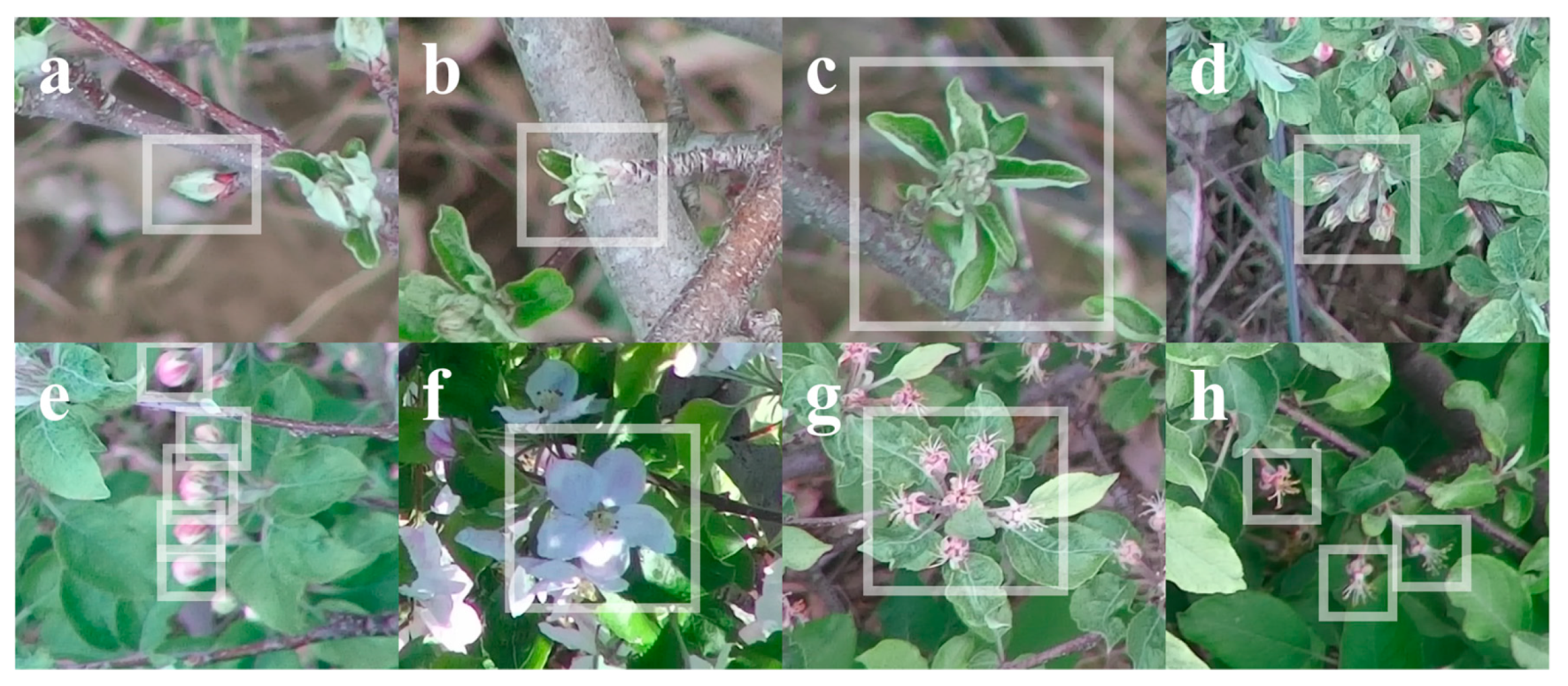
- For stages at or before tight cluster, include the whole bud in a bounding box. For stages at or after pink, exclude leaves from a bounding box (Figure 6).
- For stages at or before tight cluster, each bounding box should contain only one bud (Figure 6a–c). For pink or petal fall stage, if the flowers that belong to the same bud are recognizable and relatively close to each other, label all flowers in the same bounding box (Figure 6d,g); otherwise, label each flower with a bounding box (Figure 6e,h). For bloom stage, each bounding box should contain only one flower (Figure 6f).
- When knowing a bud or flower exists but the complete shape of it cannot be identified, due to image blurriness or dense flower bud distribution, do not label.
- When having doubts whether a bud is a leaf or flower bud, do not label.
YOLOv4 [38], a state-of-the-art CNN-based object detector, was deployed for the apple flower bud growth stage classification task. It is capable of operating in real-time on a conventional GPU and has been demonstrated to have a high performance on the Microsoft COCO dataset [66]. The model architecture consists of a CSPDarkNet53 [67] backbone with Mish activation [68], a neck of SPP [69] and PANet [70] with Leaky activation, and a YOLOv3 head. To improve class balance, instead of using all the collected images, 450 positive samples containing at least one bud or flower were arbitrarily selected from each of the eight datasets collected in April and May, 2020 for labeling. The image annotations were prepared in Darknet format using an open source tool YoloLabel [71] by a two-stage process, where the images were first labeled by the first author and four trained research assistants, and then double-checked and relabeled only by the first author for unlabeled buds, mistaken labels, and labeling style inconsistency. Annotated images of each date were split into 70%, 20%, and 10% segments for model training, validation, and test, respectively. An equal amount of negative samples containing no bud or flower, which were captured mostly in September, 2020, were also added to the training dataset to improve model robustness. In total, the training, validation, and test datasets consisted 5040, 720, and 360 images, respectively.
The classifier trainings were executed on a computer with an Intel® Core™ i9–9900 (USA) CPU, an NVIDIA GeForce RTX 2060 (USA) GPU, and a 16 GB RAM. Three network sizes were experimented with: 320, 480, and 640. Except for learning rate, which was manually tuned between 0.002 and 0.00001 during training to prevent overfitting, all other hyperparameters were adopted as default. Average precisions (APs) of a class were calculated based on 11-point interpolated precision–recall curves [72], while the trainings were stopped when the mean average precisions (mAPs) of the validation dataset no longer improved. Model weights with the highest validation mAPs were selected for further evaluation on the test dataset.
3.5. Flower Bud Location Calculation
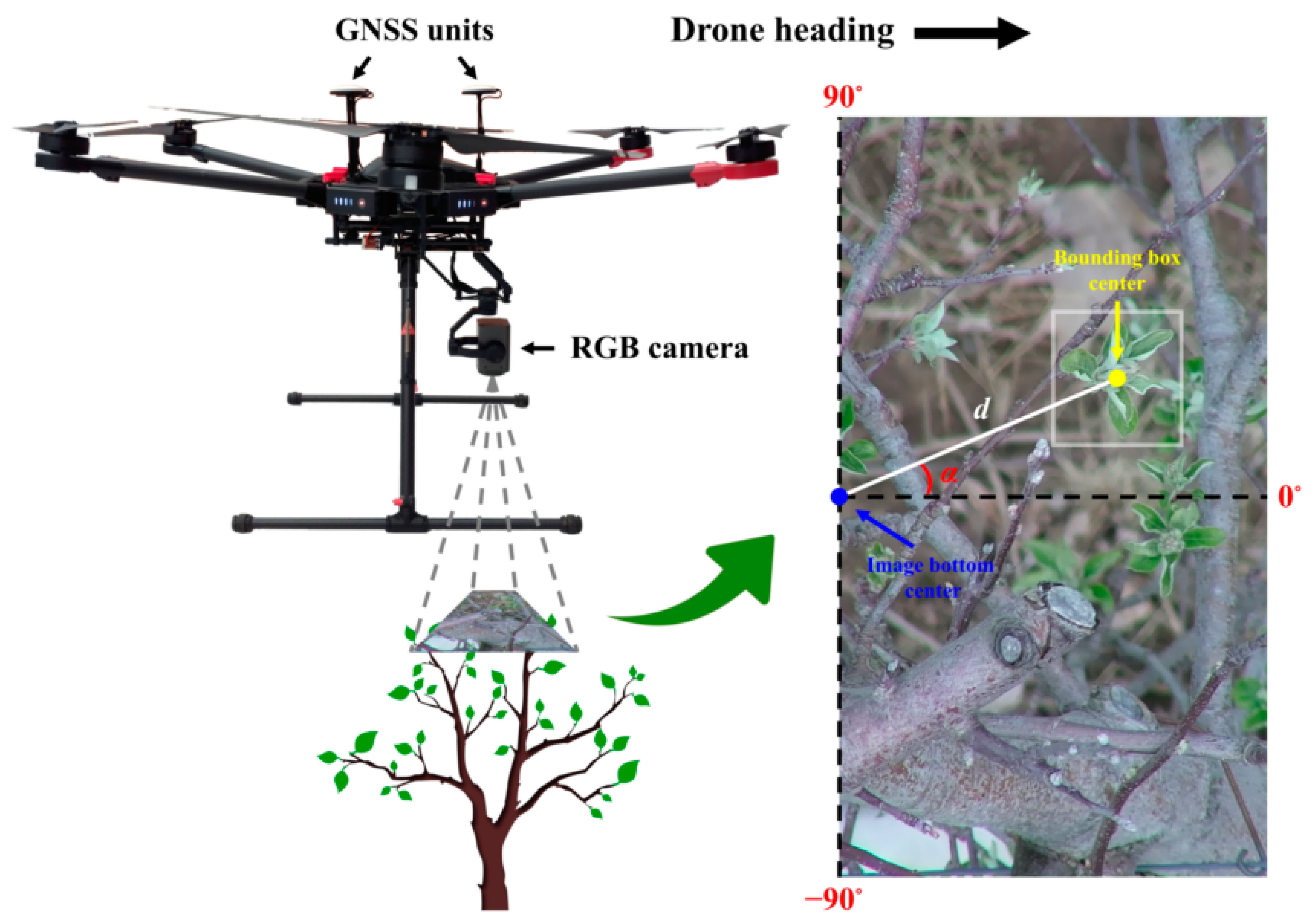
Every RGB image collected in the study was geotagged by DJI’s A3 Pro flight control system. For mapping purposes, the GPS coordinates of each image were utilized for georeferencing the flower buds in the image detected by the classifier. As the camera was fixed at a front position relative to the UAV’s GNSS units along the drone heading direction, the GPS coordinates of an image represented a point at a rear position relative to the image center. Considering the small offset between the GNSS units and the RGB camera as well as the narrow tele-end FOV of the camera, to simplify flower bud location calculation, the GPS coordinates of an image were assumed to represent the location of the image bottom center point (Figure 7). Based on the relative position of a bud in an image, the latitude and longitude of the bud were calculated in Python using the following formulas [73] ignoring Earth’s ellipsoidal effects,
where φ1 is the latitude of an image bottom center, λ1 is the longitude of an image bottom center, φ2 is the latitude of a bounding box center, λ2 is the longitude of a bounding box center, θ is the bearing from image bottom center to bounding box center, and δ is the angular distance between image bottom center and bounding box center. θ is determined by subtracting the “zenith” angle α from the drone heading. If θ is larger than 180°, an additional 360° needs to be subtracted to keep θ in the −180° to 180° range. On average, the drone heading was either 151.33° or −28.67° during RGB flight missions depending on the tree row. α ranges from −90° to 90°. δ is calculated as d/R, where d is the distance between image bottom center and bounding box center, and R is Earth’s average radius being 6,371,000 m. Given UAV flight altitude, average tree height, image resolution, and camera FOV, the area of each RGB pixel was computed to be approximately 6.60 × 10⁻⁸ m2, and d is further derived from the pixel numbers in between image bottom center and bounding box center (Figure 7).
φ2 = asin(sin(φ1)⋅cos(δ) + cos(φ1)⋅sin(δ)⋅cos(θ)),
λ2 = λ1 + atan2(sin(θ)⋅sin(δ)⋅cos(φ1), cos(δ) – sin(φ1)⋅sin(φ2)),
3.6. Regional Heating Requirement Determination
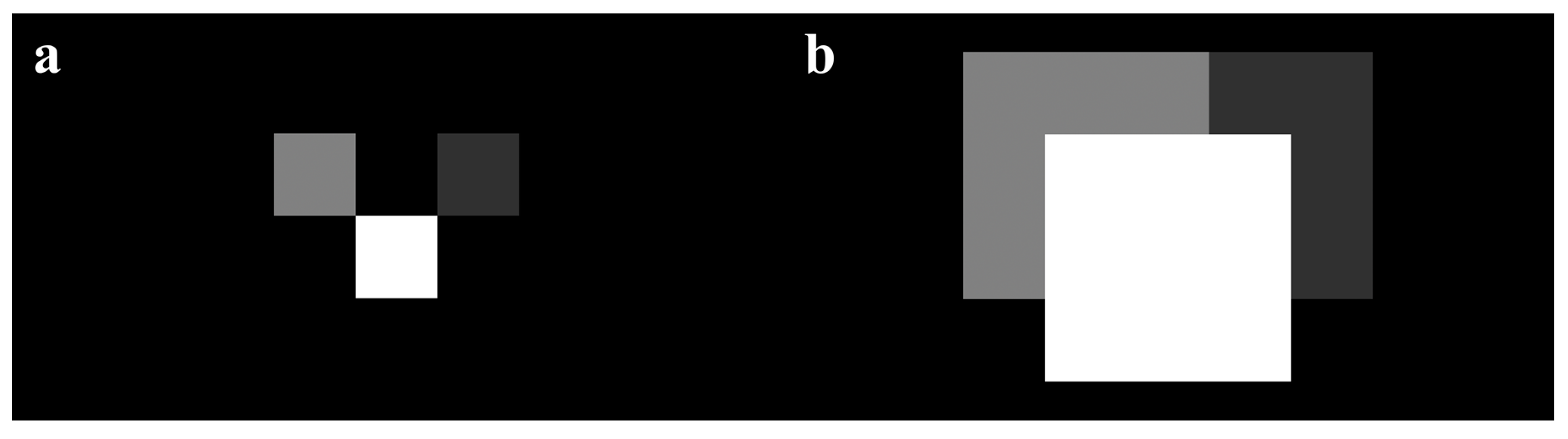
Given detected bud coordinates and a georeferenced thermal mosaic, apple flower buds at various growth stages can be mapped as pixels with unique colors onto the coordinate map, representing different critical temperatures. Orchard heating requirement maps could be calculated by simply subtracting temperature maps from critical temperature maps, where pixels indicate the heating needs at detected bud locations. Yet, such maps will not be viewing-friendly and practical for usage, as heating needs of individual buds are not directly helpful for orchardists to determine heating treatments of a region. To solve this issue, we simplified our heating requirement maps by dilating heating requirement pixels and “prioritizing” pixels with higher intensities representing higher heating demands (Figure 8), which allowed humans to conveniently see the highest possible heating needs of a region. For this study, each detected bud was initially mapped as one pixel before dilation. As we did not have a chance to collect a thermal dataset when tree temperatures were below critical temperatures, we simulated heating requirement maps by employing a temperature map and a flower bud growth stage map from two dates, and artificial critical temperatures to demonstrate the concept.
4. Results and Discussion
4.1. Thermal Camera Calibration Results
Our regression analysis of thermal pixel intensity and ground truth temperature resulted a strict linear relationship with an R2 of 0.99 and an RMSE of 1 °C (Figure 9), which is similar to what many relevant studies obtained for airborne thermal imagers, such as R2 of 0.98 and RMSE of 1.53 °C for ICI 8640 P-Series (USA) [74], R2 of 0.98 and RMSE of 1.9 °C for ICI 9640 P-Series [75], R2 of 0.93 and RMSE of 0.53 °C for senseFly thermoMAP (Switzerland) [76], and R2 of 0.96 [48] and 0.937 [47] for FLIR Vue Pro R 640 (USA).
Generally, thermal cameras can be divided into two categories: cooled and uncooled [77]. Modern drone thermal cameras such as the ones mentioned above are typically equipped with uncooled detectors such as microbolometers [78]. Uncooled cameras have advantages such as light weights, small sizes, and low prices, which make them an ideal choice for many UAV applications [79]. However, they have higher thermal time constants and are known to suffer from thermal noises induced by changes in camera body temperature [80]. Although being expensive, cooled thermometers usually have greater magnification capabilities, better sensitivities, and are able to capture sharp images under short integration time. As a thermal camera can be interfered with by its surroundings, thermal calibration results should be utilized as mission-specific when significant environmental changes are involved, such as air temperature, humidity, and flight altitude [81]. Nevertheless, the capacity and accuracy of an uncooled thermal camera are sufficient for our application of orchard temperature monitoring, while cooled thermal cameras seemingly have the potential to be a superior option when future technology matures.
4.2. Thermal Mosaic and Orchard Temperature Map
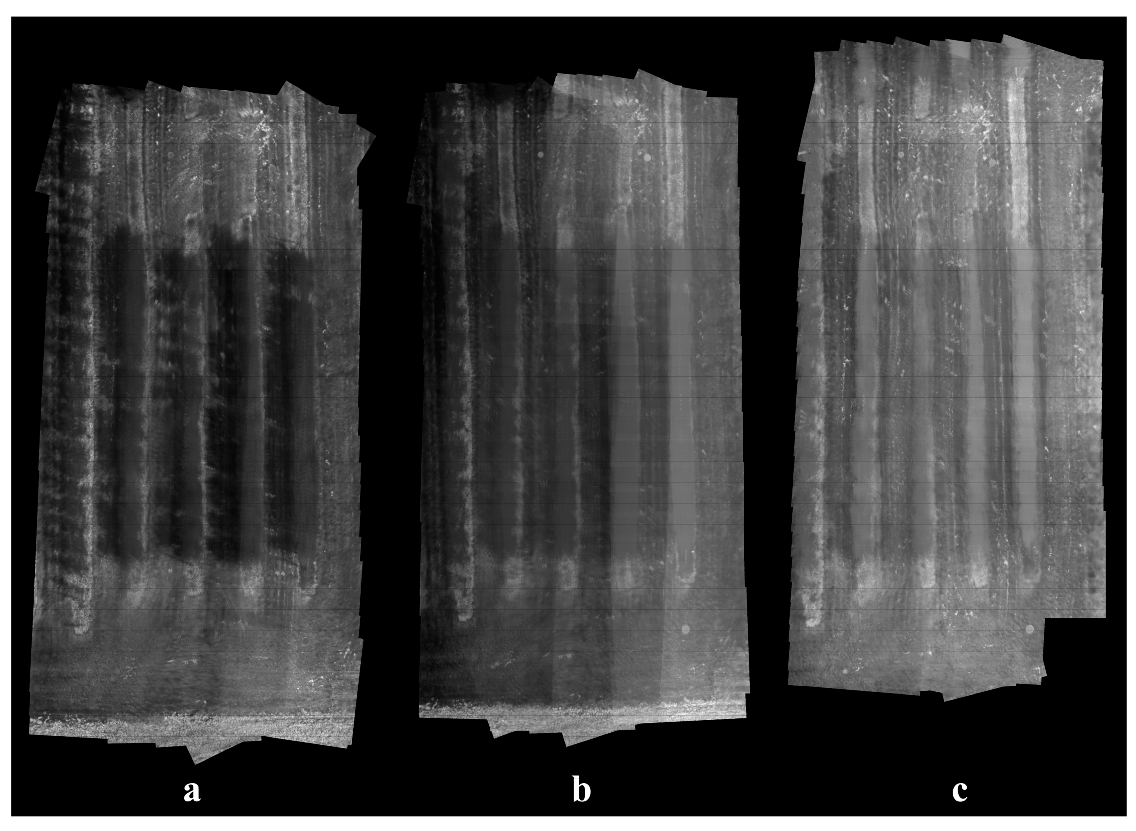
Running on the same computer for the classifier training, our stitching algorithm was able to generate a mosaic from a dataset of 100 thermal images within 30 s on average. The stitching results were satisfactory as all apple trees could be clearly distinguished from background, although certain levels of blurriness and misalignment existed due to parallax effect and lens distortion. For demonstration purposes, only a minimum amount of GCPs was employed in this study, while higher overall accuracy of coordinate maps can be achieved with more GCPs, allowing complex image distortion to be corrected with higher order transformations. Generally, sunlight helps robust stitching by creating shadows and improving image contrast, as the temperature difference between plants and soil increases under sun exposure, and more distinctive image features can be detected and matched. Conversely, rapidly changing weather conditions can bring challenges to the stitching process when temperatures of the same objects differ significantly in two images. Although sunny weather is a favorable condition, the absence of direct sunlight did not cause difficulty to image stitching in this study, and thermal images taken at night-time and cloudy daytime were expected to share similar appearances. On average, 976 BRISK keypoints were detected in each image from the cloudy dataset (Figure 10c) and 341 were matched in an image pair. In contrast, the two numbers were 1162 and 428 for images from the sunny dataset (Figure 10a).
Customization of thermal image stitching is much less studied compared to RGB image stitching. Teza [82] developed a MATLAB toolbox that was capable of registering thermal images for wall damage recognition using Harris corner detector. Wang et al. [51] reported a framework for stitching video frames from aerial thermal cameras based on SIFT. Sartinas et al. [83] proposed a robust video stitching method for a UAV forest fire monitoring utilizing ECC algorithm [84]. Besides using SIFT [85], Semenishchev et al. [86] also employed contour centers as keypoints for stitching quantized thermal images. In the agriculture domain, many researchers chose commercial software such as Pix4D (Switzerland) [48,74] or Agisoft Metashape (Russia) [75,79] for UAV thermal image mosaicking, which is convenient for inexperienced programmers and generally can produce robust results. Our customized algorithm has the advantage of being flexible in modifying its components. For example, the BRISK feature can be easily changed into newer state-of-the-art image feature detectors and descriptors. It is possible to improve the final stitching results by applying techniques such as lens distortion correction [87], bunding adjustment [29], and blending [51]. We excluded these steps to keep the algorithm as simple and fast as possible, and not to make unnecessary pixel value manipulations hence preserving original temperature measurements.
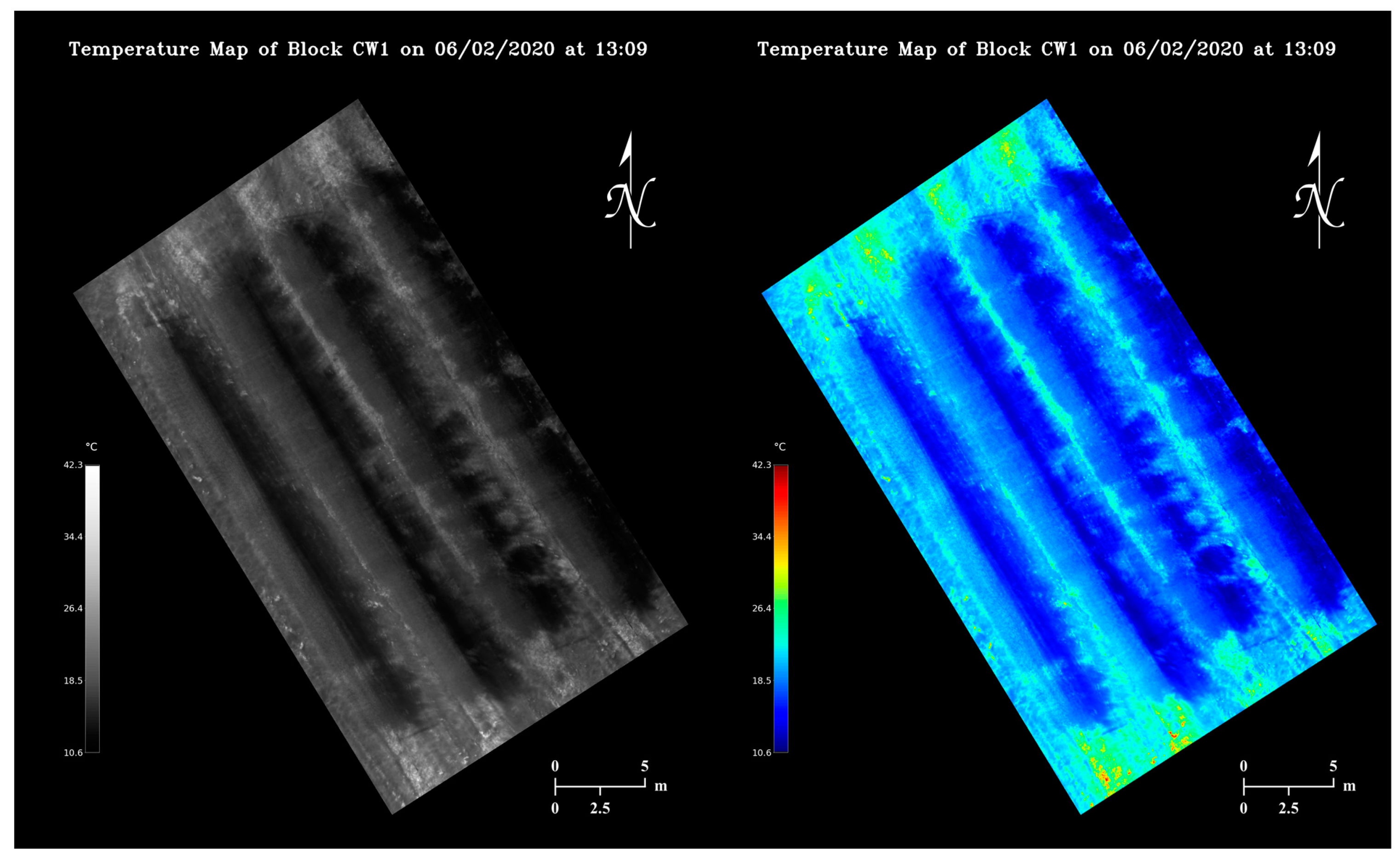
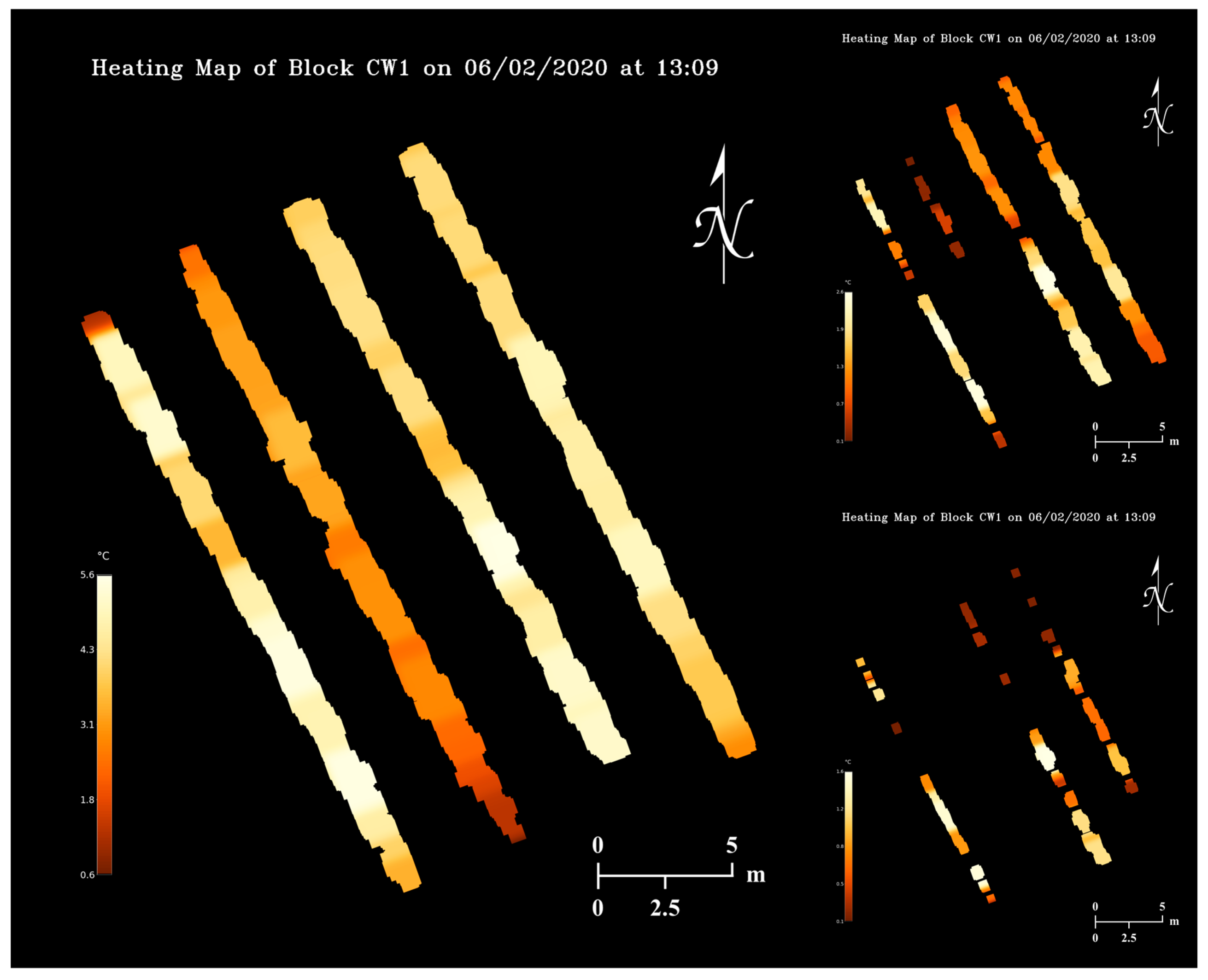
Utilizing the calibrated pixel value-temperature relationship, viewing-friendly maps containing orchard temperature information could be generated from thermal mosaics at a negligible time cost as shown in Figure 11. Each pixel in the maps covers an area of 3.23 × 10⁻⁴ m2 approximately. Note the maps reflect orchard temperature changes in a 4-minute window. Under a partially sunny condition, certain regions of a map can appear substantially darker or brighter than the rest (Figure 10b).
Flight time and stitching time are two important factors that govern how timely orchard temperature can be managed using our methodology. Currently our image collection and algorithm execution together could cause a minimum 5-minute delay from real time temperature monitoring. As we already prioritized the computation simplicity when designing the stitching algorithm, optimizing UAV flight missions has more potential in improving map generation speed, which essentially is a trade-off between orchard temperature monitoring resolution and timeliness. At a higher altitude, faster UAV flying speeds can be adopted as a larger area will be covered in each image, and motion blur would be less problematic. The maximum speed of our UAV is up to 15 m/s, with which a thermal flight mission could be completed within 30 s. As trees growing next to each other tended to have similar temperatures (Figure 11), much lower temperature map resolutions, for instance, even if each thermal pixel covers a whole tree, could still be potentially sufficient for determining orchard regional heating needs, in which case only a few images need to be taken at a high altitude to minimize flight time in the future.
4.3. Flower Bud Growth Stage Classifier Performance
For each of the three experimented network sizes, APs and mAPs of the best model at 50% intersection over union (IoU) on the validation and test datasets are listed in Table 3. Out of the three network sizes, 320 had the lowest mAP, while 480 and 640 had comparable mAPs, indicating image input resolution higher than 480 might not bring additional useful information to the network training. AP seemed to have a direct correlation with object size. Out of the six stages, tip and half-inch green consistently had the lowest APs, when apple flower buds were the most underdeveloped and had the smallest sizes; pink had considerably lower APs than tight cluster and bloom, while generally it also had smaller bounding boxes as leaves were excluded in pink but included in tight cluster, and flowers were closed in pink but open in bloom; from bloom to petal fall, APs decreased significantly as the absence of petals led to smaller bounding boxes of petal falls than bloom. Due to a smaller sample size, the test dataset showed substantially larger APs of tip and half-inch green than the validation dataset, indicating larger sampling biases.
To our knowledge, deep learning-based apple flower bud growth stage classification has never been studied in existing literature; however, attempts for CNN-based apple flower detection have been made previously. Tian et al. [88] proposed a modified Mask Scoring R-CNN model for classifying three types of apple flowers based on their morphological shape, including bud, semi-open, and fully open. Trained on a dataset of 600 images, out of which 400 were manually collected and 200 were generated through image augmentation, their model achieved a 59.4% mAP on a test dataset of 100 images. Wu et al. [89] identified flowers, or rather stamens, of three apple varieties with a simplified YOLOv4 network. With manually collected 1561 images for training and 669 images for testing, they obtained a 97.31% AP for flower detection.
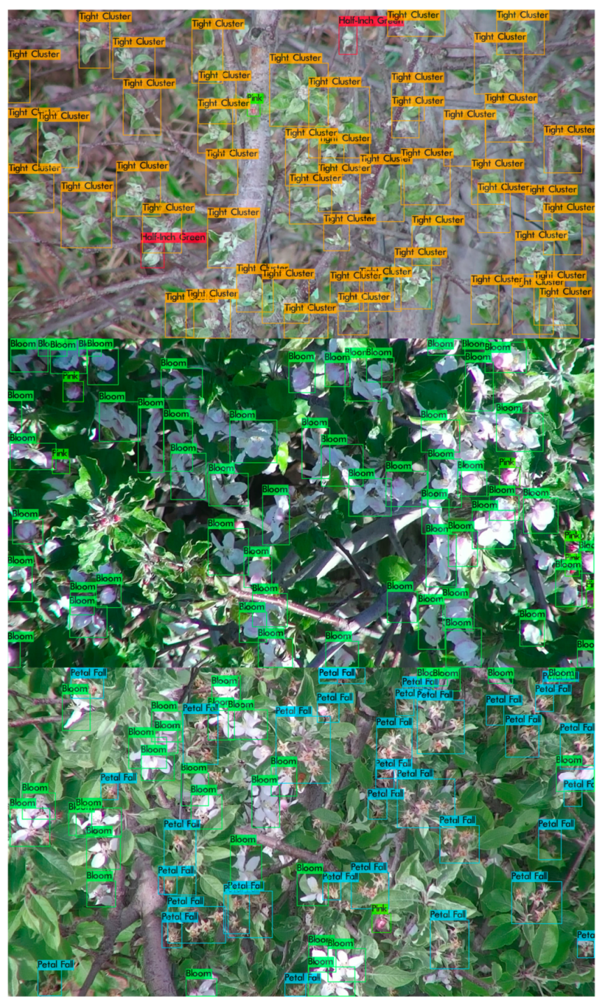
Despite the similarities in nature, we consider our study possess a higher complexity than the two studies reviewed above because of two important factors: data temporal coverage and flower distribution density. The two studies collected data only at a narrow time window, which corresponded to the bloom stage in this study. On the contrary, our datasets captured the full range of apple flower bud developmental changes. During image labeling we had to constantly make judgment calls on which stage a flower bud belonged to, when facing scenarios such as a half-inch green slightly opened up its leaves, a tight cluster started to show light pink color, a pink transitioned from being pinkish to whitish, a bloom wilted or dropped a few petals, etc. The inevitable inconsistency of bud labels, as far as we are concerned, is one of the crucial reasons for the imperfect results of our classifiers. Furthermore, we observed that the sample images provided in the two studies had much lower floral density compared to our images. Using the 450 annotated images collected on May 7, 2020 when buds were mostly blooms as an example, the minimum, medium, and maximum number of bounding box per image were 5, 58, and 112, respectively. The dense bud distribution contributed much difficulty to labeling every single flower bud in an image and recognizing all the deformed, occluded flower buds at various depth correctly during image annotation (Figure 12), which could be another key reason that prevented our classifiers from achieving excellent performances. While building new classifiers with larger image input sizes than 640, or training current classifiers with new images might improve APs for tip, half-inch green, pink, and petal fall, we believe reexamining current image labels for annotation accuracy, consistency, and completeness has a greater potential in helping increase model sophistication, although the process can be very labor-intensive. Considering the average apple flower bud distribution density, suboptimal classifier detection results, such as missing several buds, should have little to no influence on orchard heating requirement determination.
4.4. Orchard Flower Bud Growth Stage Map
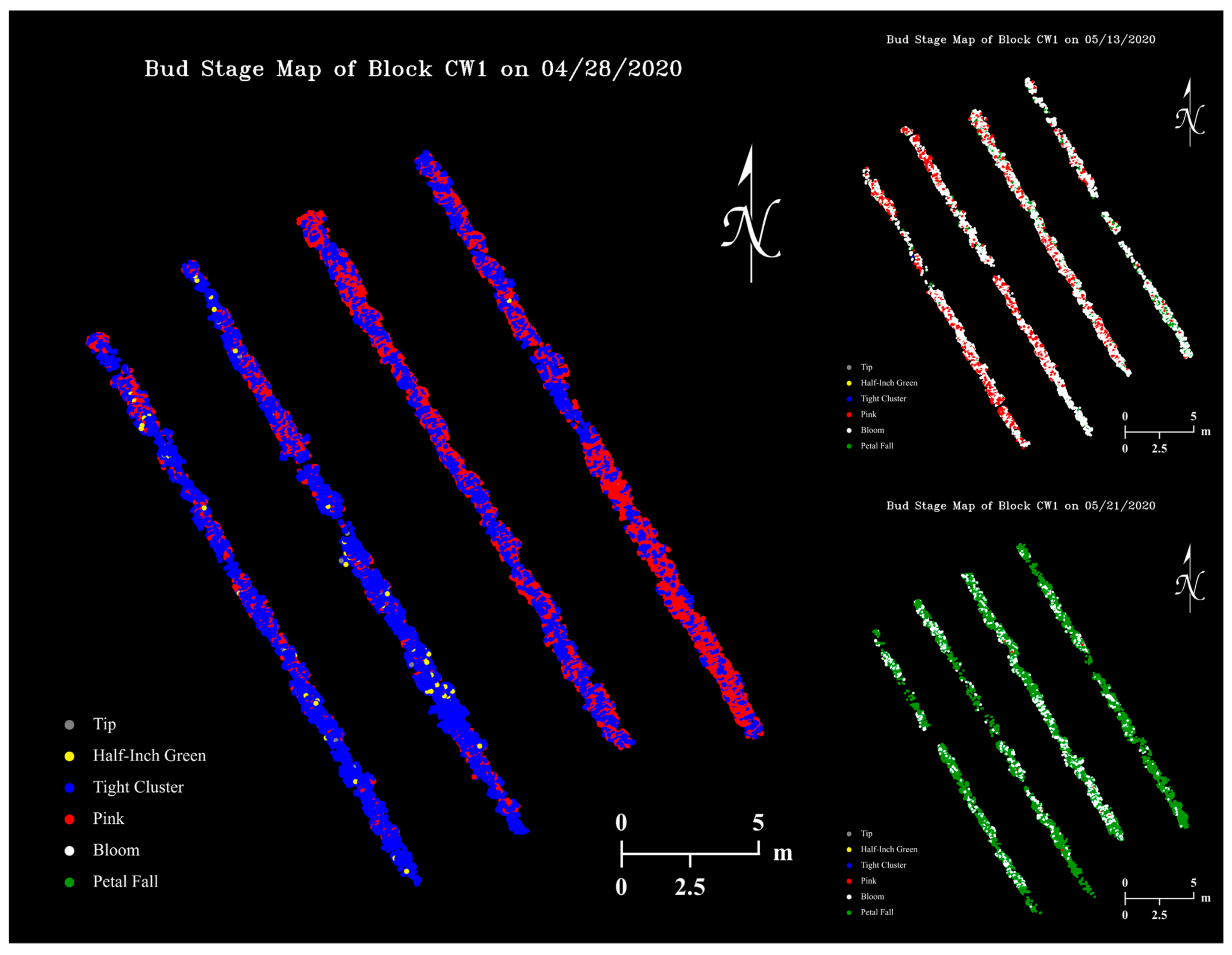
Using our Python program that applies a YOLOv4 classifier on RGB images and saves detection results to files, the size 480 classifier had an average image “inference time” of 0.16 s, while mapping detected buds to a thermal coordinate map had a negligible time cost. Figure 13 shows examples of apple flower bud growth stage maps generated with the size 480 classifier, where dots with different colors represent flower buds at various growth stages.
UAV GPS accuracy is a major factor for the success of apple flower bud mapping. When a bud appears in multiple images taken without optimal GPS signals, it is likely to be mapped multiple times as a bud cluster on the map. This is generally not an issue for determining orchard regional heating requirement as little to no temperature variation exists for tree thermal pixels with short distances in between. With navigation techniques such as real-time kinematic (RTK) [90], it is possible to achieve centimeter-level accuracy for UAV positioning.
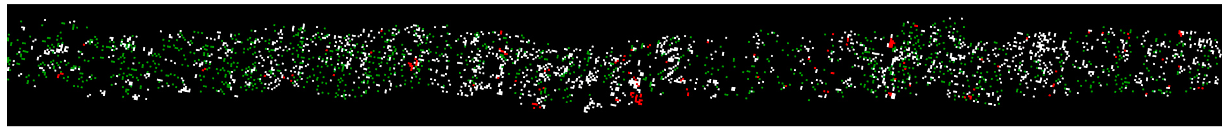
Unexpectedly, the flower bud growth stage maps seemed to have the potential to be an informative tool for agronomists to visualize both spatial variation (on the same map) and temporal changes (among different maps) of apple tree developments in high resolution (Figure 14). Potentially, growth stage timing and duration of different apple varieties could be studied when RGB datasets collected at shorter time intervals are available. In this study, most RGB images only sampled buds growing in the upper and center parts of tree canopies. The camera was not able to include lateral buds in a frame due to its limited FOV, while bottom buds were largely blocked by tree branches, leaves, and upper buds.
4.5. Orchard Heating Requirement Map
Using a temperature map from 2 June 2020 (Figure 11) and the flower bud growth stage map on 28 April 2020 (Figure 13), orchard heating requirement maps (Figure 15) were simulated assuming the critical temperatures of apple flower buds were 22, 19, and 18 °C higher than the actual values (Table 2). As can be observed in the maps, pixels with brighter colors represent orchard regions with higher heating demands, and sections of tree rows will disappear when it does not have any heating needs. The realization of map appearance in Figure 15 involved several image processing techniques including dilation, Gaussian blurring, and masking. Orchard heating requirement resolution can be increased by dilating pixels with smaller kernels, although practically lower resolution maps would be more suitable for determining regional heating treatments. Upon further dilations, the tree rows can be merged into an area, and heating requirement levels can be quantized to display discrete heating demand levels of the entire orchard.
5. Implications and Future Work
This article provides a framework for the concept of assisting orchard frost management with modern technologies and computer vision algorithms, for the purpose of minimizing labor and heating costs and maximizing management efficiency. However, any component of this framework can be modified as needed, although the outcome might be less optimal. For example, the UAV can be replaced with an unmanned ground vehicle, the YOLOv4 detector can be switched to other older but more widely implemented algorithms such as Faster R-CNN, and the image stitching can be completed using readily available commercial software.
From the application standpoint, our methodology requires flower bud growth stage maps to be obtained prior to temperature maps. As capturing high-quality RGB images requires good lighting conditions, without artificial lighting, RGB flight missions should only be conducted after sunrise and before sunset. Thermal flight missions, on the other hand, are not restricted by the time of day as objects emit infrared radiations at all times. In the daytime before a forecasted frost event, orchardists can either fly manually to sample buds at preplanned locations that are representative of the whole orchard, or set up autonomous flight missions to capture bud images as we demonstrated in this article, and then generate a flower bud growth stage map from the collected data using a pre-trained classifier. Note RGB image collection and flower bud growth stage map generation are not time-sensitive, unlike temperature map generation. Based on the assumption that there will be no significant flower bud growth stage changes overnight or within a day, during a frost event, orchardists can initiate a thermal flight mission whenever orchard temperatures need to be gauged. Depending on UAV flight altitudes and speeds, temperature maps can be created either in low resolution but quickly, or in high resolution but with a longer delay, and heating requirement maps can be generated as soon as the temperature maps are available. While a temperature map already allows orchardists to decide the level of needed heating treatments, a heating requirement map puts plant growth stage variation in an orchard in consideration to minimize unnecessary regional heating. Note that, depending on orchardists’ unique situations during frost events such as frost protection methods, orchard layout and topography, and weather conditions, plant temperatures can change at different rates, and orchard heating requirement maps might need to be generated at higher or lower frequencies for either timely orchard heating demand assessment or observable plant temperature changes.
Aside from orchard heaters, our proposed methodology can also be beneficial to other traditional frost protection methods such as irrigation. Although overhead or under-tree irrigation has disadvantages such as high installation cost, large water consumption, and causing broken branches due to ice overloading, it generally can protect trees from frost effectively through the heat of solidification of water. Unlike orchard thermometers that measure air temperatures, thermal cameras can directly assess how irrigation changes plant temperatures. With the information on a heating requirement map, variable rate irrigation (VRI) systems can potentially apply larger amounts of water to orchard regions with higher heating demands. On the other hand, large-scale frost management methods such as wind machine might not be the best match to our methodology. Wind machines increase orchard temperature simply by bringing warm air down from an inversion layer to ground level to break thermal stratification, and they typically have low operational costs. Yet, wind machines do not work under cold, windy conditions, and they cannot make the most use of a heating requirement map with localized orchard heating demands as a single commercial wind machine often covers an area up to 40,000 to 60,000 m2. The methodology of orchard heating requirement determination proposed in this article does not come without limitations. Weather condition is a major factor that influences UAV performance in the air. Using DJI Matrice 600 Pro as an example, it cannot be operated in rain or snow as it is not a waterproof drone, and it has a lower operating temperature limit of −10 °C and a maximum wind resistance of 8 m/s. In addition to affecting drone stability, strong wind can also significantly reduce image quality by causing tree movements. For large orchards, multiple sets of batteries might be needed for prolonged flight missions. As thermal cameras have limited dynamic ranges, with the presence of heating sources such as orchard heaters, thermal cameras can be blinded and fail to prevent overheating in the heating region. Before trees develop leaves, it can be challenging to map detected flower buds such as tips exactly onto tree branch pixels of a temperature map, as doing so requires navigation systems with very high precision. Luckily, during such growth stages flower buds also tend to have high cold resistance [12] and frost damage is not a prominent issue. The total cost of equipment used in this study, including a UAV, a thermal camera, an RGB camera, an iPad, two extra sets of UAV batteries, and a computer, was up to $25,000. Despite being a big initial investment, this amount could be substantially cheaper when compared to human labor costs for temperature monitoring of large orchards in the long-term.
To fully automate orchard frost management, future studies should focus on the development of heating platforms that are capable of site-specific heating such as self-navigating heating mobiles, as well as the communication and systemic integration of temperature monitoring devices and heating units. For example, a cyberphysical system consisting of UAV-based orchard heating requirement assessment, unmanned ground vehicle (UGV)-based heating, and station-based vehicle communication, UAV data processing, and heating treatment determination has the potential to replace current manual frost protection methods. A UAV can maintain a predefined search pattern to monitor orchard temperatures, while a UGV will be dispatched to apply heating treatments as soon as orchard temperatures fall below the critical levels. A orchard heating requirement map generated by a base station using our proposed methodology contains both temperature and location information, which can be further utilized by the base station to decide the order of heating locations and the duration of heating treatments for the UGV. With the advancements of modern object detection algorithms such as YOLOv4, real-time heating demand determination is possible by flying thermal and RGB cameras simultaneously, applying flower bud detector on RGB data, and registering thermal and RGB video frames, although much hardware integration and software development need to be involved to achieve robust results.
6. Conclusions
In this article, the concept of utilizing a UAV-based thermal camera for temperature monitoring and an RGB camera for plant growth stage spatial variability characterization in apple orchard was demonstrated. The thermal image stitching algorithm produced georeferenced temperature maps with high resolutions sufficient for individual flower bud mapping, whose generation time can be improved by sacrificing thermal mosaic resolutions for more timely orchard temperature assessments. The fully functioning YOLOv4 apple flower bud growth stage classifier achieved satisfactory performance considering the difficulty of the RGB datasets. Training the classifier with new images or larger image input sizes might improve APs of certain growth stages, while refining existing image labels is more likely to fundamentally enhance the model sophistication. Orchard heating demand variations were observed in the simulated heating requirement maps, which proved uniform heating treatments for frost protection in orchards might be wasteful. We conclude our proposed methodology of orchard heating requirements determination is feasible, and this study can serve as a stepping stone for future research on fully autonomous, site-specific orchard frost management systems.
Author Contributions
Conceptualization, D.C.; methodology, W.Y. and D.C.; software, W.Y.; validation, W.Y.; formal analysis, W.Y.; investigation, W.Y.; resources, D.C.; data curation, W.Y.; writing—original draft preparation, W.Y.; writing—review and editing, W.Y. and D.C.; visualization, W.Y.; supervision, D.C.; project administration, D.C.; funding acquisition, D.C. All authors have read and agreed to the published version of the manuscript.
Funding
This work was supported by the National Science Foundation, the USDA National Institute of Food and Agriculture under Accession #1018998 and Award #2019–67021-29224, the USDA National Institute of Food and Agriculture Multistate Research under Project #PEN04653 and Accession #1016510.
Data Availability Statement
The data presented in this study are available on request from the corresponding author.
Acknowledgments
The authors would like to thank Donald Edwin Smith for providing the background information of the apple orchard; Omeed Mirbod for the help on measuring GCPs’ GPS coordinates; and Valerie Alexandra Godoy, Satoshi Sueyoshi, Alexandra Luna, and Samuel Anderson for the help on image labeling.
Conflicts of Interest
The authors declare no conflict of interest.
References
- Moeletsi, M.E.; Tongwane, M.I. Spatiotemporal variation of frost within growing periods. Adv. Meteorol. 2017, 2017, 1–11. [Google Scholar] [CrossRef] [Green Version]
- Papagiannaki, K.; Lagouvardos, K.; Kotroni, V.; Papagiannakis, G. Agricultural losses related to frost events: Use of the 850 hPa level temperature as an explanatory variable of the damage cost. Nat. Hazards Earth Syst. Sci. 2014, 14, 2375–2386. [Google Scholar] [CrossRef] [Green Version]
- Perry, K.B. Basics of frost and freeze protection for horticultural crops. Horttechnology 1998, 8, 10–15. [Google Scholar] [CrossRef] [Green Version]
- Savage, M.J. Estimation of frost occurrence and duration of frost for a short-grass surface. S. Afr. J. Plant. Soil 2012, 29, 173–181. [Google Scholar] [CrossRef]
- Snyder, R.L.; de Melo-Abreu, J.P. Frost Protection: Fundamentals, Practice, and Economics; Food and Agriculture Organization (FAO): Rome, Italy, 2005; Volume 1, ISBN 92-5-105328-6. [Google Scholar]
- Yue, Y.; Zhou, Y.; Wang, J.; Ye, X. Assessing wheat frost risk with the support of GIS: An approach coupling a growing season meteorological index and a hybrid fuzzy neural network model. Sustainability 2016, 8, 1308. [Google Scholar] [CrossRef] [Green Version]
- Pearce, R.S. Plant freezing and damage. Ann. Bot. 2001, 87, 417–424. [Google Scholar] [CrossRef]
- Lindow, S.E. The role of bacterial ice nucleation in frost injury to plants. Annu. Rev. Phytopathol. 1983, 21, 363–384. [Google Scholar] [CrossRef]
- Teitel, M.; Peiper, U.M.; Zvieli, Y. Shading screens for frost protection. Agric. For. Meteorol. 1996, 81, 273–286. [Google Scholar] [CrossRef]
- Eccel, E.; Rea, R.; Caffarra, A.; Crisci, A. Risk of spring frost to apple production under future climate scenarios: The role of phenological acclimation. Int. J. Biometeorol. 2009, 53, 273–286. [Google Scholar] [CrossRef]
- Ribeiro, A.C.; de Melo-Abreu, J.P.; Snyder, R.L. Apple orchard frost protection with wind machine operation. Agric. Forest Meteorol. 2006, 141, 71–81. [Google Scholar] [CrossRef]
- Ballard, J.K.; Proebsting, E.L. Frost and Frost Control in Washington Orchards; Washington State University Extension: Pullman, WA, USA, 1972. [Google Scholar]
- Cisternas, I.; Velásquez, I.; Caro, A.; Rodríguez, A. Systematic literature review of implementations of precision agriculture. Comput. Electron. Agric. 2020, 176, 105626. [Google Scholar] [CrossRef]
- Tsouros, D.C.; Bibi, S.; Sarigiannidis, P.G. A review on UAV-based applications for precision agriculture. Information 2019, 10, 349. [Google Scholar] [CrossRef] [Green Version]
- Tsouros, D.C.; Triantafyllou, A.; Bibi, S.; Sarigannidis, P.G. Data acquisition and analysis methods in UAV- based applications for precision agriculture. In Proceedings of the 2019 15th International Conference on Distributed Computing in Sensor Systems (DCOSS), Santorini Island, Greece, 29–31 May 2019; pp. 377–384. [Google Scholar]
- Zarco-Tejada, P.J.; González-Dugo, V.; Berni, J.A.J. Fluorescence, temperature and narrow-band indices acquired from a UAV platform for water stress detection using a micro-hyperspectral imager and a thermal camera. Remote Sens. Environ. 2012, 117, 322–337. [Google Scholar] [CrossRef]
- Santesteban, L.G.; Di Gennaro, S.F.; Herrero-Langreo, A.; Miranda, C.; Royo, J.B.; Matese, A. High-resolution UAV-based thermal imaging to estimate the instantaneous and seasonal variability of plant water status within a vineyard. Agric. Water Manag. 2017, 183, 49–59. [Google Scholar] [CrossRef]
- Matese, A.; Di Gennaro, S.F. Practical applications of a multisensor UAV platform based on multispectral, thermal and RGB high resolution images in precision viticulture. Agriculture 2018, 8, 116. [Google Scholar] [CrossRef] [Green Version]
- García-Tejero, I.F.; Ortega-Arévalo, C.J.; Iglesias-Contreras, M.; Moreno, J.M.; Souza, L.; Tavira, S.C.; Durán-Zuazo, V.H. Assessing the crop-water status in almond (Prunus dulcis Mill.) trees via thermal imaging camera connected to smartphone. Sensors 2018, 18, 1050. [Google Scholar]
- Zhang, L.; Niu, Y.; Zhang, H.; Han, W.; Li, G.; Tang, J.; Peng, X. Maize canopy temperature extracted from UAV thermal and RGB imagery and its application in water stress monitoring. Front. Plant. Sci. 2019, 10, 1270. [Google Scholar] [CrossRef]
- Crusiol, L.G.T.; Nanni, M.R.; Furlanetto, R.H.; Sibaldelli, R.N.R.; Cezar, E.; Mertz-Henning, L.M.; Nepomuceno, A.L.; Neumaier, N.; Farias, J.R.B. UAV-based thermal imaging in the assessment of water status of soybean plants. Int. J. Remote Sens. 2020, 41, 3243–3265. [Google Scholar] [CrossRef]
- Quebrajo, L.; Perez-Ruiz, M.; Pérez-Urrestarazu, L.; Martínez, G.; Egea, G. Linking thermal imaging and soil remote sensing to enhance irrigation management of sugar beet. Biosyst. Eng. 2018, 165, 77–87. [Google Scholar] [CrossRef]
- Ezenne, G.I.; Jupp, L.; Mantel, S.K.; Tanner, J.L. Current and potential capabilities of UAS for crop water productivity in precision agriculture. Agric. Water Manag. 2019, 218, 158–164. [Google Scholar] [CrossRef]
- Liu, T.; Li, R.; Zhong, X.; Jiang, M.; Jin, X.; Zhou, P.; Liu, S.; Sun, C.; Guo, W. Estimates of rice lodging using indices derived from UAV visible and thermal infrared images. Agric. Forest Meteorol. 2018, 252, 144–154. [Google Scholar] [CrossRef]
- Sankaran, S.; Quirós, J.J.; Miklas, P.N. Unmanned aerial system and satellite-based high resolution imagery for high-throughput phenotyping in dry bean. Comput. Electron. Agric. 2019, 165, 104965. [Google Scholar] [CrossRef]
- Zhou, J.; Khot, L.R.; Boydston, R.A.; Miklas, P.N.; Porter, L. Low altitude remote sensing technologies for crop stress monitoring: A case study on spatial and temporal monitoring of irrigated pinto bean. Precis. Agric. 2018, 19, 555–569. [Google Scholar] [CrossRef]
- Ren, P.; Meng, Q.; Zhang, Y.; Zhao, L.; Yuan, X.; Feng, X. An unmanned airship thermal infrared remote sensing system for low-altitude and high spatial resolution monitoring of urban thermal environments: Integration and an experiment. Remote Sens. 2015, 7, 14259–14275. [Google Scholar] [CrossRef] [Green Version]
- Quaritsch, M.; Kruggl, K.; Wischounig-Strucl, D.; Bhattacharya, S.; Shah, M.; Rinner, B. Networked UAVs as aerial sensor network for disaster management applications. Elektrotechnik und Informationstechnik 2010, 127, 56–63. [Google Scholar] [CrossRef]
- Brown, M.; Lowe, D.G. Automatic panoramic image stitching using invariant features. Int. J. Comput. Vis. 2007, 74, 59–73. [Google Scholar] [CrossRef] [Green Version]
- Girshick, R.; Donahue, J.; Darrell, T.; Malik, J. Rich feature hierarchies for accurate object detection and semantic segmentation. In Proceedings of the 2014 IEEE Conference on Computer Vision and Pattern Recognition, Columbus, OH, USA, 23–28 June 2014; pp. 580–587. [Google Scholar]
- Girshick, R. Fast R-CNN. In Proceedings of the 2015 IEEE International Conference on Computer Vision (ICCV), Santiago, Chile, 7–15 December 2015; pp. 1440–1448. [Google Scholar]
- Ren, S.; He, K.; Girshick, R.; Sun, J. Faster R-CNN: Towards real-time object detection with region proposal networks. IEEE Trans. Pattern Anal. Mach. Intell. 2017, 39, 1137–1149. [Google Scholar] [CrossRef] [Green Version]
- He, K.; Gkioxari, G.; Dollár, P.; Girshick, R. Mask R-CNN. In Proceedings of the 2017 IEEE International Conference on Computer Vision (ICCV), Venice, Italy, 22–29 October 2017; pp. 2980–2988. [Google Scholar]
- Pang, J.; Chen, K.; Shi, J.; Feng, H.; Ouyang, W.; Lin, D. Libra R-CNN: Towards balanced learning for object detection. In Proceedings of the 2019 IEEE/CVF Conference on Computer Vision and Pattern Recognition (CVPR), Long Beach, CA, USA, 16–20 June 2019; pp. 821–830. [Google Scholar]
- Redmon, J.; Divvala, S.; Girshick, R.; Farhadi, A. You only look once: Unified, real-time object detection. In Proceedings of the 2016 IEEE Conference on Computer Vision and Pattern Recognition (CVPR), Las Vegas, NV, USA, 27–30 June 2016; pp. 779–788. [Google Scholar]
- Redmon, J.; Farhadi, A. YOLO9000: Better, faster, stronger. In Proceedings of the 2017 IEEE Conference on Computer Vision and Pattern Recognition (CVPR), Honolulu, HI, USA, 21–26 July 2017; pp. 6517–6525. [Google Scholar]
- Redmon, J.; Farhadi, A. YOLOv3: An incremental improvement. arXiv 2018, arXiv:1804.02767. [Google Scholar]
- Bochkovskiy, A.; Wang, C.-Y.; Liao, H.-Y.M. YOLOv4: Optimal speed and accuracy of object detection. arXiv 2020, arXiv:2004.10934. [Google Scholar]
- Grimm, J.; Herzog, K.; Rist, F.; Kicherer, A.; Töpfer, R.; Steinhage, V. An adaptable approach to automated visual detection of plant organs with applications in grapevine breeding. Biosyst. Eng. 2019, 183, 170–183. [Google Scholar] [CrossRef]
- Chen, Y.; Lee, W.S.; Gan, H.; Peres, N.; Fraisse, C.; Zhang, Y.; He, Y. Strawberry yield prediction based on a deep neural network using high-resolution aerial orthoimages. Remote Sens. 2019, 11, 1584. [Google Scholar] [CrossRef] [Green Version]
- Koirala, A.; Walsh, K.B.; Wang, Z.; Anderson, N. Deep learning for mango (Mangifera indica) panicle stage classification. Agronomy 2020, 10, 143. [Google Scholar] [CrossRef] [Green Version]
- Milicevic, M.; Zubrinic, K.; Grbavac, I.; Obradovic, I. Application of deep learning architectures for accurate detection of olive tree flowering phenophase. Remote Sens. 2020, 12, 2120. [Google Scholar] [CrossRef]
- Ärje, J.; Milioris, D.; Tran, D.T.; Jepsen, J.U.; Raitoharju, J.; Gabbouj, M.; Iosifidis, A.; Høye, T.T. Automatic flower detection and classification system using a light-weight convolutional neural network. In Proceedings of the EUSIPCO Workshop on Signal Processing, Computer Vision and Deep Learning for Autonomous Systems, A Coruña, Spain, 2–6 September 2019. [Google Scholar]
- Davis, C.C.; Champ, J.; Park, D.S.; Breckheimer, I.; Lyra, G.M.; Xie, J.; Joly, A.; Tarapore, D.; Ellison, A.M.; Bonnet, P. A new method for counting reproductive structures in digitized herbarium specimens using Mask R-CNN. Front. Plant. Sci. 2020, 11, 1129. [Google Scholar] [CrossRef] [PubMed]
- Ponn, T.; Kröger, T.; Diermeyer, F. Identification and explanation of challenging conditions for camera-based object detection of automated vehicles. Sensors 2020, 20, 3699. [Google Scholar] [CrossRef]
- Helala, M.A.; Zarrabeitia, L.A.; Qureshi, F.Z. Mosaic of near ground UAV videos under parallax effects. In Proceedings of the 6th International Conference on Distributed Smart Cameras (ICDSC), Hong Kong, China, 30 October–2 November 2012; pp. 1–6. [Google Scholar]
- Feng, L.; Tian, H.; Qiao, Z.; Zhao, M.; Liu, Y. Detailed variations in urban surface temperatures exploration based on unmanned aerial vehicle thermography. IEEE J. Sel. Top. Appl. Earth Obs. Remote Sens. 2019, 13, 204–216. [Google Scholar] [CrossRef]
- Sagan, V.; Maimaitijiang, M.; Sidike, P.; Eblimit, K.; Peterson, K.T.; Hartling, S.; Esposito, F.; Khanal, K.; Newcomb, M.; Pauli, D.; et al. UAV-based high resolution thermal imaging for vegetation monitoring, and plant phenotyping using ICI 8640 P, FLIR Vue Pro R 640, and thermomap cameras. Remote Sens. 2019, 11, 330. [Google Scholar] [CrossRef] [Green Version]
- Osroosh, Y.; Peters, R.T.; Campbell, C.S. Estimating actual transpiration of apple trees based on infrared thermometry. J. Irrig. Drain. Eng. 2015, 141, 1–13. [Google Scholar] [CrossRef]
- Masuda, K.; Takashima, T.; Takayama, Y. Emissivity of pure and sea waters for the model sea surface in the infrared window regions. Remote Sens. Environ. 1988, 24, 313–329. [Google Scholar] [CrossRef]
- Wang, Y.; Camargo, A.; Fevig, R.; Martel, F.; Schultz, R.R. Image mosaicking from uncooled thermal IR video captured by a small UAV. In Proceedings of the 2008 IEEE Southwest Symposium on Image Analysis and Interpretation, Santa Fe, NM, USA, 24–26 March 2008; pp. 161–164. [Google Scholar]
- Lowe, D.G. Object recognition from local scale-invariant features. In Proceedings of the Seventh IEEE International Conference on Computer Vision, Kerkyra, Greece, 20–27 September 1999; pp. 1150–1157. [Google Scholar]
- Bay, H.; Tuytelaars, T.; Van Gool, L. SURF: Speeded up robust features. In Proceedings of the 9th European Conference on Computer Vision (ECCV 2006), Graz, Austria, 7–13 May 2006; pp. 404–417. [Google Scholar]
- Leutenegger, S.; Chli, M.; Siegwart, R.Y. BRISK: Binary robust invariant scalable keypoints. In Proceedings of the 2011 International Conference on Computer Vision, Barcelona, Spain, 6–13 November 2011; pp. 2548–2555. [Google Scholar]
- Rosten, E.; Drummond, T. Machine learning for high-speed corner detection. In Proceedings of the 9th European Conference on Computer Vision (ECCV 2006), Graz, Austria, 7–13 May 2006; pp. 430–443. [Google Scholar]
- Tareen, S.A.K.; Saleem, Z. A comparative analysis of SIFT, SURF, KAZE, AKAZE, ORB, and BRISK. In Proceedings of the 2018 International Conference on Computing, Mathematics and Engineering Technologies (iCoMET), Sukkur, Pakistan, 3–4 March 2018; pp. 1–10. [Google Scholar]
- OpenCV. Available online: https://opencv.org/ (accessed on 25 October 2020).
- Scikit-Image. Available online: https://scikit-image.org/ (accessed on 25 October 2020).
- Hamming, R.W. Error detecting and error correcting codes. Bell Syst. Tech. J. 1950, 29, 147–160. [Google Scholar] [CrossRef]
- Lowe, D.G. Distinctive image features from scale-invariant keypoints. Int. J. Comput. Vis. 2004, 60, 91–110. [Google Scholar] [CrossRef]
- Fischler, M.A.; Bolles, R.C. Random sample consensus: A paradigm for model fitting with applications to image analysis and automated cartography. Commun. ACM 1981, 24, 381–395. [Google Scholar] [CrossRef]
- Yuen, H.K.; Princen, J.; Illingworth, J.; Kittler, J. Comparative study of Hough Transform methods for circle finding. Image Vis. Comput. 1990, 8, 71–77. [Google Scholar] [CrossRef] [Green Version]
- Ballard, J.K.; Proebsting, E.L.; Tukey, R.B. Apples: Critical Temperatures for Blossom Buds; Washington State University Extension: Pullman, WA, USA, 1971. [Google Scholar]
- Meier, U.; Graf, M.; Hess, W.; Kennel, W.; Klose, R.; Mappes, D.; Seipp, D.; Stauss, R.; Streif, J.; van den Boom, T. Phänologische entwicklungsstadien des kernobstes (Malus domestica Borkh. und Pyrus communis L.), des steinobstes (Prunus-Arten), der Johannisbeere (Ribes-Arten) und der erdbeere (Fragaria x ananassa Duch.). Nachrichten Blatt des Deutschen Pflanzenschutzdienstes 1994, 46, 141–153. [Google Scholar]
- Koutinas, N.; Pepelyankov, G.; Lichev, V. Flower induction and flower bud development in apple and sweet cherry. Biotechnol. Biotechnol. Equip. 2010, 24, 1549–1558. [Google Scholar] [CrossRef]
- Lin, T.-Y.; Maire, M.; Belongie, S.; Bourdev, L.; Girshick, R.; Hays, J.; Perona, P.; Ramanan, D.; Zitnick, C.L.; Dollár, P. Microsoft COCO: Common objects in context. In Proceedings of the 13th European Conference on Computer Vision (ECCV), Zurich, Switzerland, 6–12 September 2014; pp. 740–755. [Google Scholar]
- Wang, C.-Y.; Liao, H.-Y.M.; Yeh, I.-H.; Wu, Y.-H.; Chen, P.-Y.; Hsieh, J.-W. CSPNet: A New Backbone that can Enhance Learning Capability of CNN. arXiv 2019, arXiv:1911.11929. [Google Scholar]
- Misra, D. Mish: A self regularized non-monotonic neural activation function. arXiv 2019, arXiv:1908.08681. [Google Scholar]
- He, K.; Zhang, X.; Ren, S.; Sun, J. Spatial pyramid pooling in deep convolutional networks for visual recognition. IEEE Trans. Pattern Anal. Mach. Intell. 2015, 37, 1904–1916. [Google Scholar] [CrossRef] [PubMed] [Green Version]
- Liu, S.; Qi, L.; Qin, H.; Shi, J.; Jia, J. Path aggregation network for instance segmentation. In Proceedings of the 2018 IEEE/CVF Conference on Computer Vision and Pattern Recognition, Salt Lake City, UT, USA, 18–23 June 2018; pp. 8759–8768. [Google Scholar]
- Yolo_Label. Available online: https://github.com/developer0hye/Yolo_Label (accessed on 30 September 2020).
- Everingham, M.; Van Gool, L.; Williams, C.K.I.; Winn, J.; Zisserman, A. The pascal visual object classes (VOC) challenge. Int. J. Comput. Vis. 2010, 88, 303–338. [Google Scholar] [CrossRef] [Green Version]
- Veness, C. Calculate Distance, Bearing and More between Latitude/Longitude Points. Available online: https://www.movable-type.co.uk/scripts/latlong.html (accessed on 5 October 2020).
- Han, X.; Thomasson, J.A.; Siegfried, J.; Raman, R.; Rajan, N.; Neely, H. Calibrating UAV-based thermal remote-sensing images of crops with temperature controlled references. In Proceedings of the 2019 ASABE Annual International Meeting, Boston, MA, USA, 7–10 July 2019; p. 1900662. [Google Scholar]
- Harvey, M.C.; Hare, D.K.; Hackman, A.; Davenport, G.; Haynes, A.B.; Helton, A.; Lane, J.W.; Briggs, M.A. Evaluation of stream and wetland restoration using UAS-based thermal infrared mapping. Water 2019, 11, 1568. [Google Scholar] [CrossRef] [Green Version]
- Collas, F.P.L.; van Iersel, W.K.; Straatsma, M.W.; Buijse, A.D.; Leuven, R.S.E.W. Sub-daily temperature heterogeneity in a side channel and the influence on habitat suitability of freshwater fish. Remote Sens. 2019, 11, 2367. [Google Scholar] [CrossRef] [Green Version]
- Deane, S.; Avdelidis, N.P.; Ibarra-Castanedo, C.; Zhang, H.; Nezhad, H.Y.; Williamson, A.A.; Mackley, T.; Maldague, X.; Tsourdos, A.; Nooralishahi, P. Comparison of cooled and uncooled IR sensors by means of signal-to-noise ratio for NDT diagnostics of aerospace grade composites. Sensors 2020, 20, 3381. [Google Scholar] [CrossRef] [PubMed]
- Torres-Rua, A. Vicarious calibration of sUAS microbolometer temperature imagery for estimation of radiometric land surface temperature. Sensors 2017, 17, 1499. [Google Scholar] [CrossRef] [PubMed] [Green Version]
- Zhao, T.; Niu, H.; Anderson, A.; Chen, Y.; Viers, J. A detailed study on accuracy of uncooled thermal cameras by exploring the data collection workflow. In Proceedings of the Autonomous Air and Ground Sensing Systems for Agricultural Optimization and Phenotyping III, Orlando, FL, USA, 18–19 April 2018; p. 106640F. [Google Scholar]
- Berni, J.A.J.; Zarco-Tejada, P.J.; Suárez, L.; Fereres, E. Thermal and narrowband multispectral remote sensing for vegetation monitoring from an unmanned aerial vehicle. IEEE Trans. Geosci. Remote Sens. 2009, 47, 722–738. [Google Scholar] [CrossRef] [Green Version]
- Aubrecht, D.M.; Helliker, B.R.; Goulden, M.L.; Roberts, D.A.; Still, C.J.; Richardson, A.D. Continuous, long-term, high-frequency thermal imaging of vegetation: Uncertainties and recommended best practices. Agric. Forest Meteorol. 2016, 228–229, 315–326. [Google Scholar] [CrossRef] [Green Version]
- Teza, G. THIMRAN: MATLAB toolbox for thermal image processing aimed at damage recognition in large bodies. J. Comput. Civ. Eng. 2014, 28, 04014017. [Google Scholar] [CrossRef]
- Sartinas, E.G.; Psarakis, E.Z.; Lamprinou, N. UAV forest monitoring in case of fire: Robustifying video stitching by the joint use of optical and thermal cameras. In Advances in Service and Industrial Robotics: Proceedings of the 27th International Conference on Robotics in Alpe-Adria-Danube Region (RAAD 2018); Springer: Cham, Switzerland, 2019; pp. 163–172. [Google Scholar]
- Evangelidis, G.D.; Psarakis, E.Z. Parametric image alignment using enhanced correlation coefficient maximization. IEEE Trans. Pattern Anal. Mach. Intell. 2008, 30, 1858–1865. [Google Scholar] [CrossRef] [Green Version]
- Semenishchev, E.; Agaian, S.; Voronin, V.; Pismenskova, M.; Zelensky, A.; Tolstova, I. Thermal image stitching for examination industrial buildings. In Proceedings of the Mobile Multimedia/Image Processing, Security, and Applications 2019, Baltimore, MD, USA, 15 April 2019; p. 109930M. [Google Scholar]
- Semenishchev, E.; Voronin, V.; Zelensky, A.; Shraifel, I. Algorithm for image stitching in the infrared. In Proceedings of the Infrared Technology and Applications XLV, Baltimore, MD, USA, 14–18 April 2019; p. 110022H. [Google Scholar]
- Yahyanejad, S.; Misiorny, J.; Rinner, B. Lens distortion correction for thermal cameras to improve aerial imaging with small-scale UAVs. In Proceedings of the 2011 IEEE International Symposium on Robotic and Sensors Environments (ROSE), Montreal, QC, USA, 17–18 September 2011; pp. 231–236. [Google Scholar]
- Tian, Y.; Yang, G.; Wang, Z.; Li, E.; Liang, Z. Instance segmentation of apple flowers using the improved mask R–CNN model. Biosyst. Eng. 2020, 193, 264–278. [Google Scholar] [CrossRef]
- Wu, D.; Lv, S.; Jiang, M.; Song, H. Using channel pruning-based YOLO v4 deep learning algorithm for the real-time and accurate detection of apple flowers in natural environments. Comput. Electron. Agric. 2020, 178, 105742. [Google Scholar] [CrossRef]
- Sun, H.; Slaughter, D.C.; Ruiz, M.P.; Gliever, C.; Upadhyaya, S.K.; Smith, R.F. RTK GPS mapping of transplanted row crops. Comput. Electron. Agric. 2010, 71, 32–37. [Google Scholar] [CrossRef]
Figure 1.
Hardware components employed in the study: (a) unmanned aerial vehicle (UAV), (b) thermal camera, and (c) red green blue (RGB) camera.
Figure 1.
Hardware components employed in the study: (a) unmanned aerial vehicle (UAV), (b) thermal camera, and (c) red green blue (RGB) camera.

Figure 2.
Flight path of the thermal and RGB flight missions conducted over the apple orchard (Russell E. Larson Agricultural Research Center, Pennsylvania Furnace, PA, USA).
Figure 2.
Flight path of the thermal and RGB flight missions conducted over the apple orchard (Russell E. Larson Agricultural Research Center, Pennsylvania Furnace, PA, USA).

Figure 3.
Illustration of the thermal camera calibration: (a) temperature measurement of the thermal camera calibration target with a digital thermometer; (b,c) example thermal images containing the calibration target before cropping taken at 10 °C and 75 °C water temperatures.
Figure 3.
Illustration of the thermal camera calibration: (a) temperature measurement of the thermal camera calibration target with a digital thermometer; (b,c) example thermal images containing the calibration target before cropping taken at 10 °C and 75 °C water temperatures.

Figure 4.
An example of stitching two consecutive thermal images taken over the orchard showing a section of two rows of apple trees: (a) inliers of the matched BRISK keypoints between two images and (b) the stitching result.
Figure 4.
An example of stitching two consecutive thermal images taken over the orchard showing a section of two rows of apple trees: (a) inliers of the matched BRISK keypoints between two images and (b) the stitching result.

Figure 5.
A ground control point (GCP) for georeferencing thermal mosaics: (a) in the orchard, (b) its appearance in a thermal image, and (c) being detected by our algorithm.
Figure 5.
A ground control point (GCP) for georeferencing thermal mosaics: (a) in the orchard, (b) its appearance in a thermal image, and (c) being detected by our algorithm.

Figure 6.
Examples of apple flower bud annotations at various growth stages: (a) tip, (b) half-inch green, (c) tight cluster, (d,e) pink, (f) bloom, and (g,h) petal fall.
Figure 6.
Examples of apple flower bud annotations at various growth stages: (a) tip, (b) half-inch green, (c) tight cluster, (d,e) pink, (f) bloom, and (g,h) petal fall.

Figure 7.
Schematic diagram illustrating GPS coordinate calculation of a detected bud in an RGB image.
Figure 7.
Schematic diagram illustrating GPS coordinate calculation of a detected bud in an RGB image.

Figure 8.
A simplified heating requirement map containing three heating requirement pixels of three different apple flower buds, where brighter pixels represent higher heating demands: (a) before dilation and (b) buds with higher heating requirements are prioritized after dilation by overwriting small pixel values with larger pixel values in the overlapping area.

Figure 9.
Calibrated relationship between thermal pixel intensity and temperature based on least-squares regression.
Figure 9.
Calibrated relationship between thermal pixel intensity and temperature based on least-squares regression.

Figure 10.
Stitched thermal mosaic examples of the apple orchard under different weather conditions: (a) mostly sunny, (b) partially sunny, and (c) mostly cloudy.
Figure 10.
Stitched thermal mosaic examples of the apple orchard under different weather conditions: (a) mostly sunny, (b) partially sunny, and (c) mostly cloudy.

Figure 11.
Examples of grayscale and false-color apple orchard temperature maps generated from the same thermal mosaic.
Figure 11.
Examples of grayscale and false-color apple orchard temperature maps generated from the same thermal mosaic.

Figure 12.
Detection results of the size 480 classifier on sample apple flower bud RGB images with high bud distribution density.
Figure 12.
Detection results of the size 480 classifier on sample apple flower bud RGB images with high bud distribution density.

Figure 13.
Apple flower bud growth stage map examples of the apple orchard on three data collection dates generated with the size 480 classifier.
Figure 13.
Apple flower bud growth stage map examples of the apple orchard on three data collection dates generated with the size 480 classifier.

Figure 14.
A close-up view of the apple flower bud growth stage map on 16 May 2020, showing actual floral density of a tree row section with each detected flower bud mapped as one pixel.
Figure 14.
A close-up view of the apple flower bud growth stage map on 16 May 2020, showing actual floral density of a tree row section with each detected flower bud mapped as one pixel.

Figure 15.
Orchard heating requirement map examples simulated based on the 2 June 2020 temperature map and the 28 April 2020 flower bud growth stage map with three levels of artificial critical temperatures.
Figure 15.
Orchard heating requirement map examples simulated based on the 2 June 2020 temperature map and the 28 April 2020 flower bud growth stage map with three levels of artificial critical temperatures.


Table 1.
Key specifications of hardware components employed in the study.
| Hardware | Model | Specification |
|---|---|---|
| UAV | DJI Matrice 600 Pro (with TB47S batteries) | 6 kg payload, 16 to 32 min hovering time, ±0.5 m vertical and ±1.5 m horizontal hovering accuracy |
| Thermal camera | DJI Zenmuse XT2 (with a 19 mm lens) | −25 to 135 °C scene range, 7.5 to 13.5 µm spectral range, 32° × 26° FOV, 640 × 512 resolution |
| RGB camera | DJI Zenmuse Z30 | 30× optical zoom, 63.7° × 38.52° wide-end FOV, 2.3° × 1.29° tele-end FOV, 1920 × 1080 resolution |
Table 2.
Critical temperatures (10% kill) in Celsius of the six apple flower bud growth stages adopted in this study, which are defined as the temperatures that buds will endure for 30 minutes or less without injury [12].
Table 2.
Critical temperatures (10% kill) in Celsius of the six apple flower bud growth stages adopted in this study, which are defined as the temperatures that buds will endure for 30 minutes or less without injury [12].
| Growth Stage | Tip | Half-Inch Green | Tight Cluster | Pink | Bloom | Petal Fall |
|---|---|---|---|---|---|---|
| BBCH-identification code [64] | 01–09 | 10–11 | 15–19 | 51–59 | 60–67 | 69 |
| Critical temperature | −8.89 | −5.00 | −2.78 | −2.22 | −2.22 | −1.67 |
Table 3.
Performance of three apple flower bud growth stage classifiers with different network sizes at 50% intersection over union (IoU) on the validation and test datasets.
Table 3.
Performance of three apple flower bud growth stage classifiers with different network sizes at 50% intersection over union (IoU) on the validation and test datasets.
| Statistics | Network Size | ||||||
|---|---|---|---|---|---|---|---|
| 320 × 320 | 480 × 480 | 640 × 640 | |||||
| Validation | Test | Validation | Test | Validation | Test | ||
| AP | Tip | 31.74% | 51.65% | 48.34% | 65.72% | 50.08% | 61.72% |
| Half-inch green | 39.48% | 50.46% | 48.25% | 57.08% | 45.95% | 56.68% | |
| Tight cluster | 85.07% | 86.98% | 85.50% | 87.65% | 82.83% | 85.48% | |
| Pink | 71.41% | 69.29% | 72.83% | 71.79% | 71.50% | 70.18% | |
| Bloom | 81.54% | 81.33% | 84.58% | 84.52% | 84.12% | 83.49% | |
| Petal fall | 57.34% | 56.75% | 63.46% | 62.68% | 63.69% | 62.88% | |
| mAP | 61.09% | 66.08% | 67.16% | 71.57% | 66.36% | 70.07% | |
Publisher’s Note: MDPI stays neutral with regard to jurisdictional claims in published maps and institutional affiliations. |
© 2021 by the authors. Licensee MDPI, Basel, Switzerland. This article is an open access article distributed under the terms and conditions of the Creative Commons Attribution (CC BY) license (http://creativecommons.org/licenses/by/4.0/).
Share and Cite
MDPI and ACS Style
Yuan, W.; Choi, D. UAV-Based Heating Requirement Determination for Frost Management in Apple Orchard. Remote Sens. 2021, 13, 273. https://doi.org/10.3390/rs13020273
AMA Style
Yuan W, Choi D. UAV-Based Heating Requirement Determination for Frost Management in Apple Orchard. Remote Sensing. 2021; 13(2):273. https://doi.org/10.3390/rs13020273
Chicago/Turabian StyleYuan, Wenan, and Daeun Choi. 2021. "UAV-Based Heating Requirement Determination for Frost Management in Apple Orchard" Remote Sensing 13, no. 2: 273. https://doi.org/10.3390/rs13020273
Note that from the first issue of 2016, this journal uses article numbers instead of page numbers. See further details here.