Article

Multi-Image-Feature-Based Hierarchical Concrete Crack Identification Framework Using Optimized SVM Multi-Classifiers and D–S Fusion Algorithm for Bridge Structures

1
Centre for Infrastructure Engineering, Western Sydney University, Penrith, NSW 2751, Australia
2
School of Architecture, Building and Civil Engineering, Loughborough University, Loughborough LE11 3TU, UK
*
Author to whom correspondence should be addressed.
Remote Sens. 2021, 13(2), 240; https://doi.org/10.3390/rs13020240
Submission received: 3 December 2020 / Revised: 5 January 2021 / Accepted: 8 January 2021 / Published: 12 January 2021
(This article belongs to the Section Engineering Remote Sensing)

Abstract

:
Cracks in concrete can cause the degradation of stiffness, bearing capacity and durability of civil infrastructure. Hence, crack diagnosis is of great importance in concrete research. On the basis of multiple image features, this work presents a novel approach for crack identification of concrete structures. Firstly, the non-local means method is adopted to process the original image, which can effectively diminish the noise influence. Then, to extract the effective features sensitive to the crack, different filters are employed for crack edge detection, which are subsequently tackled by integral projection and principal component analysis (PCA) for optimal feature selection. Moreover, support vector machine (SVM) is used to design the classifiers for initial diagnosis of concrete surface based on extracted features. To raise the classification accuracy, enhanced salp swarm algorithm (ESSA) is applied to the SVM for meta-parameter optimization. The Dempster–Shafer (D–S) fusion algorithm is utilized to fuse the diagnostic results corresponding to different filters for decision making. Finally, to demonstrate the effectiveness of the proposed framework, a total of 1200 images are collected from a real concrete bridge including intact (without crack), longitudinal crack, transverse crack and oblique crack cases. The results validate the performance of proposed method with promising results of diagnosis accuracy as high as 96.25%.

1. Introduction

As the most commonly used construction material, concrete has been widely used in civil infrastructure, such as buildings, tunnels, dams, bridges, and wharfs. However, most of these structures are susceptible to damage due to the environmental factors including wind, seawater, fog, ice, etc. [1,2,3,4]. Among various concrete damage types, crack is a typical concrete damage which can remarkably influence the stress distribution of structural components and undermine the structural integrity. For the reinforced concrete structure, the crack can also result in the corrosion of steel reinforcement and cause concrete cancer, which further accelerates the crack development and growth. Accordingly, timely and accurate identification of significant cracks on the structure surface is of great importance for protecting civil infrastructure and avoiding unnecessary economic loss. The traditional crack inspection methods are not only labour intensive and time consuming, but also lack the assurance of accuracy and being real-time [5,6]. With rapid development of computer vision technology, using a mobile camera system or remotely piloted aircraft (RPA) to monitor civil infrastructure, combined with advanced image processing to extract useful geometrical features of crack from captured videos or images, is a more reliable and robust solution compared to other contact-based approaches such as ultrasonic [7,8,9]. Although the ultrasonic-based techniques may effectively detect the internal defect or crack of the structure, the installation of such a device on the structure in use is not as convenient as that of imaging methods based on controllable mobile camera system.
To effectively identify the concrete crack, a large number of studies have been conducted in terms of crack edge detection, crack segmentation and crack-sensitive feature extraction. Kim et al. put forward a crack diagnostic method based on the fuzzy set theory for reinforced concrete structures [10]. In the proposed method, the crack symptom and concrete condition were considered as the input variables and the built-in fuzzy rules were employed to evaluate the crack cause in the structure. Nnolim proposed an automated crack identification approach based on using partial differential equation [11]. This approach included both edge protection smoothing and edge enhancement process to pre-process the crack image. Additionally, the local global maximal gradient matching algorithm was used to deal with the crack image for capturing the crack characteristics. Abdel-Qader et al. compared four image processing approaches: Canny filter, Sobel filter, fast Fourier transform (FFT) and Haar transform (HT) in relation to crack detection [12]. The comparison results demonstrated that the HT method had the best performance with detection accuracy of 86% among the four methods. Fujita and Hamamoto developed a robust concrete crack identification algorithm, in which the median filter was used to eliminate the slight change due to background from the raw image and probability relaxation and adaptive thresholding methods were subsequently conducted to detect the crack with high performance including sensitivity of 0.801, specificity of 0.992 and accuracy of 0.606 [13]. A crack detection and classification method based on Beamlet transform was introduced by Ying and Salari, in which the problem of uneven background brightness was fixed by an enhanced algorithm via evaluating the multiplicative factor [14]. Tsai et al. demonstrated the application of geodesic minimal path algorithm in the generation of the crack pattern, which can be used for the process of route planning [15]. Valença et al. introduced a novel approach called Image Processing of Cracking in Concrete Surfaces (MCRACK), which is based on combined global-local method, to process the digital images for automatic characterisation of concrete cracks [16]. Kim et al. presented a novel concrete crack assessment approach based on the integration of RAP technique and hybrid image processing, in which the binarization method was used to evaluate the crack width [17]. The Gabor filter was utilised by Medina et al. to design a diagnostic system for identifying the crack in concrete tunnel surface [18]. In this study, the parameters of Gabor filter were optimized by an enhanced genetic algorithm to obtain the best identification performance.
Even though the aforementioned methods have been effective in concrete crack detection, the identification accuracy is still affected by the non-uniform background brightness and noise contamination. Existing methods are unable to guarantee accurate detection of crack edges while eliminating the noise. To resolve this issue, machine learning (ML) techniques have been introduced for image processing, and several studies have been reported in application of ML in crack classification and segmentation accordingly. Lee et al. presented an approach based on back-propagation (BP) neural networks to identify and analyse the crack on the concrete surface [19]. The proposed method can effectively quantify the crack geometries including length, width and orientation and extract the crack patterns including vertical, horizontal and random cracks, and the classification accuracy is capable to reach as high as 100% for different patterns of crack including horizontal, vertical diagonal (−45° and +45°) and random. Chun et al. employed gradient boost decision tree to design the crack detection algorithm, the inputs of which are colour, gradient and texture characteristics of crack [20]. The random forest learning algorithm was also applied in the design of crack diagnostic system, where the local crack patch can be predicted based on channel and pairwise different features [21,22]. In above studies [21,22], two magnitude channels, three colour channels and eight orientation channels were employed to make up a total of thirteen channels for feature extraction. Liang et al. classified the crack images of concrete using a support vector machine (SVM) classifier, in which the mean square deviation and peak ratios of grey histogram and distribution of projective integral are utilized as the inputs and crack type is the output of the classifier [23,24]. Similar crack detection algorithms based on SVM were also reported in [25,26]. In [27], Mokhtari et al. conducted a comparative study on performance evaluation of different ML algorithms, including ANN, DT, k-NN and ANFIS, in terms of computer vision-based crack detection. The results showed that ANFIS and ANN have superior characteristics with regard to calculation time, prediction accuracy and result stability and interpretability. Recently, deep learning (DL) techniques have been quickly developed and widely utilized in processing remote sensing data via dimensionality reduction and feature learning, especially in the application of concrete crack detection. Compared to the traditional ML methods with shallow configuration, the DL approaches are capable to produce the predictions with higher accuracy due to the deeper architecture [28]. Li et al. employed fully convolutional neural networks (CNN) with Bayes fusion algorithm for automated crack identification of concrete bridge [29]. Jo and Jadidi adopted deep belief networks to process both infrared and RGB images for crack classification [30]. Zhang et al. combined long short-term memory and 1-D CNN to analyse the image in frequency domain for detecting the crack on the bridge deck [31]. Furthermore, self-generative adversarial networks [32], semi-supervised deep cross-modal network [33], deep encoder–decoder networks [34], and graph convolutional neural networks [35] were also developed for dealing with remote sensing images for same task of interest. A comprehensive literature review on application of ML and DL in feature extraction and pattern recognition of imagery data was presented in detail by Rasti et al. [36]. In spite of the progressive advances of ML or DL algorithms, further investigation needs to be carried out in this area. The main reason is that the performance of learning model is overly dependent on the complexity of model configuration, setting of model meta-parameters and quality of data set for training.
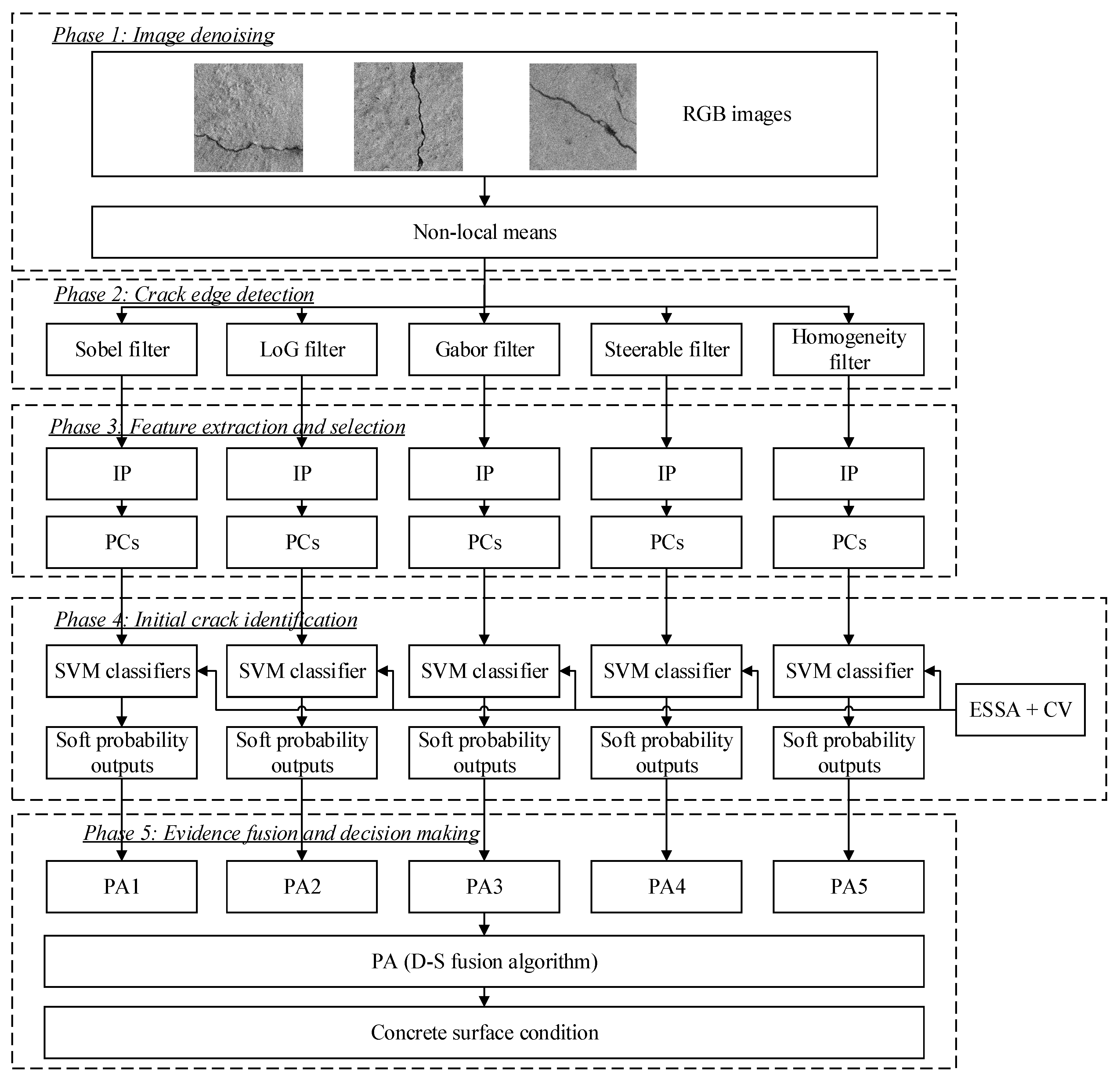
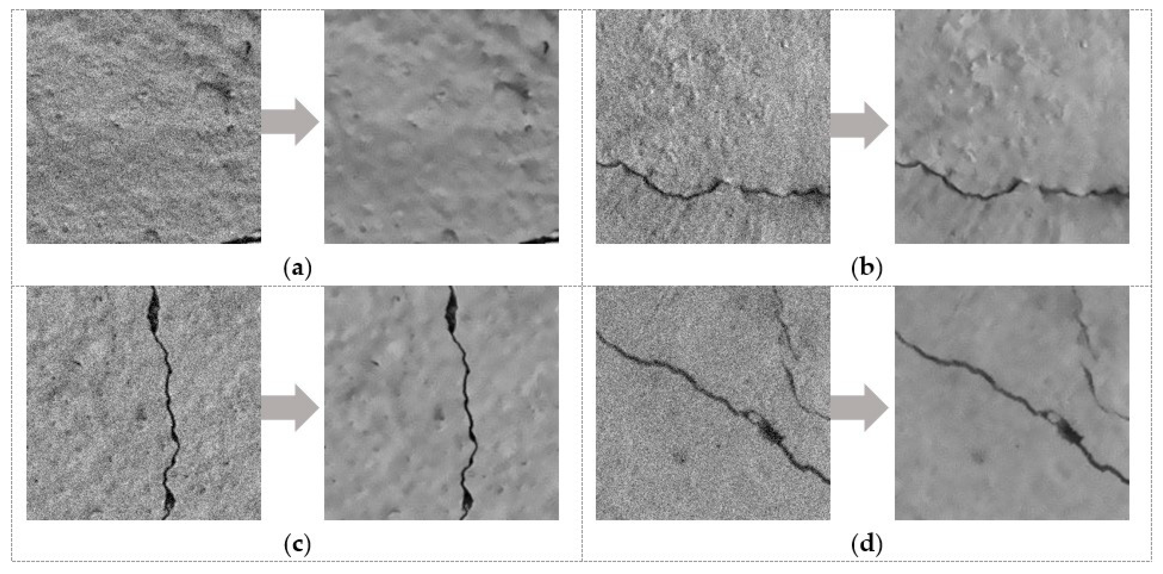
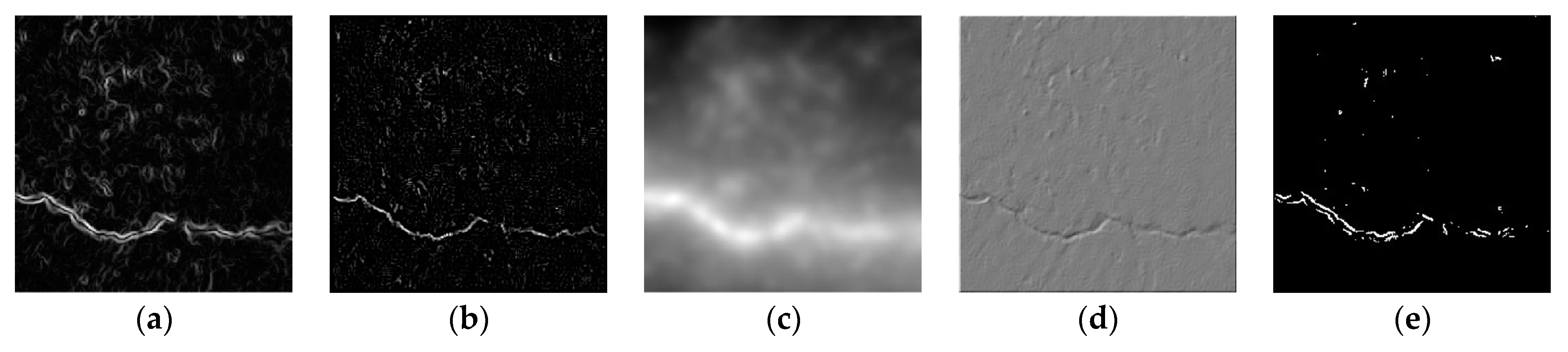
To address the challenges in existing concrete crack identification methods, a hierarchical framework is proposed in this study via combining various image processing, ML and information fusion techniques. To start with, the raw images are denoised using non-local means method. Then, the processed images are sent to different filters for crack edge detection, and the crack sensitive features are extracted by the integral projection. Principal component analysis on the extracted features is also undertaken to select optimal components. The SVM multi-classifiers, with benefits of high-dimensional and nonlinear pattern recognition with small size of samples, are subsequently built up to achieve the initial identification of crack pattern. To improve the generalization capacities of the classifiers, the enhanced salp swarm algorithm is employed to optimize the meta-parameters of SVM. Eventually, the Dempster–Shafter fusion algorithm is introduced to fuse the initial results of different classifiers corresponding to different image filtering methods to improve the identification accuracy. Finally, the concrete images taken by a RPA are used to verify the effectiveness of the proposed framework with satisfactory results.

2. Materials and Methods

2.1. Establishment of Dataset

To establish a dataset for developing concrete crack identification approach, a total of 1287 RGB images, with the resolution of 4608 × 3072 pixels, were captured by a RPA. These images were taken from the surfaces of girder and pier of a concrete bridge under different light conditions containing both shadowed and sun facing surfaces. The image files were saved as JPGs, with the mean size of 6 MB. Since the original images include multiple cracks with various types, each image was cropped into several images with the resolution size of 256 × 256 pixels. All the cropped images can be categorised at four levels, background (without crack), longitudinal crack, transverse crack and oblique crack images. For each category, 300 images are selected and, therefore, a total of 1200 images will be employed in this research. The examples of images with different categories are shown in Figure 1.

2.2. Proposed Hierarchical Framework

The schematic of the proposed hierarchical framework is displayed in Figure 2. As shown in the figure, the framework is divided into four analysis phases, i.e., image pre-processing, crack edge detection, feature extraction and selection, and crack pattern identification. In the phase of pre-processing, the non-local means algorithm is employed to deal with the raw images to eliminate the noise interference. In the second phase, the denoised images are processed by five adaptive filters, including Sobel, Laplacian of Gaussian (LoG), Gabor, steerable and homogeneity filters, for crack edge detection. In the third phase, crack-sensitive features are extracted and normalized using the integral projection method. To prevent feature information redundancy and decrease the feature dimension, principal component analysis is introduced to select optimal components to stand for whole feature information. Based on selected principal components, the SVM classifiers with posterior probability outputs are built up in the fourth phase, which provide the initial identification results. To ameliorate the generalization capacities of SVM classifiers, the enhanced salp swarm optimization (ESSO) algorithm and cross-validation (CV) operation are employed to optimize the SVM meta-parameters during the model training. In the fifth phase, the posterior probability outputs of SVM, regarded as the evidences, are transformed into the basic probability assignments (PAs), and the D–S evidence fusion algorithm is used to fuse the initial results obtained from different filters to give a final result. Since the initial identification results from different filters may be either inaccurate or conflicting, the fusion of these results is capable to effectively avoid the wrong identification. It is noticeable that the proposed framework adopts a hierarchical architecture, where the outputs in the former phase are the inputs in the next phase. Hence, via multi-phase image processing, the identification accuracy and robustness of concrete crack can be guaranteed.

3. Image Denoising and Crack Edge Detection

3.1. Original Image Pre-Processing Using Non-Local Means Method

Identifying the crack pattern on the surface of concrete structure is challenging due to complicated textures of concrete background and inhomogeneous intensity of crack. The general textures of concrete structure consist of aggregate and cement with various shapes and colours, which may be inaccurately recognized as the crack. On the other hand, some cracks could not be identified because of the fact that they have similar intensities as the background object due to several factors such as lighting condition, narrow width of crack (e.g., micro-crack) and noise influence. To improve the crack identification accuracy, it is of great necessity to eliminate the effect of background textures of concrete surface using image denoising method.
The non-local means (NLM) is a denoising technique that aims to deal with Gaussian white noise in natural images [37]. The fundamental of NLM is to construct the weighting of mean value by means of evaluating the similarity of patch pixels of image, which is different from traditional methods using single pixel similarity. Therefore, image denoising using patch information is capable of better keeping the edges, textures and other features of image as seen in Figure 3. Suppose there is a noisy image denoted by v = { v ( a ) | a A } , where A denotes the coordinate domain of image. For any pixel a in the image, the estimated value of this pixel using NLM can be calculated by:
N L M [ v ] ( i ) = b A w f ( a , b ) v ( b )
where the weighting function w f ( a , b ) relies on the similarity degree between pixels a and b, and meets the conditions 0 w f ( a , b ) 1 and b w f ( a , b ) = 1 .
The similarity degree between pixels a and b is determined by the grey matrices Na and Nb, which denote the image regions centre on pixels a and b, respectively. The similarity between two regions Na and Nb can be measured by the Gaussian weighted Euclidean distance d g ( a , b ) , shown as:
d g ( a , b ) = | | v ( N a ) v ( N b ) | | 2 , ϑ 2
where ϑ denotes the standard deviation of Gaussian kernel. The more similar the grey matrices between neighbouring regions, the greater the weighting of corresponding pixels in the weighted average. The weighting function wf(a,b) is defined as follows:
w f ( a , b ) = 1 Z ( a ) e d g ( a , b ) r 2
Z ( a ) = b e d g ( a , b ) r 2
where Z(a) is a normalized parameter; r denotes the smoothing parameters, which is related to the standard deviation of image noise.

3.2. Crack Edge Detection Using Filtering Methods

After the denoising, the pre-processed images are further dealt with for crack edge detection. It is generally acknowledged that the light intensities between non-cracked and cracked images are remarkably different, so the nonlinear filters can be utilized to distinguish the difference in light intensity for crack edge detection. In this study, five different types of filters are used to achieve this objective.

3.2.1. Sobel Filter

The fundamental of the Sobel filter is to conduct the weighted smoothing on the image, and then carry out the differential operation [38]. The related mathematical expressions are given as follows:
G x = [ f ( i + 1 , j + 1 ) + 2 f ( i , j + 1 ) + f ( i 1 , j + 1 ) ] [ f ( i 1 , j 1 ) + 2 f ( i , j 1 ) + f ( i + 1 , j 1 ) ]
G y = [ f ( i 1 , j 1 ) + 2 f ( i 1 , j ) + f ( i 1 , j + 1 ) ] [ f ( i + 1 , j + 1 ) + 2 f ( i + 1 , j ) + f ( i + 1 , j 1 ) ]
The gradient value of pixel point (i,j) can be calculated by:
M ( i , j ) = | G x | + | G y |
The crack edges in the image can be determined according to this gradient value. Given the threshold Ts, if M ( i , j ) T s , the pixel is regarded as the edge point; otherwise, it is a non-edge point. In this study, the value of is set at 3.73, as suggested in [18].

3.2.2. Laplacian of Gaussian (LoG) Filter

A LoG filter was developed based on Laplacian operator, which is the derivative filter utilized for localizing the areas of abrupt changes in the image [39,40]. In this filter, before the Laplacian operation is applied, the Gaussian filter is employed to smoothen the image. Consequently, it is called LoG filter. Laplacian operator can be defined as follows:
2 f ( x , y ) = 2 f ( x , y ) x 2 + 2 f ( x , y ) y 2
In this study, the four neighbours-differential kernel is employed to approximate Laplacian differential operation, which is shown as follows:
M ( i , j ) = | 4 f ( i , j ) f ( i , j 1 ) f ( i 1 , j ) f ( i + 1 , j ) f ( i , j + 1 ) |
where (i,j) denotes the pixel point in the image. To add the Gaussian filter for image smoothing, the function that combines both Gaussian and Laplacian filters can be represented by:
2 G l ( x , y , ρ ) = 1 2 π ρ 2 ( x 2 + y 2 ρ 2 2 ) e x 2 + y 2 2 ρ 2
where ρ denotes the width of Gaussian kernel.

3.2.3. Gabor Filter

A two-dimensional (2D) Gabor filter was first proposed by Daugman, which can be regarded as a complex sine function modulated by Gaussian function [41]. Similar to the 2D receptive field profile of simple cells in mammalian visual cortex, the 2D Gabor filter has excellent spatial locality and directional selectivity, and is able to capture special frequency and local structural features of multiple directions in the local region of the image. The definition of the 2D Gabor filter is shown in Equation (11):
G a ( x 0 , y 0 , θ , ω 0 ) = 1 2 π σ 2 e x 0 2 + y 0 2 2 σ 2 · [ e j ω 0 x 0 e ω 0 2 σ 2 2 ] x 0 = x · cos ( θ ) + y · sin ( θ ) y 0 = x · sin ( θ ) + y · cos ( θ )
where (x,y) denotes the pixel point in the image; ω 0 denotes the centre frequency of the filter; θ indicates the direction of the Gabor wavelet; and σ denotes the standard deviation of the Gaussian function.
In the image processing, the concrete crack image can be convoluted with the Gabor filter, and the corresponding result of convolution is the extracted Gabor features. Assume f(x,y) is the image of concrete crack, the convolutional operation between f(x,y) and G a ( x 0 , y 0 , θ , ω 0 ) can be expressed by the following equation:
F ( x 0 , y 0 , θ , ω 0 ) = f ( x , y ) G a ( x 0 , y 0 , θ , ω 0 )
where “⨂” denotes the convolutional operation.

3.2.4. Steerable Filter

Since the images can be represented by directional features, the detectors of directional features are basic tools in image feature extraction. The steerable filter, developed by Adelson and Freeman, is one type of directional feature detector [42]. Its principle is to realize the response of a filter in any direction by linear combination of a group of basic filters in different directions. The response can be considered as a function of direction angle, which can be controlled to determine the output of the filter. In the steerable filter, second-order partial derivative of the two-dimensional Gaussian function is employed as the tuneable filter due to its good characteristics of directionality, separability and self-similarity. The expression of the two-dimensional Gaussian function at the pixel point (z1, z2) of image can be expressed by Equation (13):
G ( z 1 , z 2 ; ρ ) = e z 1 2 + z 2 2 2 ρ 2 2 π ρ 2
where ρ denotes the inner scale, which determines the width of kernel. 1 / 2 π ρ denotes the normalization factor. The second-order partial derivatives of G ( z 1 , z 2 ; ρ ) can be expressed by:
G z 1 z 1 ( z 1 , z 2 ; ρ ) = z 1 2 ρ 2 2 π ρ 6 e z 1 2 + z 2 2 2 ρ 2      
G z 2 z 2 ( z 1 , z 2 ; ρ ) = z 2 2 ρ 2 2 π ρ 6 e z 1 2 + z 2 2 2 ρ 2
G z 1 z 2 ( z 1 , z 2 ; ρ ) = G z 2 z 1 ( z 1 , z 2 ; ρ ) = z 1 z 2 2 π ρ 6 e z 1 2 + z 2 2 2 ρ 2
Consequently, the steerable filter can be formulated by Equation (17):
S F ( z 1 , z 2 ; ρ , α ) = sin 2 ( α ) G z 2 z 2 ( z 1 , z 2 ; ρ ) + 2 sin ( α ) cos ( α ) G z 1 z 2 ( z 1 , z 2 ; ρ ) + cos 2 ( α ) G z 1 z 1 ( z 1 , z 2 ; ρ )
where α denotes the directional angle of filter. Based on Equation (17), the responses of pixel point (z1, z2) in image Q can be calculated by the following equation:
R p ( z 1 , z 2 ) = S F ( z 1 , z 2 ; ρ , α ) Q ( z 1 , z 2 )
where “ ” denotes the convolutional operation as before.

3.2.5. Homogeneity Filter

The homogeneity filter was developed based on the homogeneity operator, in which the pixel is subtracted by its eight neighbouring pixels [43]. The mathematical expression of the homogeneity operator is shown in Equation (19):
H P = { max ( { | I P I N i | } ) , i f   I P   > I t 0 , o t h e r w i s e
where P denotes the central pixel; Ni denotes the ith neighbour of the central pixel, i = 1,2,…,8; IP denotes the intensity of the central pixel; It denotes the pre-set threshold, ranging between 0 and 255. In this work, the value of It is calculated by Ostu method.
Figure 4, Figure 5 and Figure 6 demonstrate the examples of comparison of different filters in processing the crack images, respectively. It is clearly observed from these figures that most filters are effective in detecting the edges of different types of crack, even though some small regions in the images are inaccurately identified as the cracks. Overall, the processed grey images by the filters can be used to extract the features as the inputs of the machine learning classifiers.

4. Crack-Sensitive Feature Extraction and Selection

Based on the filtered images, the crack-sensitive features are extracted and selected based on integral projection and principal component analysis. The detailed process and results will be presented in the following sub-sections.

4.1. Feature Extraction Using Integral Projection

The integral projection (IP) was developed on basis of the projection distribution characteristics of the image in some directions [44]. As a statistical approach, the IP essentially consists of horizontal projection and vertical projection, the expressions of which are given as follows:
H ( y ) = x = 0 n 1 I ( x , y )
V ( x ) = y = 0 m 1 I ( x , y )
where (x,y) denotes the pixel location and I(x,y) denotes corresponding pixel intensity. n denotes the number of all pixels in row and m denotes the number of all pixels in column.
In this study, the IP is employed to characterize different patterns of concrete crack. After the concrete surface images are processed by the nonlinear filters, the values of IP can be calculated and each type of crack will possess unique IP property. Generally, the longitudinal crack always leads to the stable IP in the X-axis (horizontal axis) but a peak intensity of IP in the Y-axis (vertical). On the contrary, the transverse crack causes a peak intensity of IP in the X-axis but stable IP in the Y-axis. Unlike longitudinal and transverse cracks, both without crack and oblique crack have constant IPs in both horizontal and vertical axes. Moreover, the filtering result of image with oblique crack can reflect the intensity value of crack texture, and the mean value of IP of oblique crack is higher than that of without crack. Figure 7 demonstrates the results of IP for the cases with different types of cracks processed by the LoG filter. As discussed above, the image of longitudinal crack has the peak pixel intensity of 31.43 in the vertical axis while image of transverse crack possesses the maximum pixel value of 62.51 in the horizontal axis. The mean value of pixel intensities of IP of image with oblique crack is around 9.30, which is obviously higher than that of the without-crack case (7.20). Accordingly, the IPs can be used as good indicators to distinguish different scenarios of concrete surface.

4.2. Optimal Feature Selection Using Principal Component Analysis

If all the IPs are used as the inputs to develop the diagnostic models, the model configuration will be much more complicated due to high dimension of the features. In addition, the IPs may contain the redundant information that can affect the generalization capacity of trained model. As a result, it is better to employ fewer significant components to stand for all the IPs as the optimal features. In this research, the problem is addressed by using principal component analysis (PCA), which aims to reduce the dimension of observed variables and obtain the most important information via transforming multiple variables into a few components [45]. The principle of PCA is summarized as follows. Suppose the matrix of n observations of original variable X is X = ( X 1 , X 2 , , X p ) = [ x 11 x 1 p x n 1 x n p ] , and the algorithm process of PCA can be summarized in the following steps:
(1) Normalize the original data using Equations (22)–(24):
X ¯ j = 1 n d i = 1 n d x i j    
σ j = i = 1 n d ( x i j X ¯ j ) 2 n 1
x i j = x i j X ¯ j σ j
where i = 1, 2, …, n; X ¯ j and σ j denote the mean value and standard deviation of samples, respectively, and j = 1, 2, …, p.
(2) Calculate the correlation coefficient matrix M using Equation (25):
M = 1 n d ( X ) T X = [ m 11 m 1 p m p 1 m p p ]
where m i j = m j i and m i i = 1 .
(3) Calculate the eigenvalue and eigenvector of M. According to the eigen equation | M λ E | = 0 , the eigenvalue λ j and eigenvector U j = ( U 1 j ,   U 2 j ,   ,   U p j ) ,   ( j = 1 ,   2 ,   ,   p ) can be obtained, where λ 1 λ 2 λ p 0 . The extracted principal components (PCs) can be represented by Y j = X j U j , that is:
y j = x k 1 U 1 j + x k 2 U 2 j + + x k p U p j   ( k = 1 ,   2 ,   ,   n ; p = 1 ,   2 ,   ,   n )
(4) Determine the number of PCs. The individual and accumulated contributions of PCs can be expressed by:
η i = λ i i = 1 p λ i
η Σ ( m ) = i = 1 m η i
By PCA, the IPs can be replaced with 512 PCs in the decreasing order of individual contributions. Figure 8 demonstrates an example of PCA results of images processed by the Sobel filter, in which both individual and accumulative contributions of PCs are displayed. It is observed that the first two PCs have the highest contribution rates of 26.87% and 26.41%, respectively. From the third PC, the contribution percentages of PCs reduce to below 10%, while the accumulative contribution percentage can continuously ascend. The first 15 PCs can achieve more than 95% contributions of all the IPs. Even though around 5% feature information of IPs is lost, the feature dimension is significantly reduced, which is beneficial to the model training of the classifier. Based on the same selection criteria (>95% contributions), the numbers of selected PCs for the LoG filter, Gabor filter, steerable filter and homogeneity filter are 22, 17, 15, 25 and 32, respectively.

5. Feature Level-Based Crack Diagnosis Using Enhanced Salp Swarm Algorithm-Optimized SVM Classifiers

In this section, corresponding to each filtering method, the classifier based on SVM will be developed to automate the concrete crack identification. To improve the generalization capacity of SVM, an enhanced salp swarm algorithm is proposed to optimize the meta-parameters during the model training.

5.1. SVM Sub-Classifiers for Identifying Concrete Crack

The typical application of SVM is for solving binary classification problem, i.e., judging whether the test sample belongs to positive or negative class [46]. However, this study aims to identify different crack types of concrete, which is a multi-objective classification problem in nature. One of the most direct ways is to construct multiple hyperplanes, which can be used to divide the entire sample space into multiple regions. Each region corresponds to one class. Although this method is able to fundamentally solve this problem, its application prospect is not encouraging due to a large amount of calculation. In the practical application, there are two common strategies to solve such a multi-classification problem: one against rest (OAR) and one against one (OAO). The fundamental of these two strategies is to transform a multi-classification problem into multiple binary-classification problems. The corresponding classifier is also called “sub-classifier”. For an n-class classification problem, the OAR strategy only requires to establish C n 1 = n sub-classifiers. In i-th sub-classifier, the samples with i-th class are regarded as the positive class samples, while the rest of the samples are regarded as the negative class samples. The final classification result of OAR strategy is the output category of positive class. The main benefit of OAR strategy is that the number of sub-classifiers needed to be established is relatively small, but there exists the potentials of “classification overlap” and “unclassifiable”. The OAO strategy, however, establishes the sub-classifiers for any arbitrary two classes of samples in the n-class classification problem, and a total of C n 2 = n ( n 1 ) / 2 sub-classifiers are required. The final classification result of OAO strategy is decided by the voting of all the sub-classifiers. The main feature of OAO strategy is that the number of sub-classifiers is rapidly increased with the adding class number and the training efficiency is lower than that of OAR strategy.
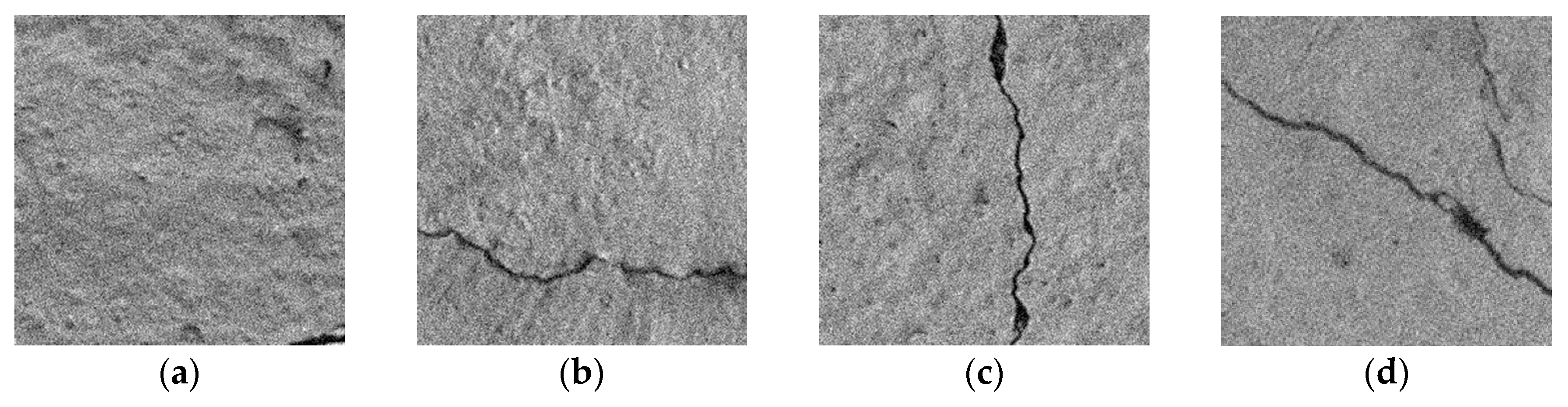
In this work, both OAR and OAO strategies are investigated to develop SVM sub-classifiers for concrete surface crack identification. Hence, four ( C 4 1 = 4 ) sub-classifiers should be developed for the OAR strategy, i.e., without crackrest (MWAR), longitudinal crackrest (MLAR), transverse crackrest (MTAR) and oblique crackrest (MOAR) sub-classifiers, while six ( C 4 2 = 6 ) sub-classifiers need to be trained for the OAO strategy, i.e., without crack–longitudinal crack (MWAL), without crack–transverse crack (MWAT), without crack–oblique crack (MWAO), longitudinal crack–transverse crack (MLAT), longitudinal crack–oblique crack (MLAO) and transverse crack–oblique crack (MTAO) sub-classifiers. For the training and validation of the classifiers, 80% of images of each concrete condition scenario (960) are randomly selected as training data to develop the sub-classifiers, while the rest of the images (240) are employed as validation samples to evaluate the performance of trained sub-classifiers.

5.2. Optimizing Meta-Parameters of SVM Using ESSA

The fundamental of SVM is to find an optimal classification line which can not only separate the data samples correctly but also maximize the margin. For the data with nonlinear separability, the samples in the input space can be mapped to the high-dimensional feature space through the nonlinear transformation, which transforms the nonlinear classification into linear transformation and forms a nonlinear SVM. However, SVM is not capable of directly solving the dot product of the feature space, so the kernel function of original space is employed instead. There are a number of functions that can be used as the kernel of SVM, including polynomial function, radial basis function (RBF), sigmoid function, etc. In this study, the RBF is selected due to wider domain of convergence. The mathematical expression of RBF is:
K ( x i · x ) = exp ( | | x i x | | 2 2 σ 2 )
where σ is a free parameter to indicate the variance of kernel. The optimal classification function can be written as:
f ( x ) = s g n ( i = 1 m y i α i K ( x i · x ) + b )
where α i ( i = 1 , 2 , , m ) are optimal Lagrange multipliers in the range of (0, C) and b denotes the bias.
When the SVM-based sub-classifiers are established for concrete crack identification, the meta-parameters of SVM should be appropriately selected. Here, the SVM meta-parameters include balance coefficient C and kernel parameter σ. The influences of both parameters on the SVM performance are totally different. For parameter C, if it is assigned with a low value, the classification function will be flat; if it is assigned with a high value, more samples will be employed as the support vectors to accurately predict all the data. Different settings of parameter combination may result in distinctly different model performances [47]. Accordingly, how to select the optimal values of meta-parameters is of great importance to the development of SVM for the best generalization ability. In this study, an enhanced salp swarm algorithm (ESSA) is put forward to optimize the C and σ during the training of SVM sub-classifiers. The fitness function of meta-parameter optimization is defined as the mean prediction accuracy of training samples using five-fold cross validation (CV), and the optimization problem can be expressed by:
max R A 5 C V ( C , σ 2 ) = N o .   o f   c o r r e c t   p r e d i c t i o n s N o .   o f   a l l   t h e   p r e d i c t i o n s × 100 %   s . t .   σ m i n 2 σ 2 σ m a x 2 ,   C m i n C C m a x
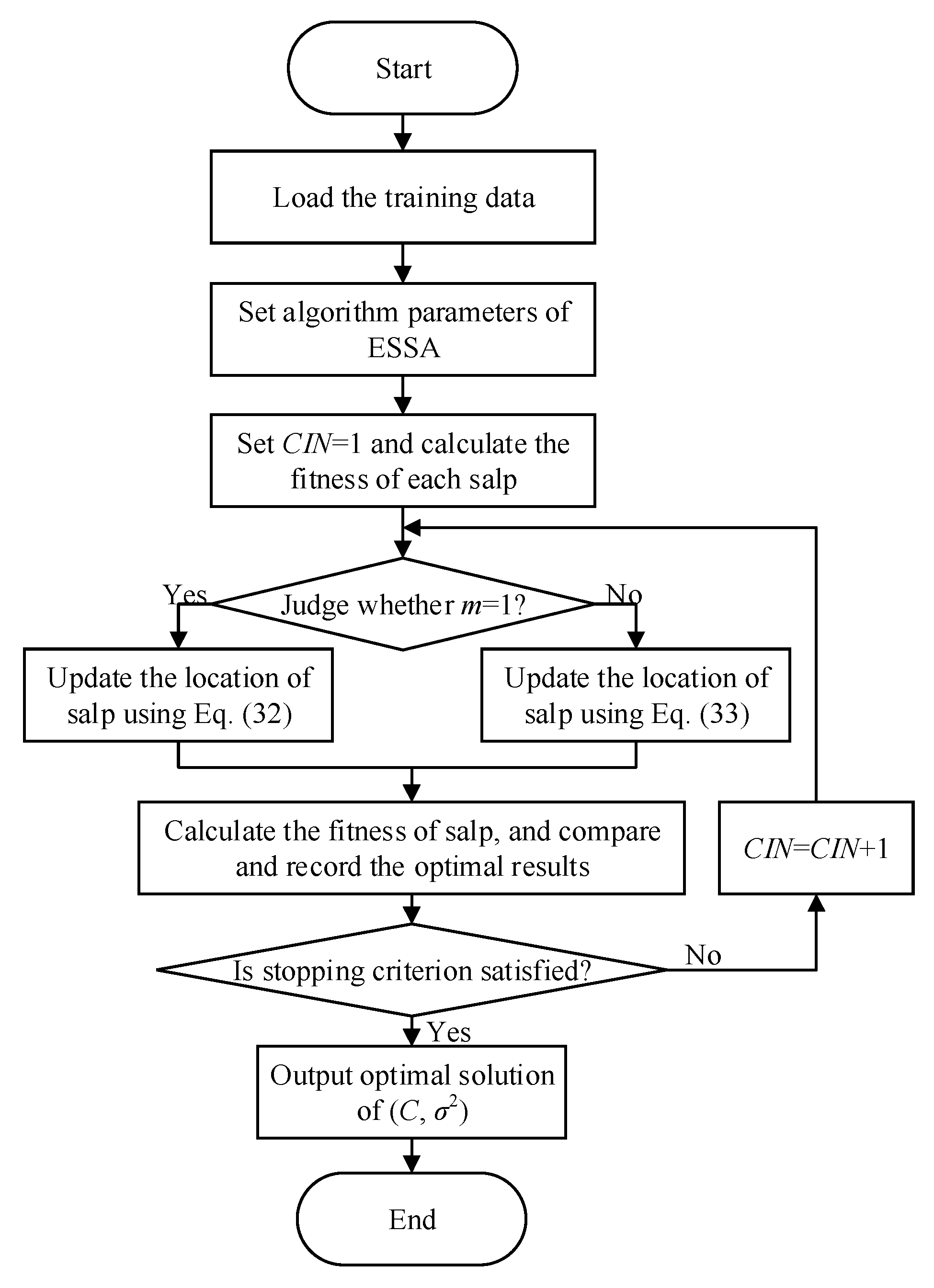
The procedure of using ESSA to optimize the meta-parameters of SVM sub-classifiers can be summarized as follows, which is also shown in Figure 9.
Step 1. Confirm the optimization target and the parameters to be optimized, and set the algorithm parameters of ESSA, including swarm size of salp, maximum iteration number and parameters affecting S-curve-based decreasing weight.
Step 2. Initialize the locations of the salps in the vector of parameters to be optimized. Here, the parameters are C and σ2, and the upper and lower boundaries of parameters are 0.001 and 100, respectively.
Step 3. Calculate the fitness value of each salp in the swarm, and record the individual optimum and global optimum of the swarm.
Step 4. Set current iteration number CIN as 1.
Step 5. For each salp, if it is the leader (first salp, m = 1), use Equation (32) to update its location; otherwise, use Equation (33) to update the location:
X d 1 = { w F d + c 1 [ ( u b d l b d ) c 2 + l b d ] ,   c 3 0.5 w F d c 1 [ ( u b d l b d ) c 2 + l b d ] ,   c 3 < 0.5   c 1 = 2 e 4 l l m a x  
X d m = 1 2 ( X d m + X d m 1 ) ,   m 2
where X d 1 denotes the location of the leader; F d denotes the food location; w denotes the weighting factor; u b d and l b d are upper and lower search boundaries; c 2 and c 3 are two random numbers between 0 and 1; c 1 denotes convergence factor, which is used to balance the exploitation and exploration abilities of algorithm; l denotes the current iteration number; lmax denotes the maximum iteration number; X d m denotes the location of m-th follower.
Step 6. Evaluate the fitness value of each salp, and compare the current individual and global optimum with previous ones. If the current results are better, replace the previous record with current results; or else, keep the record unchanged.
Step 7. Judge whether the current iteration number reaches its maximum value. If so, terminate the optimization. Otherwise, CIN = CIN + 1 and go back to Step 5.

5.3. SVM Training Results

In this study, 80% of images of each class are randomly selected as the training samples to develop the SVM sub-classifier while the rest of images are used as the validation samples to evaluate the effectiveness of the proposed model. The setting of basic parameters of ESSA is given as follows: swarm size is 50 and the maximum iteration number is 200. Additionally, how to define the decreasing weight w is also important, since it directly affects the accuracy and convergence of algorithm [48]. Generally, in the initial stage of algorithm evolution, we need a large weighting to enhance the global search ability of ESSA, while in the later stage, a small weighting is required to improve the local search ability. In [
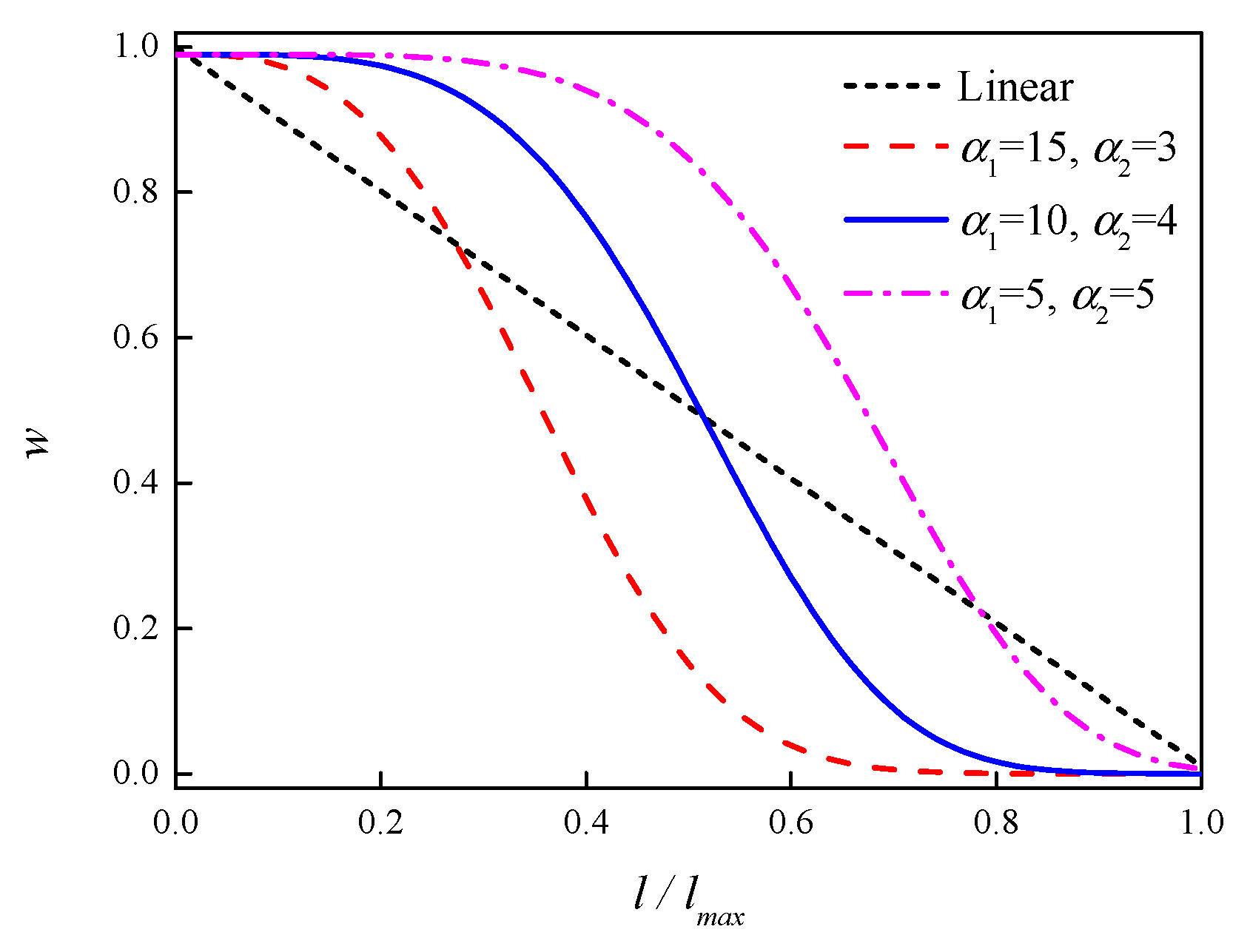
49], a linearly decreasing weighting factor was proposed to update the location of leader salp. However, when it is far from the food source, the SSA with linear decreasing weight may fall into the local optimum. Accordingly, this study corrects this problem and proposes an S-curve-based decreasing weighting factor, with the expression in Equation (34):
w = ( w m a x w m i n ) · e α 1 ( l l m a x ) α 2
where α 1 and α 2 are two parameters to tune the shape of the S-curve. A comparison between S-curve-based decreasing weight with different combinations of α 1 and α 2 and linear decreasing weight is shown in Figure 10. It is clearly seen that compared to the linear one, the nonlinear weighting based on S-curve keeps the larger value for a longer time in the early stage, which can make the leader salp quickly find the rough location of food, and then rapidly declines to the minimum value in the later stage, which is beneficial to the fine tuning of food location. Among three parameter combinations, the combination ( α 1 = 10, α 2 = 4) shows the symmetric property in the range of [0, 1], which is adopted in this study.
Then, the training samples are sent to the SVM for obtaining optimal model parameters based on ESSA. 
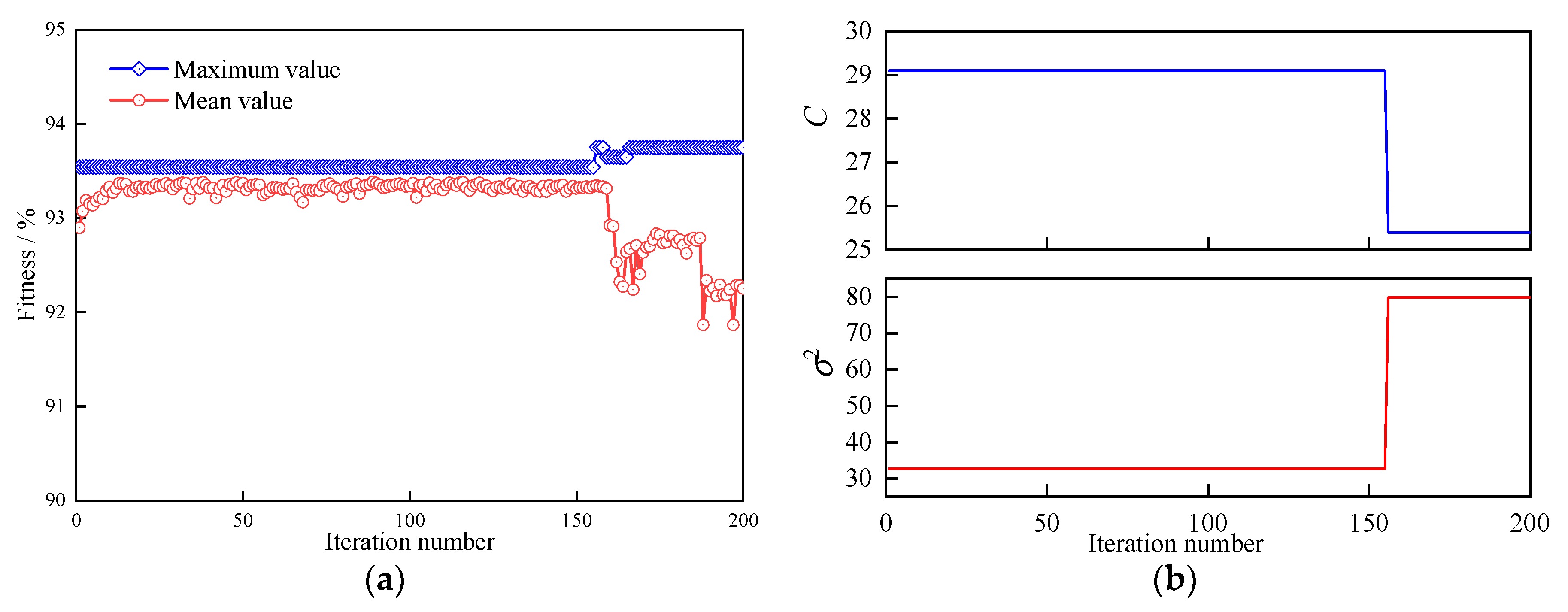
Figure 11 demonstrates an example of SVM meta-parameter optimization of without crack-rest sub-classifier based on the images processed by the Sobel filter, in which Figure 11a depicts optimal and mean fitness with the iteration and Figure 11b shows the optimization process of parameters C and σ2. It can be observed that the maximum identification accuracy is kept at a relatively stable value of about 93.8%, while the mean identification accuracy fluctuates between 92% and 94%. For two SVM parameters, their values have obvious variations at around 155th iteration, and then arrive at the optimal values of 25.3911 and 79.8106, respectively. Table 1 summarizes the details of all trained SVM sub-classifiers including optimal meta-parameters and number of support vectors. Based on the best meta-parameters, the trained sub-classifiers can obtain the optimal generalization capacity for concrete crack identification.

6. Decision Level-Based Crack Diagnostic Enhancement Using Dempster–Shafer (D–S) Fusion

6.1. Dempster–Shafer Fusion Algorithm

In this research, the D–S fusion algorithm is employed to combine the initial diagnostic results of concrete surface corresponding to different filters. In the D–S fusion, the frame of recognition χ should be established first to include all the potential categories of concrete surface condition. Here, χ is defined as χ = [η1, η2, η3, η4], where η1, η2, η3 and η4 correspond to intact, longitudinal crack, transverse crack and oblique crack, respectively. In addition, the basic probabilities are assigned to all the possible hypothesis in the frame of recognition, satisfying the condition in Equation (35):
V 2 χ m ( V ) = 1 m ( Ø ) = 0
where m(·) is called probability assignment (PA) function, which can assign the subset in 2χ with a value between 0 and 1. Hence, m(V) corresponds to each evidence.
In this work, the D–S algorithm is adopted to fuse the initial diagnostic results of an image from different SVM sub-classifiers and image filtering methods. Suppose the numbers of sub-classifiers and image filtering methods are m and n, respectively, there are a total of m·n identification results for one test image, corresponding to m·n pieces of evidence, denoted by m1, m2, …, mm·n. The fusion of these pieces of evidence can be considered as the operation of conjunctive summation, expressed by [50,51]:
m ( V ) = 0 , V = Ø m ( V ) = m 1 m 2 m m · n = 1 1 C P V 1 V m · n = V m 1 ( V 1 ) m m · n ( V m · n ) , V Ø   C P = V 1 V m · n = Ø m 1 ( V 1 ) m m · n ( V m · n )
where CP denotes the conflict degree among different pieces of evidence. Final diagnostic result of concrete surface can be made according to maximum degree of subset in 2χ. For any element Vi, if the following condition is met,
m ( V k ) = max ( m ( V j ) ) ,   V j 2 χ ,   V k V i m ( V i ) m ( V k ) > τ 1 m ( V i ) > m ( Θ ) m ( Θ ) < τ 2
Vi is the fusion result. In Equation (37), τ 1 and τ 2 are the pre-set thresholds that can guarantee the identification accuracy. Θ represents all the possible condition combinations, and its probability assignment corresponds to the uncertainty of the final result. To reduce the influence of uncertainty on the result accuracy, τ 1 and τ 2 are set to 0.3 and 0.1 in this study, according to the suggestion in [52].

6.2. Soft Outputs of SVM Sub-Classifier

The class information of sample outputted from standard SVM can always be given clearly, that is, 0 (negative) and 1 (positive), which belongs to “hard” decision. However, in the real situation, for some uncertain classification problems, it is difficult to categorize the samples into a certain class, but instead can give the probability value or membership degree to any class. If the SVM is used to deal with the non-deterministic classification, the “soft” decision is needed. Generally, the identification result of standard SVM can be mapped into the interval of [0, 1] to realize the probability output, which is used to signify the uncertainty of the result. In this research, the sigmoid function is selected as the posterior probability model, the expression of which is shown in Equation (38):
p o ( x ) = 1 1 + e [ M f ( x ) + N ]  
This function can be with different forms via tuning the parameters of M and N. To satisfy the condition that the output of po(x) monotonically increases with the probability value of positive class, the value of M should be negative. Adjusting parameter N can make the SVM with the ability to deal with the bias training data. Selecting optimal values of M and N can be regarded as solving the following optimization problem:
m i n i m i z e k = 1 m [ t o k ln ( p o k ) + ( 1 t o k ) ln ( 1 p o k ) ] p o k = 1 1 + e [ M f ( x k ) + N ]   a n d   t o k = 1 + y k 2  
The SVM with soft decision can adopt the D–S fusion algorithm to make joint decision. To begin with, the posterior probability output of SVM should be transformed to the probability assignment of D–S fusion. The probability assignments of positive and negative classes are easily determined, i.e., po(x) and 1‒po(x), respectively. However, according to the fundamental of D–S fusion algorithm, the probability assignment of uncertainty in the frame of recognition Θ should be included as well. Here, the uncertainty is defined as the upper boundary of expectation of misclassification rate of test samples, which can be calculated by the following equation:
U E ( E r ) E ( N s u p ) N t r 1  
where the numerator is the average number of support vectors, and Ntr denotes the total number of training data. To meet the requirement that the summation of probability assignments is equal to 1, the outputs of positive and negative classes should be multiplied by the coefficient 1 max [ U E ( E r ) ] . Accordingly, the mathematical expressions of probability assignments of SVM sub-classifier are given as follows:
{ m ( P C ) = p o ( x ) ( 1 N s u p N t r 1 ) m ( N C ) = [ 1 p o ( x ) ] ( 1 N s u p N t r 1 ) m ( Θ ) = N s u p N t r 1
where PC and NC denote positive and negative classes, respectively.

6.3. Fusion Results and Discussion

To evaluate the performance of proposed method, the test images with different concrete surface conditions are processed and then inputted into the trained SVM sub-classifiers for initial diagnosis. As an example, Table 2, Table 3, Table 4 and Table 5 list the probability assignments of four SVM sub-classifiers in the OAR strategy for an image without a crack. Table 2 displays the assignment values of without crack-rest sub-classifier, in which m1,i (i = 1, 2, …, 5) correspond to the initial diagnostic results with different image filtering methods. As can be seen from the table, more confidences are assigned to without crack proposition (V1) than to rest proposition (V2 V3 V4) conforming to the real condition, except the case of Gabor filter (m1,3) where the assignments of without crack and rest are 0.1766 and 0.2802, respectively. Nevertheless, it is hard for the system to make a diagnostic decision, since the uncertainty ( Θ ) has the largest probability assignment in each evidence, obviously exceeding the pre-set threshold value of 0.1. The major reason causing this problem is that the number of support vectors is relatively higher compared to the total number of training samples. The probability assignments of the other three sub-classifiers (longitudinal crack-rest, transverse crack-rest and oblique crack-rest) for this image without a crack are provided in Table 3, Table 4 and Table 5. Like the without crack-rest sub-classifier, these three sub-classifiers allocate more probability assignments to rest proposition (V1 V3 V4, V1 V2 V4 or V1 V2 V3) than longitudinal crack-rest (V2), transverse crack-rest (V3) or oblique crack-rest (V4) proposition. Similarly, the uncertainty with the largest assignment results in the difficulty of decision making of concrete surface condition diagnosis corresponding to each filtering method.
Therefore, the D–S algorithm is applied to the probability assignments of initial diagnostic results via a two-level fusion. In the first-level fusion, at each sub-classifier the assignment results of different image filtering methods are combined, the result of which is shown in Table 6. It is noted that the probability assignment of without crack (V1) is increased to 0.8343 while the uncertainty is decreased to 0.0641 for the without crack-rest sub-classifier. Likewise, for the sub-classifiers of longitudinal crack-rest, transverse crack-rest and oblique crack-rest, the assignment values of rest proposition V1 V3 V4, V1 V2 V4 and V1 V2 V3 are ascended to 0.9931, 0.9682 and 0.8939, respectively. The assignments of uncertainties of these three sub-classifiers are all below 0.07. In accordance with the first-level fusion result, we can find that the proposition of without crack is apt to be the diagnosis result of concrete surface. Then, in the second-level fusion, the evidence assignments from different sub-classifiers are fused for final decision making. Table 7 provides the result of second-level fusion, in which the probability assignment of correct proposition without crack (V1) has been increased to 0.9732, which approaches 1. More importantly, the value of uncertainty declines to zero. According to decision rule in Equation (37), the fusion diagnostic result is V1, which is consistent with the real situation of concrete surface (without crack). This example effectively demonstrates that the probability assignments of correct propositions can be significantly increased after two-level data fusion, compared to the diagnostic results without data fusion.
In the same manner, the two-level fusion results of examples of images with longitudinal crack, transverse crack and oblique crack are shown in Table 8, Table 9 and Table 10. Based on the decision rule, the fusion outcomes of three image examples are V2 (longitudinal crack), V3 (transverse crack) and V4 (oblique crack), respectively, bringing into correspondence with the real situations of the images.
Then, the same four image examples are sent to the OAO-based SVM sub-classifiers for the performance evaluation. Table 11, Table 12, Table 13, Table 14, Table 15 and Table 16 give the probability assignments of six OAO-based sub-classifiers for the image of transverse damage. Apparently, for the sub-classifiers of without crack–transverse crack, longitudinal crack–transverse crack, and transverse crack–oblique crack, more probability values are allocated to the right proposition V3 (transverse crack) than V1 (without crack), V2 (longitudinal crack) and V4 (oblique crack), satisfying the real condition of image. However, similar to OAR-based sub-classifiers, the OAO-based SVM sub-classifiers have the same problem of hard decision making, because of high uncertainties in the probability assignment results. Hence, two-level evidence fusion is employed to combine the diagnostic results from different sub-classifiers as well as different image filtering methods. The fusion results are shown in Table 17 and Table 18, where Table 17 corresponds to the result of first-level fusion and Table 18 corresponds to the result of second-level fusion. It is clearly seen that the probability value of proposition V3 is increased to 0.9981 while the uncertainty is eliminated after the evidence fusion operation. In accordance with Equation (37), the diagnostic condition from the proposed framework should be transverse crack, matching the practical condition of this image.
The fusion results of same images of without crack, longitudinal crack and oblique crack by OAO models are provided in Table 19, Table 20 and Table 21, where the probability assignments of correct primitives are 0.7706, 1 and 0.7154, respectively. The corresponding uncertainties are reduced to 0.0004, 0 and 0.0006, respectively. Based on the fusion results of all the image examples, it can be concluded that the data fusion is capable of enhancing the confidence level of correct primitives and weakening the effect of uncertainty on the diagnostic results. Via the result comparison between OAR and OAO sub-classifiers, we can see that OAR strategy can provide more confidence (probability value) to the correct propositions than OAO strategy after two-level data fusion. In contrast, for the D–S fusion algorithm, the OAO SVM sub-classifier needs less computation cost than the OAR sub-classifier. However, with the increase of number of classification class, the number of OAO-based SVM sub-classifiers ( C n 2 , n is the category number) is remarkably increased in comparison with that of OAR-based models ( C n 1 , n is the category number). Accordingly, how to design SVM multi-classifiers should be decided by the real engineering application.
Table 22 summarizes the accuracy performance of different diagnostic models based on all the test images. These evaluated models include the proposed SVM models with data fusion as well as the SVM models with single type of features, such as SVM with Sobel filter-based features (Sobel-SVM), SVM with LoG filter-based features (LoG-SVM), SVM with Gabor filter-based features (Gabor-SVM), SVM with steerable filter-based features (Steerable-SVM) and SVM with homogeneity filter-based features (Homogeneity-SVM). For the SVM with single-type of features, the model accuracies under both OAR and OAO strategies are calculated, and only the better ones are included in Table 22. It can be seen that the proposed SVM models with data fusion have higher accuracy than the independent SVM models with single-type of features in the concrete crack diagnosis. As a result, it can reach a conclusion that with the data fusion, supplementary accurate identification is capable of being realized with various approaches for feature extraction.
Finally, to investigate the contributions of different nonlinear filtering methods to the diagnosis of concrete crack pattern, an ablation study is conducted in terms of diagnostic accuracy of both training and testing imagery data. In this investigation, each filtering method is removed from the proposed framework in turn, and the diagnostic model with the rest filtering methods is then trained for performance evaluation. The results of ablation study are displayed in Table 23. It is obvious to see that Sobel, LoG and steerable filters have predominant effects on the diagnostic accuracy of the proposed framework for both training and testing images, compared to Gabor and homogeneity filters. Overall, OAR strategy-based models have higher accuracy than OAO-based models. Accordingly, in the practical application, under the circumstance of certain accuracy, some filters with fewer contributions may be neglected, which is capable to effectively decrease the online diagnosis time.

7. Conclusions

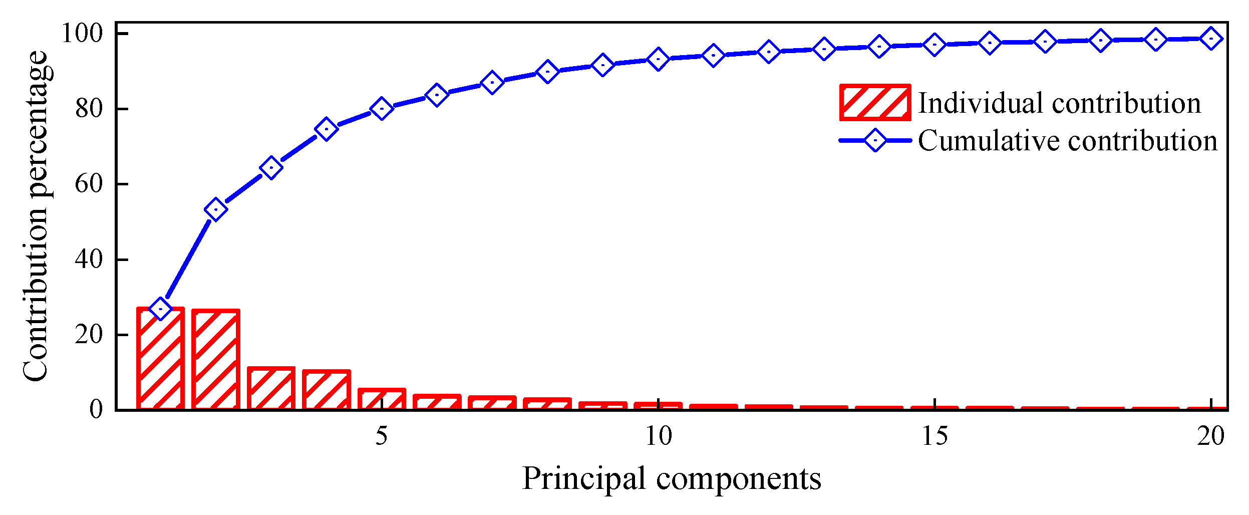
This research develops an intelligent framework for crack diagnosis and classification, which is a combination of signal processing, machine learning, and data fusion techniques. Non-local mean and various filters are employed for noise negation and crack-sensitive pattern recognition, which contribute to a marked diagram of concrete crack. Integral projection, together with PCA, is utilized to diagnose different types of condition surface condition, including without crack, transverse crack, longitudinal crack and oblique crack. The analysis result reveals that the first 15 PCs possess more than 95% feature of all the IPs calculated from the results of the Sobel filter. The reduction of number of features to be learned can enhance the performance of machine learning model. Then, the SVM classifiers with soft outputs under both OAR and OAO strategies are established to conduct initial diagnosis of concrete surface condition. To enhance the generalization ability of the trained classifiers, the ESSA is selected to optimize the meta-parameters of SVM. The optimization results show that the classification accuracy of trained model that can arrive at is as high as 93.8% for the training samples. To fix the problem of wrong or conflicting diagnosis due to different filters, the D–S fusion algorithm is adopted to combine the initial diagnostic results of different sub-classifiers as well as different filters, which are regarded as independent evidences. The fusion results show that the confidence probability of correct proposition can reach 0.99 while the uncertainty of the prediction is reduced to below 0.001 after two-level fusion. In addition, a comparative study demonstrates that the proposed framework outperforms the independent SVM models with single-type of features in terms of the concrete crack diagnosis. Consequently, on the basis of promising results in this research, the proposed framework can be considered as a potential tool for the automatic and real-time structural inspection by the structural engineers and infrastructure agencies.
In this research, the main target is to develop the diagnostic model based on machine learning and data fusion for classifying different patterns of concrete crack. However, in the real situation, the concrete crack pattern may be more complex than three patterns in this study. Accordingly, crack segmentation is necessary for extracting important features of complex cracks including crack width, length and orientation. In the future work, more concrete images with various complex patterns of crack, including V-shape and cross-shape crack, will be collected in the field, and deep learning methods will be employed as the potential tools to fix this problem via building the diagnostic model based on the pre-processed images and corresponding ground truths. In addition, the normalisation operation will be conducted on the raw images to evaluate its effectiveness on the improvement of diagnosis accuracy.

Author Contributions

Conceptualization: Y.Y., M.R. and B.S.; methodology: Y.Y.; validation: Y.Y., A.M.Y. and W.W.; formal analysis: Y.Y., A.M.Y. and W.W.; data curation: Y.Y.; writing—original draft preparation: Y.Y., A.M.Y. and W.W.; writing—review and editing: M.R. and B.S.; supervision: M.R. and B.S.; project administration: M.R. and B.S.; funding acquisition: M.R. and B.S. All authors have read and agreed to the published version of the manuscript.

Funding

This research received no external funding.

Institutional Review Board Statement

Not applicable.

Informed Consent Statement

Not applicable.

Data Availability Statement

The data are not publicly available due to the confidentiality of the research project.

Acknowledgments

The authors acknowledge technical and financial supports from the industry partner Transport for NSW.

Conflicts of Interest

The authors declare no conflict of interest.

References

  1. Avci, O.; Abdeljaber, O.; Kiranyaz, S.; Hussein, M.; Gabbouj, M.; Inman, D.J. A review of vibration-based damage detection in civil structures: From traditional methods to Machine Learning and Deep Learning applications. Mech. Syst. Signal Process. 2021, 147, 107077. [Google Scholar] [CrossRef]
  2. Rashidi, M.; Mohammadi, M.; Kivi, S.S.; Abdolvand, M.M.; Truong-Hong, L.; Samali, B. A Decade of Modern Bridge Monitoring Using Terrestrial Laser Scanning: Review and Future Directions. Remote. Sens. 2020, 12, 3796. [Google Scholar] [CrossRef]
  3. Das, S.; Saha, P. Performance of Swarm Intelligence based Chaotic Meta-Heuristic algorithms in Civil Structural Health Monitoring. Measurement 2020, 169, 108533. [Google Scholar] [CrossRef]
  4. Rashidi, M.; Zhang, C.; Ghodrat, M.; Kempton, S.; Samali, B.; Chiniforush, A.A.; Zhu, L. Bridge Abutment Movement and Approach Settlement—A Case Study and Scenario Analysis. Int. J. Struct. Stab. Dyn. 2018, 18, 1840011. [Google Scholar] [CrossRef]
  5. Abdellatif, M.; Peel, H.; Cohn, A.G.; Fuentes, R. Pavement Crack Detection from Hyperspectral Images Using A Novel Asphalt Crack Index. Remote. Sens. 2020, 12, 3084. [Google Scholar] [CrossRef]
  6. Ren, Y.; Huang, J.; Hong, Z.; Lu, W.; Yin, J.; Zou, L.; Shen, X. Image-based concrete crack detection in tunnels using deep fully convolutional networks. Constr. Build. Mater. 2020, 234, 117367. [Google Scholar] [CrossRef]
  7. Pan, Y.; Dong, Y.; Wang, D.; Chen, A.; Ye, Z. Three-Dimensional Reconstruction of Structural Surface Model of Heritage Bridges Using UAV-Based Photogrammetric Point Clouds. Remote. Sens. 2019, 11, 1204. [Google Scholar] [CrossRef] [Green Version]
  8. Rashidi, M.; Samali, B.; Sharafi, P. A new model for bridge management: Part A: Condition assessment and priority ranking of bridges. Aust. J. Civ. Eng. 2015, 14, 35–45. [Google Scholar] [CrossRef] [Green Version]
  9. Rashidi, M.; Samali, B.; Sharafi, P. A new model for bridge management: Part B: Decision support system for remediation planning. Aust. J. Civ. Eng. 2015, 14, 46–53. [Google Scholar] [CrossRef] [Green Version]
  10. Kim, Y.M.; Kim, C.K.; Hong, G.H. Fuzzy set based crack diagnosis system for reinforced concrete structures. Comput. Struct. 2007, 85, 1828–1844. [Google Scholar] [CrossRef]
  11. Nnolim, U.A. Partial Differential Equation-Based Enhancement and Crack Detection. Math. Probl. Eng. 2019, 2019, 1–16. [Google Scholar] [CrossRef]
  12. Abdel-Qader, I.; Abudayyeh, O.; Kelly, M.E. Analysis of Edge-Detection Techniques for Crack Identification in Bridges. J. Comput. Civ. Eng. 2003, 17, 255–263. [Google Scholar] [CrossRef]
  13. Fujita, Y.; Hamamoto, Y. A Robust Method for Automatically Detecting Cracks on Noisy Concrete Surfaces. Lect. Notes Comput. Sci. 2009, 22, 76–85. [Google Scholar] [CrossRef]
  14. Ying, L.; Salari, E. Beamlet Transform-Based Technique for Pavement Crack Detection and Classification. Comput. Civ. Infrastruct. Eng. 2010, 25, 572–580. [Google Scholar] [CrossRef]
  15. Lettsome, C.A.; Tsai, Y.-C.; Kaul, V. Enhanced adaptive filter-bank-based automated pavement crack detection and segmentation system. J. Electron. Imaging 2012, 21, 043008. [Google Scholar] [CrossRef]
  16. Valença, J.M.D.A.; Dias-Da-Costa, D.; Júlio, E.N.B.S. Characterisation of concrete cracking during laboratorial tests using image processing. Constr. Build. Mater. 2012, 28, 607–615. [Google Scholar] [CrossRef]
  17. Kim, H.; Lee, J.H.; Ahn, E.; Cho, S.; Shin, M.; Sim, S.-H. Concrete Crack Identification Using a UAV Incorporating Hybrid Image Processing. Sensors 2017, 17, 2052. [Google Scholar] [CrossRef] [PubMed] [Green Version]
  18. Medina, R.; Llamas, J.; Gómez-García-Bermejo, J.; Zalama, E.; Segarra, M.J. Crack Detection in Concrete Tunnels Using a Gabor Filter Invariant to Rotation. Sensors 2017, 17, 1670. [Google Scholar] [CrossRef]
  19. Lee, B.Y.; Kim, Y.Y.; Yi, S.-T.; Kim, J.-K. Automated image processing technique for detecting and analysing concrete surface cracks. Struct. Infrastruct. Eng. 2013, 9, 567–577. [Google Scholar] [CrossRef]
  20. Chun, P.J.; Izumi, S.; Yamane, T. Automatic detection method of cracks from concrete surface imagery using two-step light gradient boosting machine. Comput.-Aided Civ. Infrastruct. Eng. 2020. [Google Scholar] [CrossRef]
  21. Peng, C.; Yang, M.; Zheng, Q.; Zhuang, P.-Z.; Wang, D.; Yan, R.; Wang, J.; Li, B. A triple-thresholds pavement crack detection method leveraging random structured forest. Constr. Build. Mater. 2020, 263, 120080. [Google Scholar] [CrossRef]
  22. Shi, Y.; Cui, L.; Qi, Z.; Meng, F.; Chen, Z. Automatic Road Crack Detection Using Random Structured Forests. IEEE Trans. Intell. Transp. Syst. 2016, 17, 3434–3445. [Google Scholar] [CrossRef]
  23. Liang, S.; Jianchun, X.; Xun, Z. An Extraction and Classification Algorithm for Concrete Cracks Based on Machine Vision. IEEE Access 2018, 6, 45051–45061. [Google Scholar] [CrossRef]
  24. Liang, S.; Jian-Chun, X.; Xun, Z. An Algorithm for Concrete Crack Extraction and Identification Based on Machine Vision. IEEE Access 2018, 6, 28993–29002. [Google Scholar] [CrossRef]
  25. Lei, B.; Ren, Y.; Wang, N.; Huo, L.; Song, G. Design of a new low-cost unmanned aerial vehicle and vision-based concrete crack inspection method. Struct. Heal. Monit. 2020, 19, 1871–1883. [Google Scholar] [CrossRef]
  26. Hoang, N.-D.; Nguyen, Q.-L. A novel method for asphalt pavement crack classification based on image processing and machine learning. Eng. Comput. 2019, 35, 487–498. [Google Scholar] [CrossRef]
  27. Mokhtari, S.; Wu, L.; Yun, H.-B. Comparison of Supervised Classification Techniques for Vision-Based Pavement Crack Detection. Transp. Res. Rec. J. Transp. Res. Board 2016, 2595, 119–127. [Google Scholar] [CrossRef]
  28. Hong, D.; Gao, L.; Yokoya, N.; Yao, J.; Chanussot, J.; Du, Q.; Zhang, B. More Diverse Means Better: Multimodal Deep Learning Meets Remote-Sensing Imagery Classification. IEEE Trans. Geosci. Remote. Sens. 2020, 1–15. [Google Scholar] [CrossRef]
  29. Li, G.; Liu, Q.; Zhao, S.; Qiao, W.; Ren, X. Automatic crack recognition for concrete bridges using a fully convolutional neural network and naive Bayes data fusion based on a visual detection system. Meas. Sci. Technol. 2020, 31, 075403. [Google Scholar] [CrossRef]
  30. Jo, J.; Jadidi, Z. A high precision crack classification system using multi-layered image processing and deep belief learning. Struct. Infrastruct. Eng. 2020, 16, 297–305. [Google Scholar] [CrossRef]
  31. Zhang, Q.; Barri, K.; Babanajad, S.K.; Alavi, A.H. Real-Time Detection of Cracks on Concrete Bridge Decks Using Deep Learning in the Frequency Domain. Engineering 2020. [Google Scholar] [CrossRef]
  32. Hong, D.; Yao, J.; Meng, D.; Xu, Z.; Chanussot, J. Multimodal GANs: Toward Crossmodal Hyperspectral-Multispectral Image Segmentation. IEEE Trans. Geosci. Remote. Sens. 2020, 1–11. [Google Scholar] [CrossRef]
  33. Hong, D.; Yokoya, N.; Xia, G.-S.; Chanussot, J.; Zhu, X.X. X-ModalNet: A semi-supervised deep cross-modal network for classification of remote sensing data. ISPRS J. Photogramm. 2020, 167, 12–23. [Google Scholar] [CrossRef] [PubMed]
  34. Hong, D.; Gao, L.; Hang, R.; Zhang, B.; Chanussot, J. Deep Encoder-Decoder Networks for Classification of Hyperspectral and LiDAR Data. IEEE Geosci. Remote. Sens. Lett. 2020, 1–5. [Google Scholar] [CrossRef]
  35. Hong, D.; Gao, L.; Yao, J.; Zhang, B.; Plaza, A.; Chanussot, J. Graph Convolutional Networks for Hyperspectral Image Classification. IEEE Trans. Geosci. Remote. Sens. 2020, 1–13. [Google Scholar] [CrossRef]
  36. Rasti, B.; Hong, D.; Hang, R.; Ghamisi, P.; Kang, X.; Chanussot, J.; Benediktsson, J.A. Feature Extraction for Hyperspectral Imagery: The Evolution From Shallow to Deep: Overview and Toolbox. IEEE Geosci. Remote. Sens. Mag. 2020, 8, 60–88. [Google Scholar] [CrossRef]
  37. Bal, A.; Banerjee, M.; Chaki, R.; Sharma, P. An efficient method for PET image denoising by combining multi-scale transform and non-local means. Multimedia Tools Appl. 2020, 79, 29087–29120. [Google Scholar] [CrossRef]
  38. Liu, Y.; Zheng, C.; Zheng, Q.; Yuan, H. Removing Monte Carlo noise using a Sobel operator and a guided image filter. Vis. Comput. 2017, 34, 589–601. [Google Scholar] [CrossRef]
  39. Basha, D.K.; Venkateswarlu, T. Linear Regression Supporting Vector Machine and Hybrid LOG Filter-Based Image Restoration. J. Intell. Syst. 2019, 29, 1480–1495. [Google Scholar] [CrossRef]
  40. Vemuru, K.V. Image Edge Detector with Gabor Type Filters Using a Spiking Neural Network of Biologically Inspired Neurons. Algorithms 2020, 13, 165. [Google Scholar] [CrossRef]
  41. Tadic, V.; University of Dunaújváros; Kiraly, Z.; Odry, P.; Trpovski, Z.; Loncar-Turukalo, T. University of Novi Sad Comparison of Gabor Filter Bank and Fuzzified Gabor Filter for License Plate Detection. Acta Polytech. Hung. 2020, 17, 61–81. [Google Scholar] [CrossRef]
  42. Hoang, N.-D. An Artificial Intelligence Method for Asphalt Pavement Pothole Detection Using Least Squares Support Vector Machine and Neural Network with Steerable Filter-Based Feature Extraction. Adv. Civ. Eng. 2018, 2018, 1–12. [Google Scholar] [CrossRef] [Green Version]
  43. Su, T.-C. A filter-based post-processing technique for improving homogeneity of pixel-wise classification data. Eur. J. Remote. Sens. 2016, 49, 531–552. [Google Scholar] [CrossRef] [Green Version]
  44. Hoang, N.-D.; Nguyen, Q.-L.; Bui, D.T. Image Processing–Based Classification of Asphalt Pavement Cracks Using Support Vector Machine Optimized by Artificial Bee Colony. J. Comput. Civ. Eng. 2018, 32, 04018037. [Google Scholar] [CrossRef]
  45. Pérez-Rodríguez, M.; Dirchwolf, P.M.; Rodríguez-Negrín, Z.; Pellerano, R.G. Assessing mineral profiles for rice flour fraud detection by principal component analysis based data fusion. Food Chem. 2021, 339, 128125. [Google Scholar] [CrossRef] [PubMed]
  46. Cortes, C.; Vapnik, V. Support-vector networks. Mach. Learn. 1995, 20, 273–297. [Google Scholar] [CrossRef]
  47. Guermoui, M.; Gairaa, K.; Boland, J.; Arrif, T. A Novel Hybrid Model for Solar Radiation Forecasting Using Support Vector Machine and Bee Colony Optimization Algorithm: Review and Case Study. J. Sol. Energy Eng. 2020, 143, 4047852. [Google Scholar] [CrossRef]
  48. Mirjalili, S.; Gandomi, A.H.; Mirjalili, S.Z.; Saremi, S.; Faris, H.; Mirjalili, S.M. Salp Swarm Algorithm: A bio-inspired optimizer for engineering design problems. Adv. Eng. Softw. 2017, 114, 163–191. [Google Scholar] [CrossRef]
  49. Hegazy, A.E.; Makhlouf, M.; El-Tawel, G.S. Improved salp swarm algorithm for feature selection. J. King Saud Univ.—Comput. Inf. Sci. 2020, 32, 335–344. [Google Scholar] [CrossRef]
  50. Dempster, A.P. Upper and Lower Probabilities Induced by a Multivalued Mapping. Ann. Math. Stat. 1967, 38, 325–339. [Google Scholar] [CrossRef]
  51. Xiao, F. A new divergence measure for belief functions in D–S evidence theory for multisensor data fusion. Inf. Sci. 2020, 514, 462–483. [Google Scholar] [CrossRef]
  52. Wan, J.; Wan, J.; Wu, Y.; Feng, R.; Yu, N. Hierarchical Leak Detection and Localization Method in Natural Gas Pipeline Monitoring Sensor Networks. Sensors 2011, 12, 189–214. [Google Scholar] [CrossRef] [PubMed] [Green Version]
Figure 1. Examples of different types of images in the dataset: (a) Without crack; (b) longitudinal crack; (c) transverse crack; (d) oblique crack.
Remotesensing 13 00240 g001
Figure 2. Proposed hierarchical framework.
Remotesensing 13 00240 g002
Figure 3. Image processing results using non-local means method: (a) Without crack; (b) longitudinal crack; (c) transverse crack; (d) oblique crack.
Remotesensing 13 00240 g003
Figure 4. Crack edge detection results of image with longitudinal crack using different filters: (a) Sobel; (b) LoG; (c) Gabor; (d) steerable; (e) homogeneity.
Remotesensing 13 00240 g004
Figure 5. Crack edge detection results of image with transverse crack using different filters: (a) Sobel; (b) LoG; (c) Gabor; (d) steerable; (e) homogeneity.
Remotesensing 13 00240 g005
Figure 6. Crack edge detection results of image with oblique crack using different filters: (a) Sobel; (b) LoG; (c) Gabor; (d) steerable; (e) homogeneity.
Remotesensing 13 00240 g006
Figure 7. Integral projection results of images using LoG: (a) Longitudinal crack; (b) transverse crack; (c) oblique crack; (d) without crack.
Remotesensing 13 00240 g007aRemotesensing 13 00240 g007b
Figure 8. PCA results of images processed by the Sobel filter.
Remotesensing 13 00240 g008
Figure 9. Flowchart of ESSA to optimize parameters C and σ2 of SVM.
Remotesensing 13 00240 g009
Figure 10. Comparison between linear w and nonlinear w with different parameter combinations.
Remotesensing 13 00240 g010
Figure 11. Example of SVM meta-parameter optimization: (a) Algorithm convergence; (b) meta-parameter evolution.
Remotesensing 13 00240 g011
Table 1. Training results of SVM sub-classifiers (SVs: support vectors).
NameSobel FilterLoG FilterGabor Filter
Cσ2SVs No.Cσ2SVs No.Cσ2SVs No.
MWAR25.391179.810650530.21350.25594981.990285.7784521
MLAR5.484257.38243061.984097.81532712.305269.1795476
MTAR25.079351.172530110.50190.09124273.510392.5891485
MOAR18.54870.079950712.70730.108453924.041283.3633532
MWAL0.001816.46982203.779228.36711903.520787.1086374
MWAT0.012811.74902190.003717.74843010.026618.0180377
MWAO11.19640.102333810.502841.73533653.867451.9793310
MLAT11.48180.19681160.033326.21261280.00964.5761281
MLAO4.36030.10352448.00940.13112211.315368.0660356
MTAO3.523728.96972343.43030.12353157.16920.0069359
NameSteerable FilterHomogeneity Filter
Cσ2SVs No.Cσ2SVs No.
MWAR1.990285.778449863.55710.0419467
MLAR5.91890.076628258.87960.0175348
MTAR1.731090.304828448.15180.0313338
MOAR0.168648.76465322.900740.8119514
MWAL0.046923.116021244.96820.2361245
MWAT1.277822.21662010.043617.1164227
MWAO8.815241.949637011.81261.7492278
MLAT12.44270.0042840.349128.6068126
MLAO0.422832.41842250.860234.0804273
MTAO6.54160.11162396.53820.0640272
Table 2. Probability assignments of without crack-rest sub-classifier for an image without a crack.
PAV1V2V3V4 V 1 V 2 V 1 V 3 V 1 V 4 V 2 V 3 V 2 V 4 V 3 V 4 V 1 V 2 V 3 V 1 V 2 V 4 V 1 V 3 V 4 V 2 V 3 V 4 Θ
m1,10.44100000000000000.03240.5266
m1,20.37520000000000000.10550.5193
m1,30.17660000000000000.28020.5433
m1,40.36620000000000000.11450.5193
m1,50.46730000000000000.04570.4870
Table 3. Probability assignments of longitudinal crack-rest sub-classifier for an image without a crack.
PAV1V2V3V4 V 1 V 2 V 1 V 3 V 1 V 4 V 2 V 3 V 2 V 4 V 3 V 4 V 1 V 2 V 3 V 1 V 2 V 4 V 1 V 3 V 4 V 2 V 3 V 4 Θ
m2,100.000100000000000.680900.3191
m2,200.044600000000000.672900.2826
m2,300.002700000000000.500900.4964
m2,400.012000000000000.694000.2941
m2,500.032000000000000.605100.3629
Table 4. Probability assignments of transverse crack-rest sub-classifier for an image without a crack.
PAV1V2V3V4 V 1 V 2 V 1 V 3 V 1 V 4 V 2 V 3 V 2 V 4 V 3 V 4 V 1 V 2 V 3 V 1 V 2 V 4 V 1 V 3 V 4 V 2 V 3 V 4 Θ
m3,1000.0130000000000.6731000.3139
m3,2000.0066000000000.5481000.4453
m3,3000.4224000000000.0719000.5057
m3,4000.0389000000000.6649000.2961
m3,5000.0222000000000.6254000.3525
Table 5. Probability assignments of oblique crack-rest sub-classifier for an image without a crack.
PAV1V2V3V4 V 1 V 2 V 1 V 3 V 1 V 4 V 2 V 3 V 2 V 4 V 3 V 4 V 1 V 2 V 3 V 1 V 2 V 4 V 1 V 3 V 4 V 2 V 3 V 4 Θ
m4,10000.09120000000.38010000.5287
m4,20000.07600000000.36190000.5620
m4,30000.04160000000.40370000.5547
m4,40000.07810000000.36710000.5547
m4,50000.00940000000.45460000.5360
Table 6. The result of first-level fusion for an image without a crack based on OAR classifiers.
PAV1V2V3V4 V 1 V 2 V 1 V 3 V 1 V 4 V 2 V 3 V 2 V 4 V 3 V 4 V 1 V 2 V 3 V 1 V 2 V 4 V 1 V 3 V 4 V 2 V 3 V 4 Θ
m10.83430000000000000.10160.0641
m200.001700000000000.993100.0052
m3000.0181000000000.9682000.0136
m40000.04220000000.89390000.0639
Table 7. The result of second-level fusion for an image of without a crack based on OAR classifiers.
PAV1V2V3V4 V 1 V 2 V 1 V 3 V 1 V 4 V 2 V 3 V 2 V 4 V 3 V 4 V 1 V 2 V 3 V 1 V 2 V 4 V 1 V 3 V 4 V 2 V 3 V 4 Θ
m0.97320.00080.00470.01520.00030.00090.0046000.0001000.000100
Table 8. The result of second-level fusion for an image of a longitudinal crack based on OAR classifiers.
PAV1V2V3V4 V 1 V 2 V 1 V 3 V 1 V 4 V 2 V 3 V 2 V 4 V 3 V 4 V 1 V 2 V 3 V 1 V 2 V 4 V 1 V 3 V 4 V 2 V 3 V 4 Θ
m0.00840.97210.00090.01620.000700.00040.00010.00100.000100.0001000
Table 9. The result of second-level fusion for an image of a transverse crack based on OAR classifiers.
PAV1V2V3V4 V 1 V 2 V 1 V 3 V 1 V 4 V 2 V 3 V 2 V 4 V 3 V 4 V 1 V 2 V 3 V 1 V 2 V 4 V 1 V 3 V 4 V 2 V 3 V 4 Θ
m0.00700.00010.97520.015000.00090.00030.000100.0014000.000100
Table 10. The result of second-level fusion for an image of an oblique crack based on OAR classifiers.
PAV1V2V3V4 V 1 V 2 V 1 V 3 V 1 V 4 V 2 V 3 V 2 V 4 V 3 V 4 V 1 V 2 V 3 V 1 V 2 V 4 V 1 V 3 V 4 V 2 V 3 V 4 Θ
m0.07970.00220.00630.90140.00010.00020.008400.00050.0010000.000100
Table 11. Probability assignments of without crack-longitudinal crack sub-classifier for an image of transverse crack.
PAV1V2V3V4 V 1 V 2 V 1 V 3 V 1 V 4 V 2 V 3 V 2 V 4 V 3 V 4 V 1 V 2 V 3 V 1 V 2 V 4 V 1 V 3 V 4 V 2 V 3 V 4 Θ
m’1,10.53700.00370000000000000.4593
m’1,20.59590.00750000000000000.3967
m’1,30.21400.00530000000000000.7808
m’1,40.55730.00010000000000000.4426
m’1,50.48820.00030000000000000.5115
Table 12. Probability assignments of without crack-transverse crack sub-classifier for an image of a transverse crack.
PAV1V2V3V4 V 1 V 2 V 1 V 3 V 1 V 4 V 2 V 3 V 2 V 4 V 3 V 4 V 1 V 2 V 3 V 1 V 2 V 4 V 1 V 3 V 4 V 2 V 3 V 4 Θ
m’2,10.018500.5243000000000000.4572
m’2,20.079200.2925000000000000.6284
m’2,30.009100.2038000000000000.7871
m’2,40.024100.5563000000000000.4196
m’2,50.006200.5199000000000000.4739
Table 13. Probability assignments of without crack-oblique crack sub-classifier for an image of a transverse crack.
PAV1V2V3V4 V 1 V 2 V 1 V 3 V 1 V 4 V 2 V 3 V 2 V 4 V 3 V 4 V 1 V 2 V 3 V 1 V 2 V 4 V 1 V 3 V 4 V 2 V 3 V 4 Θ
m’3,10.0630000.231400000000000.7056
m’3,20.0930000.145000000000000.7620
m’3,30.1045000.248300000000000.6472
m’3,40.0630000.164600000000000.7724
m’3,50.2170000.202600000000000.5804
Table 14. Probability assignments of longitudinal crack-transverse crack sub-classifier for an image of a transverse crack.
PAV1V2V3V4 V 1 V 2 V 1 V 3 V 1 V 4 V 2 V 3 V 2 V 4 V 3 V 4 V 1 V 2 V 3 V 1 V 2 V 4 V 1 V 3 V 4 V 2 V 3 V 4 Θ
m’4,100.00500.7529000000000000.2422
m’4,200.00750.7253000000000000.2672
m’4,300.00000.4134000000000000.5866
m’4,400.00330.8213000000000000.1754
m’4,500.00000.7370000000000000.2630
Table 15. Probability assignments of longitudinal crack-oblique crack sub-classifier for an image of a transverse crack.
PAV1V2V3V4 V 1 V 2 V 1 V 3 V 1 V 4 V 2 V 3 V 2 V 4 V 3 V 4 V 1 V 2 V 3 V 1 V 2 V 4 V 1 V 3 V 4 V 2 V 3 V 4 Θ
m’5,100.002400.488200000000000.5094
m’5,200.004100.534500000000000.4614
m’5,300.001200.255600000000000.7432
m’5,400.000000.530300000000000.4697
m’5,500.000000.430100000000000.5699
Table 16. Probability assignments of transverse crack-oblique crack sub-classifier for an image of a transverse crack.
PAV1V2V3V4 V 1 V 2 V 1 V 3 V 1 V 4 V 2 V 3 V 2 V 4 V 3 V 4 V 1 V 2 V 3 V 1 V 2 V 4 V 1 V 3 V 4 V 2 V 3 V 4 Θ
m’6,1000.44180.069700000000000.4885
m’6,2000.24310.099300000000000.6576
m’6,3000.19440.056200000000000.7495
m’6,4000.41650.084500000000000.4990
m’6,5000.41440.017800000000000.5678
Table 17. The result of first-level combination for an image of a transverse crack based on OAO classifiers.
PAV1V2V3V4 V 1 V 2 V 1 V 3 V 1 V 4 V 2 V 3 V 2 V 4 V 3 V 4 V 1 V 2 V 3 V 1 V 2 V 4 V 1 V 3 V 4 V 2 V 3 V 4 Θ
m’10.96610.00110000000000000.0327
m’20.013800.9352000000000000.0511
m’30.2366000.550200000000000.2133
m’400.00010.9981000000000000.0018
m’500.000700.952200000000000.0471
m’6000.84680.063400000000000.0899
Table 18. The result of second-level fusion for an image of a transverse crack based on OAO classifiers.
PAV1V2V3V4 V 1 V 2 V 1 V 3 V 1 V 4 V 2 V 3 V 2 V 4 V 3 V 4 V 1 V 2 V 3 V 1 V 2 V 4 V 1 V 3 V 4 V 2 V 3 V 4 Θ
m’0.00070.00000.99810.001200000000000
Table 19. The result of second-level fusion for an image of without a crack based on OAO classifiers.
PAV1V2V3V4 V 1 V 2 V 1 V 3 V 1 V 4 V 2 V 3 V 2 V 4 V 3 V 4 V 1 V 2 V 3 V 1 V 2 V 4 V 1 V 3 V 4 V 2 V 3 V 4 Θ
m’0.77060.01720.15070.061200000000000.0004
Table 20. The result of second-level fusion for an image of a longitudinal crack based on OAO classifiers.
PAV1V2V3V4 V 1 V 2 V 1 V 3 V 1 V 4 V 2 V 3 V 2 V 4 V 3 V 4 V 1 V 2 V 3 V 1 V 2 V 4 V 1 V 3 V 4 V 2 V 3 V 4 Θ
m’010000000000000
Table 21. The result of second-level fusion for an image of an oblique crack based on OAO classifiers.
PAV1V2V3V4 V 1 V 2 V 1 V 3 V 1 V 4 V 2 V 3 V 2 V 4 V 3 V 4 V 1 V 2 V 3 V 1 V 2 V 4 V 1 V 3 V 4 V 2 V 3 V 4 Θ
m’0.16060.08690.03640.715400000000000.0006
Table 22. Diagnosis accuracy comparison between proposed methods and independent SVMs with single-type of features.
ModelProposed (OAR)Proposed (OAO)Sobel-SVMLoG-SVMGabor-SVMSteerable-SVMHomogeneity-SVM
Accuracy96.25%94.58%88.33%90.83%87.08%92.08%85.83%
Table 23. Result of ablation study of the proposed method with different combinations of filtering techniques.
ModelSobelLoGGaborSteerableHomogeneityAccuracy
Training DataTesting Data
OAR-SVM-DS×98.65%95.42%
OAR-SVM-DS×94.17%91.25%
OAR-SVM-DS×97.08%94.17%
OAR-SVM-DS×95.42%93.33%
OAR-SVM-DS×95.73%92.50%
OAO-SVM-DS×96.25%93.75%
OAO-SVM-DS×93.54%89.58%
OAO-SVM-DS×95.63%92.92%
OAO-SVM-DS×93.23%90.83%
OAO-SVM-DS×94.69%91.67%
Publisher’s Note: MDPI stays neutral with regard to jurisdictional claims in published maps and institutional affiliations.

