Links between Phenology of Large Phytoplankton and Fisheries in the Northern and Central Red Sea


1
Program of Earth Science and Engineering, King Abdullah University of Science and Technology (KAUST), Thuwal 23955-6900, Saudi Arabia
2
Department of Biology, National and Kapodistrian University of Athens, 157 72 Athens, Greece
3
College of Life and Environmental Sciences, University of Exeter, Penryn Campus, Penryn TR10 9FE, UK
*
Author to whom correspondence should be addressed.
Remote Sens. 2021, 13(2), 231; https://doi.org/10.3390/rs13020231
Submission received: 31 October 2020
/
Revised: 9 December 2020
/
Accepted: 7 January 2021
/
Published: 11 January 2021
(This article belongs to the Special Issue Remote Sensing for Fisheries and Aquaculture)
Abstract
:Phytoplankton phenology and size structure are key ecological indicators that influence the survival and recruitment of higher trophic levels, marine food web structure, and biogeochemical cycling. For example, the presence of larger phytoplankton cells supports food chains that ultimately contribute to fisheries resources. Monitoring these indicators can thus provide important information to help understand the response of marine ecosystems to environmental change. In this study, we apply the phytoplankton size model of Gittings et al. (2019b) to 20-years of satellite-derived ocean colour observations in the northern and central Red Sea, and investigate interannual variability in phenology metrics for large phytoplankton (>2 µm in cell diameter). Large phytoplankton consistently bloom in the winter. However, the timing of bloom initiation and termination (in autumn and spring, respectively) varies between years. In the autumn/winter of 2002/2003, we detected a phytoplankton bloom, which initiated ~8 weeks earlier and lasted ~11 weeks longer than average. The event was linked with an eddy dipole in the central Red Sea, which increased nutrient availability and enhanced the growth of large phytoplankton. The earlier timing of food availability directly impacted the recruitment success of higher trophic levels, as represented by the maximum catch of two commercially important fisheries (Sardinella spp. and Teuthida) in the following year. The results of our analysis are essential for understanding trophic linkages between phytoplankton and fisheries and for marine management strategies in the Red Sea.
Keywords:
phytoplankton; size structure; phenology; ocean colour; remote sensing; red sea; fisheries1. Introduction
The Red Sea is the world’s northernmost tropical sea (Figure 1), and hosts one of the longest coral reef ecosystems on Earth, which supports high levels of marine biodiversity [1] and provides essential ecosystem services, including coastal protection, tourism, and fisheries [1,2,3,4]. Regional sea surface temperatures in the Red Sea have increased over the last two decades [5,6,7], and have been linked with coral reef bleaching events [8,9], an increased frequency of marine heatwaves [10], and changes in phytoplankton dynamics (e.g., abundance, composition, and phenology, see [11,12,13,14]). As a consequence, there is a growing requirement to monitor this unique large marine ecosystem and understand its’ response to future climate variability.
In accordance with the Kingdom of Saudi Arabia’s Vision 2030 Economic Diversification Program, several coastal regions of the Red Sea are sites for large-scale urban expansion. Megacities, such as “NEOM” (www.neom.com/en-us/) and the “Red Sea Project” (www.theredsea.sa/en/) are currently under development along the eastern coastlines of the northern and north-central Red Sea respectively [15]. The construction of such megacities may be associated with pervasive environmental impacts, for example: enhanced nutrient deposition, pollution, alterations to natural hydrology and increased pressure on fish stocks [16,17]. The success of these projects is intrinsically linked to effective ecological monitoring strategies, which will help to preserve essential ecosystem services that support coastal populations.
Ecological indicators are quantifiable metrics that are used to monitor the status of ecosystems and their response to environmental perturbations [18,19]. Many indicators in marine ecosystems are based upon the biomass of phytoplankton—photosynthetic microalgae that comprise the base of marine food webs and account for 90% of oceanic productivity [20]. Phytoplankton also provide energy for higher trophic levels and serve as a direct food source for coral reef-dwelling organisms [21,22].
The spatial distribution of phytoplankton biomass can be inferred synoptically, and frequently, from satellite-derived observations of chlorophyll-a (Chl-a, an index of phytoplankton biomass) [23]. To date, numerous studies have demonstrated the applicability of satellite-based approaches for investigating phytoplankton dynamics in the Red Sea [11,24,25,26,27,28,29,30,31]. Specifically, the northern half of the Red Sea has been the subject of recent research efforts, as phytoplankton dynamics in this region have been shown to follow a typical tropical biological regime, with a winter (October–April) phytoplankton growth period caused by increasing nutrient availability from convective mixing [12,27,29,32,33]. Previous studies have demonstrated that the winter bloom in the northern Red Sea has a high contribution of larger phytoplankton groups (e.g., diatoms), which tend to dominate under more nutrient-rich conditions [34,35,36,37,38]. The presence of larger phytoplankton cells supports food chains that ultimately contribute to fisheries resources [39]. Small phytoplankton, on the other hand, are often linked to recycled production that supports microbial activities [40,41]. Thus, in conjunction with phytoplankton biomass, knowledge of additional ecological indicators such as size structure and phenology (the timing of phytoplankton growth periods) is essential for understanding how energy is transferred through the marine food web [12,42]. This is particularly important in the Red Sea, where commercial and traditional fisheries constitute an essential source of sustenance for coastal communities [43].
Recently, Gittings et al. [44] tuned a satellite-based phytoplankton size class model [25,45] for application in the Red Sea. The model infers the Chl-a concentration in two different phytoplankton size classes, small (pico, <2 μm in diameter) and large (combined nano/micro—>2 μm in diameter) phytoplankton. Here, we utilise this satellite model, in combination with an approach for determining phenology metrics [12,33,46], to investigate changes in the seasonal timings of blooms of large phytoplankton (combined nano/micro phytoplankton) in the northern and central Red Sea. Interannual variations in phenology metrics are then compared with historical fishery landings reported in the region, to explore links between phytoplankton blooms and trophic energy transfer.
2. Materials and Methods
2.1. Study Region
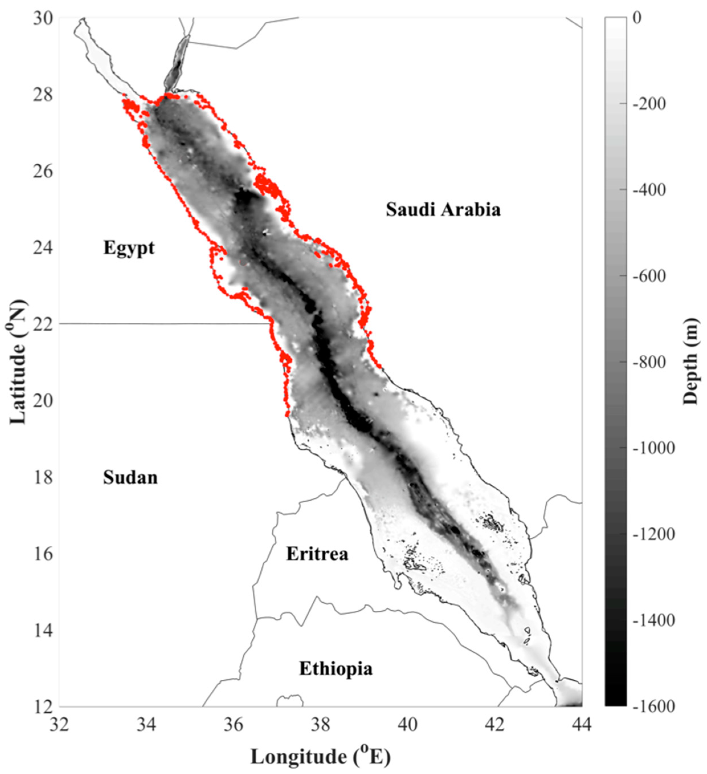
The study region comprises the “northern and central Red Sea”, which occupies an area northwards of ~20°N (Figure 1), separating the northern and southern halves of the Red Sea [47]. Geographical limits of this region were based on the Marine Ecoregions of the World (MEOW) bioregionalisation system led by the World Wildlife Fund and The Nature Conservancy (https://www.worldwildlife.org/publications/marine-ecoregions-of-the-world-a-bioregionalization-of-coastal-and-shelf-areas; www.marineregions.org). This classification system partitions the shelf and coastal regions of the global oceans into “ecoregions”, which are based on a distinct set of oceanographic or topographic characteristics that contribute to areas of homogeneous species composition [48]. We selected this ecoregion as it enabled the acquisition of adequate fisheries landings data needed to provide a more complete view of fisheries dynamics over the northern portion of the Red Sea (see Section 2.5).
2.2. Satellite Ocean Colour Data
Version 4.0 of the European Space Agency’s Ocean Colour Climate Change Initiative (ESA OC-CCI) was used in this study. The OC-CCI product consists of merged and bias-corrected Chl-a data from the Sea-Viewing Wide Field-of-View Sensor (SeaWiFS), Moderate Resolution Imaging Spectroradiometer (MODIS), Medium Resolution Imaging Spectrometer (MERIS), and Visible Infrared Imaging Radiometer Suite (VIIRS) satellite sensors. Level 3, 8-day, mapped Chl-a data were acquired at a spatial resolution of 4 km from http://www.esa-oceancolour-cci.org. We note that for generating high-resolution maps of the satellite-derived fractional contribution of nano/micro-phytoplankton cells (see Figures 4 and 5), we used a Chl-a dataset, produced specifically for the Red Sea at a 1km spatial resolution using the regional algorithm described by Brewin et al. [25]. Brewin et al. [24,25], Racault et al. [28] and Gittings et al. [33,44] have shown that both standard ocean-colour algorithms and the OC-CCI algorithm perform relatively well in the Red Sea, supporting the use of satellite-derived Chl-a datasets. In addition, previous studies in the Red Sea have also demonstrated that the OC-CCI product is characterised by significantly higher data availability in comparison to single-sensor-based missions [28]. For further information, the reader is referred to previous literature regarding the OC-CCI product [49,50,51] and its previous applications in the Red Sea and adjacent Arabian Sea [12,25,26,28,33,44,51]. We also refer the reader to the OC-CCI Product User Guide at http://www.esa-oceancolour-cci.org/?q=webfm_send/318 for a more extensive overview of processing, sensor merging and uncertainty quantification. Observations of Chl-a concentration that were used as inputs for the size model, and the subsequent phenological analysis, were acquired for the northern and central Red Sea ecoregion (as described Section 2.1).
2.3. Two-Component Phytoplankton Size Class Model
For deriving estimates of phytoplankton size structure, we used the two-component model tuned to the Red Sea by Gittings et al. [44]. This conceptual model assumes that small phytoplankton cells (picophytoplankton) do not grow beyond a specific Chl-a concentration, and the addition of more Chl-a into a system, beyond this concentration, can be attributed to that from larger phytoplankton cells [40,52]. The model is based on the exponential equation originally put forth by Sathyendranath et al. [53], and used by Brewin et al. [45] to relate the concentration of Chl-a in pico-phytoplankton (Cp, cells <2 μm in diameter) to the total Chl-a (C) according to
where Cpm is the maximum Chl-a concentration of pico-phytoplankton, and Dp represents the fraction of pico-phytoplankton (Cp/C) as C tends to zero.
Using a High Performance Liquid Chromatography (HPLC) pigment dataset, Gittings et al., (2019b) estimated the model parameters Cpm and Dp for the Red Sea by fitting Equation (1) to in situ estimates of Cp and C. A non-linear, least squares fitting procedure (Trust-Region-Reflective algorithm, MATLAB Optimisation Toolbox, function “LSQCURVEFIT”), in conjunction with bootstrapping [54], was used to compute the parameters and their associated uncertainties. Using this approach, Gittings et al. [44] computed Cpm as 0.19 mg m−3 and Dp as 0.92.
Satellite estimates of Cp were computed using Equation (1) using the Gittings et al. [44] model parameters, and forced with satellite-derived estimates of total Chl-a concentration (C). Chl-a concentrations attributed to the combined nano/micro-phytoplankton assemblage (Cn,m) were then subsequently derived as follows
After deriving Cn,m (from hereafter referred to as large cells), the fractional contribution of this assemblage to total Chl-a (Fn,m) was computed as
The model was run on each grid point, on each of the 8-day CCI mapped Chl-a data products between 1997 and 2018.
2.4. Computation of Phytoplankton Phenology Metrics
Following completion of the time series of Chl-a concentration attributed to large cells (from hereafter referred to as Cn,m), we utilised the cumulative sums of anomalies method, based on a threshold criterion, to estimate the timing of the following phenology metrics: (1) bloom initiation, (2) bloom duration, and (3) bloom termination [12,33,46]. The threshold criterion method is centred on the concept that the occurrence of a phytoplankton bloom corresponds to a significant increase in Chl-a above “normal” concentrations [55]. First, for the estimation of phytoplankton phenology indices, 8-day data corresponding to Cn,m were isolated for the period spanning 29 August 1997–21 August 2018. Cn,m was then spatially-averaged over the northern and central Red Sea ecoregion described in Section 2.1. A moving window filter was then applied to the Cn,m time series (MATLAB subroutine hampel) to remove any outliers. The cumulative sum of anomalies method requires a gap-free Chl-a time-series as an input, otherwise phenology metrics cannot be calculated. Hence, to further improve the coverage of Chl-a satellite data, we applied a linear interpolation method that fills gaps in the time series. The interpolation method used is based on the MATLAB subroutine inpaint_nans, which interpolates missing data using a linear least squares approach [56]. Next, following visual inspection of each annual Cn,m seasonal cycle, we defined the threshold criterion as the long term median of the Cn,m time series, plus 15%. This threshold was selected as it was found to be the most representative of the winter bloom initiation and termination phenology indices for each year over the 21-year period. We note that various thresholds (5%, 10%, and 15%) have been utilised in different Red Sea phenology studies [12,28,33], depending on the type of analysis (e.g., interannual or climatological). Using this threshold, Cn,m anomalies were computed by subtracting the threshold criterion from the time series. The cumulative sums of anomalies were then calculated. Increasing (decreasing) trends in the cumulative sums of anomalies represent periods when Chl-a concentrations are above (below) the threshold criterion. The gradient of the cumulative sums of anomalies was then used to identify the timing of the transition between increasing and decreasing trends. The initiation of the phytoplankton bloom corresponded to the 8-day period when Chl-a concentrations first rose above the threshold criterion (i.e., when the gradient of the time series first changed sign). The termination of the phytoplankton bloom was computed as the time when the gradient first changed sign following the occurrence of the maximum Chl-a concentration in the time series (the growth peak). The total duration of the phytoplankton growth period was calculated as the number of 8-day periods between the timings of initiation and termination.
2.5. Sea Level Anomaly and Geostrophic Velocities
Satellite altimetry can be used to study the circulation dynamics and the propagation of cyclonic and anticyclonic oceanic eddies. We used sea level anomaly (SLA) derived from satellite altimetry, and associated geostrophic velocity data produced by Ssalto/Duacs and distributed by AVISO with support from the Centre National D’Etudes Spatiales (CNES). The geostrophic velocities are computed from gridded sea surface heights with respect to a twenty-year mean (1993–2012), based on multi-mission satellite altimeter observations. Daily data were acquired on a regular 1/4° grid between mid-September and mid-October 2002, and were then averaged into a monthly composite. The full methodological approach, and its application in the nearby Red Sea, can be found in Zhan et al. [57].
2.6. Fisheries Landings Data
We utilised fisheries catch data from the Sea Around Us initiative (University of British Columbia), which is available online at www.seaaroundus.org. Annual data corresponding to the total reported landings of Sardinella spp. (Clupeiformes) and Squid spp. (Teuthida) in the northern and central Red Sea ecoregion (Figure 1) were acquired between 1998 and 2016. We focused on landings data collected for Sardinella spp. and Squid spp. (Teuthida, genus not reported in dataset) to provide examples of pelagic organisms from vertebrate and invertebrate groups, which have a crucial intermediate role in marine food webs (linking plankton and higher predatory fish). Clupeiformes, such as Sardinella spp., are planktivorous and respond strongly to environmental perturbations, particularly changes in food (phytoplankton) availability [58,59]. They are also amongst some of the most significant contributors to fishery catches [60,61]. Similarly, the level of food availability (as indexed by Chl-a concentration) is an essential factor influencing the stock recruitment of juvenile squid, which feed directly on various different types of plankton during their paralarval phases [62,63]. The catch dataset is based on combine official reported data from the Food and Agriculture Organisation of the United Nations (FAO) FishStat database, and reconstructed estimates of unreported catch data. For further information on the reconstruction of fisheries catch data, we refer the reader to and Pauly and Zeller [64]. We note that un-normalized fishery landings do not necessarily represent stock abundance, and fluctuations in these datasets could be also influenced by other factors. However, trends in fisheries stocks are commonly detected by analysing catch or landings per unit of effort, and studies have shown that catch data are consistent with phytoplankton biomass trends [59,65,66].
3. Results
3.1. Interannual Variability of Phenology Anomalies Attributed to Large Phytoplankton
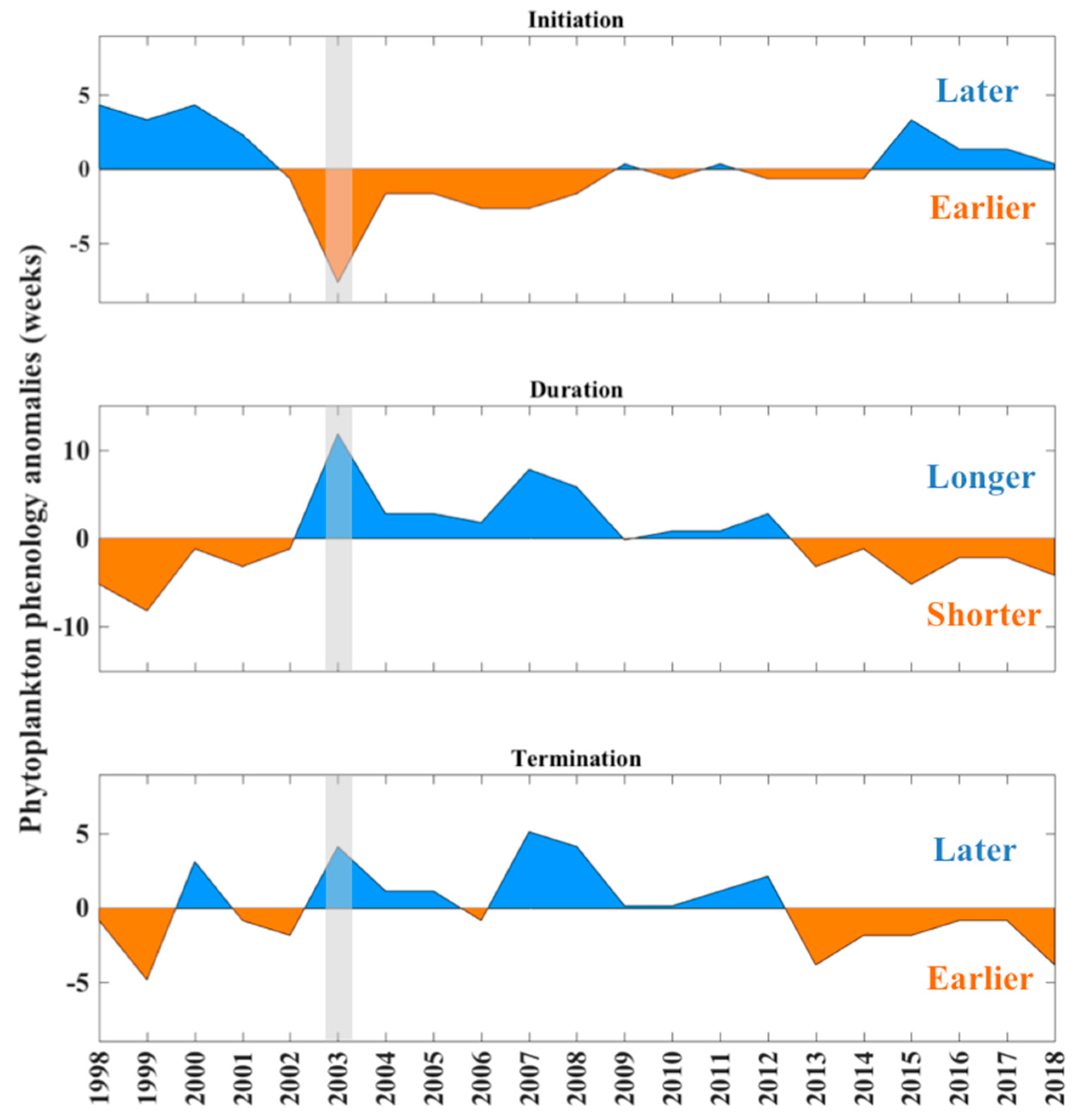
First, we examined the interannual variability of phenology metrics (initiation, duration, and termination) associated with the large phytoplankton assemblage (>2 μm in diameter) for a 21-year period spanning 1998–2018 (Figure 2). The values are presented as annual anomalies, and represent the number of 8-day periods (from hereafter referred to as “weeks” for convenience) above/below the mean timing of growth initiation, duration, and termination. For each phenology metric, distinct positive and negative phases of the annual phenology anomalies can be observed. Between 1998 and 2002, the winter growth period of the nano/micro phytoplankton assemblage initiates later, is shorter in duration and terminates earlier. In particular, 1998 and 1999 are characterised by winter blooms that start between 4 and 5 weeks later. The bloom during 1999 terminates up to ~5 weeks earlier, resulting in a duration (phytoplankton growth period) that is ~9 weeks shorter than average (Figure 2). A substantially earlier initiation can also be observed in 2000 and 2001.
Between 2002 and 2008, the phytoplankton growth periods start earlier, are longer in duration and have a delayed termination. One of the most notable events can be observed in 2003, where the phytoplankton growth period initiates ~8 weeks earlier and terminates ~3 weeks later, resulting in a duration which is ~11 weeks longer than average, and is the longest winter bloom duration observed over the entire 21-year study period (grey shaded bar in Figure 2). Notably longer blooms (~5–6 weeks) are also apparent in 2007 and 2008 and appear to be predominantly driven by a delay in bloom termination (~4–5 weeks). From 2009 to 2018, the annual phenology anomalies either do not show any substantial differences from the average (e.g., between 2009 and 2012) or revert back to the pattern observed between 1998 and 2002, where winter blooms are generally characterised by a delayed initiation (<4 weeks), earlier termination (<4 weeks), and shorter duration (<5 weeks).
3.2. Abundance and Phenology of Large Phytoplankton Associated with the 2003 Winter Bloom
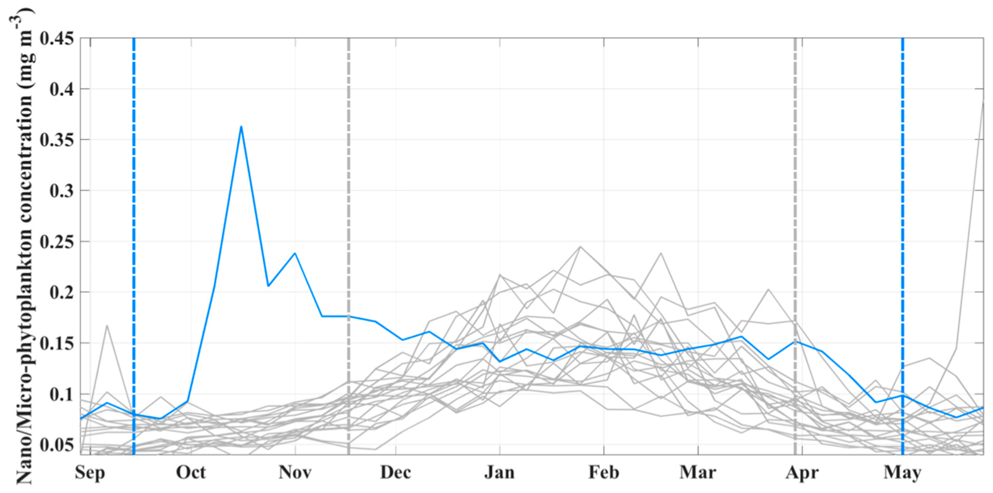
The northern and central Red Sea ecoregion experienced the longest bloom of large phytoplankton during the autumn/winter of 2002/2003 (Figure 2). To further investigate the phenological characteristics of this bloom, as well as the seasonality of Chl-a concentration attributed to large cells (Cn,m), we present time series of Cn,m during the entire autumn/winter period blooming period (September–May) of 2002/2003, alongside the corresponding timings of bloom initiation and termination (highlighted in blue, Figure 3). For comparison, we also highlight the seasonal cycles of Cn,m and phenology metrics for the remaining years of the study period (shown in grey, Figure 3).
Overall, the time series of Cn,m reveals a consistent winter seasonal cycle. Cn,m increases gradually in late-October/early-November, before reaching maximum concentrations of ~0.25 mg m−3 between January and March (grey lines, Figure 3). Cn,m returns to pre-bloom conditions (0.05–0.1 mg m−3) by early/mid-April. In contrast, the time series of Cn,m during the autumn/winter of 2002/2003 (shown in blue) is characterised by a prominent peak in mid-October (~0.36 mg m−3), which is not observed for any of the other years. Cn,m remains above ~0.2 mg m−3 until early-November, when it decreases and stabilises at concentrations that are comparable with the bloom peaks of the other years (~0.15 mg m−3). By May, Cn,m returns to concentrations that were observed prior to the start of the winter bloom (<0.1 mg m−3). Comparing the climatological phenology metrics (grey dashed lines) with those computed independently for the autumn/winter of 2002/2003 (blue dashed lines), further emphasises the markedly earlier bloom initiation of large phytoplankton in mid-September of 2002 (~8 weeks), as well as the delayed termination (~3 weeks) at the beginning of May 2003 (Figure 3).
3.3. Spatial Distribution of the Large Phytoplankton during the Initiation of the 2002/2003 Winter Bloom
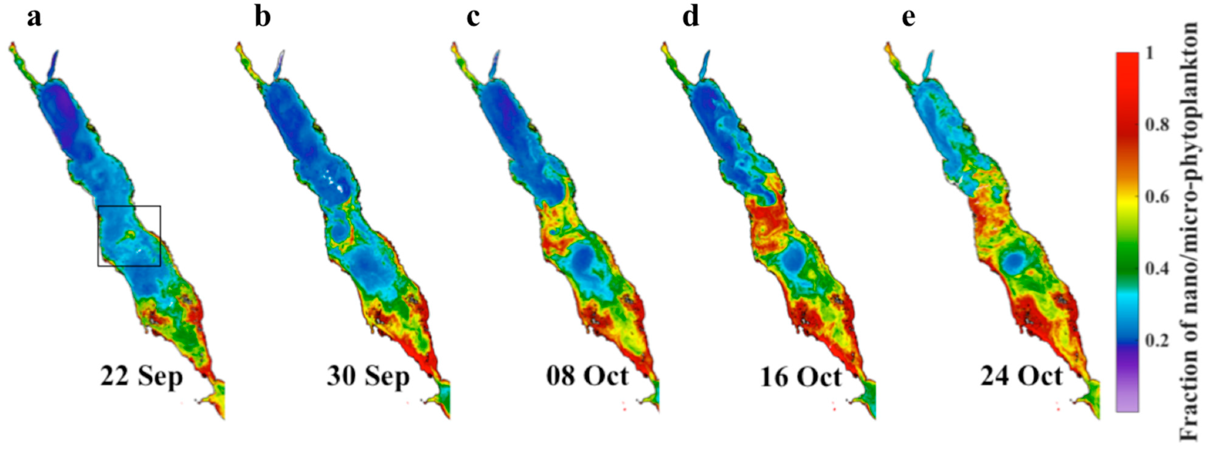
To elucidate the factors contributing to the high abundance of large phytoplankton in October 2002 (Figure 3), we created maps showing the spatial distribution of the satellite-derived fractional contribution of the nano/micro-phytoplankton assemblage (Fn,m) between late-September and late-October (Figure 4). We chose this period in order to fully capture the onset and progression of the event observed in Figure 2 and Figure 3. Following 22 September 2002, a small localised region characterised by a higher fraction of nano/micro-phytoplankton (Fn,m = 0.3–0.6) is apparent in the central Red Sea (black box, Figure 4a). This region is situated closer to the eastern (Arabian) coastline, although waters characterised by a higher fraction of larger cells can be detected extending towards the western (African) coastline. In the week following 30 September, the region develops into mesoscale cyclonic eddy and a higher fraction of larger cells can be observed in its’ periphery (Fn,m > 0.6, Figure 4b). Simultaneously, a mesoscale anticyclonic eddy develops further south, which can be identified as a localised region where there is a reduced fraction of nano/micro-phytoplankton (Fn,m < 0.2, Figure 4b,c). In the weeks following the 8 and 16 October 2002, this eddy dipole intensifies and Fn,m increases considerably in the regions occupied by the upper cyclonic eddy (Fn,m < 0.8) and the convergence zone where the peripheries of the two eddies meet (Figure 4c,d).
A filament of water masses characterised by a larger fraction of nano/micro-phytoplankton (Fn,m = 0.3 − 0.4) appears to be advected from the region of mesoscale eddy activity in the central Red Sea, traveling northwards along the eastern coastline (Figure 4d). From 24 October 2002, a clear enhancement in the fractional contribution of nano/micro-phytoplankton can be observed over the northern and central Red Sea (Fn,m = 0.4 − 0.8), and the pathway of water mass transport follows the eastern coastline of the northern Red Sea. After reaching the northern end of the Red Sea, the water masses rotate westwards along the northernmost boundary and traveling southwards along the northwest coastline (Figure 4e). Higher values of Fn,m can be observed across the majority of the northern and central Red Sea (Figure 4e).
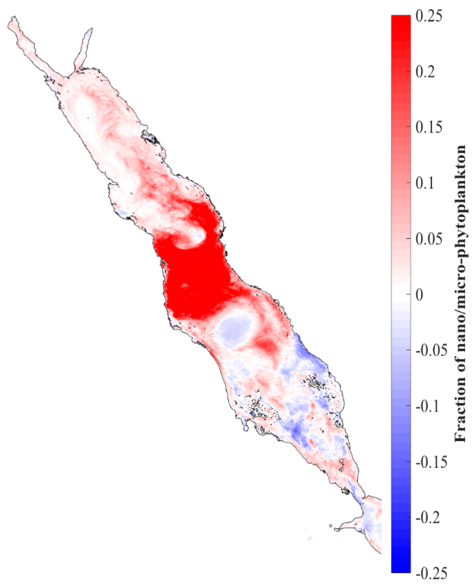
The overall development and progression of this event can also be detected in the monthly anomaly of the fractional contribution of the nano/micro-phytoplankton assemblage for October 2002 (Figure 5). The fraction of nano/micro-phytoplankton is more than 25% higher than average in the central Red Sea (in comparison with all Octobers during 1998–2018), corresponding to the region of strong eddy activity (Figure 4). The advection of water masses characterised by higher fractions of larger cells (Fn,m = 0.05 − 0.15, Figure 4d,e) can also be seen extending northwards from the Central Red Sea along the eastern coastline of the northern Red Sea, towards the northernmost part of the basin.
To further corroborate the observed relationships between regional circulation dynamics and the increase in the abundance of large cells during September/October 2002 (Figure 4 and Figure 5), we generated a monthly composite of sea level anomaly (SLA), representing the period between 15 September and 15 October 2002 (Figure 6). We also present the anomalies of the geostrophic velocities, overlaid on top of the SLA, as represented by the black vector fields. This period was selected in order to highlight circulation patterns during the initiation and peak of the 2002/2003 winter bloom (as seen in Figure 3). The mesoscale eddy dipole in the central Red Sea can clearly be observed in the monthly map, as shown by the counter-clockwise (clockwise) rotating vector fields in the northern (southern) parts of the dipole region (~18N)°. The position of the strong cyclonic eddy also coincides with the region of increased values of Fn,m observed in the central Red Sea (as seen in Figure 4 and Figure 5). A prominent northward flow can be observed along the eastern coastline of the northern and central Red Sea, which is analogous with the apparent northward advection of water masses characterised by larger cells observed in Figure 4 and Figure 5.
3.4. Exploring Potential Links between the 2003 Winter Phytoplankton Bloom and Fisheries
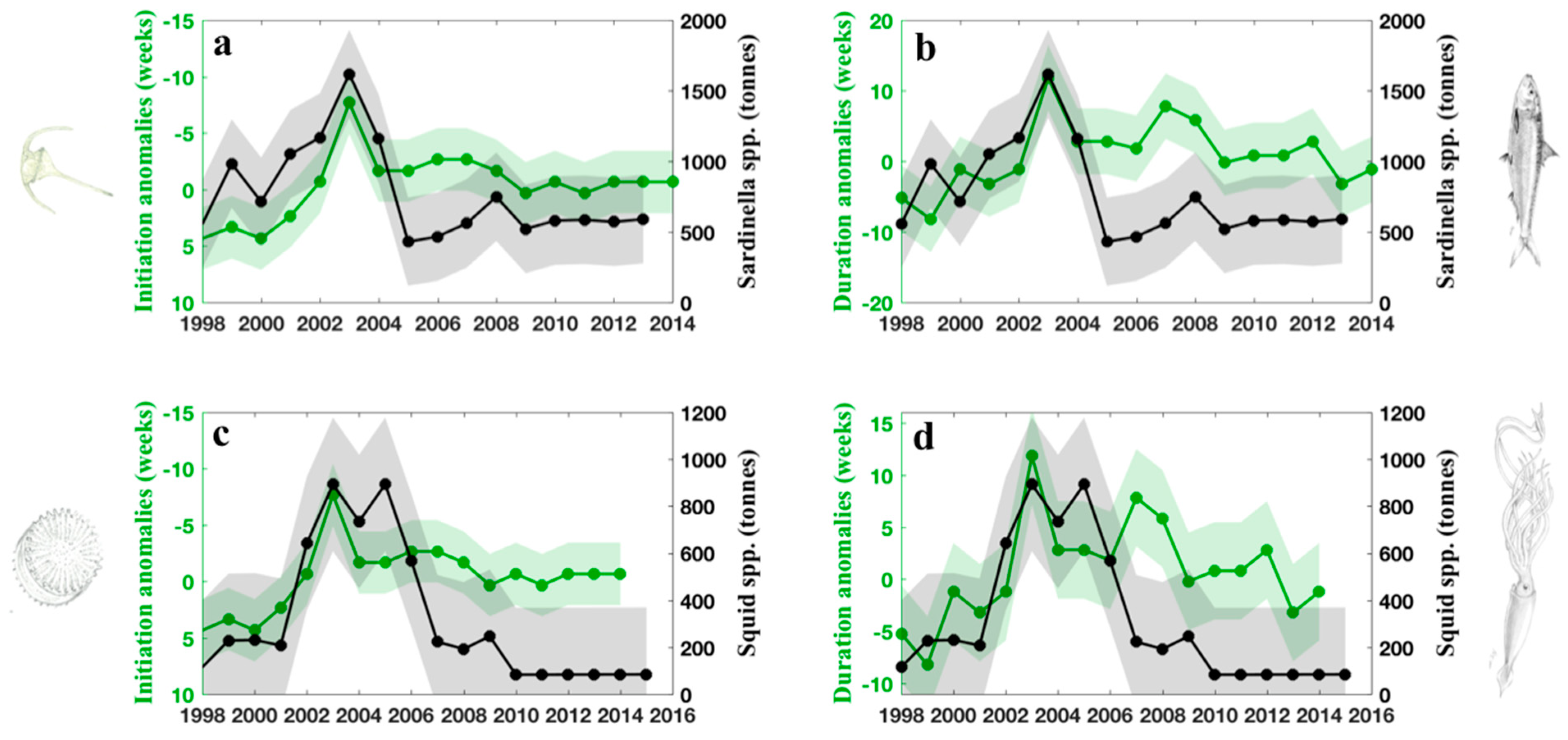
We highlighted the interannual variability of phenological metrics associated with the large phytoplankton assemblage (phytoplankton cells, >2 μm) in the northern and central Red Sea. We subsequently identified a winter bloom that initiated in late September 2002 and subsisted until May 2003—the longest winter bloom duration recorded over the last 20 years (Figure 2 and Figure 3). To put these findings in the context of fisheries, we present time series corresponding to the total landings (tonnes) of two pelagic fisheries groups—Sardinella spp. and Squid spp. (Teuthida, genus not provided) reported in the Northern and Central Red Sea ecoregion for the period spanning 1998–2014 and 1998–2016, respectively (black lines, Figure 7).
In order to investigate the relationship between phenology and fisheries, we also present the interannual anomalies of phytoplankton bloom initiation and bloom duration (highlighted in green) versus the two pelagic fisheries groups (in black, Figure 7). We note that we subtracted one year from the time series of fisheries landings in Figure 7, so the plotted time series actually corresponds to one year after the phytoplankton bloom (year t + 1). This was done because a 1-year lag was identified between phytoplankton phenology metrics and fisheries landings (see Discussion).
Overall, the annual anomalies of the initiation and duration of phytoplankton growth show clear negative and positive relationships with the landings of Sardinella spp., respectively (please note the reversed y-axes in Figure 7a,c). Although the correlations between Sardinella spp. and bloom initiation (r = −0.34, p > 0.05, n = 16) and duration (r = 0.23, p > 0.05, n = 16) (Figure 7a,b) are not significant at 95% level, higher (lower) landings of Sardinella spp. are observed in years when the bloom initiation occurs earlier (later). The maximum catch in Sardinella spp. in year t + 1 (2004) (~1750 tonnes more than the mean annual catch) coincides clearly with the earliest bloom initiation (~8 weeks earlier), and the longest bloom duration (~11 weeks longer), associated with the autumn/winter of 2002/2003 (year t). Significant relationships can be observed between the catch of Squid spp. and the annual anomalies of bloom initiation (r = −0.59, p < 0.05, n =18) and duration (and r = 0.48, p < 0.05, n = 18). The maximum catch of squid in 2004 also coincides with the earliest bloom initiation and longest bloom duration in 2002/2003, and remains higher for the consecutive two years (Figure 7c,d). After this, total landings decrease and fluctuate between 100–250 tonnes for the remainder of the study period.
4. Discussion
Using the phytoplankton size model of Gittings et al. [44], we derived remotely-sensed Chl-a concentrations for large phytoplankton (cells > 2 µm) in the northern and central Red Sea. We then investigated the interannual variability of their phenology metrics (initiation, duration and termination) over a 21-year study period (1998–2018) and explored the ecological implications of our results by linking the observed trends with fisheries dynamics. The annual phenology metrics exhibit fluctuating periods of negative and positive phases (Figure 2). Between 2002 and 2008, winter phytoplankton growth periods of large phytoplankton were generally characterised by an earlier initiation (negative anomaly), delayed termination (positive anomaly), and longer duration (positive anomaly) (Figure 2). These results are generally consistent with the study by Raitsos et al. [11], who revealed that phytoplankton abundance and phenology in the Red Sea vary in conjunction with fluctuating phases of the Multivariate El Niño Southern Oscillation Index (MEI). During positive MEI phases, such as the period between 2002 and 2008 (see Raitsos et al. [11] their Figure 1), southwesterly winds associated with the winter Arabian monsoon intensify over the Southern Red Sea, driving increased horizontal advection of nutrient-rich surface waters from the Indian Ocean (Gulf of Aden). Consequently, winter phytoplankton abundance has been shown to increase by up to 75% in the Red Sea during positive MEI phases and winter growth periods are prolonged by an average of ~2 weeks, primarily due to the earlier initiation of phytoplankton growth [11]. Analogously, the delayed initiation and shorter duration we observed between 1998 and 2002 and 2013–2018, is likely associated with negative MEI (La Niña) phases. During negative MEI, the winter monsoon winds are weakened, driving reduced volume transport of nutrient-rich waters from the Gulf of Aden. This delays the initiation of the winter phytoplankton growth period and reduces its magnitude. We note that the northernmost region of the Red Sea does not emulate this pattern, as phytoplankton dynamics in this region are primarily governed by the strength of winter convective mixing, as typically observed in other tropical marine systems [12,27,28,29,32,33]. Despite the larger study region used in our study, our results are also consistent with Gittings et al. [12], who detected similar patterns of interannual variability in the phenology anomalies of Chl-a in a smaller part of the northern Red Sea (>25.5ºN). Accordingly, the interannual variability of large phytoplankton in the northern and central Red Sea is likely controlled by a combination of the two mechanisms that bring nutrients to the sunlit zone; vertical mixing from convection in the far northern Red Sea, and the horizontal advection of fertile water masses originating from the Gulf of Aden.
One of the most interesting results of our analysis relates to the winter bloom of 2002/2003. The bloom initiation occurred in mid-September 2002—the earliest detected over the 21-year study period (Figure 2 and Figure 3). Cn,m during this year subsequently peaked in mid-October (~0.36 mg m−3), which also constituted the highest winter concentrations of nano/micro-phytoplankton observed over the entire study period (Figure 3). Cn,m remained elevated until the beginning of May 2003, resulting in a phytoplankton bloom that was almost three months longer than the climatological average (Figure 2 and Figure 3). As previously discussed, the MEI transitioned from a negative (La Niña) to positive (El Niño) phase in 2002 (Raitsos et al. [11] their Figure 1). We speculate that the commencement of the winter Arabian monsoon in October 2002, combined with the establishment of an El Niño phase, increased the horizontal advection of nutrient-rich water masses from the Gulf of Aden into the Red Sea, which contributed to: (1) a stronger winter phytoplankton bloom (Figure 3); and (2) a bloom characterised by an earlier initiation and longer duration (Figure 2). However, spatial analysis of this event revealed that the fractional contribution of large phytoplankton increased earlier (towards the end of September), predominantly in the central Red Sea (black box, Figure 4a), and continued to increase throughout October (Figure 4b–e). The horizontal circulation of the Red Sea is known to be influenced by the frequent occurrence of mesoscale eddies, particularly in the central part of the basin [30,57,67,68,69,70,71,72]. Between mid-September and the end of October 2002, we detected a pair of mesoscale eddies in the central Red Sea—a cyclonic eddy in the northern part and an anticyclonic eddy in the southern part of the province (e.g., Figure 4c, Figure 5 and Figure 6). This eddy dipole could be associated with wind jets that blow through the Tokar Gap into the Red Sea, and has been previously reported to occur in the central Red Sea (~19°N) during the summer monsoon (June-September) [73,74,75]. Cyclonic eddies are known to be of biological importance, as they are associated with the upwelling of colder, nutrient-rich waters to the surface layer. One potential source of nutrients could relate to the summer subsurface intrusion of fresher, nutrient-rich Gulf of Aden Intermediate Water (GAIW)). Model simulations and analyses using in situ datasets have demonstrated that GAIW propagates northwards following its intrusion during summer [26,70,76,77,78]. As GAIW moves northwards, mixing between GAIW and the surface waters has the potential to redistribute nutrients to the surface layer, stimulating phytoplankton growth. Hence, the large increase in the concentration/fraction of large phytoplankton in the Central Red Sea could be attributed to increased nutrient availability via upwelling associated with a cyclonic eddy. In accordance with our results, Kurten et al. [79] detected higher Chl-a concentrations attributed to micro-phytoplankton (e.g., diatom spp., such as Thalassiosira subtilis and Pseudo-nitzschia cuspidate) in the central regions of the Red Sea during spring, as a result of cyclonic eddy activity. Similarly, Zarokanellos et al. [80] reported that a cyclonic eddy detected in the central Red Sea during spring was associated with the upward flux of nutrients into the euphotic zone, which contributed to higher Chl-a concentrations.
Aside from vertical mixing processes, mesoscale eddy activity and large-scale circulation features have been shown to facilitate the horizontal exchange of water masses from coastal to offshore waters, as well as to more distant coastal regions. For example, Raitsos et al. [30] demonstrated that mesoscale circulation features, such as anticyclonic eddies, may advect nutrient-rich water masses for distances exceeding 250 km, in less than two weeks, between distant coral reef complexes that line the eastern and western coastline of the Red Sea. These dynamic circulation patterns may further increase nutrient availability and enhance phytoplankton growth in offshore waters (e.g., Figure 4b). In agreement with previous studies, we found evidence of water mass transport from the central region of eddy activity towards the northern Red Sea, along the eastern coastline (Figure 4d,e, Figure 5 and Figure 6). We speculate that this filament, characterised by a higher fraction of large phytoplankton (and most likely higher concentrations of nutrients), can be attributed to the interaction between the cyclonic eddy in the central Red Sea (Figure 4 and Figure 5) and the eastern boundary current in the northern Red Sea [76,81,82].
Our results indicate a direct linkage between the timing of winter blooms of larger phytoplankton cells, and the landings of commercially important fisheries in the northern and central Red Sea. Although the diet of the larvae of Sardinella spp. may be diverse, studies in other oceanic regions have shown that they regularly feed directly upon larger phytoplankton cells (e.g., diatoms), depending on the regional environmental conditions [66,83]. As we cannot confirm the specific species of Sardinella associated with the landings data in our study, it is difficult to know the exact spawning season of the Sardinella spp. analysed in our study. However, the main spawning season of the Indian oil sardine (Sardinella longiceps) has been reported to occur between June and September in the nearby Arabian Sea, coinciding with the summer monsoon [84,85,86]. A similar spawning season (April–September) was reported for Sardinella fimbriata in the Arabian Gulf [87]. Thus, we hypothesise that the positive relationship between the annual timings of bloom initiation/duration, and the catch of Sardinella spp. in the following year, can be explained by a typical match-mismatch scenario [88,89]: in years when the winter bloom initiates earlier (e.g., ~8 weeks in 2002/2003), there is a higher abundance of food (plankton) in the latter stages of the spawning season and Sardinella larva subsequently have enough food to grow and survive during their most vulnerable life stage, leading to enhanced recruitment and a higher catch in the following year. Supporting this, maximum landings of Sardinella spp. were reported in 2004—one year after the 2003 winter bloom (Figure 7). Conversely, when the initiation of bloom is delayed, food availability for Sardinella larva is low and a higher proportion of larvae do not survive. This impacts recruitment success, and consequently, the total catch in the following year. These results agree with Kassi et al. [66], who found that a large portion of the interannual variability observed for the catch of Sardinella aurita in waters of the Ivorian Coast (West Africa) could be attributed to the timing of phytoplankton bloom initiation in the previous year. Additionally, Tzanatos et al. [65] also observed a 1-year lag between the Landings per Unit of Effort (LPUE) of several commercially important fish and squid species and sea surface temperature in the Mediterranean, and proposed that the impacts of warmer conditions, may reduce phytoplankton biomass, and potentially affect fisheries landings in the successive years.
We detected comparable relationships between bloom phenology and the total landings of Squid spp., which are known to be a commercially and economically important fishery in the Red Sea (Figure 7) [90]. Although little is known about the seasonal spawning dynamics of squid in the Red Sea, previous reports indicate that spawning may occur between August–October in the Indian Ocean [91]. Therefore, years characterised by higher landings of Squid spp. may also be attributed to increased food availability and higher recruitment success during the spawning season of the previous year.
5. Conclusions
To the best of our knowledge, the analysis presented in this paper comprises the first attempt to assess the linkages between the interannual variability of satellite-derived ecological indicators and fisheries dynamics in the Red Sea. Using a two-component phytoplankton size class model, re-parameterised for the Red Sea, we derived the Chl-a concentration attributed to large phytoplankton (cells larger than 2 µm) and examined the interannual variability of phenology metrics associated with this partitioned size class.
The phenology of larger phytoplankton size classes in the study region exhibits a interannual variability, which can likely be explained by a combination of two physical mechanisms that are known to influence the concentration of nutrients in the northern and central Red Sea: (1) horizontal advection of nutrient-rich water masses from the Gulf of Aden and redistribution of eddies; and (2) winter convective mixing in the northernmost regions of the Red Sea. We revealed the occurrence of an anomalously long winter phytoplankton bloom in the autumn/winter of 2002/2003, which was characterised by a markedly earlier bloom initiation (~8 weeks earlier than average) and a substantially prolonged duration (~11 weeks longer). Spatial analysis of this event revealed that mesoscale circulation features, predominantly the occurrence of a strong eddy dipole in the central Red Sea, increased nutrient availability that enhanced the growth of large phytoplankton across the broader northern and central Red Sea. We stress that the timing of food availability may directly impact the recruitment success of higher trophic levels, as represented by the maximum catch of two commercially important fisheries (Sardinella spp. and Teuthida) in the year following the blooming event of 2002/2003.
In regions where in situ datasets are scarce, satellite-derived ecological indicators are likely to become essential for understanding the large-scale trophic dynamics of marine ecosystems. The observed linkages between satellite-derived phytoplankton phenology metrics and fisheries may serve as an early “warning system” [92] where an anomalous alteration to bloom timing is an indication that the landings of commercially important species may be impacted in the following year. This is important for policy makers who are responsible for the development and implementation of ecosystem management strategies.
Author Contributions
Conceptualization: J.A.G., D.E.R., R.J.W.B., and I.H.; methodology: J.A.G., D.E.R., and R.J.W.B; software: J.A.G.; validation: J.A.G.; formal analysis: J.A.G., D.E.R., and R.J.W.B.; writing—original draft preparation: J.A.G.; writing—review and editing: J.A.G., D.E.R., R.J.W.B., and I.H.; data curation: J.A.G.; supervision, D.E.R. and I.H; project administration, I.H.; funding acquisition: I.H. All authors have read and agreed to the published version of the manuscript.
Funding
This research was funded by the Office of Sponsored Research (OSR) at King Abdullah University of Science and Technology (KAUST) under the Virtual Red Sea Initiative (Grant #REP/1/3268-01-01), the Center of Excellence NEOM at KAUST, and the BICEP project (European Space Agency).
Institutional Review Board Statement
Not applicable.
Informed Consent Statement
Not applicable.
Data Availability Statement
Publicly available datasets were analysed in this study.
Acknowledgments
The authors are grateful to the Ocean Colour CCI team (European Space Agency) for providing and processing the Chl-a dataset. The authors would also like to thank George Krokos and Larissa Patricio Valerio for their useful discussions. The authors are also grateful to Peng Zhan for kindly providing the sea level anomaly and geostrophic velocity data. The authors also thank Vasiliki Siafaka for providing the sketches of Sardinella spp. and Squid spp. included in Figure 7 of this manuscript.
Conflicts of Interest
The authors declare no conflict of interest.
References
- Berumen, M.L.; Hoey, A.S.; Bass, W.H.; Bouwmeester, J.; Catania, D.; Cochran, J.E.M.; Khalil, M.T.; Miyake, S.; Mughal, M.R.; Spaet, J.L.Y.; et al. The status of coral reef ecology research in the Red Sea. Coral Reefs 2013, 32, 737–748. [Google Scholar] [CrossRef]
- Moberg, F.; Folke, C. Ecological goods and services of coral reef ecosystems. Ecol. Econ. 1999, 29, 215–233. [Google Scholar] [CrossRef]
- Gladstone, W.; Curley, B.; Shokri, M.R. Environmental impacts of tourism in the Gulf and the Red Sea. Mar. Pollut. Bull. 2013, 72, 375–388. [Google Scholar] [CrossRef] [PubMed]
- Carvalho, S.; Kürten, B.; Krokos, G.; Hoteit, I.; Ellis, J. The Red Sea. World Seas An Environ. Eval. Vol. II Indian Ocean to Pacific; Academic Press: Cambridge, MA, USA, 2018; pp. 49–74. [Google Scholar] [CrossRef]
- Raitsos, D.E.; Hoteit, I.; Prihartato, P.K.; Chronis, T.; Triantafyllou, G.; Abualnaja, Y. Abrupt warming of the Red Sea. Geophys. Res. Lett. 2011, 38, 1–5. [Google Scholar] [CrossRef] [Green Version]
- Chaidez, V.; Dreano, D.; Agusti, S.; Duarte, C.M.; Hoteit, I. Decadal trends in Red Sea maximum surface temperature. Sci. Rep. 2017, 1–8. [Google Scholar] [CrossRef] [Green Version]
- Krokos, G.; Papadopoulos, V.P.; Sofianos, S.S.; Ombao, H.; Dybczak, P.; Hoteit, I. Natural Climate Oscillations may Counteract Red Sea Warming Over the Coming Decades. Geophys. Res. Lett. 2019, 46, 3454–3461. [Google Scholar] [CrossRef] [Green Version]
- Monroe, A.A.; Ziegler, M.; Roik, A.; Röthig, T.; Hardenstine, R.S.; Emms, M.A.; Jensen, T.; Voolstra, C.R.; Berumen, M.L. In situ observations of coral bleaching in the central Saudi Arabian Red Sea during the 2015/2016 global coral bleaching event. PLoS ONE 2018, 13, e0195814. [Google Scholar] [CrossRef]
- Osman, E.O.; Smith, D.J.; Ziegler, M.; Kürten, B.; Conrad, C.; El-Haddad, K.M.; Voolstra, C.R.; Suggett, D.J. Thermal refugia against coral bleaching throughout the northern Red Sea. Glob. Chang. Biol. 2018, 24, e474–e484. [Google Scholar] [CrossRef]
- Genevier, L.G.C.; Jamil, T.; Raitsos, D.E.; Krokos, G.; Hoteit, I. Marine heatwaves reveal coral reef zones susceptible to bleaching in the Red Sea. Glob. Chang. Biol. 2019, 25, 2338–2351. [Google Scholar] [CrossRef] [Green Version]
- Raitsos, D.E.; Yi, X.; Platt, T.; Racault, M.F.; Brewin, R.J.W.; Pradhan, Y.; Papadopoulos, V.P.; Sathyendranath, S.; Hoteit, I. Monsoon oscillations regulate fertility of the Red Sea. Geophys. Res. Lett. 2015, 42, 855–862. [Google Scholar] [CrossRef] [Green Version]
- Gittings, J.A.; Raitsos, D.E.; Krokos, G.; Hoteit, I. Impacts of warming on phytoplankton abundance and phenology in a typical tropical marine ecosystem. Sci. Rep. 2018, 8, 2240. [Google Scholar] [CrossRef] [PubMed]
- Brewin, R.J.W.; Morán, X.A.G.; Raitsos, D.E.; Gittings, J.A.; Calleja, M.L.; Viegas, M.; Ansari, M.I.; Al-Otaibi, N.; Huete-Stauffer, T.M.; Hoteit, I. Factors Regulating the Relationship Between Total and Size-Fractionated Chlorophyll-a in Coastal Waters of the Red Sea. Front. Microbiol. 2019, 10, 1964. [Google Scholar] [CrossRef] [PubMed]
- Silva, L.; Calleja, M.L.; Huete-Stauffer, T.M.; Ivetic, S.; Ansari, M.I.; Viegas, M.; Morán, X.A.G. Low Abundances but High Growth Rates of Coastal Heterotrophic Bacteria in the Red Sea. Front. Microbiol. 2019, 9, 3244. [Google Scholar] [CrossRef] [PubMed] [Green Version]
- Hoteit, I.; Abualnaja, Y.; Afzal, S.; Ait-El-Fquih, B.; Akylas, T.; Antony, C.; Dawson, C.; Asfahani, K.; Brewin, R.J.; Cavaleri, L. Towards an End-to-End Analysis and Prediction System for Weather, Climate, and Marine Applications in the Red Sea. Bull. Am. Meteorol. Soc. 2020, 1–61. [Google Scholar] [CrossRef]
- Pelling, M.; Blackburn, S. Megacities and the Coast: Risk, Resilience and Transformation.; Routledge: Oxfordshire, UK, 2014; ISBN 1135074755. [Google Scholar]
- Sekovski, I.; Newton, A.; Dennison, W.C. Megacities in the coastal zone: Using a driver-pressure-state-impact-response framework to address complex environmental problems. Estuar. Coast. Shelf Sci. 2012, 96, 48–59. [Google Scholar] [CrossRef]
- Platt, T.; Sathyendranath, S. Ecological indicators for the pelagic zone of the ocean from remote sensing. Remote Sens. Environ. 2008, 112, 3426–3436. [Google Scholar] [CrossRef]
- Racault, M.F.; Platt, T.; Sathyendranath, S.; Aǧirbaş, E.; Martinez Vicente, V.; Brewin, R. Plankton indicators and ocean observing systems: Support to the marine ecosystem state assessment. J. Plankton Res. 2014, 36, 621–629. [Google Scholar] [CrossRef] [Green Version]
- Smith, S.V.; Hollibaugh, J.T. Coastal metabolism and the oceanic organic carbon balance. Rev. Geophys. 1993, 31, 75–89. [Google Scholar] [CrossRef]
- Chassot, E.; Bonhommeau, S.; Dulvy, N.K.; Mélin, F.; Watson, R.; Gascuel, D.; Le Pape, O. Global marine primary production constrains fisheries catches. Ecol. Lett. 2010, 13, 495–505. [Google Scholar] [CrossRef]
- Lo-Yat, A.; Simpson, S.D.; Meekan, M.; Lecchini, D.; Martinez, E.; Galzin, R. Extreme climatic events reduce ocean productivity and larval supply in a tropical reef ecosystem. Glob. Chang. Biol. 2011, 17, 1695–1702. [Google Scholar] [CrossRef]
- Platt, T.; White, G.N.; Zhai, L.; Sathyendranath, S.; Roy, S. The phenology of phytoplankton blooms: Ecosystem indicators from remote sensing. Ecol. Modell. 2009, 220, 3057–3069. [Google Scholar] [CrossRef]
- Brewin, R.J.W.; Raitsos, D.E.; Pradhan, Y.; Hoteit, I. Comparison of chlorophyll in the Red Sea derived from MODIS-Aqua and in vivo fluorescence. Remote Sens. Environ. 2013, 136, 218–224. [Google Scholar] [CrossRef]
- Brewin, R.J.W.; Raitsos, D.E.; Dall’Olmo, G.; Zarokanellos, N.; Jackson, T.; Racault, M.F.; Boss, E.S.; Sathyendranath, S.; Jones, B.H.; Hoteit, I. Regional ocean-colour chlorophyll algorithms for the Red Sea. Remote Sens. Environ. 2015, 165, 64–85. [Google Scholar] [CrossRef] [Green Version]
- Dreano, D.; Raitsos, D.E.; Gittings, J.; Krokos, G.; Hoteit, I. The gulf of aden intermediate water intrusion regulates the southern Red Sea summer phytoplankton blooms. PLoS ONE 2016, 11, e0168440. [Google Scholar] [CrossRef] [PubMed] [Green Version]
- Papadopoulos, V.P.; Zhan, P.; Sofianos, S.S.; Raitsos, D.E.; Qurban, M.; Abualnaja, Y.; Bower, A.; Kontoyiannis, H.; Pavlidou, A.; Asharaf, T.T.M.; et al. Factors governing the deep ventilation of the Red Sea. J. Geophys. Res. Ocean. 2015, 1152–1172. [Google Scholar] [CrossRef]
- Racault, M.F.; Raitsos, D.E.; Berumen, M.L.; Brewin, R.J.W.; Platt, T.; Sathyendranath, S.; Hoteit, I. Phytoplankton phenology indices in coral reef ecosystems: Application to ocean-color observations in the Red Sea. Remote Sens. Environ. 2015, 160, 222–234. [Google Scholar] [CrossRef] [Green Version]
- Raitsos, D.E.; Pradhan, Y.; Brewin, R.J.W.; Stenchikov, G.; Hoteit, I. Remote Sensing the Phytoplankton Seasonal Succession of the Red Sea. PLoS ONE 2013, 8, e64909. [Google Scholar] [CrossRef] [Green Version]
- Raitsos, D.E.; Brewin, R.J.W.; Zhan, P.; Dreano, D.; Pradhan, Y.; Nanninga, G.B.; Hoteit, I. Sensing coral reef connectivity pathways from space. Sci. Rep. 2017, 7, 9338. [Google Scholar] [CrossRef] [Green Version]
- Triantafyllou, G.; Yao, F.; Petihakis, G.; Tsiaras, K.P.; Raitsos, D.E.; Hoteit, I. Exploring the Red Sea seasonal ecosystem functioning using a three-dimensional biophysical model. J. Geophys. Res. Ocean. 2014, 119, 1791–1811. [Google Scholar] [CrossRef] [Green Version]
- Acker, J.; Leptoukh, G.; Shen, S.; Zhu, T.; Kempler, S. Remotely-sensed chlorophyll a observations of the northern Red Sea indicate seasonal variability and influence of coastal reefs. J. Mar. Syst. 2008, 69, 191–204. [Google Scholar] [CrossRef]
- Gittings, J.A.; Raitsos, D.E.; Kheireddine, M.; Racault, M.-F.; Claustre, H.; Hoteit, I. Evaluating tropical phytoplankton phenology metrics using contemporary tools. Sci. Rep. 2019, 9, 674. [Google Scholar] [CrossRef] [PubMed]
- Ismael, A.A. Phytoplankton of the Red Sea; Springer: Berlin/Heidelberg, Germany, 2015; pp. 567–583. [Google Scholar]
- Pearman, J.K.; Kürten, S.; Sarma, Y.V.B.; Jones, B.H.; Carvalho, S. Biodiversity patterns of plankton assemblages at the extremes of the Red Sea. FEMS Microbiol. Ecol. 2016, 92, 1–13. [Google Scholar] [CrossRef] [PubMed] [Green Version]
- Kheireddine, M.; Ouhssain, M.; Claustre, H.; Uitz, J.; Gentili, B.; Jones, B.H. Assessing pigment-based phytoplankton community distributions in the Red Sea. Front. Mar. Sci. 2017, 4, 132. [Google Scholar] [CrossRef] [Green Version]
- Jin, P.; Agustí, S. Fast adaptation of tropical diatoms to increased warming with trade-offs. Sci. Rep. 2018, 8, 17771. [Google Scholar] [CrossRef] [Green Version]
- Marañón, E.; Cermeño, P.; Latasa, M.; Tadonléké, R.D. Resource supply alone explains the variability of marine phytoplankton size structure. Limnol. Oceanogr. 2015, 60, 1848–1854. [Google Scholar] [CrossRef] [Green Version]
- Smetacek, V. Diatoms and the silicate factor. Nature 1998, 391, 224–225. [Google Scholar] [CrossRef]
- Chisholm, S.W. Phytoplankton Size. In Primary Productivity and Biogeochemical Cycles in the Sea; Springer US: Boston, MA, USA, 1992; pp. 213–237. [Google Scholar]
- Cotner, J.B.; Biddanda, B.A. Small players, large role: Microbial influence on biogeochemical processes in pelagic aquatic ecosystems. Ecosystems 2002, 5, 105–121. [Google Scholar] [CrossRef]
- Salgado-Hernanz, P.M.; Racault, M.-F.; Font-Muñoz, J.S.; Basterretxea, G. Trends in phytoplankton phenology in the Mediterranean Sea based on ocean-colour remote sensing. Remote Sens. Environ. 2019, 221, 50–64. [Google Scholar] [CrossRef]
- Jin, D.; Kite-Powell, H.; Hoagl, P.; Solow, A. A bioeconomic analysis of traditional fisheries in the Red Sea. Mar. Resour. Econ. 2012, 27, 137–148. [Google Scholar] [CrossRef]
- Gittings, J.A.; Brewin, R.J.W.; Raitsos, D.E.; Kheireddine, M.; Ouhssain, M.; Jones, B.H.; Hoteit, I. Remotely sensing phytoplankton size structure in the Red Sea. Remote Sens. Environ. 2019, 234, 111387. [Google Scholar] [CrossRef]
- Brewin, R.J.W.; Sathyendranath, S.; Hirata, T.; Lavender, S.J.; Barciela, R.M.; Hardman-Mountford, N.J. A three-component model of phytoplankton size class for the Atlantic Ocean. Ecol. Modell. 2010, 221, 1472–1483. [Google Scholar] [CrossRef]
- Racault, M.F.; Le Quéré, C.; Buitenhuis, E.; Sathyendranath, S.; Platt, T. Phytoplankton phenology in the global ocean. Ecol. Indic. 2012, 14, 152–163. [Google Scholar] [CrossRef]
- Berumen, M.L.; Voolstra, C.R.; Daffonchio, D.; Agusti, S.; Aranda, M.; Irigoien, X.; Jones, B.H.; Morán, X.A.G.; Duarte, C.M. The Red Sea: Environmental Gradients Shape a Natural Laboratory in a Nascent Ocean. In Coral Reefs of the Red Sea; Voolstra, C.R., Berumen, M.L., Eds.; Springer: FL, USA, 2019; pp. 1–10. [Google Scholar]
- Spalding, M.D.; Fox, H.E.; Allen, G.R.; Davidson, N.; Ferdaña, Z.A.; Finlayson, M.; Halpern, B.S.; Jorge, M.A.; Lombana, A.; Lourie, S.A.; et al. Marine ecoregions of the world: A bioregionalization of coastal and shelf areas. Bioscience 2007, 57, 573–583. [Google Scholar] [CrossRef] [Green Version]
- Sathyendranath, S.; Brewin, B.; Mueller, D.; Doerffer, R.; Krasemann, H.; Melin, F.; Brockmann, C.; Fomferra, N.; Peters, M.; Grant, M.; et al. Ocean Colour Climate Change Initiative—Approach and initial results. In Proceedings of the 2012 IEEE International Geoscience and Remote Sensing Symposium, Munich, Germany, 22–27 July 2012; pp. 2024–2027. [Google Scholar]
- Sathyendranath, S.; Brewin, R.J.W.; Brockmann, C.; Brotas, V.; Calton, B.; Chuprin, A.; Cipollini, P.; Couto, A.B.; Dingle, J.; Doerffer, R. An ocean-colour time series for use in climate studies: The experience of the ocean-colour climate change initiative (OC-CCI). Sensors 2019, 19, 4285. [Google Scholar] [CrossRef] [Green Version]
- Gittings, J.A.; Raitsos, D.E.; Racault, M.; Brewin, R.J.W.; Pradhan, Y.; Sathyendranath, S.; Platt, T. Remote Sensing of Environment Seasonal phytoplankton blooms in the Gulf of Aden revealed by remote sensing. Remote Sens. Environ. 2017, 189, 56–66. [Google Scholar] [CrossRef] [Green Version]
- Raimbault, P. Size fractionation of phytoplankton in the Ligurian Sea and the Algerian Basin (Mediterranean Sea): Size distribution versus total concentration. Mar. Microb. Food Webs 1988, 3, 1–7. [Google Scholar]
- Sathyendranath, S.; Cota, G.; Stuart, V.; Maass, H.; Platt, T. Remote sensing of phytoplankton pigments: A comparison of empirical and theoretical approaches. Int. J. Remote Sens. 2001, 22, 249–273. [Google Scholar] [CrossRef]
- Efron, B. Bootstrap Methods: Another Look at the Jackknife; Springer: New York, NY, USA, 1992; pp. 569–593. [Google Scholar]
- Siegel, D.A.; Doney, S.C.; Yoder, J.A. The North Atlantic spring phytoplankton bloom and Sverdrup’s critical depth hypothesis. Science 2002, 296, 730–733. [Google Scholar] [CrossRef]
- D’Errico, J. Interpolate NaN Elements in a 2D Array Using Non-NaN Elements. MATLAB Cent. File Exch. Available online: http//www.mathworks.com/matlabcentral/fileexchange/4551-inpaint-nans (accessed on 1 August 2020).
- Zhan, P.; Subramanian, A.C.; Yao, F.; Hoteit, I. Eddies in the Red Sea: A statistical and dynamical study. J. Geophys. Res. Ocean. 2014, 119, 8336–8356. [Google Scholar] [CrossRef] [Green Version]
- Giannoulaki, M.; Schismenou, E.; Pyrounaki, M.-M.; Tsagarakis, K. Habitat characterization and migrations. In Biology and Ecology of Sardines and Anchovies; Taylor and Francis Group: London, UK, 2014; pp. 191–241. [Google Scholar]
- Jebri, F.; Jacobs, Z.L.; Raitsos, D.E.; Srokosz, M.; Painter, S.C.; Kelly, S.; Roberts, M.J.; Scott, L.; Taylor, S.F.W.; Palmer, M.; et al. Interannual monsoon wind variability as a key driver of East African small pelagic fisheries. Sci. Rep. 2020, 10, 1–15. [Google Scholar] [CrossRef]
- Hall, S.J. Effects of Fishing on Marine Ecosystems and Communities; Blackwell Science: Oxford, UK, 1999; ISBN 0632041129. [Google Scholar]
- Duarte, L.O.; García, C.B. Trophic role of small pelagic fishes in a tropical upwelling ecosystem. Ecol. Modell. 2004, 172, 323–338. [Google Scholar] [CrossRef]
- Ichii, T.; Mahapatra, K.; Sakai, M.; Wakabayashi, T.; Okamura, H.; Igarashi, H.; Inagake, D.; Okada, Y. Changes in abundance of the neon flying squid Ommastrephes bartramii in relation to climate change in the central North Pacific Ocean. Mar. Ecol. Prog. Ser. 2011, 441, 151–164. [Google Scholar] [CrossRef] [Green Version]
- Nishikawa, H.; Igarashi, H.; Ishikawa, Y.; Sakai, M.; Kato, Y.; Ebina, M.; Usui, N.; Kamachi, M.; Awaji, T. Impact of paralarvae and juveniles feeding environment on the neon flying squid (Ommastrephes bartramii) winter-spring cohort stock. Fish. Oceanogr. 2014, 23, 289–303. [Google Scholar] [CrossRef]
- Pauly, D.; Zeller, D. Catch reconstructions reveal that global marine fisheries catches are higher than reported and declining. Nat. Commun. 2016, 7. [Google Scholar] [CrossRef] [PubMed]
- Tzanatos, E.; Raitsos, D.E.; Triantafyllou, G.; Somarakis, S.; Tsonis, A.A. Indications of a climate effect on Mediterranean fisheries. Clim. Change 2014, 122, 41–54. [Google Scholar] [CrossRef]
- Kassi, J.B.; Racault, M.F.; Mobio, B.A.; Platt, T.; Sathyendranath, S.; Raitsos, D.E.; Affian, K. Remotely sensing the biophysical drivers of Sardinella aurita variability in Ivorian waters. Remote Sens. 2018, 10, 785. [Google Scholar] [CrossRef] [Green Version]
- Morcos, S.A. Physical and chemical oceanography of the Red Sea. Oceanogr. Mar. Biol. Annu. Rev 1970, 8, 202. [Google Scholar]
- Quadfasel, D.; Baudner, H. Gyre-scale circulation cells in the Red-Sea. Oceanol. Acta 1993, 16, 221–229. [Google Scholar]
- Clifford, M.; Horton, C.; Schmitz, J.; Kantha, L.H. An oceanographic nowcast/forecast system for the Red Sea. J. Geophys. Res. Ocean. 1997, 102, 25101–25122. [Google Scholar] [CrossRef] [Green Version]
- Sofianos, S.S.; Johns, W.E. Observations of the summer Red Sea circulation. J. Geophys. Res. Ocean. 2007, 112, 1–20. [Google Scholar] [CrossRef]
- Zhan, P.; Krokos, G.; Guo, D.; Hoteit, I. Three-Dimensional Signature of the Red Sea Eddies and Eddy-Induced Transport. Geophys. Res. Lett. 2019, 46, 2167–2177. [Google Scholar] [CrossRef] [Green Version]
- Zhan, P.; Subramanian, A.C.; Yao, F.; Kartadikaria, A.R.; Guo, D.; Hoteit, I. The eddy kinetic energy budget in the Red Sea. J. Geophys. Res. Ocean. 2016, 121, 4732–4747. [Google Scholar] [CrossRef] [Green Version]
- Zhai, P.; Bower, A. The response of the Red Sea to a strong wind jet near the Tokar Gap in summer. J. Geophys. Res. Ocean. 2013, 118, 421–434. [Google Scholar] [CrossRef]
- Bower, A.S.; Farrar, J.T. Air–Sea Interaction and Horizontal Circulation in the Red Sea; Springer: Berlin/Heidelberg, Germany, 2015; pp. 329–342. [Google Scholar] [CrossRef]
- Farley Nicholls, J.; Toumi, R.; Stenchikov, G. Effects of unsteady mountain-gap winds on eddies in the Red Sea. Atmos. Sci. Lett. 2015, 16, 279–284. [Google Scholar] [CrossRef] [Green Version]
- Sofianos, S.S. An Oceanic General Circulation Model (OGCM) investigation of the Red Sea circulation: 2. Three-dimensional circulation in the Red Sea. J. Geophys. Res. 2003, 108, 1–15. [Google Scholar] [CrossRef] [Green Version]
- Churchill, J.H.; Bower, A.S.; McCorkle, D.C.; Abualnaja, Y. The transport of nutrient-rich Indian ocean water through the red sea and into coastal reef systems. J. Mar. Res. 2015, 72, 165–181. [Google Scholar] [CrossRef]
- Yao, F.; Hoteit, I.; Pratt, L.J.; Bower, A.S.; Zhai, P.; Köhl, A.; Gopalakrishnan, G. Seasonal overturning circulation in the Red Sea: 1. Model validation and summer circulation. J. Geophys. Res. Ocean. 2014, 119, 2238–2262. [Google Scholar] [CrossRef] [Green Version]
- Kürten, B.; Zarokanellos, N.D.; Devassy, R.P.; El-Sherbiny, M.M.; Struck, U.; Capone, D.G.; Schulz, I.K.; Al-Aidaroos, A.M.; Irigoien, X.; Jones, B.H. Seasonal modulation of mesoscale processes alters nutrient availability and plankton communities in the Red Sea. Prog. Oceanogr. 2019, 173, 238–255. [Google Scholar] [CrossRef]
- Zarokanellos, N.D.; Kürten, B.; Churchill, J.H.; Roder, C.; Voolstra, C.R.; Abualnaja, Y.; Jones, B.H. Physical Mechanisms Routing Nutrients in the Central Red Sea. J. Geophys. Res. Ocean. 2017, 122, 9032–9046. [Google Scholar] [CrossRef] [Green Version]
- Yao, F.; Hoteit, I.; Pratt, L.J.; Bower, A.S.; Köhl, A.; Gopalakrishnan, G.; Rivas, D. Seasonal overturning circulation in the Red Sea: 2. Winter circulation. J. Geophys. Res. Ocean. 2014, 119, 2263–2289. [Google Scholar] [CrossRef] [Green Version]
- Zhai, P.; Pratt, L.J.; Bower, A. On the crossover of boundary currents in an idealized model of the red sea. J. Phys. Oceanogr. 2015, 45, 1410–1425. [Google Scholar] [CrossRef]
- Nieland, H. The food of Sardinella aurita (Val.) and Sardinella eba (Val.) off the coast of Senega. In Proceedings of the The Canary Current: Studies of an Upwelling System. A Symposium; Rapports et Procès-Verbaux des Réunions du Conseil International pour l’Exploration de la Mer: Las Palmas, Spain, 1982; Volume 180, pp. 369–373. [Google Scholar]
- Jayaprakash, A.A.; Pillai, N.G.K. The Indian oil sardine. In Marine Fisheries Research and Management; Pillai, V.N., Menon, N.G., Eds.; CMFRI: Cochin, Kerala, India, 2000; pp. 259–281. [Google Scholar]
- Al-Anbouri, I.S.; Ambak, M.A.; Haleem, S.Z.A. Spawning pattern of Indian oil sardine, Sardinella longiceps Valenciennes, 1847 of Oman Sea, Muscat, Sultanate of Oman. J. Fish. 2013, 7, 72. [Google Scholar] [CrossRef]
- Kripa, V.; Mohamed, K.S.; Koya, K.P.S.; Jeyabaskaran, R.; Prema, D.; Padua, S.; Kuriakose, S.; Anilkumar, P.S.; Nair, P.G.; Ambrose, T.V.; et al. Overfishing and climate drives changes in biology and recruitment of the Indian oil sardine Sardinella longiceps in southeastern Arabian Sea. Front. Mar. Sci. 2018, 5, 1–20. [Google Scholar] [CrossRef] [Green Version]
- Almatar, S.M.; Houde, E.D. Distribution and abundance of sardine Sardinella fimbriata (Val.) eggs in Kuwait waters of the Arabian Gulf. Fish. Res. 1986, 4, 331–342. [Google Scholar] [CrossRef]
- Cushing, D.H. The Possible Density-Dependence of Larval Mortality and Adult Mortality in Fishes. In The Early Life History of Fish; Springer: Berlin/Heidelberg, Germany, 1974; pp. 103–111. [Google Scholar]
- Platt, T.; Fuentes-Yaco, C.; Frank, K.T. Spring algal bloom and larval fish survival. Nature 2003, 423, 398–399. [Google Scholar] [CrossRef] [PubMed]
- Sabrah, M.M.; El-Sayed, A.Y.; El-Ganiny, A.A. Fishery and population characteristics of the Indian squids Loligo duvauceli Orbigny, 1848 from trawl survey along the north-west Red Sea. Egypt. J. Aquat. Res. 2015, 41, 279–285. [Google Scholar] [CrossRef] [Green Version]
- Silas, E.G.; Rao, K.S.; Sarvesan, R.; Nair, K.P.; Meiyappan, M.M. The exploited squid and cuttlefish resources of India: A review. Mar. Fish. Inf. Serv. Tech. Ext. Ser. 1982, 34, 1–16. [Google Scholar]
- Jacobs, Z.L.; Jebri, F.; Srokosz, M.; Raitsos, D.E.; Painter, S.C.; Nencioli, F.; Osuka, K.; Samoilys, M.; Sauer, W.; Roberts, M. A major ecosystem shift in coastal East African waters during the 1997/98 Super El Niño as detected using remote sensing data. Remote Sens. 2020, 12, 3127. [Google Scholar] [CrossRef]
Figure 1.
Map displaying the bathymetry of the Red Sea and geographical location of the northern and central Red Sea ecoregion (limits of this region are highlighted in red). The map was produced using the software package MATLAB (version R2016b).
Figure 1.
Map displaying the bathymetry of the Red Sea and geographical location of the northern and central Red Sea ecoregion (limits of this region are highlighted in red). The map was produced using the software package MATLAB (version R2016b).

Figure 2.
Interannual phenology anomalies (weeks) of the nano/micro-phytoplankton assemblage (timings of the winter bloom initiation, duration, and termination) between 1998 and 2018. The grey shaded bar highlights the event that occurred during the winter blooming period of 2003.
Figure 2.
Interannual phenology anomalies (weeks) of the nano/micro-phytoplankton assemblage (timings of the winter bloom initiation, duration, and termination) between 1998 and 2018. The grey shaded bar highlights the event that occurred during the winter blooming period of 2003.

Figure 3.
Time series of Chl-a concentration attributed to the combined nano/micro-phytoplankton assemblage (Cn,m), alongside the timings of bloom initiation and termination (blue vertical dashed lines), for the blooming event detected during the autumn/winter of 2002/2003. The Cn,m time series for the remaining years are shown in grey, alongside the climatological phenology metrics computed for the whole period (grey vertical dashed lines).

Figure 4.
8-day composites displaying the spatial distribution of the satellite-derived fractional contribution of nano/micro-phytoplankton (Fn,m) to total Chl-a concentration. Panels (a–e) represent the development of Fn,m between 22 September and 31 October 2002.
Figure 4.
8-day composites displaying the spatial distribution of the satellite-derived fractional contribution of nano/micro-phytoplankton (Fn,m) to total Chl-a concentration. Panels (a–e) represent the development of Fn,m between 22 September and 31 October 2002.

Figure 5.
Monthly anomaly of the fractional contribution of nano/micro-phytoplankton (Fn,m) to total Chl-a concentration in October 2002. Positive (negative) values shown in red (blue) represent higher (lower) fractions of nano/micro-phytoplankton in comparison to the climatological average computed for the period 1998–2018.

Figure 6.
Average sea level anomaly (m) between 15 September and 15 October 2002. Values shown in red (blue) represent a higher (lower) sea level anomaly (SLA), respectively. Regions highlighted in blue represent cyclonic structures, whilst anti-cyclonic features are shown in red. The black arrows indicate the geostrophic velocities anomaly and highlight the mesoscale eddy dipole in in the central Red Sea.

Figure 7.
(a) Interannual variability in the landings of Sardinella spp. (tonnes) and the anomalies of bloom initiation (weeks) during the period 1998 to 2014. We note that one year was subtracted from the time series of Sardinella landings, and the plotted time series corresponds to one year after the phytoplankton bloom (year t + 1). (i.e., the interannual variability in the timing of food availability is evident in the catch of the following year). (b) Interannual variability in the landings of Sardinella spp. (tonnes) and the anomalies of bloom duration (weeks), during the period 1998 to 2014. As in (a), one year subtracted was subtracted from the landings data to account for the 1-year lag between the phenology metrics and Sardinella landings. The light green and grey lines represent phytoplankton and fisheries datasets (respectively) and the shadings represent ± 1 standard deviation for both variables. (c,d) as seen in (a,b), but for landings of Squid spp. between 1998 and 2016. Please note the reversed y-axes in Figure 7a,c, where negative anomalies (upper values on the y-axes) are indicative of an earlier bloom initiation (weeks). All data were averaged over the northern and central Red Sea ecoregion (as described in Section 2.1).

Publisher’s Note: MDPI stays neutral with regard to jurisdictional claims in published maps and institutional affiliations. |
© 2021 by the authors. Licensee MDPI, Basel, Switzerland. This article is an open access article distributed under the terms and conditions of the Creative Commons Attribution (CC BY) license (http://creativecommons.org/licenses/by/4.0/).
Share and Cite
MDPI and ACS Style
Gittings, J.A.; Raitsos, D.E.; Brewin, R.J.W.; Hoteit, I. Links between Phenology of Large Phytoplankton and Fisheries in the Northern and Central Red Sea. Remote Sens. 2021, 13, 231. https://doi.org/10.3390/rs13020231
AMA Style
Gittings JA, Raitsos DE, Brewin RJW, Hoteit I. Links between Phenology of Large Phytoplankton and Fisheries in the Northern and Central Red Sea. Remote Sensing. 2021; 13(2):231. https://doi.org/10.3390/rs13020231
Chicago/Turabian StyleGittings, John A., Dionysios E. Raitsos, Robert J. W. Brewin, and Ibrahim Hoteit. 2021. "Links between Phenology of Large Phytoplankton and Fisheries in the Northern and Central Red Sea" Remote Sensing 13, no. 2: 231. https://doi.org/10.3390/rs13020231
Note that from the first issue of 2016, this journal uses article numbers instead of page numbers. See further details here.