High-Resolution Ionosphere Corrections for Single-Frequency Positioning
by
 , , , and
Andreas Goss
1,* ,
,
Manuel Hernández-Pajares
2 ,
,
Michael Schmidt
1, 
David Roma-Dollase
2,3,
Eren Erdogan
1 and
Florian Seitz
1 1
Deutsches Geodätisches Forschungsinstitut der Technischen Universität München, Arcisstraße 21, 80333 Munich, Germany
2
UPC-IonSAT, Technical University of Catalonia (UPC), IEEC-UPC, 31. 08034 Barcelona, Catalonia, Spain
3
Institut de Ciències de l’Espai (IEEC-CSIC), Campus UAB, Carrer de Can Magrans s/n, 08193 Cerdanyola del Vallès, Spain
*
Author to whom correspondence should be addressed.
Remote Sens. 2021, 13(1), 12; https://doi.org/10.3390/rs13010012
Submission received: 16 November 2020
/
Revised: 15 December 2020
/
Accepted: 16 December 2020
/
Published: 22 December 2020
(This article belongs to the Special Issue Space Geodesy and Ionosphere)
Abstract
:The ionosphere is one of the main error sources in positioning and navigation; thus, information about the ionosphere is mandatory for precise modern Global Navigation Satellite System (GNSS) applications. The International GNSS Service (IGS) and its Ionosphere Associated Analysis Centers (IAAC) routinely provide ionospheric information in terms of global ionosphere maps (final GIM). Typically, these products are modeled using series expansion in terms of spherical harmonics (SHs) with a maximum degree of and are based on post processed observations from Global Navigation Satellite Systems (GNSS), as well as final satellite orbits. However, precise applications such as autonomous driving or precision agriculture require real-time (RT) information about the ionospheric electron content with high spectral and spatial resolution. Ionospheric RT-GIMs are disseminated via Ntrip protocol using the SSR VTEC message of the RTCM. This message can be streamed in RT, but it is limited for the dissemination of coefficients of SHs of lower degrees only. It allows the dissemination of SH coefficients up to a degree of . This suits to most the SH models of the IAACs, but higher spectral degrees or models in terms of B-spline basis functions, voxels, splines and many more cannot be considered. In addition to the SHs, several alternative approaches, e.g., B-splines or Voxels, have proven to be appropriate basis functions for modeling the ionosphere with an enhanced resolution. Providing them using the SSR VTEC message requires a transfer to SHs. In this context, the following questions are discussed based on data of a B-spline model with high spectral resolution; (1) How can the B-spline model be transformed to SHs in order to fit to the RTCM requirements and (2) what is the loss of detail when the B-spline model is converted to SHs of degree of ? Furthermore, we discuss (3) what is the maximum necessary SH degree n to convert the given B-spline model and (4) how can the transformation be performed to make it applicable for real-time applications? For a final assessment, we perform both, the dSTEC analysis and a single-frequency positioning in kinematic mode, using the transformed GIMs for correcting the ionospheric delay. The assessment shows that the converted GIMs with degrees coincide with the original B-spline model and improve the positioning accuracy significantly.
1. Introduction
The delay on electromagnetic signals traveling through the atmosphere is mostly caused by free electrons which are available within the ionosphere between approximately 50 km to 1000 km. In fact, the so called ionospheric delay , which can be approximated better than 99.9%, affects the propagation of GNSS signals between a satellite S and a receiver R, and is one of the largest error sources in positioning and navigation [1]. It can cause errors of several tens of meters in single frequency positioning for a frequency of MHz ( GPS carrier frequency) [2,3,4]. The magnitude of the signal delay depends on the frequency f and on the number of free electrons , which disturb the propagation of the signal. Using the ionospheric linear-combination (LC) [5], the user of a dual-frequency receiver can determine the so-called Slant Total Electron Content (STEC)
as the integral of the total number of electrons acting on the signal at points along the ray-path, with position vector . Note that the coordinate triple comprises the latitude , the longitude and the radial distance r within a geocentric coordinate system . Single-frequency receivers, however, require external information about the state of the ionosphere to increase the accuracy in positioning. The International GNSS Service (IGS) routinely provides ionospheric delay corrections in terms of global ionosphere maps (GIM) representing the Vertical Total Electron Content (VTEC)
as the integrated electron density along the height h between the altitude boundaries and of the ionosphere. The GIMs are typically based only on GNSS observations and on the assumption of the Single Layer Model (SLM), which allows the transformation
assuming a mapping function , which solely depends on the zenith angle z [6,7]. In the SLM, it is assumed that all electrons in the ionosphere are concentrated in an infinitesimal thin spherical layer of radius , where is the mean radius of the Earth and H is the layer height above the Earth’s surface. In order to represent VTEC as a continuous function as in Equation (2), the mapped VTEC—given at the position of the so called Ionosphere Pierce Points (IPP), as the intersection point of the ray-path and the single layer—is used as input to different modeling approaches for GIMs. The official IGS GIM is a combination of independent GIMs [3,8], provided by the Ionosphere Associated Analysis Centers (IAAC) [9]. The IAAC, the Center for Orbit Determination in Europe (CODE), the European Space Operations Center of the European Space Agency (ESOC/ESA), the Chinese Academy of Sciences (CAS), the Canadian Geodetic Survey of Natural Resources Canada (EMRG) and the Wuhan University (WHU) generate GIMs using spherical harmonic (SH) series expansions [8,10]. The GIM of the Universitat Politècnica de Catalunya (UPC) is based on a discretization technique in terms of voxels [11,12,13], whereas the GIM of the Jet Propulsion Laboratory (JPL) is based on a spline approach. The OPTIMAP group (see Acknowledgments) uses basis functions in terms of B-splines for the modeling of the GIMs [14,15,16,17].
It is necessary to distinguish between “final”, “rapid”, “ultra-rapid” or “real-time” GIMs. The classification is based on the underlying input data, see Table 1. Final GIMs, for instance, are usually based on post-processed observations, satellite orbits and receiver and satellite clocks, which are generally available after 2–3 weeks and the final GIMs can thus be provided with the corresponding product latency. In this regard, we classify rapid GIMs with a latency of one day, ultra-rapid GIM with a latency of 2–3 h, near real-time (NRT) with a latency of about 15 min and finally a real-time (RT) GIM—due to processing times—with a latency of some seconds. As it can be seen from Table 1, NRT and RT products are based on the same input data, but the distinction is based on product latency, which differs due to the computational burden.
The IAAC’s GIMs are disseminated using the IONosphere map EXchange (IONEX) format. The ASCII-based IONEX format was developed and modified by Schaer et al. (1998) [6] and supports the dissemination of VTEC grids as epoch files or daily files. The spatial sampling of the grid points can be chosen arbitrarily but is typically fixed with sampling intervals of ° and ° in latitude and longitude [18], respectively. The so-called epoch IONEX file contains one single VTEC map for an arbitrary epoch, while the daily IONEX file provides several VTEC maps at consecutive epochs with a temporal sampling of = 2 h, 1 h, 15 min or 10 min. The temporal sampling of consecutive maps within one IONEX file is typically fixed with 1–2 h for final products, up to 15 min for rapid- and 10 min for ultra-rapid products [15]. Since IONEX is a grid-based format, it is particularly flexible, allowing the maps to be provided without considering the underlying modeling approach, e.g., SHs, voxels or B-splines. However, with a spatial sampling of 2.5° × 5°, there are 5184 grid points to be calculated for each snapshot map and thus, with decreased temporal sampling intervals, the size of the IONEX file increases. For the dissemination of GIMs in RT, it is obvious that the calculation of such VTEC grids and thus, the creation of IONEX, even epoch IONEX is not adequate. The dissemination of GIMs in RT requires datastream-based formats, see for instance Caissy et al. [19].
A more convenient data format is provided by the Radio Technical Commission for Maritime Services (RTCM) and their Real-Time GNSS Data Transmission Standard RTCM 3.0. The format consists of individual State Space Representation (SSR) messages providing corrections of biases, orbits and clocks for each GNSS. The IM201 submessage type valid for all GNSS includes the SSR Ionosphere VTEC Spherical Harmonics corrections [20]. Centre national d’études spatiales (CNES), CAS and UPC developed an RT combination which is based on this SSR VTEC message for an experimental IGS RT-GIM [21]. The SSR VTEC message allows the transmission of SH coefficients up to a maximum degree of , by means of the Networked Transport of RTCM via Internet Protocol (Ntrip) to the user.
The SSR VTEC message has two drawbacks, namely, the restriction to coefficients of a series expansion in terms of SHs and their limitation to the maximum degree . Consequently, GIMs generated with alternative modeling approaches, such as B-splines or voxels, cannot be considered. However, B-splines and voxels have proven to be appropriate candidates for ionosphere modeling as well [11,22,23]. Roma-Dollase et al. (2017) [24] compared the performance of the GIMs of the IAACs and showed that the voxels-based GIM, the ’uqrg’, provided by UPC has been performing with higher accuracy. Goss et al. (2019) [15] derived the relation between the B-spline approach and the SHs in the frequency domain and generated GIMs with different spectral resolutions based on a Multi Resolution Representation (MRR) in terms of B-splines. To be more specific, the maximum degree of the SH series expansion defines its cutoff frequency and thus, the minimum wavelength which can be represented. In the B-spline case, the so-called levels define the corresponding minimum wavelength. A B-spline-based model was developed, generating high resolution GIMs with a cutoff frequency comparable to .
These high-resolution B-spline models do not coincide with the RTCM standards and has not yet been used for single-frequency positioning. Hence, it remains the question, how can high-resolution GIMs improve the positioning and how can they be made available to users.
This paper presents a study based on a ultra-rapid and high-resolution GIM, generated by a B-spline model. This GIM is transferred to an SH expansion considering the (1) spectral, spatial and temporal resolution as well as (2) the computational time, which is needed for the transformation. An accuracy assessment based on the dSTEC analysis [24] and an assessment in terms of single-frequency positioning using the open source software RTKLIB [25] is performed.
The paper is outlined as follows; in Section 2, we introduce the different modeling approaches for GIMs. Section 2.4 gives an overview about the currently available data formats for the dissemination of GIMs. In Section 3, a methodology for the transfer is described considering the above mentioned two requirements about the resolutions and computational time. In this regard, we discuss in Section 3.1 and Section 3.2 the usage of the so-called Reuter grid [26,27] to generate pseudo-observations for the estimation of SH coefficients in Section 3.3.
2. Global Ionosphere Map Generation
Representing the continuous 3-D function as introduced in Equation (2) by means of a series expansion reads
with the space-dependent basis functions and the unknown time-dependent series coefficients . Given the observations with observation errors at discrete time moments with and temporal sampling , Equation (4) can be rewritten as
Herein, the total number of terms depends, according to the sampling theorem on a sphere, on the spatial sampling intervals in latitude and in longitude for all observations at time . The truncation error
describes the higher order signal parts of which cannot be modeled by the series expansion (5) and is therefore neglected in the following.
2.1. Modeling Coordinate System
VTEC exhibits a strongly time-varying phenomenon. The ionosphere shows seasonal and annual, as well as daily and subdaily variations. These regular variations follow spatially the geomagnetic equator, therefore the modeling of the ionosphere is typically applied in the geocentric solar magnetic (GSM) coordinate system, which results in much slower variations of VTEC and allows for a more precise representation; detailed information about the GSM coordinate system can be found in [28]. Note, in the sequel of this paper, the models are set up in the GSM coordinate system, while plots and figures are represented in the Earth-fixed geographic coordinate system.
2.2. Spherical Harmonics Model
Using the SH approach, the observation Equation (5) can be rewritten as
where
are the SHs of degree and order , with being the normalized associated Legendre functions. The maximum degree represents the cutoff frequency of the model representation and is usually defined as a measure for the spectral content of a signal on a sphere. According to the sampling theorem on a sphere, the maximum degree is determined from
and defines the total number of terms in Equation (7) and, thus, the total number of unknown series coefficients . The SHs are basis functions which are globally defined, as can be seen from Equation (8), this means that they are different from zero almost everywhere on the sphere and require a homogeneous distribution of observations [22]. However, the observations at the IPP positions are usually given with a globally inhomogeneous distribution with small sampling intervals over the continents and larger sampling intervals in oceanic regions, thus, and in (9) have to be interpreted as global average values.
2.3. B-Spline Model
For the series expansion in terms of B-splines, we rewrite Equation (5) as
with the time-dependent B-spline coefficients and the 2-D B-spline functions
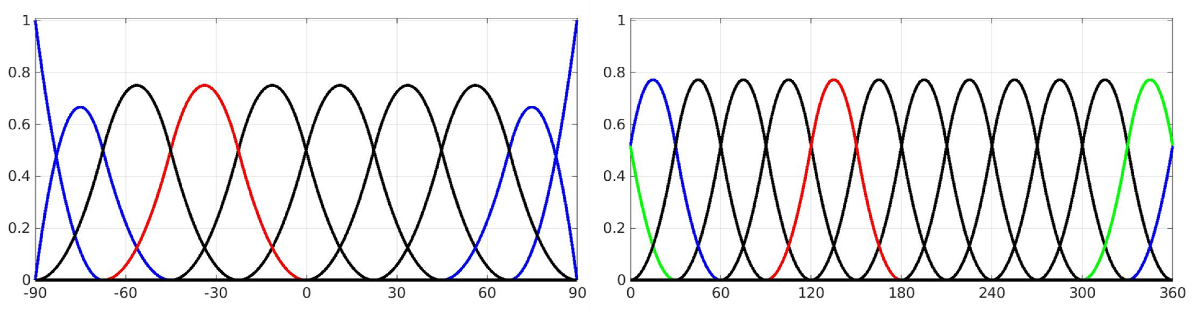
of levels and with respect to and . The tensor product (11) consists of so-called endpoint interpolating polynomial B-spline functions , which are used for the representation of the latitudinal dependencies. The trigonometric B-splines in longitude direction ensure a continuous representation of VTEC along the circles of latitudes [29]. The B-spline levels and define the total number and of B-spline functions and and the shift parameters and are their position along the latitude and the longitude. Figure 1 shows the polynomial B-spline functions of level (left) where the first and the last two splines indicate the endpoint interpolating feature. The right panel in Figure 1 shows the trigonometric B-splines of level with two splines crossing the 360° meridian. This feature allows for a continuous representation around the globe; more information can be found in [15,22,23,29].
In contrast to SHs, B-splines are localizing basis functions, i.e., they are different from zero only in small intervals, see the red colored B-spline functions in Figure 1. This means that for the estimation of unknown series coefficients, each tensor product (11) must be supported by observations to avoid singularities, [14,15,16,17]. In this regard, the B-spline levels and have to be chosen carefully. Similar to the calculation of the maximum degree (9), the levels depend on the mean sampling intervals and and the inequalities
have to be fulfilled, see [15,22,23]. Note, the higher the levels are chosen, the more spline functions are distributed along the latitude and the longitude and the finer are the structures in terms of wavelengths in latitude and in longitude that can be represented [15,16].
2.4. VTEC Products
Given the vector of estimated series coefficients for a time moment , the estimated values at arbitrary points with latitudes and longitudes , with , can be calculated by
Therein, is the vector of the values , the matrix comprises the underlying basis functions as shown in Equation (4).
Consequently, two strategies for disseminating ionospheric corrections can be set up. For each one, an appropriate product type is defined, which provides the information about the state of the ionosphere, namely
- Product type 1: estimated series coefficients with . It is assumed that a user has an appropriate converter for evaluating the respective series expansion (4). In that way, the corrections can directly be calculated by the user.
- Product type 2: VTEC grid values for latitudes and longitudes , where L is the number of points along the meridians and R is the number of grid points along the circles of latitudes with arbitrary sampling and , respectively. This implies that a user has to interpolate between the provided grid points in order to obtain the required correction.
In the following, we distinguish between grid-based Product type 2 formats (Section 2.5.1) and coefficient-based Product type 1 formats (Section 2.5.2).
2.5. Dissemination Formats for Positioning
To improve positioning by GNSS, ionospheric effects on the signals have to be corrected. Ionospheric corrections are therefore typically provided in terms of VTEC maps. The type of application (real-time, post-processing) determines the Product type to be used. For a proper application of the corrections, the preliminary position of the receiver and the position of the GNSS satellites are required. These allow the determination of the position vector of the IPP and subsequently the determination of the ionospheric correction either from Product type 1 or from Product type 2.
2.5.1. IONEX Format
The IONEX format was introduced by Schaer et al. in 1998 [6] and is up to now commonly used for the dissemination of GIMs of any type of latency. The format is particularly advantageous, because it allows for provision of additional information such as used receiver stations as well as DCBs. Usually, the VTEC values are given in an Earth-fixed geographic coordinate system on grids with a spatial sampling of ° in latitude and in longitude for snapshot maps with a temporal sampling of h.
When providing corrections using grid-based formats, the user must first perform an interpolation between the grid points and the temporal snapshot maps [6,15]. In order to calculate the values for the position of the IPPs with and for time , the simple bilinear spatial interpolation from VTEC values of the surrounding four points, as well as the temporal interpolation for any arbitrary time with according to Schaer et al. (1998) [6] can be applied. By applying the interpolation, the quality of the calculated VTEC values depends on the position of within the grid cell, on the spatial sampling intervals and , as well as the temporal sampling . The interpolation is applied in Sun-fixed coordinate system in order to take into account the Earth’s rotation, see [6].
2.5.2. Coefficient Based Format
The currently preferred method for dissemination of ionospheric corrections for RT positioning is based on SH coefficients, follows Product type 1 and is based on RTCM streams. The SSR VTEC message allows the dissemination of estimated coefficients of a SH model with additional information about degree n and order m of the underlying SH model, as well as the time moments and the height H of the single layer model for which the coefficients are valid. According to the message specifications the coefficients must be provided in Sun-fixed longitude with a phase shift of 2 h to the approximate VTEC maximum at 14:00 local time. This means that a coordinate transformation must be carried out for the values , which first provides a transformation from GSM to the Sun-fixed geographic coordinate system and then a rotation around the spin-axis of the Earth by 2 h. The SSR VTEC message is designed for the dissemination of SH coefficients and allows them only up to degree and order . This means that higher resolution models cannot be distributed via the SSR VTEC message. Another restriction of the message is that models not based on SHs require always a transformation to SHs.
2.5.3. Requirements for GIM Formats
The strategy for the dissemination and thus the choice of Product type 1 or Product type 2 of the estimated VTEC information is subject to certain restrictions, depending on their further use, namely:
- …
- For precise positioning in post processing mode: to be more specific, as long as the data are not immediately used by a user, the size of the data is less important and the transformation may take longer. Which means, the VTEC information can be prepared with high resolution and quality and be provided to the user. It does not matter which dissemination strategy is chosen and through which platform (FTP, streaming) the information reaches the user.
- …
- For precise navigation and positioning in RT: in this case, the selection of possible dissemination formats is limited. Hence, the user must receive the ionospheric information within seconds and with high precision, in order to correct the GNSS measurements used for positioning. Currently, only the SSR VTEC message is used for this purpose. Consequently, the dissemination strategy with Product type 1 has to be chosen.
3. Methodology
For the dissemination of a B-spline-based RT ionospheric correction to a user by means of Product type 1 and the currently intended data format, i.e., the SSR VTEC message, a transformation of the B-spline model into SH coefficients is required. For the transformation of the B-spline model, it must be considered that:
- The transformation should be done with high precision, i.e., since B-splines and SHs are characterized by different features, a high degree of the SH expansion needs to be considered.
- The time which is needed for the transformation is limited. Hence, the processing time including the generation of pseudo-observations—the evaluation of Equation (18)—and the estimation of the SH coefficients (cf. Equation (20)) should be completed within seconds.
3.1. Point Distribution on a Sphere
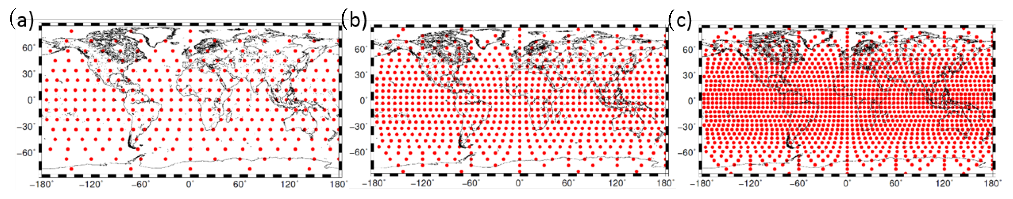
The transformation of the B-spline model to SHs requires input data generated by the B-spline model which reflect the variations in the GIM globally, i.e., VTEC values given as pseudo-observations on a global grid. As a matter of fact, a reliable computation of SH series coefficients requires homogeneously distributed input data. Since a regular grid as described in Section 2.5 does not fulfill this criterion, a Reuter grid is used instead [26]. The Reuter grid provides equi-distributed points on the sphere with spherical coordinates
for and with and the sampling intervals in latitude direction. Furthermore,
means the total number of grid points along the circle of latitude . Reforming of Equation (17) results in the sampling interval of the grid points in longitude direction. For , it applies . More information about the Reuter grid can be found in [27,30].
The left part of the Table 2 shows for different values of the values of the spatial sampling intervals along the meridian and at the equator, as well as the total number V of Reuter grid points. The right part of Table 2 provides, for each degree , the necessary mean sampling intervals and from Equation (9) and the corresponding total number of coefficients N.
The Reuter grid is particularly advantageous for the RT conversion of the B-spline model to SHs, because it provides a homogeneous distribution of the pseudo-observations and fulfills at the same time the conditions of the inequalities (9). Furthermore, a small number V of pseudo observations allows a transformation with short processing time. The values and for Reuter grids of in the left part of Table 2 fulfill the conditions (9) for SHs with maximum degrees in the right part.
Figure 2 shows the distribution of Reuter grid points with different values for . Due to the projection in the map, the Reuter grid points diverge with increasing latitude.
3.2. Pseudo Observations from B-spline Model Output
The pseudo observations are generated by means of the given vector of estimated B-spline coefficient of levels and with for the time moment . We rewrite Equation (13) for the B-spline case as
with the design matrix consisting B-spline tensor products according Equation (11). is a vector comprising the values , with the index R indicating the VTEC values on a Reuter grid.
3.3. Estimation of SH Coefficients from Reuter Grid
The series coefficients are estimated by parameter estimation from pseudo observations . By rewriting the observation Equation (7), the linear equation system
can be established, with the consistency vector , the vector of series coefficients, as well as the design matrix comprising the functions according to (8). In case of a matrix with full column rank, the problem can be solved by
Substituting Equation (18) for the observations vector the transformation between the B-spline and the SH coefficients is established and reads
with the transformation matrix .
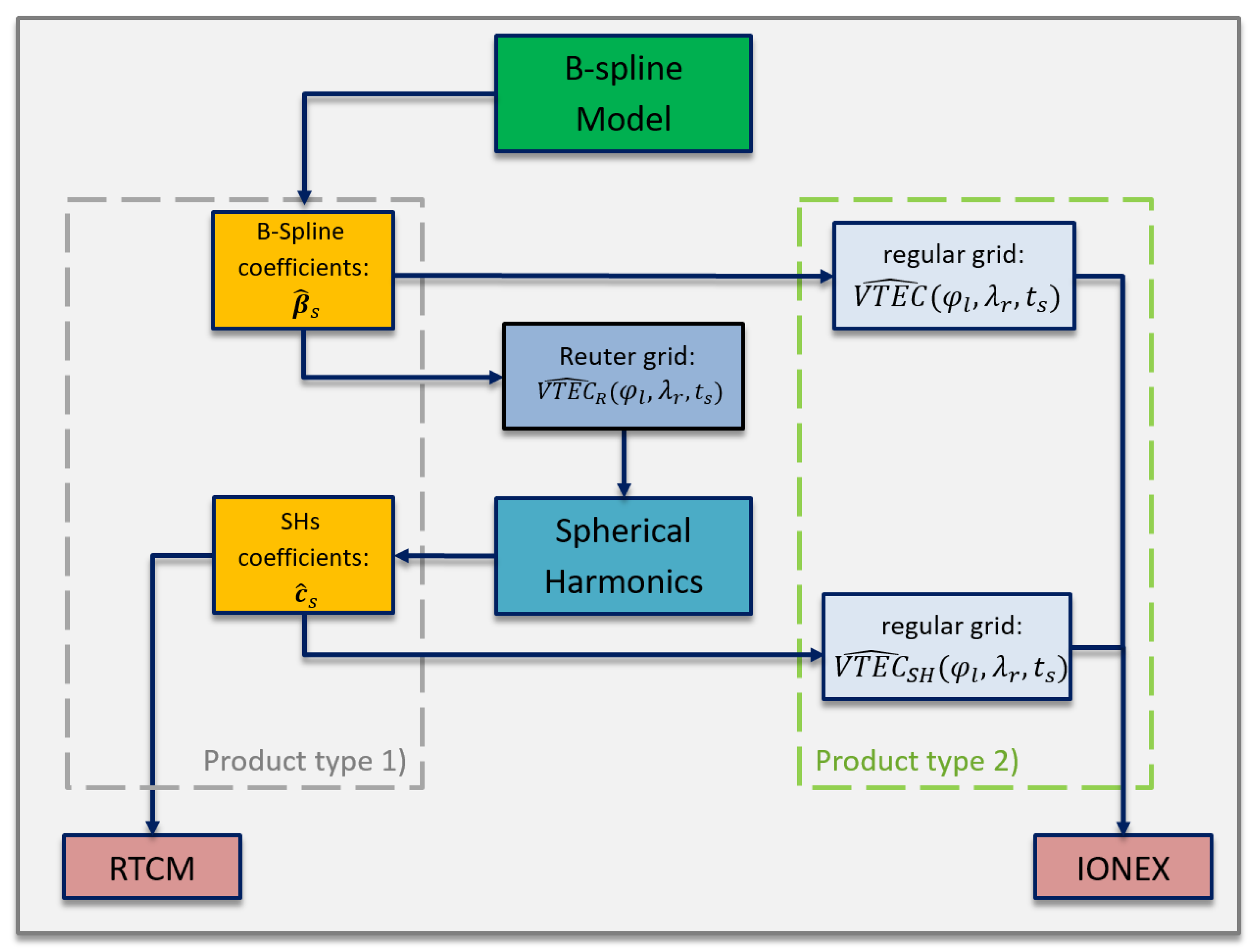
With the estimated coefficients , the Product type 1 and Product type 2 can be distributed to users (cf. Section 2.4). Figure 3 shows a flowchart on the methodology of the previously derived transformation method. Thereby the generation of pseudo-observations on a Reuter grid by means of given B-spline coefficients is followed by the estimation of the SH coefficients. The different sets and of coefficients can be considered for the dissemination in terms of Product type 1, however, only the set can be disseminated by means of the SSR VTEC message. Furthermore, both sets allow the generation of Product type 2. The two versions generated by B-splines and generated by means of the transformation method are depicted on the right hand side of the flowchart in Figure 3. Both grids can be disseminated by means of the IONEX file format.
4. Results and Discussion
Subsequently, the developed approach will be applied for the period from 2 September 2017 to 12 September 2017. This period was chosen because of the varying ionospheric activity. Hence, the period is in the decreasing phase of the last solar cycle with a moderate number of sunspots. In addition, solar flares occurred between September 4 to September 8 with the consequence of a geomagnetic storm and increased values for the Kp index up to the value 8.
Given are the B-spline coefficients in the Sun-fixed coordinate system of the B-spline series expansion with the levels and for the mentioned period. At this stage, it should be mentioned that the present B-spline model according to Goss et al. [15] and Erdogan et al. [17] was generated by means of hourly GNSS observations and ultra-rapid GNSS orbits and that it is classified as an ultra-rapid GIM according to the definition from the introduction.
According to [15] and to Table 3, an expansion in terms of polynomial B-splines with the level can be identified by a cutoff frequency of in SHs. An expansion in terms of trigonometric B-splines with the level corresponds to a cutoff frequency . The ionosphere usually shows structures that follow the geomagnetic equator and thus, stronger variations occur in latitude direction. Therefore, a higher spectral resolution is chosen in the latitude direction and a lower spectral resolution in the longitude direction. Since the spectral representation in latitude and longitude directions are very different for the given B-spline model, different cases are considered in the following to test and validate the determined approach.
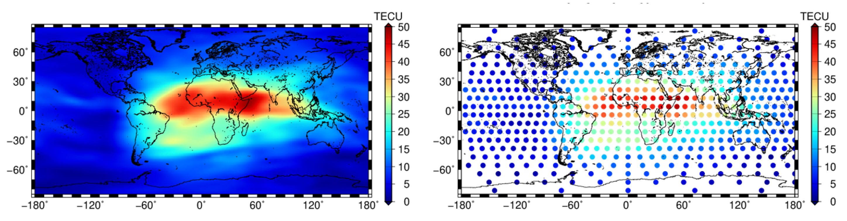
Following Section 3.1 and Section 3.2, we generate the pseudo-observations on Reuter grids for different values of . Figure 4 shows an example for September 8, at 12:00 UT with the VTEC map and modeled with B-splines in the left column. The right column depicts the pseudo-observation on the Reuter grid with .
Thereafter, five different transformation cases are considered and the SH coefficients are estimated by the parameter estimation as described in Section 3.3. Thereby, the requirements for the transformation, which were defined in the beginning of Section 3 were taken into account. The values for , as well as for the highest degree of the SH series expansion were used according to Section 3.1 and Table 2. Table 4 presents the five cases, which are analyzed in the following for their quality and feasibility. For quality estimation we follow the flowchart shown in Figure 3 and generate both the original B-spline GIM for and the transformed version on a regular grid. The quality characteristics, RMS (%, TECU), mean value , maximum value and minimum value are determined based on the deviations, i.e., the differences between the original GIM and the SH GIM. The applicability of the approach is executed on the basis of the necessary processing time per epoch, which is needed for the transformation. For comparison reasons, the transformations have been computed on a workstation with 64 GB RAM, and a 8 core processor of 3.2 GHz clock rate. Thereby comprises the evaluation time for the pseudo-observations as well as the estimation of the SH coefficients. All values given in Table 4 are averages obtained from transformed version computed with a min temporal sampling within the designated time span.
In the following, we discuss the given cases in more detail. In the first case, with pseudo-observations given on a Reuter grid with , an SH series expansion with degree and coefficients has to be estimated. The average processing time for the transformation took s. However, the transformed version with degree produces systematic errors compared to the original GIM. The RMS value of the deviations shows with 1.31 TECU significant differences. The relative RMS value
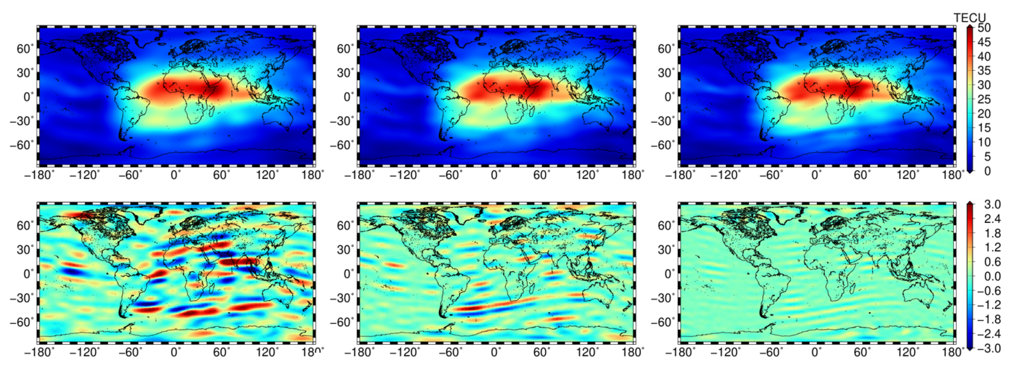
provides the RMS in percentage with 9.23% for the first case. The first column in Figure 5 shows the SH GIM in the top panel and the deviation map in the bottom panel. The deviation map represents mainly stripes in east–west direction, which indicate the difference in the spectral resolution for latitude direction between the original GIM corresponding to and representing the minimum wavelengths of ° and the SH GIM of , representing minimum of wavelengths (cf. Table 3). Visible are deviations with maximum values of TECU and minimum TECU, whereas the average is close to 0 TECU. In the second case, both the grid resolution and the degree of the SH expansion are increased to and , respectively. This causes an insignificant increase in computation time to s, but a significant improvement in the transformation accuracy to a relative RMS of 5.83% (cf. Table 4). For the third case, the processing time doubles compared to the first case with s, but the error of the transformation is reduced by a half and a relative RMS of 4.19% can be achieved. This improvement is also visible in the second column of Figure 5. Due to the increased degree of the SHs, finer structures in latitude direction can be represented better than in the first case. Therefore, the stripes in east–west direction in the deviation map show a smaller extension in latitude direction and occur with decreased magnitude of TECU and TECU.
Further improvements can be achieved by increasing the degree of the SH expansion for the transformation, but with a further extension of the processing time per epoch. The transformation using needs an average transformation time of s per epoch. The corresponding SH GIM is shown in the top right panel in Figure 5. The east–west stripes in the deviation map below are mainly visible in the area of the equatorial anomaly with maximum values of TECU and minimum values of TECU. The SH GIM describes a relative RMS of 1.83% compared to the original GIM. For these five cases, it can be concluded that the quality of the transformation improves with increasing degree for the SH series expansion.
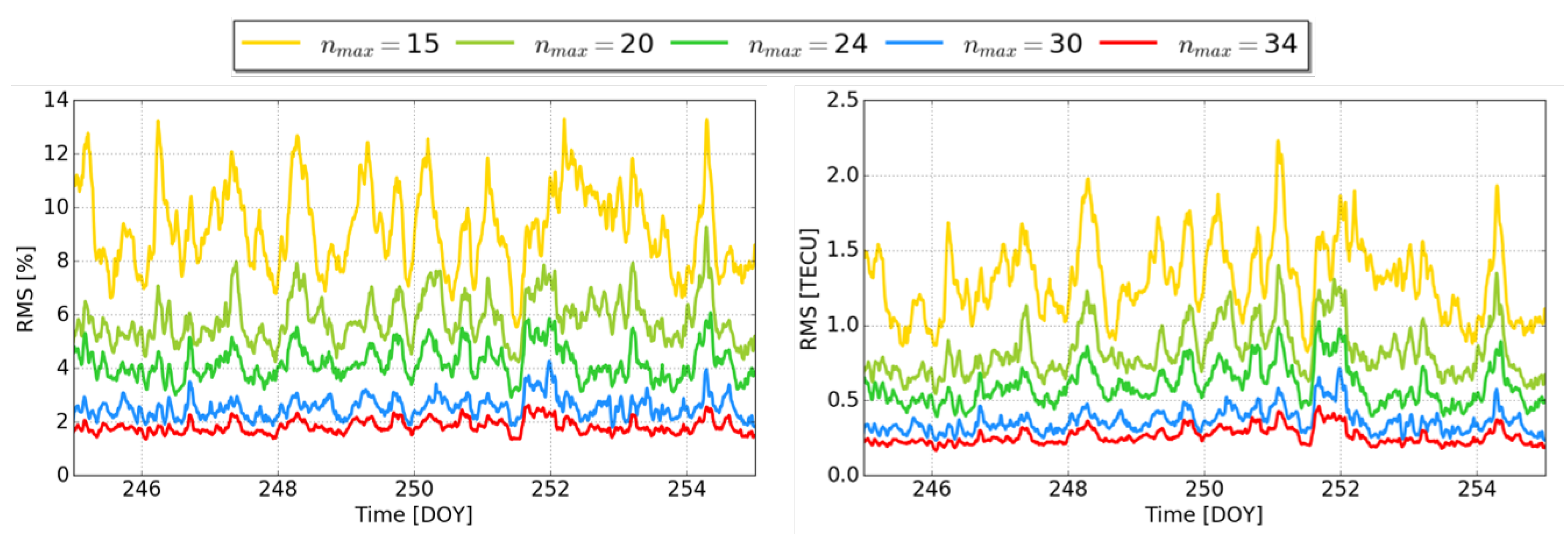
Accordingly, Figure 6 shows on the left the relative RMS values and on the right the RMS values of the deviations for the period from 2 September 2017 and 12 September 2017 with decreasing magnitude.
4.1. Validation
Subsequently, the original B-spline GIM and its transformed versions are validated using the dSTEC analysis and tested for their ability to correct the ionospheric disturbances in single frequency positioning. Additionally, the GIMs of the IAACs CODE from Berne, Switzerland and UPC from Barcelona, Spain are used for comparison.
4.1.1. dSTEC Analysis
The dSTEC analysis is one of the most commonly used validation method for GIMs. It is based on the comparison of differenced STEC observations of a receiver and satellite pair along its phase-continuous arc, with the differenced STEC values computed from the GIM to be validated as
with expectation value . Note, the STEC values from the GIMs are obtained by applying the mapping from Equation (3) and by the applying the interpolations from Section 2.5.1 according to Schaer et al. (1998) [6] for the position and time of the IPP of the observations along the satellite arc. More detailed information on the dSTEC analysis can be found in [15,18,24].
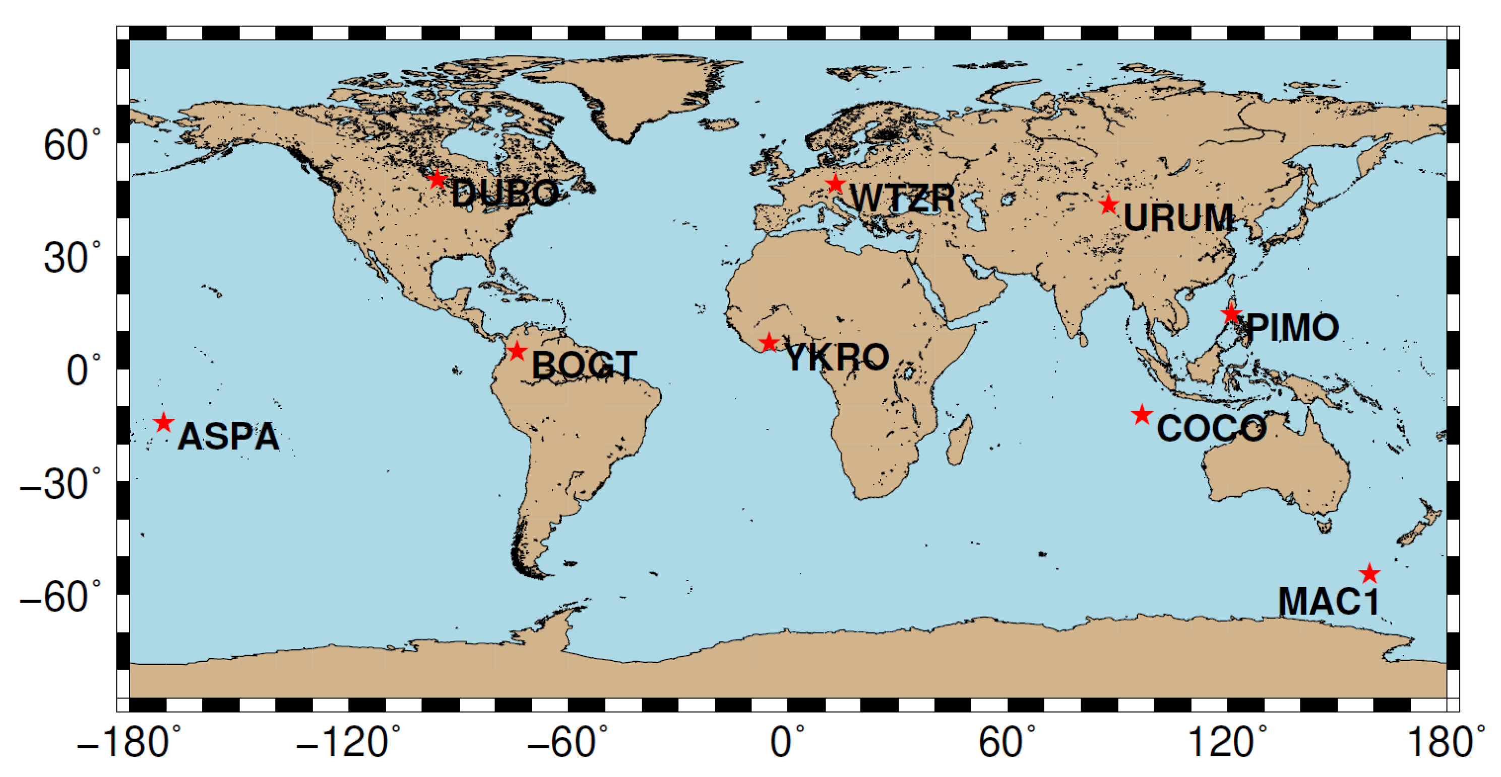
For the calculation of , the receiver stations shown in Figure 7 are used. These are either independent of the GIMs to be validated or have contributed to all of their calculations. Table 5 provides a summary of the results of the dSTEC analysis. The original B-spline GIM of DGFI-TUM is called ‘othg’. The naming follows the definition in [15], where ‘o’ stands for the OPTIMAP processing software, which was developed in a third-party project (see Acknowledgments). The second digit describes the temporal output sampling with ‘t’ for ten minutes. The ’h’ describes the high spectral resolution and the ‘g’ the global expansion. The transformed versions of the ‘othg’, coinciding with the different cases of the previous section are named accordingly, but with the respective degree of SHs used for the transformation in the second and third digit. The last two columns in Table 5 show the results for the GIMs ‘codg’ and ‘uqrg’ provided by CODE and UPC, respectively. All GIMs used in the dSTEC analysis are given in IONEX format with spatial sampling of ° in latitude and in longitude. All other specifications for the different GIMs are depicted in Table 5.
The last row shows the RMS values of , Equation (23), for each GIM given as the average over all stations and all observations during the period in September 2017. They indicate the performance of the individual GIMs during the designated period and for the selected stations. As usual the ‘uqrg’ performs best in the selection of GIMs with an RMS of 0.85 TECU, followed by ‘othg’ with an RMS of 0.91 TECU. The transformed versions show a trend that was already shown in Figure 6; the RMS values of transformed versions with larger approach the value of the original ‘othg’. With an RMS of 0.92 TECU, the ‘o34g’ has a negligible difference in the accuracy to ‘othg’. This confirms their approximate agreement in the spectral resolution with for ‘o34g’ and the cutoff frequency of (cf. Table 3) in the latitude direction of ‘othg’. A comparison of the GIMs ‘o15g’ and ‘codg’, both based on an SH series expansion of , shows that a higher degree for the transformation is necessary, since the original GIM ‘othg’ provides a higher and ‘o15g’ a less quality than the ‘codg’ during the period of investigation.
4.1.2. GIM Performance in Single-Frequency PPP
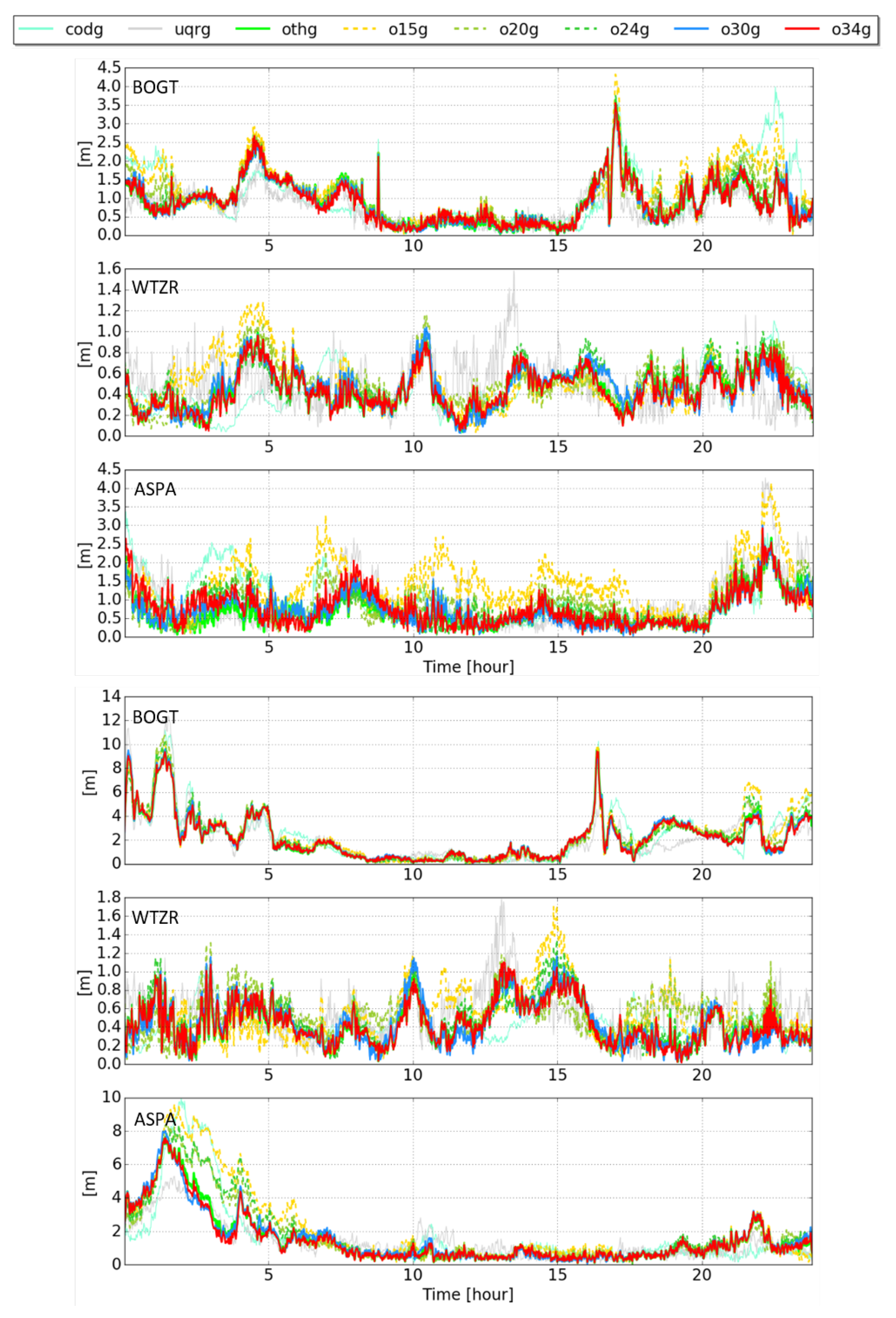
We perform a Precise Point Positioning (PPP) for the stations BOGT, WTZR and APSA using the open source software RTKLIB [25,32]. The selection of stations covers both mid and low latitudes, see Figure 7, as well as regions with different characteristics for ionospheric modeling, i.e., either characterized with strong variations in VTEC (BOGT), dense observation distribution (WTZR) or low number of observations (ASPA). A kinematic processing mode is selected for each station to estimate the position for each epoch for which an observation was available. The VTEC values provided in the GIM are used to correct the ionospheric delay for each single frequency observation of the stations. Positioning tests were performed for the days 2 September 2017 with moderate ionospheric activity and 8 September 2017 characterized by a geomagnetic storm.
The estimated coordinate components , and are subtracted from the actual coordinates , and provided by the IGS [33] and the deviations of the 3D position are determined as
Figure 8 shows the time series of the differences for 2 September 2017 (left) and 8 September 2017 (right). A significant difference can be seen in between the two days. On 8 September 2017, due to the high geomagnetic activity the ionospheric corrections are more difficult to determine and thus, the positioning accuracy decreases and the deviations increase. This trend is especially noticeable for the stations BOGT and APSA close to the equator. It can also be observed that their deviations increase during local noon, i.e., between 15:00 and 20:00 UT for BOGT and between 20:00 and 24:00 UT for ASPA. The large deviations of the position of BOGT and ASPA between 00:00 and 05:00 UT on September 8 are due to the high geomagnetic variations with increased geomagnetic index of . The variations are not as significant at the station WTZR, which was located on the night side of the Earth at that time. The daily variations of S in Figure 8 show that ‘othg’, ‘o30g’ and ‘o34g’, in light green, blue and red, respectively, exhibit a similar variation. Stronger deviations and mostly larger values can be recognized for the GIMs ‘o15g’, ‘o20g’ and ‘o24g’ with the dashed lines. The GIM ‘codg’ shows a similar behavior during the days. However, the ’uqrg’ performs better in single frequency positioning and sometimes shows lower values than the ‘othg’, the ’o30g’ and the ‘o34g’, except at local noon at station WTZR, where it shows large deviations.
A detailed evaluation of the performance of the different GIMs is performed using the respective RMS and the average values of the time series , which are depicted in Table 6.
The color scheme in Table 6 implies the lowest and highest values of the RMS and in green and red, for the respective station and day. It can be seen that for all stations there are differences in the positioning accuracy between the two days examined. Hence, for DOY 251, the RMS and average values are increased. There is an additional trend which shows, that for the selected stations and days the high resolution GIMs, ‘othg’ and ‘uqrg’ allow a correction of the ionospheric disturbances in a way that leads to a positioning with increased accuracy (see the green colors). Furthermore, the poor performance of the ‘o15g’—which has mostly highlighted values in red—confirms the result from Section 4.1.1, that a transformed version a with higher degree of SH series expansion is necessary to achieve the quality of the original GIM. As the degree of SHs for the transformation increases, the accuracy of positioning increases when using their ionosphere corrections. The values written in bold in Table 6 allow the conclusion that a transformation with at least the maximum degree is necessary to achieve the quality of ’othg’.
It should be pointed out, that the pure SH model, the ’codg’, can correct the ionospheric disturbances for single frequency positioning better than the transformed version ‘o15g’. However, in the example shown here, ‘codg’ cannot achieve accuracy of the ‘othg’, the ’uqrg’ and the transformed versions ‘o30g’ and ’o34g’.
5. Summary and Conclusions
The dissemination of RT ionosphere information is currently based on the RTCM message 1264, which can provide SH coefficients up to a maximum degree of . The IGS started to provide a combined RT-GIM, collecting the GIMs from CAS, CNES and UPC using Ntrip protocol and the SSR VTEC message [21]. Since the SSR VTEC message is currently the only format type for dissemination the RT-GIMs of the IAACs, only SH models can be considered. Other models which are not based on SHs need to be converted and suffer from degeneration in the accuracy of the GIMs. Especially, high-resolution models cannot be converted appropriately to SHs when a low degree is used in the transformation. This means that an adaptation or extension of the existing dissemination formats, as already objected by Goss et al. (2019) and (2020) [15,16], must be carried out.
This paper presents a novel approach on the transformation of GIMs modeled by means of a B-spline series expansion to SH coefficients. It should be noted that the developed method can also be applied to models based on voxels or alternative basis functions.
The developed approach is setup in a way that the processing time during transformations are acceptable for RT applications and the transformed SH GIMs maintain the quality of the original GIM.
However, the numerical investigations are based on ultra-rapid GIMs modeled by a B-spline series expansion according to [15]. The given ultra-rapid GIMs only serve to test the developed approach and to assess the accuracy and quality of the transformations and the latency can further be decreased. The investigation period covers the days 2 September to 12 September 2017 with a geomagnetic storm on September 8. In a first step, a case study considering five cases with different degrees for the transformation to SH is shown. It was found that with an increased value , the transformations converge sufficiently with the original B-spline model. However, for a transformation of the given B-spline model with level values of and a degree of is required.
In the assessment comprising a dSTEC analysis and a single-frequency PPP, the models of CODE (SHs of —’codg’) and UPC (voxel and Kriging model—’uqrg’) were used for comparison with the B-spline GIM ‘othg’ and its transformed versions. For both assessment methods, the high-resolution GIMs ‘othg’ and ‘uqrg’ as well as the transformed versions with degrees performed the best. The single-frequency PPP shows a discrepancy between the transformed SH GIMs of lower degree and the original GIM ‘othg’, but also between ‘codg’ and the high-resolution solutions ‘othg’ and ’uqrg’.
Finally, it can be concluded that for a transformation of the B-spline model to SHs, the maximum degree has to be adapted accordingly. In this way, high quality ionospheric corrections can be provided to single-frequency users for the correction of positioning and navigation. This means that for the dissemination of high-resolution GIMs, an extension of the limited degree of the SH coefficients which is allowed by SSR VTEC message is required and accomplished urgently.
Author Contributions
The concept of the paper was proposed by A.G. and discussed with M.H.-P. and M.S., A.G. compiled the figures and wrote the text. The paper was reviewed by M.H.-P., M.S., D.R.-D., E.E., F.S., M.S. and F.S. assume responsibility for the projects INSIGHT II and OPTIMAP for which significant contributions entered into this article. The paper and figures were reviewed by all authors. All authors have read and agreed to the published version of the manuscript.
Funding
This research was funded by the German Research Foundation (DFG) under grant number SCHM2433/10-2 (project INSIGHT II) and the Technical University of Munich (TUM) in the framework of the Open Access Publishing Program. The approach presented in this paper was to a large part developed in the framework of the project OPTIMAP (‘Operational Tool for Ionospheric Mapping and Prediction’) funded by the Bundeswehr GeoInformation Center (BGIC) and the German Space Situational Awareness Centre (GSSAC).
Data Availability Statement
The data presented in this study are openly available in ftp://cddis.gsfc.nasa.gov/.
Acknowledgments
The authors thank the IGS and its IAACs, in particular the Center for Orbit Determination in Europe (CODE, Berne, Switzerland) and the Universitat Politècnica de Catalunya/IonSAT (UPC, Barcelona, Spain), for providing the data. We acknowledge the Generic Mapping Tool (GMT), which was primarily used for generating the figures in this work.
Conflicts of Interest
The authors declare no conflict of interest.
References
- Klobuchar, J.A. Ionospheric Time-Delay Algorithm for Single-Frequency GPS Users. IEEE Trans. Aerospace Electron. Syst. 1987, AES-23, 325–331. [Google Scholar] [CrossRef]
- Petit, G.; Luzum, B. IERS Conventions. Technical Report. 2010. Available online: www.iers.org (accessed on 21 December 2020).
- Hernández-Pajares, M.; Juan, J.M.; Sanz, J.; Argón-Àngel, A.; Garcia-Rigo, A.; Salazar, D.; Escudero, M. The ionosphere: Effects, GPS modeling and benefits for space geodetic techniques. J. Geod. 2011, 85, 887–907. [Google Scholar] [CrossRef]
- Langley, R.B. Propagation of the GPS Signals. In GPS for Geodesy; Teunissen, P.J.G., Kleusberg, A., Eds.; Springer: Berlin/Heidelberg, Germany, 1998; pp. 111–149. [Google Scholar] [CrossRef]
- Ciraolo, L.; Azpilicueta, F.; Brunini, C.; Meza, A.; Radicella, S. Calibration errors on experimental slant total electron content (TEC) determined with GNSS. J. Geod. 2007, 81, 111–120. [Google Scholar] [CrossRef]
- Schaer, S.; Gurtner, W.; Feltens, J. IONEX: The IONosphere Map EXchange Format Version 1; Technical Report; Astronomical Institute, University of Berne: Bern, Switzerland, 1998. [Google Scholar]
- The International GPS Service (IGS): An interdisciplinary service in support of Earth sciences. Adv. Space Res. 1999, 23, 631–653. [CrossRef]
- Feltens, J.; Schaer, S. IGS Products for the Ionosphere; Technical report; European Space Operation Centre and Astronomical Institue of the University of Berne: Bern, Switzerland, 1998. [Google Scholar]
- Villiger, A. (Ed.) International GNSS Service Technical Report 2018; Technical report, IGS Central Bureau and University of Bern; Bern Open Publishing: Bern, Switzerland, 2018. [Google Scholar]
- Li, Z.; Yuan, Y.; Wang, N.; Hernández-Pajares, M.; Huo, X. SHPTS: Towards a new method for generating precise global ionospheric TEC map based on spherical harmonic and generalized trigonometric series functions. J. Geod. 2015, 89, 331–345. [Google Scholar] [CrossRef]
- Hernández-Pajares, M.; Juan, J.M.; Sanz, J. New approaches in global ionospheric determination using ground GPS data. J. Atmos. Sol. Terr. Phys. 1999, 61, 1237–1247. [Google Scholar] [CrossRef]
- Hernández-Pajares, M.; Juan, J.M.; Sanz, J.; Orus, R.; Garcia-Rigo, A.; Feltens, J.; Komjathy, A.; Schaer, S.C.; Krankowski, A. The IGS VTEC map: A reliable source of ionospheric information since 1998. J. Geod. 2009, 83, 263–275. [Google Scholar] [CrossRef]
- Orus, R.; Hernández-Pajares, M.; Juan, J.; Sanz, J. Improvement of global ionospheric VTEC maps by using kriging interpolation technique. J. Atmos. Sol.-Terr. Phys. 2005, 67, 1598–1609. [Google Scholar] [CrossRef]
- Erdogan, E.; Schmidt, M.; Seitz, F.; Durmaz, M. Near real-time estimation of ionosphere vertical total electron content from GNSS satellites using B-spline in a Kalman Filter. Ann. Geophys. 2017, 35, 263–277. [Google Scholar] [CrossRef]
- Goss, A.; Schmidt, M.; Erdogan, E.; Görres, B.; Seitz, F. High-resolution vertical total electron content maps based on multi-scale B-spline representations. Ann. Geophys. 2019, 37, 699–717. [Google Scholar] [CrossRef] [Green Version]
- Goss, A.; Schmidt, M.; Erdogan, E.; Seitz, F. Global and Regional High-Resolution VTEC Modelling Using a Two-Step B-Spline Approach. Remote Sens. 2020, 12, 1198. [Google Scholar] [CrossRef] [Green Version]
- Erdogan, E.; Schmidt, M.; Goss, A.; Görres, B.; Seitz, F. Adaptive Modeling of the Global Ionosphere Vertical Total Electron Content. Remote Sens. 2020, 12, 1822. [Google Scholar] [CrossRef]
- Hernández-Pajares, M.; Roma-Dollase, D.; Krankowski, A.; García-Rigo, A.; Orús-Pérez, R. Methodology and consistency of slant and vertical assessments for ionospheric electron content models. J. Geod. 2017, 19, 1405–1414. [Google Scholar] [CrossRef]
- Caissy, M.; Agrotis, L.; Weber, G.; Pajares, M.; Hugentobler, U. The international GNSS real-time service. GPS World 2012, 23, 52–58. [Google Scholar]
- RTCM. IGS State Space Representation (SSR). Technical Report. 2020. Available online: https://files.igs.org/pub/data/format/igs_ssr_v1.pdf (accessed on 21 December 2020).
- Li, Z.; Wang, N.; Hernández-Pajares, M.; Yuan, Y.; Krankowski, A.; Liu, A.; Zha, J.; García-Rigo, A.; Roma, D.; Yang, H.; et al. IGS real-time service for global ionospheric total electron content modeling. J. Geod. 2020, 94, 1–16. [Google Scholar] [CrossRef]
- Schmidt, M.; Dettmering, D.; Mößmer, M.; Wang, Y. Comparison of spherical harmonic and B-spline models for the vertical total electron content. Radio Sci. 2011, 46, RS0D11. [Google Scholar] [CrossRef]
- Schmidt, M.; Dettmering, D. Using B-spline expansions for ionosphere modeling. In Handbook of Geomathematics, 2nd ed.; Freeden, W., Nashed, M.Z., Sonar, T., Eds.; Springer: Berlin/Heidelberg, Germany, 2015; pp. 939–983. [Google Scholar] [CrossRef]
- Roma-Dollase, D.; Hernández-Pajares, M.; Krankowski, A.; Kotulak, K.; Ghoddousi-Fard, R.; Yuan, Y.; Li, Z.; Zhang, H.; Shi, C.; Wang, C. Consistency of seven different GNSS global ionospheric mapping techniques during one solar cycle. J. Geod. 2017, 92, 691–706. [Google Scholar] [CrossRef] [Green Version]
- Takasu, T.; Yasuda, A. Development of the low-cost RTK-GPS receiver with an open source program package RTKLIB. In International Symposium on GPS/GNSS; International Convention Center: Jeju, Korea, 2009. [Google Scholar]
- Reuter, R. Über Integralformeln der Einheitsphäre und Harmonische SPlinefunctionen. Ph.D. Thesis, RWTH Aachen, Aachen, Germany, 1982. [Google Scholar]
- Freeden, W.; Grevens, T.; Schreiner, M. Constructive Approximation on the Sphere; Oxford University Press: Oxford, UK, 1998. [Google Scholar]
- Laundal, K.; Richmond, A. Magnetic Coordinate Systems. Space Sci. Rev. 2017, 206, 27–59. [Google Scholar] [CrossRef] [Green Version]
- Lyche, T.; Schumaker, L. A multiresolution tensor spline method for fitting functions on the sphere. SIAM J. Sci. Comput. 2001, 22, 724–746. [Google Scholar] [CrossRef] [Green Version]
- Eicker, A. Gravity Field Refinement by Radial Basis Functions from In-situ Satellite Data. Ph.D. Thesis, Rheinische Friedrich-Wilhelms-Universität Bonn, Bonn, Germany, 2008. [Google Scholar]
- Schaer, S. Mapping and Predicting the Earth’s Ionosphere Using the Global Positioning System. Ph.D. Thesis, University of Berne, Bonn, Germany, 1999. [Google Scholar]
- Prol, F.; Camargo, P.; Monico, J.; Muella, M. Assessment of a TEC calibration procedure by single-frequency PPP. GPS Solut. 2018, 22, 35. [Google Scholar] [CrossRef] [Green Version]
- Dow, J.; Neilan, R.E.; Rizos, C. The International GNSS Service in a changing landscape of Global Navigation Satellite Systems. J. Geod. 2009, 83. [Google Scholar] [CrossRef]
Figure 1.
Polynomial B-spline of level (left). The blue-colored splines indicate the endpoint interpolating feature at the boundaries of the interval. In the right panel, the trigonometric B-spline of level (right) are represented. Here, the blue-colored spline as well as the green-colored spline indicate the wrapping around at the boundaries of the 0° and 360° meridian. The red-colored B-spline functions are of shift parameters and for the polynomial and trigonometric B-splines, respectively.

Figure 2.
Reuter grids with values in panel (a), in panel (b) and in panel (c).

Figure 3.
Schematic representation of the transformation and the following generation of the products of type 1 and 2 and the typically used data formats SSR VTEC message and IONEX, respectively.
Figure 3.
Schematic representation of the transformation and the following generation of the products of type 1 and 2 and the typically used data formats SSR VTEC message and IONEX, respectively.

Figure 4.
Original global ionosphere map (GIM) generated by the B-spline model with levels and in the left column. In the right column are the pseudo observations on a Reuter grid with .
Figure 4.
Original global ionosphere map (GIM) generated by the B-spline model with levels and in the left column. In the right column are the pseudo observations on a Reuter grid with .

Figure 5.
SH GIM (top panels) and deviation maps (bottom panels) of the 1. (left column), 3. (middle column) and 5. (right column) test case from Table 4 for September 8, at 12:00 UT.
Figure 5.
SH GIM (top panels) and deviation maps (bottom panels) of the 1. (left column), 3. (middle column) and 5. (right column) test case from Table 4 for September 8, at 12:00 UT.

Figure 6.
Change in relative RMS values (left) and RMS values (right), for the period from 2 September 2017 (DOY 245) to 12 September 2017 (DOY 255); temporal sampling intervals of 10 min.
Figure 6.
Change in relative RMS values (left) and RMS values (right), for the period from 2 September 2017 (DOY 245) to 12 September 2017 (DOY 255); temporal sampling intervals of 10 min.

Figure 7.
Global distribution of 9 receiver stations that are used for the dSTEC validation and for comparison of the generated GIMs.
Figure 7.
Global distribution of 9 receiver stations that are used for the dSTEC validation and for comparison of the generated GIMs.

Figure 8.
Differences in the 3D position between the position determined by Precise Point Positioning (PPP) and ionospheric corrections calculated by different GIMs and the actual position. Left side shows the differences for the stations BOGT, WTZR and ASPA during the 2 September 2017 (DOY 245) and the right side the corresponding differences for 8 September 2017 (DOY 251) with different scaling of the y-axis. On the x-axis, the time in UT is depicted in hours.


Table 1.
Definition of different latency types depending on the input data.
| Latency Type | Final | Rapid | Ultra-Rapid | Near Real-Time | Real-Time |
|---|---|---|---|---|---|
| Data | post-processed | daily | hourly | data-streams | data-streams |
| Data Latency | 2–3 weeks | >1 day | >1 h | real-time | real-time |
| Product Latency | 2–3 weeks | >1 day | >1 h | <15 min | <1 min |
Table 2.
Sampling intervals and of the Reuter grid points for different values of and the corresponding number V of Reuter grid points. Required max. sampling intervals and and the number of unknown coefficients of spherical harmonics (SHs) with different values for .
Table 2.
Sampling intervals and of the Reuter grid points for different values of and the corresponding number V of Reuter grid points. Required max. sampling intervals and and the number of unknown coefficients of spherical harmonics (SHs) with different values for .
| Reuter Grid | Spherical Harmonics | ||||||||||
|---|---|---|---|---|---|---|---|---|---|---|---|
| 16 | 21 | 25 | 31 | 35 | 15 | 20 | 24 | 30 | 34 | ||
| , | 11.25° | 8.57° | 7.2° | 5.8° | 5.14° | , | 12 | 9 | 7.5 | 6 | 5.3 |
| V | 317 | 563 | 797 | 1225 | 1561 | N | 256 | 441 | 625 | 961 | 1224 |
Table 3.
Different values for B-spline levels and with their corresponding values for the cutoff frequency and the minimum wavelengths and (see Goss et al., 2019 and 2020 [15,16]).
| Polynomial B-Splines | Trigonometric B-Splines | ||||||||||||
|---|---|---|---|---|---|---|---|---|---|---|---|---|---|
| 1 | 2 | 3 | 4 | 5 | 6 | 1 | 2 | 3 | 4 | 5 | 6 | ||
| 3 | 5 | 9 | 17 | 33 | 63 | 3 | 6 | 12 | 24 | 48 | 96 | ||
| 120° | 72° | 40° | 21° | 10.9° | 5.7° | 120° | 60° | 30° | 15° | 7.5° | 3.75° | ||
Table 4.
Numerical and statistical results to estimate the quality and feasibility for the different cases.
Table 4.
Numerical and statistical results to estimate the quality and feasibility for the different cases.
| 1. Case | 2. Case | 3. Case | 4. Case | 5. Case | |
|---|---|---|---|---|---|
| 16 | 21 | 25 | 31 | 35 | |
| V | 317 | 563 | 797 | 1225 | 1561 |
| 15 | 20 | 24 | 30 | 34 | |
| N | 256 | 441 | 625 | 961 | 1224 |
| 1.43 s | 1.85 s | 3.12 s | 4.99 s | 8.23 s | |
| rel. RMS [%] | 9.23 | 5.83 | 4.19 | 2.54 | 1.83 |
| RMS [TECU] | 1.31 | 0.83 | 0.60 | 0.36 | 0.26 |
| [TECU] | 8.22 | 5.91 | 5.23 | 2.22 | 1.79 |
| [TECU] | −8.06 | −6.29 | −4.21 | −2.23 | −1.9 |
| [TECU] | 0.016 | 0.0012 | 0.014 | 0.0033 | 0.003 |
Table 5.
Comparison of GIMs with different characteristics, i.e., model type, degree of series expansion (, , ), temporal output sampling intervals () and latency until provision. For each of the investigated GIMs, the RMS of the dSTEC analysis is given.
Table 5.
Comparison of GIMs with different characteristics, i.e., model type, degree of series expansion (, , ), temporal output sampling intervals () and latency until provision. For each of the investigated GIMs, the RMS of the dSTEC analysis is given.
| GIM | othg | o15g | o20g | o24g | o30g | o34g | codg | uqrg |
|---|---|---|---|---|---|---|---|---|
| Model | B-Splines | SHs | SHs | SHs | SHs | SHs | SHs | Voxel & Kriging |
| 15 | 20 | 24 | 30 | 34 | 15 | n.a. | ||
| / | 5/3 | |||||||
| 10 min | 10 min | 10 min | 10 min | 10 min | 10 min | 60 min | 15 min | |
| Latency | <3 h | <3 h | <3 h | <3 h | <3 h | <3 h | >1 week | >1 day |
| Reference | [15] | Section 3 | Section 3 | Section 3 | Section 3 | Section 3 | [31] | [13] |
| RMS [TECU] | 0.91 | 1.18 | 1.05 | 1.00 | 0.93 | 0.92 | 1.01 | 0.85 |
Table 6.
RMS and values of deviations for September 2 (DOY 245) and 8 (DOY 251), 2017 at the stations BOGT, WTZR and ASPA. The maximum and minimum values of the RMS and are marked in red and green, respectively. The RMS and of the transformed versions are bold if they are lower than the values of the original GIM, ‘othg’.
| Value | DOY | othg | o15g | o20g | o24g | o30g | o34g | codg | uqrg | |
|---|---|---|---|---|---|---|---|---|---|---|
| BOGT | RMS [TECU] | 245 | 1.07 | 1.35 | 1.17 | 1.09 | 1.05 | 1.05 | 1.29 | 0.90 |
| 251 | 2.91 | 3.19 | 3.12 | 3.03 | 2.91 | 2.86 | 3.14 | 2.98 | ||
| [TECU] | 245 | 0.90 | 1.13 | 1.00 | 0.92 | 0.89 | 0.89 | 1.05 | 0.77 | |
| 251 | 2.22 | 2.44 | 2.34 | 2.31 | 2.23 | 2.20 | 2.35 | 2.18 | ||
| WTZR | RMS [TECU] | 245 | 0.49 | 0.55 | 0.53 | 0.52 | 0.50 | 0.48 | 0.51 | 0.55 |
| 251 | 0.49 | 0.90 | 0.57 | 0.54 | 0.50 | 0.49 | 0.51 | 0.62 | ||
| [TECU] | 245 | 0.45 | 0.50 | 0.49 | 0.48 | 0.46 | 0.44 | 0.46 | 0.50 | |
| 251 | 0.44 | 0.53 | 0.52 | 0.47 | 0.44 | 0.44 | 0.47 | 0.57 | ||
| ASPA | RMS [TECU] | 245 | 0.81 | 2.53 | 0.98 | 0.92 | 0.85 | 0.92 | 1.13 | 1.19 |
| 251 | 2.18 | 3.12 | 2.59 | 2.67 | 2.17 | 2.11 | 2.65 | 1.80 | ||
| [TECU] | 245 | 0.69 | 1.37 | 0.86 | 0.79 | 0.73 | 0.77 | 0.95 | 0.94 | |
| 251 | 1.53 | 2.10 | 1.76 | 1.84 | 1.54 | 1.48 | 1.64 | 1.40 |
Publisher’s Note: MDPI stays neutral with regard to jurisdictional claims in published maps and institutional affiliations. |
© 2020 by the authors. Licensee MDPI, Basel, Switzerland. This article is an open access article distributed under the terms and conditions of the Creative Commons Attribution (CC BY) license (http://creativecommons.org/licenses/by/4.0/).
Share and Cite
MDPI and ACS Style
Goss, A.; Hernández-Pajares, M.; Schmidt, M.; Roma-Dollase, D.; Erdogan, E.; Seitz, F. High-Resolution Ionosphere Corrections for Single-Frequency Positioning. Remote Sens. 2021, 13, 12. https://doi.org/10.3390/rs13010012
AMA Style
Goss A, Hernández-Pajares M, Schmidt M, Roma-Dollase D, Erdogan E, Seitz F. High-Resolution Ionosphere Corrections for Single-Frequency Positioning. Remote Sensing. 2021; 13(1):12. https://doi.org/10.3390/rs13010012
Chicago/Turabian StyleGoss, Andreas, Manuel Hernández-Pajares, Michael Schmidt, David Roma-Dollase, Eren Erdogan, and Florian Seitz. 2021. "High-Resolution Ionosphere Corrections for Single-Frequency Positioning" Remote Sensing 13, no. 1: 12. https://doi.org/10.3390/rs13010012
Note that from the first issue of 2016, this journal uses article numbers instead of page numbers. See further details here.