Article

Integrating Remote Sensing and Landscape Characteristics to Estimate Soil Salinity Using Machine Learning Methods: A Case Study from Southern Xinjiang, China

1
Institute of Agricultural Remote Sensing and Information Technology Application, College of Environmental and Resource Sciences, Zhejiang University, Hangzhou 310058, China
2
College of Plant Science, Tarim University, Alar 843300, China
3
School of Environmental Sciences, University of Guelph, Guelph, ON N1G2W1, Canada
4
College of Biosystems Engineering and Food Science, Zhejiang University, Hangzhou 310058, China
5
Key Laboratory of Spectroscopy Sensing, Ministry of Agriculture, Hangzhou 310058, China
*
Author to whom correspondence should be addressed.
Remote Sens. 2020, 12(24), 4118; https://doi.org/10.3390/rs12244118
Submission received: 13 November 2020 / Revised: 8 December 2020 / Accepted: 12 December 2020 / Published: 16 December 2020
(This article belongs to the Special Issue Advances of Proximal and Remote Sensing in Soil Salinity Mapping)

Abstract

:
Soil salinization, one of the most severe global land degradation problems, leads to the loss of arable land and declines in crop yields. Monitoring the distribution of salinized soil and degree of salinization is critical for management, remediation, and utilization of salinized soil; however, there is a lack of thorough assessment of various data sources including remote sensing and landscape characteristics for estimating soil salinity in arid and semi-arid areas. The overall goal of this study was to develop a framework for estimating soil salinity in diverse landscapes by fusing information from satellite images, landscape characteristics, and appropriate machine learning models. To explore the spatial distribution of soil salinity in southern Xinjiang, China, as a case study, we obtained 151 soil samples in a field campaign, which were analyzed in laboratory for soil electrical conductivity. A total of 35 indices including remote sensing classifiers (11), terrain attributes (3), vegetation spectral indices (8), and salinity spectral indices (13) were calculated or derived and correlated with soil salinity. Nine were used to model and estimate soil salinity using four predictive modelling approaches: partial least squares regression (PLSR), convolutional neural network (CNN), support vector machine (SVM) learning, and random forest (RF). Testing datasets were divided into vegetation-covered and bare soil samples and were used for accuracy assessment. The RF model was the best regression model in this study, with R2 = 0.75, and was most effective in revealing the spatial characteristics of salt distribution. Importance analysis and path modeling of independent variables indicated that environmental factors and soil salinity indices including digital elevation model (DEM), B10, and green atmospherically resistant vegetation index (GARI) showed the strongest contribution in soil salinity estimation. This showed a great promise in the measurement and monitoring of soil salinity in arid and semi-arid areas from the integration of remote sensing, landscape characteristics, and using machine learning model.

Graphical Abstract

1. Introduction

Soil salinization is a severe environmental hazard posing a considerable threat to global land degradation [1,2]. Soil salinity exerts negative impacts on ecosystem health, soil quality, and crop breeding and harvest, affecting approximately 20% of irrigated farmlands and agricultural ecosystems worldwide [3,4]. Soil salinity results from a complicated progression related to climate, groundwater, topography, and human activities [5,6]. For example, salt-induced degradation is more pronounced in semi-arid and arid regions. Human activities such as tillage in a natural environment characterized by low precipitation, high soil evaporation, and high groundwater level [7,8] make cultivated soils more vulnerable to serious salinization problems. The demand for natural resources and food from the increasing population require more land to be used for farming, including marginal, vulnerable, and already degraded lands such deserts and lands affected by salinity [9,10]. Therefore, careful monitoring, quantitative assessment and analysis, and mapping to reveal the temporal and spatial distribution of soil salinity have become pressing concerns for land management and reclamation of salinized soil [11,12].
Under complex human activities and geological cycles, soil salinization exhibits high spatial and temporal variability [2], monitoring of which can provide information for land management [12]. Traditional methods to detect and assess soil salinity require intensive regular field work and laboratory analyses, which are time- and cost-consuming [13]. Sampling in a large area is almost impractical for frequent experimentation [14,15]. To solve the problem, in situ measurements using proximal sensing electromagnetic (EM) induction instruments have been used to estimate soil apparent electrical conductivity (ECa) and simplify field sampling work [16]. The measurement of soil salinity at individual points or at a field-scale rather than large spatial scales often limit the use of these proximal soil sensors [12,17,18]; although the estimation accuracy has been improved, it still requires a large amount of manpower. As an alternative, digital soil mapping (DSM) can be used to predict soil properties, with limited soil samples and environmental covariates derived from remote sensing and ancillary data. DSM helps in estimating the spatial distribution of soil salinity at a large scale, from either sparse or discrete samples [19,20]. Satellite remote sensing technology can provide substantial soil information, a salient advantage of broad spatial coverage and periodic measurements over traditional field surveys or even surveys with proximal soil sensing [12,21]. Salt in soil exhibits particular absorption features of the soil surface within the electromagnetic spectrum range, while non-saline soils show higher reflectance in visible and near-infrared wavelengths. This provides theoretical support for using multispectral sensors and hyperspectral data to estimate soil salinity [22,23]. Data collected from various multispectral sensors, such as the moderate resolution imaging spectroradiometer (MODIS), the Landsat series, IKONOS, the HuanJing series, and the GaoFen series have been applied to extract salinization information across the world [1].
As the process of salinization is affected by topography, vegetation cover, and soil moisture, the use of remote sensing images alone cannot indicate the distribution of salinity efficiently [24]. Surface salt can be sufficiently monitored from satellite imagery only if the soils are bare and dry. The topography and vegetation cover largely affect the migration and deposition of salt, and humid weather brings moisture to the soils and turns the surface colors darker in the imagery, which sharply decreases the accuracy of soil salinity detection [25]. Different covariates contribute differently to the formation of soil salt. Choosing the independent variables with strong explanatory properties of soil salinity to estimate soil salinity helps to improve the accuracy of the estimation and the speed of calculation. Correlation coefficients are used to measure the correlation between covariates and soil salinity, so as to evaluate whether the covariates can be used for modeling. In the process of modeling training datasets, the RF regression model can be used to obtain variable importance. The obtained RF variable importance is accuracy-based importance (MDA, mean decrease accuracy) [1]. In order to eliminate the influence of multicollinearity on interpretation, the partial least squares path modeling (PLS-PM) is used to evaluate the interaction of independent variables [26]. Evaluating the correlation between covariates to soil salinity and each other is beneficial to reveal the key indicators of soil salts formation or estimation. Various studies have successfully employed satellite remote sensing data and auxiliary data to reveal the distribution of soil salinity on the basis of the correlations between several indices derived from information on soil properties, environmental factors, spectral bands, and soil reflectance spectra at different spatial scales [16,23,27,28]. As radar has a robust capability for penetrating land cover in all weather, a new opportunity for estimating soil density may be presented by use of radar imagery, including Sentinel-1, Seasat SAR, JERS-1 SAR, and ERS-1/2 SAR [29].
Construction of models between covariates (e.g., salinity controlling factors) and dependent variables (e.g., soil salinity) can accurately estimate the distribution and extent of soil salinity. The models for estimating soil salinity can be divided into linear regression models and nonlinear regression models. Most linear models such as multiple factor regression (MRF), inverse density weighted (IDW) regression, and partial least squares regression (PLSR) have been applied to determine soil salinity [30]. However, most linear models show poor estimation accuracy in regions with high spatial variability in salinity [28]. Recently, strong momentum has been gained in soil salinity mapping using machine learning models such as support vector machine (SVM), cubist, and random forest (RF) [31,32]. The neural network (NN) models such as back propagation neural network (BPNN), multi-layer perceptron neural network (MLP-NN), and convolutional neural network (CNN) are gradually being used for salt estimation [33]. Different independent variables are used to model soil salinity, and appear in different estimation accuracies [34]. The formation of soil salinity is a complex process controlled by multiple factors. Thus, simple linear sum of effects of multiple factors may not reveal the actual situation, while nonlinear models can better fit the contributions of various factors of soil salinity.
The challenge of efficiently estimating soil salinity in regions with high spatial variability and diverse landscapes by machine learning models has recently gained attention of researchers [28,35]. A comprehensive assessment of contributions from multiple factors of soil salinization using machine learning models remains lacking. A thorough assessment of environmental covariates that are highly correlated with soil salinity should be done to quantify spatial and temporal variability of soil salinity in conjunction with adaptable machine learning models and appropriate remote sensing imageries. The overall goal of this research was to use machine learning methods to develop a framework in estimating soil salinity in diverse landscapes by fusing information from satellite images and landscape characteristics. Specifically, this research aimed to (a) explore suitable covariates to reduce interference by soil moisture, vegetation, and other factors on the remote sensing estimation of soil salinization; (b) estimate soil salinity by employing partial least squares regression (PLSR), convolutional neural network (CNN), support vector machine (SVM), and random forest (RF) models using factors derived from remote sensing imagery and landscape characteristics; (c) quantitatively estimate and map the soil salinization in diverse landscapes of southern Xinjiang, China, as a case study area with high accuracy; and (d) analyze and identify the important factors. For areas with diverse and inaccessible landscapes, these will provide a framework to improve soil salinity monitoring and mapping, which could improve land management and planning and assessment of reclamation activities.

2. Materials and Methods

2.1. Study Area

The study area is in the center of Aksu district, southern Xinjiang Province, northwestern China (40°41′–41°20′ N, 80°42′–81°20′ E) (Figure 1). It extends from east to west for 70 km and from north to south for 92 km. There is a north–south provincial highway (S215) running through the entire study area. The study area is a typical alluvial fan from northwest to southeast and experiences long daylight hours with sufficient solar thermal resources. The climate is a typical continental warm temperate arid climate, with a low average annual rainfall of 60 mm and a high average annual evaporation of 2000 mm [16]. The complexity of landform, arid climatic conditions, intense evapotranspiration, and high level of underground water contribute to the accumulation of soil salinity [36]. The principal type of land use is desert in the center, and recently cultivated land in the northwest and south of the study area. Despite the soil salinization in desert areas, there are still some halophytes growing in the northwest of the central part, including Tamarix, Halocnemum strobilaceum, Halostachys caspica, reeds, and Alhagi sparsifolia Shap. [28]. The phenomenon of salt accumulation in the surface layer of the soil is particularly severe in the dry season.

2.2. Soil Sampling and Laboratory Analysis

Soil samples were collected on 27 July 2017 along the S215 provincial highway (Figure 1). Along the sides of the road, sample plots of uniform landform of 30 × 30 m were chosen. The topographic features of the study area were uniform and flat, and the Quincunx sampling method [37] was used to collect 5 topsoil samples (0–20 cm). The Trimble Juno SB handheld GPS was used to record the latitude and longitude of each sampling point. Trimble Juno SB handheld GPS used differential positioning to characterize the geographic location of the point with accuracy of 2–5 m, which can be used for the scale of the study area. To prevent moisture evaporation, we placed samples in sealed plastic bags. Geolocations of the sampling points were imported and overlaid on the synchronized remote sensing image in ArcGIS to check the distribution. A total of 151 sampling points were sampled for further analysis. Soil samples from the same pixel were fully mixed and homogenized, and then they were subsampled to retain 300 g of soil for further laboratory analysis. Visually observable stones and leaves were first removed and then soil samples were air-dried, ground, and sieved to 2 mm size. Considering that the soil conductivity in the study area is relatively high, the soil leachate was obtained with a 1:5 soil/water ratio using a LeiCi DDS-307 (ShengKe, Shanghai, China) conductivity meter to measure the electrical conductivity.

2.3. Satellite Imagery and Preprocessing

Satellite imagery from Landsat-8 and Sentinel-1 were downloaded for the same date of field sampling. Landsat-8 was launched by the Landsat program on 11 February 2013 and comprises an operational land imager (OLI) and a thermal infrared sensor (TIRS). These two sensors monitor 11 bands (Table 1) [38]. The OLI provides 8 bands at a spatial resolution of 30 m and a panchromatic band at 15 m, and the TIRS provides 2 thermal infrared bands at a spatial resolution of 100 m. The Sentinel-1 satellite is an earth observation satellite from the European Space Agency’s Copernicus Project (GMES), and it was launched on 3 April 2014. It carries a C-band synthetic aperture radar, which can provide all-day images in various weather conditions. Sentinel-1A data was acquired in the interferometric wide (IW) mode C-band, with dual polarization vertical transmit vertical receive (VV)/vertical transmit horizontal receive (VH) at a spatial resolution of 20 m [39,40]. The orbit number of Sentinel-1A image covering the study area was 17635 (Table 2) [41,42].
There were a few clouds in the middle of the Landsat-8 image, and the “Fmask” tool was used to remove clouds [36]. To characterize landforms, we applied radiation correction and atmospheric correction using Fast Line-of-sight Atmospheric Analysis of Spectral Hypercubes (FLAASH). After applying orbital correction, thermal noise removal, radiation correction, Lee filtering, and range Doppler terrain correction to Sentinel-1 images, we converted radar backscattering coefficients of the two VV and VH bands from digital number (DN) to a decibel (dB) [32]. In addition, both Landsat-8 data and Sentinel-1 data were resampled to the same spatial resolution of 30 m using resample function in ArcGIS. After preprocessing, single bands were used as independent variables, or bandmath function was used to calculate vegetation spectral indices, salinity spectral indices, and backscattering coefficients from original bands.

2.4. Auxiliary Data

In most cases, single-band data and auxiliary data such as vegetation cover and landform characteristics or topographic factors were coupled to characterize the distribution of soil salinity [24,43]. Auxiliary data included remote sensing-based auxiliary data, radar-based auxiliary data, and DEM-based auxiliary data (Table 3), and was used for estimation. Remote sensing-based auxiliary data included vegetation spectral indices and salinity spectral indices. Halophytes can grow in saline soil in arid areas; thus, vegetation indices can also be used to characterize soil salinity. Previous studies used vegetation indices including normalized difference vegetation index (NDVI), generalized difference vegetation index (GDVI), green atmospherically resistant vegetation index (GARI), extended NDVI (ENDVI), and enhanced vegetation index (EVI) to indicate soil salinity by monitoring the halophytic properties of plants, and salinity indices including salinity indexes can be used to directly indicate the content of soil salts [28,44]. Radar-based auxiliary data consist of backscattering coefficients after removing the influence of vegetation [32,45]. To reveal the impact of vegetation on the accuracy of estimation, we calculated vegetation coverage (VFC) for the study area. VFC was used to identify vegetation covered (VFC > 45%) and bare soil pixels (VFC < 45%). A water cloud model was applied to remove the effect of vegetation water content (VWC) on backscattering coefficients [12,33]. A digital elevation model (DEM) at a spatial resolution of 30 m with terrain attributes including elevation, slope, and aspect derived from the DEM in ArcGIS were regarded as DEM-based auxiliary data. DEM data were obtained from the Shuttle Radar Topography Mission (SRTM; https://www2.jpl.nasa.gov/srtm/). In the study area, the DEM of each pixel was available, and the Landsat-8, sentinel-1A, and DEM data were all resampled to a spatial resolution of 30 m.

2.5. Modeling Strategies

In this study, the total soil samples were divided into 2 parts: 103 samples for training and 48 samples for testing. The soil samples were sorted from low to high according to the measured EC values, and 1 in every 3 samples were randomly selected to comprise the testing datasets. Training datasets and testing datasets were independent from each other. To choose the variables sharing significant influence on soil EC and to improve the efficiency of estimation, we applied factor correlation and significance analysis to filter independent variables. Suitable covariates were then employed to quantitatively reveal the spatial distribution of soil salinity. The PLSR, CNN, SVM, and RF models were used in this study.
PLSR is a typical linear regression model that integrates the advantages of principal component analysis into regression. It shows superiority in a situation in which the number of variables is very large with strong collinearity and noise [28]. Among previous investigations, PLSR has proven to be the most widely used linear regression model for estimating soil attributes [33,55]. The partial least squares regression model firstly extracts a principal component from the independent variable matrix and the dependent variable matrix. The principal components need to contain the variation information in their respective matrices as much as possible and maximize the correlation between the dependent variable components and the independent variable components. After the first component extraction, the regression of the 2 components to their respective source matrices was established, and the estimation accuracy was used to evaluate the results. If not, the residuals of the two variable matrices after the previous regression were used for another component extraction and regression until a satisfied accuracy was obtained [19]. Assuming a total of k rounds of component extraction and regression process, we finally obtained a regression model composed of k independent variable components [13,55]. In the modeling, the number of component extraction and regression processes ranged from 1 to 10, and the regression model with 6 extractions showed the best performance.
Support vector machine regression is a supervised machine learning method developed on the basis of statistical learning theory and can avoid overfitting [23,34]. SVM shows high estimation accuracy when modeling variables without collinearity. The principle of modeling is to find hyperplanes in high-dimensional space. It uses a nonlinear mapping algorithm to convert linearly inseparable samples into high-dimensional features using the principle of structural risk minimization (SRM) based on the Vapnik–Chervonenkis (VC) dimension in order to make them linearly separable [34,56]. For nonlinear models, the support vector machine regression model enables high-dimensional feature spaces to use linear algorithms to perform linear analysis on the nonlinear features of samples [23]. In SVM modeling, radial basis function was used as the kernel function. The cost range was set from 0.0001 to 0.1, and the gamma range was set from 1 to 1000. The best result was obtained when the cost was 10 and the gamma was 0.01.
RF is a flexible ensemble-learning algorithm based on decision trees. The basic idea of RF is to generate multiple independent decision trees using random samples and finally to yield one single estimation determined by each decision tree in the forest [16]. RF has an advantage of reducing the risk of overfitting by taking the average of decision trees. In addition, RF is relatively stable when faced with extreme values because they only affect one decision tree and are unlikely to affect the result. The parameters of the model were the number of trees (ntree) and the number of variables selected when each node is split (mtry). In order to obtain the best model, we selected the root mean square error of the corresponding model of different mtry, and then selected the mtry of the model that can obtain the smallest error value as the optimal number of variables. The parameters of the model were the number of trees (ntree) and the number of variables selected when splitting each node (mtry) [22,33]. In RF modeling, the number of trees is 500. In order to obtain the best model, we used mtry ranging from 1 to 20 to loop with the minimum root mean squared error used as the criterion. The best result was obtained when the number of variables at each split was 9, the node size was 12, and 10 features were randomly extracted at each node of each tree.
CNN is an efficient deep learning model widely used in computer vision and image classification [57]. CNN is developed on the basis of a neural network (NN) algorithm and features feedforward performance with deep structure. In recent research, NN has been efficiently applied to estimate soil salinity using satellite images, and CNN is also used for estimation [23]. It simulates the process of biological visual perception mechanism and can perform supervised learning and unsupervised learning. A CNN regression model typically consists of an input layer, a set of successive hidden layers including a convolutional layer, a pooling layer, and an output layer [58]. During the processing of activation function and the convolution kernel, the feature vectors of the input layer are calculated several times in the hidden layer, which is used to fit the regression relationship and display the estimation in the output layer. The procedure performs as a fully connected multilayer perceptron. The CNN model was framed with the tensorflow module. In the CNN modeling procedure, the one-dimensional data of 9 attributes was calculated into a 3 × 3 two-dimensional matrix; firstly, there were 4 hidden layers, and a 2 × 2 convolution kernel with ReLU as an activation function was used in the convolution layer. In each convolution, through the calculation of the 2 × 2 convolution kernel, each pixel was calculated to twice the original. Considering that there were only 9 soil properties used, the input matrix size was not large, the dimension of the input data was 9, and the dimension of the output data was 1. After 4 calculations, each pixel thickened to 256 pixels, and 3 × 3 × 256 neurons were obtained, which produced three-dimensional data. Then, two fully connected layers were used to reduce the dimensionality of the data to one dimension to achieve regression. To prevent overfitting, the learning rate was initiated at 0.000005 and reduced to 0.98 of the former figure every 20,000 times. The probability parameter of the drop-out layer was 0.75, and a total of 200,000 iterations were performed. In addition, the GradientDescentOptimizer function was used in Tensorflow to achieve gradient descent. Momentum was not used, but the attenuation of the learning rate can also help improve training efficiency and accelerate to convergence.

2.6. Partial Least Squares Path Modeling

In the interpretation of the characteristics of the independent variables, multicollinearity of them will affect the importance of modeling, and thus partial least squares path modeling (PLS-PM) can be used to assess the interaction of independent variables [26]. A path analysis model can decompose the influence of independent variables on dependent variables into direct and indirect impacts, making the causality of variables more specific. The model of partial least squares (PLS) path modeling (PM) is a variance-based structural equation modeling (SEM) technique that is widely used to explain the connections between variables [59,60]. It can model causal paths between latent variables (LV) to explain an inner model, and the measured variables (MV) to explain the outer model [61]. In the outer model, the influence between LV and MV are quantified by weights (λ). In the inner model, the links between LV are quantified by path coefficients (β) to explain the connection coefficient (r) of independent variables and dependent variables [59].

2.7. Accuracy Assessment and Uncertainty Assessment

To evaluate the accuracy of statistical models for soil salt estimation, we adopted several accuracy indicators including R2 (Equation (1)) and root mean squared error (RMSE) (Equation (2)) were adopted [21,62].
R 2 = 1 i = 1 n ( Y testing   , i Y m o d e l , i ) 2 i = 1 n ( Y t e s t i n g   , i Y ¯ testing   ) 2
R M S E = i = 1 n Y t e s t i n g   , i Y m o d e l , i 2 n
where n is the number of samples, Ytesting,i is the ith measured EC, and Ymodel,i is the ith simulated EC by each model.
To reduce the specificity of the particular training set selection, we used 50× non-parametric bootstrapping to measure the uncertainty associated with the estimation. Bootstrapping was performed with the bagging method to randomly extract data from the training dataset [13]. After each sample was collected, the sample was replaced, while un-extracted data were not used in the modeling set and were considered out-of-bag (OOB) [63]. In the training process of modeling, we used a fivefold cross-validation method to obtain the best parameters of the model with the minimum of root mean squared error (RMSE). For each testing process and each grid point, we constructed 50× PLSR, CNN, SVM, and RF models to calculate the estimated EC. Then, the average of 50 soil EC values from each regression model was obtained as the final result.
We used 90% confidence intervals (CIs) (Equation (3)) to indicate that the true value of soil EC value has 90% possibility within the interval between upper and lower CIs limits [64]. Moreover, the uncertainty (Equation (4)) was used to estimate the prediction.
C I s = Y ¯ ± a × S D
U n c e r t a i n t y =   C I u p p e r C I l o w e r Y ¯
where   Y ¯ is the average soil EC value of the 50× estimations. The number of a was 1.676 when the number of repetitions is 50, and the confidence interval is 90%. SD is the standard deviation of estimations. CIupper and CIlower are the lower and upper bounds of CIs.

3. Results

3.1. Descriptive Statistics for Estimated EC

Figure 2 shows the spatial distribution and violin plot of training and testing datasets. Randomly selected testing data were distributed at various locations of the sampling points in the study area. Table 4 presents descriptive statistics of EC for training datasets; testing datasets; and all samples under bare soil, vegetation cover, and the entire sampling group. The descriptive statistics of measured EC value of training datasets and the testing datasets were as close as possible so that the modeling could be applied to as much testing data as possible. There was a high variation in EC from 2.09 dS m−1 to 46.70 dS m−1, both extreme values found in bare soil. The average EC of all samples was 19.45 dS m−1, and the median was 16.67 dS m−1. The standard deviation was 9.98, the kurtosis was 0.39, the skewness was 0.94, and the CV was 51%, indicating variability in measured EC that showed near normal distribution. Vegetation mostly covered sampling points in the northwest, and the ratio of vegetation-covered soil to bare soil across the sampling points was approximately 1:2. Overall, the measured EC values were used as a grading standard of soil salinity according to the natural soil salinization classification standard: non-saline soil, EC ≤ 7.5 dS m−1; lightly salinized soil, 7.5 dS m−1 < EC ≤ 15 dS m−1; moderately salinized soil, 15 dS m−1 < EC ≤ 30 dS m−1; severe salinized soil, 30 dS m−1 < EC ≤ 60 dS m−1; and saline soil, EC > 60 dS m−1 [65,66]. The EC values of soil samples were mainly in the moderate and severe salinity categories. However, the coefficient of variation of 51% indicated a high variation in the measured soil EC. Spatially, severe salinity was mainly observed in the middle of the study area, mostly in desert and a few areas covered with vegetation.

3.2. Selection of Independent Variables

Including all the remote sensing groups (11), terrain attributes (3), vegetation spectral indices (8), and salinity spectral indices (13), we assessed a total of 35 indices for significance and relationships to the measured EC values using Pearson correlation analysis [67]. Among them, relationships of 9 indices (B2, B5, SI, SI1, SI3, S8, S9, CRSI, S) were significant at p < 0.05, and 12 (B3, B6, B7, B10, B11, S1, S2, S6, GDVI, NLI, EVI, DEM) were significant at p < 0.01 probability level (Table 5). A total of 13 indices were not significantly related to EC. There were nine indices (S5, S6, GARI, SI_T, NDVI, GDVI, CRSI, A, VH) negatively correlated with EC; GDVI exhibited the strongest negative relationship with a correlation coefficient of −0.76. DEM exhibited the strongest positive relationship with a correlation coefficient of 0.41. Overall, B6, B7, B10, B11, S6, GARI, GDVI, EVI, and DEM were selected as independent variables to estimate soil salinity on the basis of R > 0.23. For chosen factors, there were four remote sensing indices, three vegetation spectral indices, one terrain attribute, and one salinity spectral index.

3.3. Evaluation of the Accuracy of Estimations

After selecting independent variables, we developed predictive models using PLSR, CNN, SVM, and RF to estimate soil salinity. The bootstrap sampling method was used 50 times to calculate the uncertainty, and a fivefold cross-validation method was used to obtain the best parameters of the model with the minimum of RMSE. During the testing process, the simulated soil EC was evaluated against the measured EC (Table 6). After parameter optimization and bootstrapping on the training datasets for each model, we found the average estimation to be R2 = 0.52 for the PLSR model, R2 = 0.53 for the CNN model, R2 = 0.68 for the SVM model, and R2 = 0.75 for the RF model. The accuracy of bootstrap, vegetation-covered dataset, and bare soil dataset is shown in Table 6. Comparing the accuracy of estimation among vegetation-covered, bare soil, and total samples, we found the results from vegetation-covered areas to show higher accuracy but greater dispersion than the testing datasets of total samples for PLSR, SVM, and RF models. The accuracy of bootstrap for each model was similar to the accuracy of the testing datasets, while the RF model was lower. Figure 3 shows the uncertainty value of each testing point in order to assess the uncertainty of modeling. The mean uncertainty value of CNN model was 0.03, which was the lowest when compared to PLSR (0.06), RF (0.06), and SVM (0.08). Figure 4 shows the scatterplots of measured and estimated EC values of the testing data. For PLSR, SVM, and RF models, the estimated EC values were close to the measured EC values when the soil salinity was lower than 25 dS m−1. However, the estimated EC values were underestimated for high measured EC values. For CNN models, the estimated and measured values were distributed on both sides of the 1:1 line of the scatterplots with higher dispersion. Overall, modeling with RF resulted in the highest R2 and the lowest MAE, while the PLSR model yielded the lowest R2 and highest MAE. Thus, by comparing four models above, we concluded that the RF model is the best regression model.

3.4. Mapping of EC and Its Uncertainty

Finally, the RF model was employed to construct an EC map of the study area; after applying bootstrap on each pixel, we obtained 50 maps of soil EC. The average of the 50 maps was shown as the final map of the study area (Figure 5a). The estimated EC values varied from 7.19 to 38.3 dS m−1. The northwest and the south of the study area exhibited relatively low soil salinity content. Generally, farmlands are located in these areas, and due to the farmland improvement policies and measurements, the EC values were low to make it suitable for growing crops. Figure 1 shows that the measured EC values of the soil samples in the southern part of the study area were lower than 15 dS m−1; thus, the soil EC values calculated by the RF model were similar to the measured result. However, in the south of the study area, the EC values of some farmlands were within the moderately salinized soil class (15 dS m−1 < EC ≤ 30 dS m−1). A high amount of salt was mainly concentrated in the northwest to the middle of the study area covering desert areas. Further, the EC values decreased from these areas to the south of the study area. From northwest to southeast of the study area, the EC values changed from low to high and then low again. Regardless of the existence of crops in the farmland, and comparing EC values to the distribution of halophytes, the highest estimated EC value appeared in the area where halophytes grew. In addition, the EC values of some vegetation-covered areas were in the moderately and severely salinized soil categories (30 dS m−1 < EC ≤ 60 dS m−1), while in general, the EC values of the vegetation-covered areas were lower.
The spatial distribution of the uncertainty value of the estimation is shown in Figure 5b. Among all pixels in the study area, the uncertainty value ranged from 0.01 to 0.27. The uncertainty values were low (< 0.15) in the northeast to the middle of the study area because most of the sampling points were distributed there, while they were relatively higher (> 0.15) in northwest and south of the study area because of the low density of sampling points. As Figure 3 and Figure 4 show, for the data with lower (< 10 dS m−1) and higher (> 40 dS m−1) soil EC value, the deviation between the estimated value and the measured value was larger, and the uncertainty was stronger. Therefore, as shown in Figure 5, the estimated value of soil salinity in the farmland in the northwest and south of the study area was lower, and the uncertainty value was higher.

4. Discussion

4.1. Estimation Capabilities of Different Models

For uncertainty assessment (Figure 3), four models showed relatively high uncertainty in data where EC value was lower than 10 dS m−1 or higher than 40 dS m−1. Most soil EC values of data were in the range of 10 dS m−1 to 25 dS m−1, and thus the estimation in this interval was more accurate when modeling. The plot of mean uncertainty showed that the linear model (PLSR) had the highest uncertainty, followed by classical machine learning model (SVM) and tree-based machine learning model (RF), while the neural network model (CNN) had the lowest uncertainty. According to the estimation accuracy of the four models on the testing datasets (Table 6), the estimation capabilities were ranked as follows: RF regression > SVM regression > CNN regression > PLSR.
In general, the estimation accuracy of the nonlinear model was better than that of the linear model. In regions with high spatial variability in salinity, we found that social management, environmental factors, and geological conditions synergistically affect the accumulation of salt on the soil surface. Linear regression cannot accurately simulate this complex process, and thus the estimation ability of linear models was poor [28]. However, in the model building process, nonlinear regression showed the algorithm’s ability to incorporate a large number of disparate predictors [14]. For the CNN model, it needed a large number of samples for training in the modeling process to obtain the best simulation. Due to the lack of training data, the training times cannot be set too much to prevent overfitting. Therefore, the CNN model did not show its advantages in the training of small samples [34]. Similar to other neural network models (e.g., MLP-NN) used in the latest research, NN methods were less flexible in terms of the parameterization and computational efficiency compared to RF model [34].
Due to the classification framework of decision trees, the RF model performed with the best estimation capabilities among the four models. In areas with large soil salt heterogeneity, each regression tree in the random forest was classified and regressed, which fully reflected the difference in salt distribution. For the RF model, the input of all independent variables and automatic screening by the machine was beneficial to regression, and all the independent variables (38) were put into the model for test. However, the results showed the best accuracy of R2 was 0.46, which was much lower than the accuracy after filtering the independent variables. Thus, the RF model was regarded as the best model with nine indicators including B6, B7, B10, B11, S6, GARI, GDVI, EVI, and DEM. In building tree-structured regression models, different observations of variable selection biases towards variates with splits can seriously affect the results [17,22].

4.2. Sensitivity of Water and Vegetation Coverage

It can be seen from the modeling procedure that the contributions of different independent variables on estimating soil salinity were different. For example, the movement and accumulation of salts on the soil surface is controlled by ecological, geomorphic, climatic, and hydrologic factors. These factors affect the soil–water balance [25,68]. The water resources in the study area came from precipitation, irrigation, and rivers, and the sampling time in July was the wet season in Xinjiang. There are three weather stations around the study area: Aksu station in the northwest, Avati station in the southwest, and Alar station in the southeast. Intermittent precipitation was recorded from 22 July to 24 July in accordance with the hourly observation data of these weather stations. A precipitation of 0.1–1.6 mm per hour, which is considered light rain, was recorded within this time. Moreover, precipitation as high as 10.4 mm per hour occurred in Aksu station on 25 July. Due to the precipitation right before the sampling work, the surface salt might have leached into the deep soil by the rainwater and reduced salt content at the surface layer in comparison to the previous study [28]. The soil backscattering coefficient is affected by vegetation, surface roughness, and radar system parameters, and the vegetation scattering theory only shows its superiority in areas with homogeneous vegetation [69]. For arid and semiarid areas where vegetation cover is only partial, the contribution of soil to backscatter is generally smaller than that of the vegetation [70,71]. Due to the precipitation and the growth of halophytes, the soil moisture in the study area was generally higher than usual in the short term, and the variability was not significant in these places. The soil backscattering coefficient of Sentinel-1 was thus not highly relevant for modeling (Table 5), and the main factor affecting the soil–water balance was the presence of vegetation in this study [23,44].
For the testing datasets, the accuracy was intermediate between the vegetation-covered and the bare soil datasets for PLSR, SVM, and RF models (Table 6). Vegetation showed a strong negative correlation with soil salinity. In areas with high vegetation coverage, the use of vegetation spectral indices as independent variables improved estimation accuracy efficiently. For bare soil areas and areas with sparse vegetation coverage, the growth of vegetation and soil moisture had little effect on the formation of salts, resulting in poor estimation accuracy [16,28]. For the CNN model, repeated convolution on the dataset was performed with small samples, weakening the effect of a single independent variable on the dependent variable. Therefore, the sensitivity of EC to moisture and vegetation was not significant, and the dispersion of the estimated values was uniform (Figure 4b). As a result, in the dry season, the spectral indices, vegetation spectral indices, and soil moisture data can be used to characterize and distinguish saline and non-saline soils. In the wet season, however, precipitation affects the water–salt balance and causes the salt on the soil surface to penetrate into the deep soil in a short period of time. This leads to abnormal effects of soil moisture and vegetation on salinity estimation. Therefore, the dry season is more suitable for estimation of soil salinity than the wet season [11,31,50,72].

4.3. Interaction of the Independent Variables

Studying the contribution of independent variables to dependent variables and the interrelationship of independent variables can obtain the strongest factors affecting soil salinization. The correlation can provide a theoretical knowledge for subsequent research and improvement of the indices that characterizes soil salinity, which helps in soil salinity estimation, saline soil management, and farmland reclamation. To quantify the importance of the nine independent variables in RF modeling process, we used importance analysis and path modeling. We calculated 50× RF modeling, with the averaged importance of indicators being shown in Figure 6. DEM exhibited the highest importance of 0.45 for modeling, followed by B10 with modeling importance of 0.14 and GARI with modeling importance of 0.14. Independent variables were grouped according to their attributes. Terrain attributes exhibited the highest importance of 0.45. The remote sensing data had the second largest contribution with importance of 0.32, followed by vegetation spectral indices with importance of 0.21. The salinity spectral indices exhibited the least modeling importance of 0.089.
In order to eliminate the influence of multiple collinearity among the nine independent variables on the evaluation of the independent variable interaction, we grouped the independent variables into partial least squares regression path modeling [26]. The framework of path analysis was set first by determination of remote sensing band data on auxiliary data and then the inhibition by terrain attributes and salinity indices of plant growth [46]. The PLS-PM was then used to explain the interactions between groups of independent variables (Figure 7). It can evaluate the fitness and the predictive ability of the model [73]. The vegetation spectral indices and salinity spectral indices were calculated from the raw remotely sensed data, and thus the remote sensing data directly contributed to these two independent variable groups [74]. Terrain attributes with r = 0.44 contributed the most to estimated EC among the four independent variable groups (Figure 6) [75]. Terrain attributes were related to vegetation with r = 0.70 and with salinity spectral indices with r = 0.32. In the estimation of soil salinity, only the vegetation spectral indices had a negative influence. The roots of plants can absorb salt, and thus the salt content of the soil where vegetation grows was relatively low, with saline soil also inhibiting the growth of vegetation. The interaction of the three groups showed that DEM greatly affected the distribution of vegetation and the accumulation of salt, being a key factor in the estimation of salt in this study. In southern Xinjiang, DEM and vegetation coverage can be evaluated as important covariates to improve the equation that characterize soil salinity [76]. The relevance ranking of the four independent variable groups matched the modeling importance of the RF model, indicating that the RF model exhibited accurate modeling of independent variables.

4.4. Effects of Human Activities on Soil Salinization

Figure 6 and Figure 7 indicate that DEM was the factor with the greatest positive correlation to estimate soil salinity. In previous studies, population, cultivated area, and number of livestock were the main factors for differences in salinization in a basin [77]. In general, humans prefer to settle in low-lying areas near water. For example, a town is distributed along the Tarim River in the southern part of the study area. The farmlands in this part of the study area were reclaimed to make it more suitable for human life, leading to higher salt content in the soil outside the oasis regions [78]. The topography of the alluvial fan in oasis regions affected the distribution of soil salinity, and the water and soil nutrients accumulated in the middle and lower reaches. In addition, there was a large amount of artificially reclaimed farmland in the south of the study area. Therefore, vegetation grew in these areas and the soil salt content was reduced. During precipitation and irrigation, water accumulates in areas with lower elevation, and the groundwater level rises and brings salt to the surface of the soil. Thus, if there were no interference from human activities, the soil EC should show a low value in the northwest of the study area, the upper part of the alluvial fan [28]. Due to the reclamation in the southern portion of the study area, the soil salinity content decreased significantly compared with levels before the reclamation, which changed the original spatial distribution of soil salinity [16,28]. Soil EC showed lower values in the lower terrain, and there was a strong positive correlation between elevation and soil salinity (Table 5 and Figure 6). The farmland in the northwest was well cultivated, and the soil EC was relatively low compared to the soil around this area. The estimated soil EC value of the farmland in the northwest was found to be under 15 dS m−1, while the estimated soil EC value of the surroundings was above 30 dS m−1. Most of the farmland in the south of the study area was newly cultivated since 2010 but had not been completely improved, and thus the salt content was still higher than in the farmland in the northwest. This result shows farmland reclamation can partially de-salinize the soil with high salt content; therefore, the salinity of the top soil will drop sharply, making it suitable for crop planting.

5. Conclusions

In this study, nine independent variables involving four categories (remote sensing data, terrain attributes, salinity spectral indices, and vegetation spectral indices) and four models (PLSR, CNN, SVM, and RF) were selected to estimate soil salinity in Xinjiang. The main results are as follows:
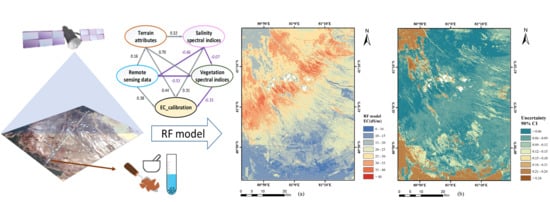
  • Overall, among the 35 factors considered, 9 indices (B6, B7, B10, B11, S6, GARI, GDVI, EVI, and DEM) were significant and contributed to the estimation of soil salinity. The random forest regression model was the best model in this study, with better model performance and accuracy measures (R2 = 0.75, RMSE = 7.33 dS m−1).
  • According to the EC map derived from the random forest model, the northwest and the south of the study area showed relatively low soil salinity. Salt was mainly concentrated in the northwest to the middle of the study area covering the desert.
  • Farmland reclamation affected the distribution of soil salinity, resulting in a strong positive correlation between elevation and soil EC. Moreover, the variability of soil salinity was sensitive to moisture and vegetation. Dry season was more conducive for the estimation of soil salinity.

Author Contributions

All authors had substantial contributions to this article. Conceptualization, N.W., J.P., and Z.S.; data curation, J.X., J.P., and Y.H.; formal analysis, N.W., J.X., and A.B.; funding acquisition, J.P. and Z.S.; methodology, N.W., A.B., and Y.H.; software, N.W., J.X., and J.P.; supervision, Z.S.; visualization, N.W., J.X., and J.P.; writing—original draft, N.W., J.P., and A.B. All authors have read and agreed to the published version of the manuscript.

Funding

This research was funded by the National Key Research and Development Program, grant number “2018YFE0107000”, and Young and Middle-aged Innovative Talents Program of Xinjiang production and Construction Crops, grant number “2020CB032”.

Conflicts of Interest

The funders had no role in the design of the study; in the collection, analyses, or interpretation of data; in the writing of the manuscript; or in the decision to publish the results.

References

  1. Wang, J.; Ding, J.; Yu, D.; Ma, X.; Zhang, Z.; Ge, X.; Teng, D.; Li, X.; Liang, J.; Lizaga, I.; et al. Capability of Sentinel-2 MSI data for monitoring and mapping of soil salinity in dry and wet seasons in the Ebinur Lake region, Xinjiang, China. Geoderma 2019, 353, 172–187. [Google Scholar] [CrossRef]
  2. Ren, D.; Wei, B.; Xu, X.; Engel, B.; Li, G.; Huang, Q.; Xiong, Y.; Huang, G. Analyzing spatiotemporal characteristics of soil salinity in arid irrigated agro-ecosystems using integrated approaches. Geoderma 2019, 356, 113935. [Google Scholar] [CrossRef]
  3. Gorji, T.; Sertel, E.; Tanik, A. Monitoring soil salinity via remote sensing technology under data scarce conditions: A case study from Turkey. Ecol. Indic. 2017, 74, 384–391. [Google Scholar] [CrossRef]
  4. Wicke, B.; Smeets, E.; Dornburg, V.; Vashev, B.; Gaiser, T.; Turkenburg, W.; Faaij, A. The global technical and economic potential of bioenergy from salt-affected soils. Energy Environ. Sci. 2011, 4, 2669–2681. [Google Scholar] [CrossRef] [Green Version]
  5. Ivushkin, K.; Bartholomeus, H.; Bregt, A.K.; Pulatov, A.; Kempen, B.; Sousa, L. Global mapping of soil salinity change. Remote Sens. Environ. 2019, 231, 111260. [Google Scholar] [CrossRef]
  6. Gorji, T.; Yildirim, A.; Hamzehpour, N.; Tanik, A.; Sertel, E. Soil salinity analysis of Urmia Lake Basin using Landsat-8 OLI and Sentinel-2A based spectral indices and electrical conductivity measurements. Ecol. Indic. 2020, 112, 106173. [Google Scholar] [CrossRef]
  7. Jiang, Q.; Peng, J.; Biswas, A.; Hu, J.; Zhao, R.; He, K.; Shi, Z. Characterising dryland salinity in three dimensions. Sci. Total Environ. 2019, 682, 190–199. [Google Scholar] [CrossRef]
  8. Ma, Z.; Zhou, L.; Yu, W.; Teng, H.; Shi, Z. Improving TMPA 3B43 V7 datasets using land surface characteristics and ground observations on the Qinghai-Tibet Plateau. Int. J. IEEE Geosci. Remote. Sens. Lett. 2018, 15, 178–182. [Google Scholar] [CrossRef]
  9. Shi, Z.; Cheng, J.; Huang, M.; Zhou, L. Assessing Reclamation Levels of Coastal Saline Lands with Integrated Stepwise Discriminant Analysis and Laboratory Hyperspectral Data. Pedosphere 2006, 16, 154–160. [Google Scholar] [CrossRef]
  10. Peng, J.; Ji, W.; Ma, Z.; Li, S.; Chen, S.; Zhou, L.; Shi, Z. Predicting total dissolved salts and soluble ion concentrations in agricultural soils using portable visible near-infrared and mid-infrared spectrometers. Biosyst. Eng. 2016, 152, 94–103. [Google Scholar] [CrossRef]
  11. Wu, W.; Muhaimeed, A.S.; Al-Shafie, W.M.; Al-Quraishi, A.M.F. Using L-band radar data for soil salinity mapping—a case study in Central Iraq. Environ. Res. Commun. 2019, 1, 081004. [Google Scholar] [CrossRef] [Green Version]
  12. Davis, E.; Wang, C.; Dow, K. Comparing Sentinel-2 MSI and Landsat 8 OLI in soil salinity detection: A case study of agricultural lands in coastal North Carolina. Int. J. Remote Sens. 2019, 40, 6134–6153. [Google Scholar] [CrossRef]
  13. Wang, J.; Ding, J.; Abulimiti, A.; Cai, L. Quantitative estimation of soil salinity by means of different modeling methods and visible-near infrared (VIS-NIR) spectroscopy, Ebinur Lake Wetland, Northwest China. PeerJ 2018, 6, e4703. [Google Scholar] [CrossRef] [PubMed] [Green Version]
  14. Vermeulen, D.; Van Niekerk, A. Machine learning performance for predicting soil salinity using different combinations of geomorphometric covariates. Geoderma 2017, 299, 1–12. [Google Scholar] [CrossRef]
  15. Dakak, H.; Huang, J.; Zouahri, A.; Douaik, A.; Triantafilis, J. Mapping soil salinity in 3-dimensions using an EM38 and EM4Soil inversion modelling at the reconnaissance scale in central Morocco. Soil Use Manag. 2017, 33, 553–567. [Google Scholar] [CrossRef]
  16. Hu, J.; Peng, J.; Zhou, Y.; Xu, D.; Zhao, R.; Jiang, Q.; Fu, T.; Shi, Z. Quantitative Estimation of Soil Salinity Using UAV-Borne Hyperspectral and Satellite Multispectral Images. Remote Sens. 2019, 11, 736. [Google Scholar] [CrossRef] [Green Version]
  17. Wang, X.; Zhang, F.; Ding, J.; Kung, H.; Latif, A.; Johnson, V.C. Estimation of soil salt content (SSC) in the Ebinur Lake Wetland National Nature Reserve (ELWNNR), Northwest China, based on a Bootstrap-BP neural network model and optimal spectral indices. Sci. Total Environ. 2018, 615, 918–930. [Google Scholar] [CrossRef]
  18. Mulder, V.L.; de Bruin, S.; Schaepman, M.E.; Mayr, T.R. The use of remote sensing in soil and terrain mapping—A review. Geoderma 2011, 162, 1–19. [Google Scholar] [CrossRef]
  19. McBratney, A.B.; Santos, M.L.M.; Minasny, B. On digital soil mapping. Geoderma 2003, 117, 3–52. [Google Scholar] [CrossRef]
  20. Jenny, H. Factors of Soil Formation; McGraw-Hill: New York, NY, USA, 1941. [Google Scholar]
  21. Bai, L.; Wang, C.; Zang, S.; Zang, S.; Wu, C.; Luo, J.; Wu, Y. Mapping Soil Alkalinity and Salinity in Northern Songnen Plain, China with the HJ-1 Hyperspectral Imager Data and Partial Least Squares Regression. Sensors 2018, 18, 3855. [Google Scholar] [CrossRef] [Green Version]
  22. Sultanov, M.; Ibrakhimov, M.; Akramkhanov, A.; Bauer, C.; Conrad, C. Modelling End-of-Season Soil Salinity in Irrigated Agriculture Through Multi-temporal Optical Remote Sensing, Environmental Parameters, and In Situ Information. PFG-J. Photogramm. Remote Sens. Geoinf. Sci. 2019, 86, 221–233. [Google Scholar] [CrossRef]
  23. Hoa, P.V.; Giang, N.V.; Binh, N.A.; Hai, L.V.H.; Phan, T.; Hasanlou, M.; Bui, D.T. Soil Salinity Mapping Using SAR Sentinel-1 Data and Advanced Machine Learning Algorithms: A Case Study at Ben Tre Province of the Mekong River Delta (Vietnam). Remote Sens. 2019, 11, 128. [Google Scholar] [CrossRef] [Green Version]
  24. Fathizad, H.; Ali, H.A.M.; Sodaiezadeh, H.; Kerry, R.; Taghizadeh-Mehrjardi, R. Investigation of the spatial and temporal variation of soil salinity using random forests in the central desert of Iran. Geoderma 2020, 365, 114233. [Google Scholar] [CrossRef]
  25. Masoud, A.A.; Koike, K.; Atwia, M.G.; El-Horiny, M.M.; Gemail, K.S. Mapping soil salinity using spectral mixture analysis of landsat 8 OLI images to identify factors influencing salinization in an arid region. Int. J. Appl. Earth Obs. 2019, 83, 101944. [Google Scholar] [CrossRef]
  26. Sanches, F.L.F.; Fernandes, A.C.P.; Ferreira, A.R.L.; Cortes, R.M.V.; Pacheco, F.A.L. A partial least squares - Path modeling analysis for the understanding of biodiversity loss in rural and urban watersheds in Portugal. Sci. Total Environ. 2018, 626, 1069–1085. [Google Scholar] [CrossRef]
  27. Ma, L.; Ma, F.; Li, J.; Ge, J.; Yang, S.; Wu, D.; Feng, J.; Ding, J. Characterizing and modeling regional-scale variations in soil salinity in the arid oasis of Tarim Basin, China. Geoderma 2017, 305, 1–11. [Google Scholar] [CrossRef]
  28. Peng, J.; Biswas, A.; Jiang, Q.; Zhao, R.; Hu, J.; Hu, B.; Shi, Z. Estimating soil salinity from remote sensing and terrain data in southern Xinjiang Province, China. Geoderma 2019, 337, 1309–1319. [Google Scholar] [CrossRef]
  29. Yang, R.M.; Guo, W.W. Using Sentinel-1 Imagery for Soil Salinity Prediction Under the Condition of Coastal Restoration. IEEE J. Sel. Top. Appl. Earth Obs. Remote Sens. 2019, 12, 1482–1488. [Google Scholar] [CrossRef]
  30. Chi, Y.; Sun, J.; Liu, W.; Wang, J.; Zhao, M. Mapping coastal wetland soil salinity in different seasons using an improved comprehensive land surface factor system. Ecol. Indic. 2017, 74, 384–391. [Google Scholar] [CrossRef]
  31. Yu, H.; Liu, M.; Du, B.; Wang, Z.; Hu, L.; Zhang, B. Mapping Soil Salinity/Sodicity by using Landsat OLI Imagery and PLSR Algorithm over Semiarid West Jilin Province, China. Sensors 2019, 107, 105517. [Google Scholar] [CrossRef] [Green Version]
  32. Wu, W.; Zucca, C.; Muhaimeed, A.S.; Ziadat, F.; Nangia, V.; Payne, W.B. Soil salinity prediction and mapping by machine learning regression in Central Mesopotamia, Iraq. Land Degrad. Dev. 2018, 29, 4005–4014. [Google Scholar] [CrossRef]
  33. Liu, Y.; Zhang, F.; Wang, C.; Wu, S.; Liu, J.; Xu, A.; Pan, K.; Pan, X. Estimating the soil salinity over partially vegetated surfaces from multispectral remote sensing image using non-negative matrix factorization. Geoderma 2019, 354, 113887. [Google Scholar] [CrossRef]
  34. Wang, F.; Shi, Z.; Biswas, A.; Yang, S.; Ding, J. Multi-algorithm comparison for predicting soil salinity. Geoderma 2020, 365, 114211. [Google Scholar] [CrossRef]
  35. Nouri, H.; Borujeni, S.C.; Alaghmand, S.; Anderson, S.J.; Sutton, P.C.; Parvazian, S.; Beecham, S. Soil Salinity Mapping of Urban Greenery Using Remote Sensing and Proximal Sensing Techniques; The Case of Veale Gardens within the Adelaide Parklands. Sustainability 2018, 10, 2826. [Google Scholar] [CrossRef] [Green Version]
  36. Wang, J.; Ding, J.; Yu, D.; Teng, D.; He, B.; Chen, X.; Ge, X.; Zhang, Z.; Wang, Y.; Yang, X.; et al. Machine learning-based detection of soil salinity in an arid desert region, Northwest China: A comparison between Landsat-8 OLI and Sentinel-2 MSI. Sci. Total Environ. 2020, 707, 136092. [Google Scholar] [CrossRef]
  37. Cheng, J.L.; Shi, Z.; Zhu, Y.W. Assessment and mapping of environmental quality in agricultural soils of Zhejiang Province, China. J. Environ. Sci. 2007, 19, 50–54. [Google Scholar] [CrossRef]
  38. Sabri, E.M.; Boukdir, A.; Karaoui, I.; Arioua, A.; Messlouhi, R.; Idrissi, A.E.A. Modelling soil salinity in Oued El Abid watershed, Morocco. E3S Web Conf. 2018, 37, 04002. [Google Scholar] [CrossRef] [Green Version]
  39. Taghadosi, M.M.; Hasanlou, M.; Eftekhari, K. Soil salinity mapping using dual-polarized SAR Sentinel-1 imagery. Int. J. Remote Sens. 2018, 40, 237–252. [Google Scholar] [CrossRef]
  40. Zhu, L.; Walker, J.P.; Tsang, L.; Huang, H.; Ye, N.; Rudiger, C. Soil moisture retrieval from time series multi-angular radar data using a dry down constraint. Remote Sens. Environ. 2019, 231, 111237. [Google Scholar] [CrossRef]
  41. Alifu, H.; Vuillaume, J.F.; Johnson, B.A.; Hirabayashi, Y. Machine-learning classification of debris-covered glaciers using a combination of Sentinel-1/-2 (SAR/optical), Landsat 8 (thermal) and digital elevation data. Geomorphology 2020, 369, 1–18. [Google Scholar] [CrossRef]
  42. Qiu, S.; Zhu, Z.; He, B. Fmask 4.0: Improved cloud and cloud shadow detection in Landsats 4–8 and Sentinel-2 imagery. Remote Sens. Environ. 2019, 231, 111205. [Google Scholar] [CrossRef]
  43. Muller, E.; DeÂcamps, H. Modeling soil moisture-reflectance. Remote Sens. Environ. 2000, 76, 173–180. [Google Scholar] [CrossRef] [Green Version]
  44. Taghizadeh-Mehrjardi, R.; Minasny, B.; Sarmadian, F.; Malone, B.P. Digital mapping of soil salinity in Ardakan region, central Iran. Geoderma 2014, 213, 15–28. [Google Scholar] [CrossRef]
  45. Huete, A.; Didan, K.; Miura, T.; Rodriguez, E.P.; Gao, X.; Ferreira, L.G. Overview of the radiometric and biophysical performance of the MODIS vegetation indices. Remote Sens. Environ. 2002, 83, 195–213. [Google Scholar] [CrossRef]
  46. Kumar, K.; Hari, P.K.S.; Arora, M.K. Estimation of water cloud model vegetation parameters using a genetic algorithm. Hydrol. Sci. J. 2012, 57, 776–789. [Google Scholar] [CrossRef] [Green Version]
  47. Douaoui, A.E.K.; Nicolas, H.; Walter, C. Detecting salinity hazards within a semiarid context by means of combining soil and remote-sensing data. Geoderma 2006, 134, 217–230. [Google Scholar] [CrossRef]
  48. Abbas, A.; Khan, S. Using Remote Sensing Techniques for Appraisal of Irrigated Soil Salinity. In Proceedings of International Congress on Modelling and Simulation; Oxley, L., Kulasiri, D., Eds.; Modelling & Simulation Soc Australia & New Zealand Inc.: Christchurch, New Zealand, 2007; pp. 2632–2638. [Google Scholar]
  49. Bannari, A.; Guedon, A.M.; El-Harti, A.; Cherkaoui, F.Z.; El-Chmari, A. Characterization of Slightly and Moderately Saline and Sodic Soils in Irrigated Agricultural Land using Simulated Data of Advanced Land Imaging (EO-1) Sensor. Commun. Soil Sci. Plant Anal. 2008, 39, 2795–2811. [Google Scholar] [CrossRef]
  50. Alexakis, D.D.; Daliakopoulos, I.N.; Panagea, I.S.; Tsanis, I.K. Assessing soil salinity using WorldView-2 multispectral images in Timpaki, Crete, Greece. Geocarto Int. 2016, 33, 321–338. [Google Scholar] [CrossRef]
  51. Gitelson, A.; Kaufman, Y.; Merzlyak, M. Use of a Green Channel in Remote Sensing of Global Vegetation from EOS-MODIS. Remote Sens. Environ. 1996, 58, 289–298. [Google Scholar] [CrossRef]
  52. Wu, W.; Al-Shafie, W.M.; Mhaimeed, A.S.; Ziadat, F.; Nangia, V.; Payne, W.B. Soil Salinity Mapping by Multiscale Remote Sensing in Mesopotamia, Iraq. IEEE J. Sel. Top. Appl. Earth Obs. Remote Sens. 2014, 7, 4442–4452. [Google Scholar] [CrossRef]
  53. Goel, N.S.; Qin, W. Influences of canopy architecture on relationships between various vegetation indices and LAI and Fpar: A computer simulation. Remote Sens. Rev. 1994, 10, 309–347. [Google Scholar] [CrossRef]
  54. Scudiero, E.; Skaggs, T.H.; Corwin, D.L. Regional scale soil salinity evaluation using Landsat 7, western San Joaquin Valley, California, USA. Geoderma Reg. 2014, 2–3, 82–90. [Google Scholar] [CrossRef]
  55. Zhang, X.; Huang, B. Prediction of soil salinity with soil-reflected spectra: A comparison of two regression methods. Sci. Rep. 2019, 9, 5067–5075. [Google Scholar] [CrossRef] [PubMed]
  56. Nurmemet, I.; Sagan, V.; Ding, J.; Halik, U.; Abliz, A.; Yakup, Z. A WFS-SVM Model for Soil Salinity Mapping in Keriya Oasis, Northwestern China Using Polarimetric Decomposition and Fully PolSAR Data. Remote Sens. 2018, 10, 598. [Google Scholar] [CrossRef] [Green Version]
  57. Ma, X.; Dai, Z.; He, Z.; Ma, J.; Wang, Y.; Wang, Y. Learning Traffic as Images: A Deep Convolutional Neural Network for Large-Scale Transportation Network Speed Prediction. Sensors 2017, 17, 818. [Google Scholar] [CrossRef] [PubMed] [Green Version]
  58. Alonso-Monsalve, S.; Suárez-Cetrulo, A.L.; Cervantes, A.; Quintana, D. Convolution on neural networks for high-frequency trend prediction of cryptocurrency exchange rates using technical indicators. Expert Syst. Appl. 2020, 149, 113250–113264. [Google Scholar] [CrossRef]
  59. Henseler, J.; Hubona, G.; Ray, P.A. Using PLS path modeling in new technology research: Updated guidelines. Ind. Manag. Data Syst. 2016, 116, 2–20. [Google Scholar] [CrossRef]
  60. Danks, N.; Sharma, P.; Sarstedt, M. Model selection uncertainty and multimodel inference in partial least squares structural equation modeling (PLS-SEM). J. Bus. Res. 2020, 113, 13–24. [Google Scholar] [CrossRef]
  61. Oliveira, C.F.; do Valle Junior, R.F.; Valera, C.A.; Rodrigues, V.S.; Fernandes, L.F.S.; Pacheco, F.A.L. The modeling of pasture conservation and of its impact on stream water quality using Partial Least Squares-Path Modeling. Sci. Total Environ. 2019, 697, 134081. [Google Scholar] [CrossRef]
  62. Huang, J.; Wu, J.; Fang, Y.; Wu, J.; Huang, J. Comparison of partial least square regression, support vector machine, and deep-learning techniques for estimating soil salinity from hyperspectral data. J. Appl. Remote Sens. 2018, 12, 022204. [Google Scholar]
  63. Pan, L.; Politis, D.N. Bootstrap prediction intervals for linear, nonlinear and nonparametric autoregressions. J. Stat. Plan. Inference 2016, 177, 1–27. [Google Scholar] [CrossRef] [Green Version]
  64. Zhou, Y.; Xue, J.; Chen, S.; Zhou, Y.; Liang, Z.; Wang, N.; Shi, Z. Fine-Resolution Mapping of Soil Total Nitrogen across China Based on Weighted Model Averaging. Remote Sens. 2020, 12, 85. [Google Scholar] [CrossRef] [Green Version]
  65. Fernández-Buces, N.; Siebe, C.; Cram, S.; Palacio, J.L. Mapping soil salinity using a combined spectral response index for bare soil and vegetation: A case study in the former lake Texcoco, Mexico. J. Arid Environ. 2006, 65, 644–667. [Google Scholar] [CrossRef]
  66. Zhang, T.; Qi, J.; Gao, Y.; Ouyang, Z.; Zeng, S.; Zhao, B. Detecting soil salinity with MODIS time series VI data. Ecol. Indic. 2015, 52, 480–489. [Google Scholar] [CrossRef]
  67. Shahabi, M.; Jafarzadeh, A.A.; Neyshabouri, M.R.; Ghorbani, M.A.; Kamran, K.V. Spatial modeling of soil salinity using multiple linear regression, ordinary kriging and artificial neural network methods. Arch. Agron. Soil Sci. 2016, 63, 151–160. [Google Scholar] [CrossRef]
  68. Ma, L.; Yang, S.; Simayi, Z.; Gu, Q.; Li, J.; Yang, X.; Ding, J. Modeling variations in soil salinity in the oasis of Junggar Basin, China. Land Degrad. Dev. 2018, 29, 551–562. [Google Scholar] [CrossRef]
  69. Patel, N.R.; Mukund, A.; Parida, B.R. Satellite-derived vegetation temperature condition index to infer root zone soil moisture in semi-arid province of Rajasthan, India. Geocarto Int. 2019, 1–17. [Google Scholar] [CrossRef]
  70. Hajj, M.E.; Baghdadi, N.; Zribi, M.; Belaud, G.; Cheviron, B.; Courault, D.; Charron, F. Soil moisture retrieval over irrigated grassland using X-band SAR data. Remote Sens. Environ. 2016, 176, 202–218. [Google Scholar] [CrossRef] [Green Version]
  71. Zhang, L.; Meng, Q.; Yao, S.; Wang, Q.; Zeng, J.; Zhao, S.; Ma, J. Soil Moisture Retrieval from the Chinese GF-3 Satellite and Optical Data over Agricultural Fields. Sensors 2018, 18, 2675. [Google Scholar] [CrossRef] [Green Version]
  72. Huang, J.; Koganti, T.; Santos, F.A.M.; Triantafilis, J. Mapping soil salinity and a fresh-water intrusion in three-dimensions using a quasi-3d joint-inversion of DUALEM-421S and EM34 data. Sci. Total Environ. 2017, 577, 395–404. [Google Scholar] [CrossRef]
  73. Schuberth, F.; Rademaker, M.E.; Henseler, J. Estimating and assessing second-order constructs using PLS-PM: The case of composites of composites. Ind. Manag. Data Syst. 2020, 120, 2211–2241. [Google Scholar] [CrossRef]
  74. Racetin, I.; Krtalic, A.; Srzic, V.; Zovko, M. Characterization of short-term salinity fluctuations in the Neretva River Delta situated in the southern Adriatic Croatia using Landsat-5 TM. Ecol. Indic. 2020, 110, 105924. [Google Scholar] [CrossRef]
  75. Thiam, S.; Villamor, G.B.; Kyei-Baffour, N.; Matty, F. Soil salinity assessment and coping strategies in the coastal agricultural landscape in Djilor district, Senegal. Land Use Policy 2019, 88, 104191. [Google Scholar] [CrossRef]
  76. Elia, S.; Todd, H.S.; Dennis, L.C. Regional-scale soil salinity assessment using Landsat ETM+ canopy reflectance. Remote Sens. Environ. 2015, 169, 335–343. [Google Scholar]
  77. Xu, H.; Chen, C.; Zheng, H.; Luo, G.; Yang, L.; Wang, W.; Wu, S.; Ding, J. AGA-SVR-based selection of feature subsets and optimization of parameter in regional soil salinization monitoring. Int. J. Remote Sens. 2020, 41, 4470–4495. [Google Scholar] [CrossRef]
  78. Ding, J.; Yu, D. Monitoring and evaluating spatial variability of soil salinity in dry and wet seasons in the Werigan–Kuqa Oasis, China, using remote sensing and electromagnetic induction instruments. Geoderma 2014, 235–236, 316–322. [Google Scholar] [CrossRef]
Figure 1. Geographical extent of the study area and the locations of sampling points. A total of 151 points were measured for soil electrical conductivity (EC) in two directions.
Remotesensing 12 04118 g001
Figure 2. Spatial distribution and violin plot of training and testing datasets.
Remotesensing 12 04118 g002
Figure 3. Uncertainty value of 48 testing points.
Remotesensing 12 04118 g003
Figure 4. Performance of EC estimation by (a) PLSR model, (b) CNN model, (c) SVM model, and (d) RF model by soil samples in bare soil (orange) and vegetation covered (green).
Remotesensing 12 04118 g004
Figure 5. EC map derived from random forest model (a) and uncertainty map of soil EC values (b).
Remotesensing 12 04118 g005
Figure 6. Importance of independent variables when modeling RF.
Remotesensing 12 04118 g006
Figure 7. Path analysis of training dataset.
Remotesensing 12 04118 g007
Table 1. Landsat-8 specifications for bands. Bands 1 to 9 are operational land imager (OLI) spectral bands and bands 10 and 11 are thermal infrared sensor (TIRS) spectral bands.
SensorSpectral BandWavelength (μm)Resolution (m)
OLIBand 1—Coastal/Aerosol0.433–0.45330
Band 2—Blue0.450–0.51530
Band 3—Green0.525–0.60030
Band 4—Red0.630–0.68030
Band 5—Near Infrared (NIR)0.845–0.88530
Band 6—Short Wavelength Infrared (SWIR)1.560–1.60030
Band 7—Short Wavelength Infrared (SWIR)2.100–2.30030
Band 8—Panchromatic0.500–0.68015
Band 9—Cirrus1.360–1.39030
TRISBand 10—Long Wavelength Infrared10.30–11.30100
Band 11—Long Wavelength Infrared11.50–12.50100
Table 2. Characteristics of Sentinel-1A data.
ParameterValue
Pass directionAscending
ModeInterferometric wide (IW)
PolarizationVH, VV
Temporal resolution12 days
Spatial resolution20 m
Wavelength5.6 cm
Radiometric stability0.5 dB (3ơ)
Radiometric accuracy1 dB (3ơ)
Phase error
Orbit number17,635
Swath250 km
Table 3. Thirty-five indices including auxiliary data (remote sensing data, terrain attributes, vegetation spectral indices, salinity spectral indices, and radar data) used to estimate soil EC in this study along with their abbreviations, calculation formulae, and the reference of calculation.
Auxiliary DataLand Surface ParametersAbbreviationFormulationsReferences
Remote sensing dataBands 1–7
Band 10
Band 11
B1–B7
B10
B11
Landsat-8
Brightness indexBI[(B4)2 + (B5)2]0.5[46]
Salinity spectral indicesSalinity indexSI(B4 × B2)0.5[46]
Salinity index 1SI1(B4 × B3)0.5[33]
Salinity index 3SI3[(B4)2 + (B3)2]0.5[33]
Salinity index IS1B2/B4[47]
Salinity index IIS2(B2 − B4)/(B2 + B4)[47]
Salinity index IIIS3B3 × B4/B2[48]
Salinity index IVS4B2 × B4/B3[48]
Salinity index VS5B4 × B5/B3[48]
Salinity index VIS6B6/B7[49]
Salinity index VIIS7(B6 − B7)/(B6 + B7)[49]
Salinity index VIIS8(B3 + B4)/2[47]
Salinity index IXS9(B3 + B4 + B5)/2[47]
Soil salinity indexSI_TB4/B5 × 100[50]
Vegetation spectral indicesNormalized difference vegetation indexNDVI(B5 − B4)/(B5 + B4)[51]
Green atmospherically resistant vegetation indexGARI{B5 − [B3 + γ × (B2 − B4)]}/{B5 + [B3 + γ × (B2 − B4)]}[51]
Extended NDVIENDVI(B5 + B7 − B4)/(B5 + B7 + B4)[36]
Generalized difference vegetation indexGDVI(B52 − B42)/(B52 + B42)[52]
Non-linear vegetation indexNLI(B52 − B4)/(B52 + B4)[53]
Canopy response salinity indexCRSI(B5 × B4 − B3 × B2)/(B5 × B4 + B3 × B2)0.5[52]
Enhanced vegetation indexEVIg × (B5 − B4)/(B5 + C1 × B4 − C2 × B2 + L)[54]
Terrain attributesElevationDEM [44]
SlopeS SAGA GIS
AspectA SAGA GIS
Radar dataBackscattering coefficients of VH bandVH0 − ơveg_VH0)/L[46]
Backscattering coefficients of VV bandVV0 − ơveg_VV0)/L[46]
Table 4. Descriptive statistics of EC (dSm−1).
DatasetsAmountMinMaxMeanMedianSDKutosisSkewnessCV
TrainingBare soil684.1044.8020.4717.409.760.561.0948%
Vegetation covered352.0946.7018.7714.5811.480.040.8561%
Entire datasets1032.0946.7019.8916.7310.350.270.9352%
TestingBare soil332.0942.6018.4516.439.570.270.7952%
Vegetation covered155.9041.5018.6116.378.513.281.5846%
Entire datasets482.0942.6018.5016.409.160.680.9450%
TotalBare soil1012.0944.8019.8116.739.700.460.9849%
Vegetation covered502.0946.7018.7215.7110.590.450.9657%
Entire study area1512.0946.7019.4516.679.980.390.9451%
Table 5. Correlation coefficients between 35 indices and measured EC values.
CategoryFactorRCategoryFactorR
Remote sensing dataB10.15Salinity spectral indicesS6−0.44 **
B20.19 *S70.03
B30.21 **S80.19 *
B40.14S90.19 *
B50.18 *SI_T−0.01
B60.26 **Vegetation spectral indicesNDVI−0.01
B70.23 **GARI−0.23 *
B100.40 **ENDVI0.09
B110.39 **GDVI−0.76 **
BI0.14NLI0.22 **
Salinity spectral indicesSI0.18 *CRSI−0.21 *
SI10.19 *EVI0.23 **
SI30.18 *Terrain attributesDEM0.41 **
S10.22 **S0.17 *
S20.22 **A−0.06
S30.14Radar dataVH−0.03
S40.14VV0.01
S5−0.04
** Significant at the 0.01 probability level. * Significant at the 0.05 probability level.
Table 6. Accuracy comparison of partial least squares regression (PLSR), convolutional neural network (CNN), support vector machine (SVM), and random forest (RF) models.
ModelsTotalBootstrapVegetation CoveredBare Soil
R2RMSER2RMSER2RMSER2RMSE
PLSR0.52 7.320.428.280.58 6.770.51 7.60
CNN0.53 6.440.547.980.51 6.13 0.54 6.58
SVM0.68 7.530.527.880.736.86 0.67 7.85
RF0.757.330.567.840.766.82 0.75 7.59
Publisher’s Note: MDPI stays neutral with regard to jurisdictional claims in published maps and institutional affiliations.

