Initial Assessment of the COSMIC-2/FORMOSAT-7 Neutral Atmosphere Data Quality in NESDIS/STAR Using In Situ and Satellite Data

 , ,
, ,
Abstract
:1. Introduction
2. Data
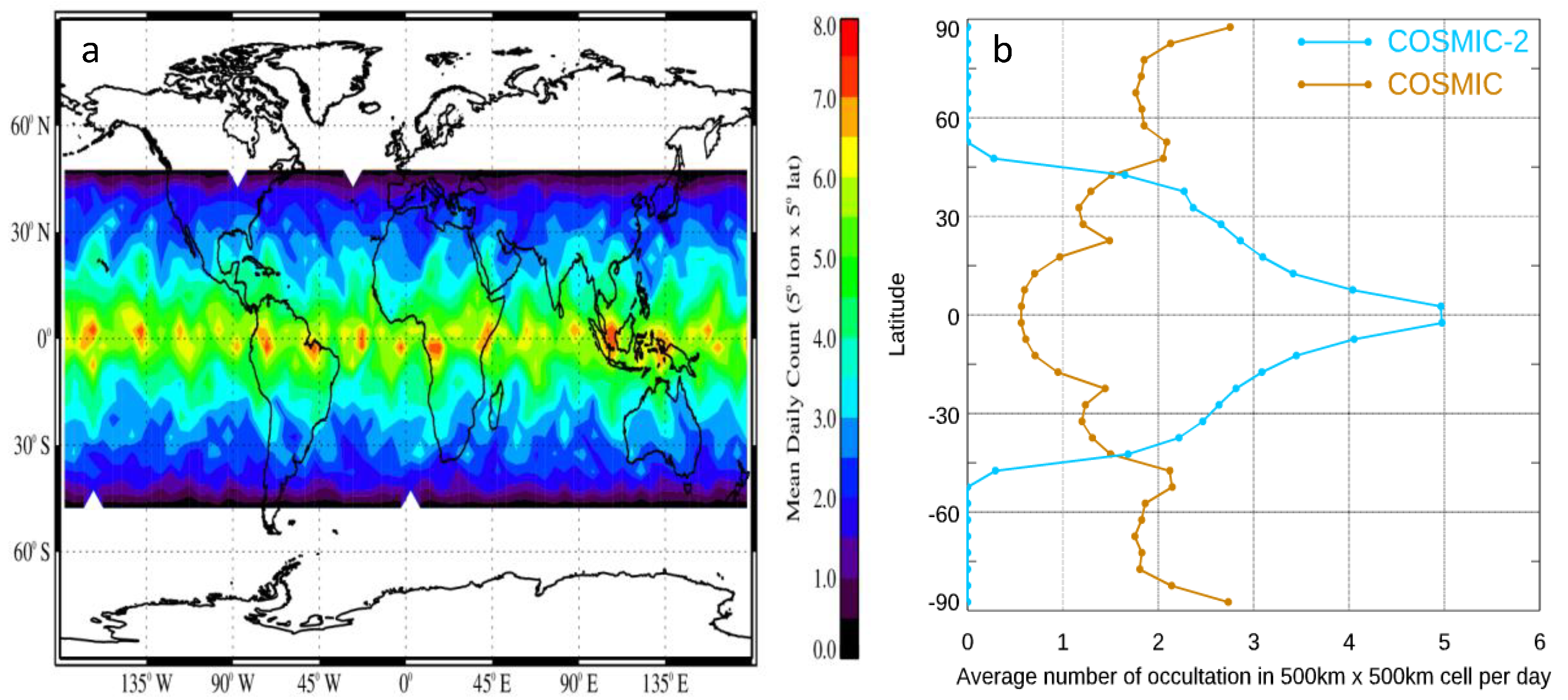
2.1. COSMIC-2 Data Coverage
2.2. CDAAC COSMIC-2 Neutral Atmospheric Profiles
2.3. RO Data from COSMIC, KOMPSAT 5, and MetOp-A,-B, -C GRAS, and TerraSAR-X
2.4. Radiosonde Data
3. Approaches for Quantifying the Precision, Stability, Accuracy, and Uncertainty of COSMIC-2 Data
4. Assessment of COSMIC-2 Penetration, Precision, and Stability
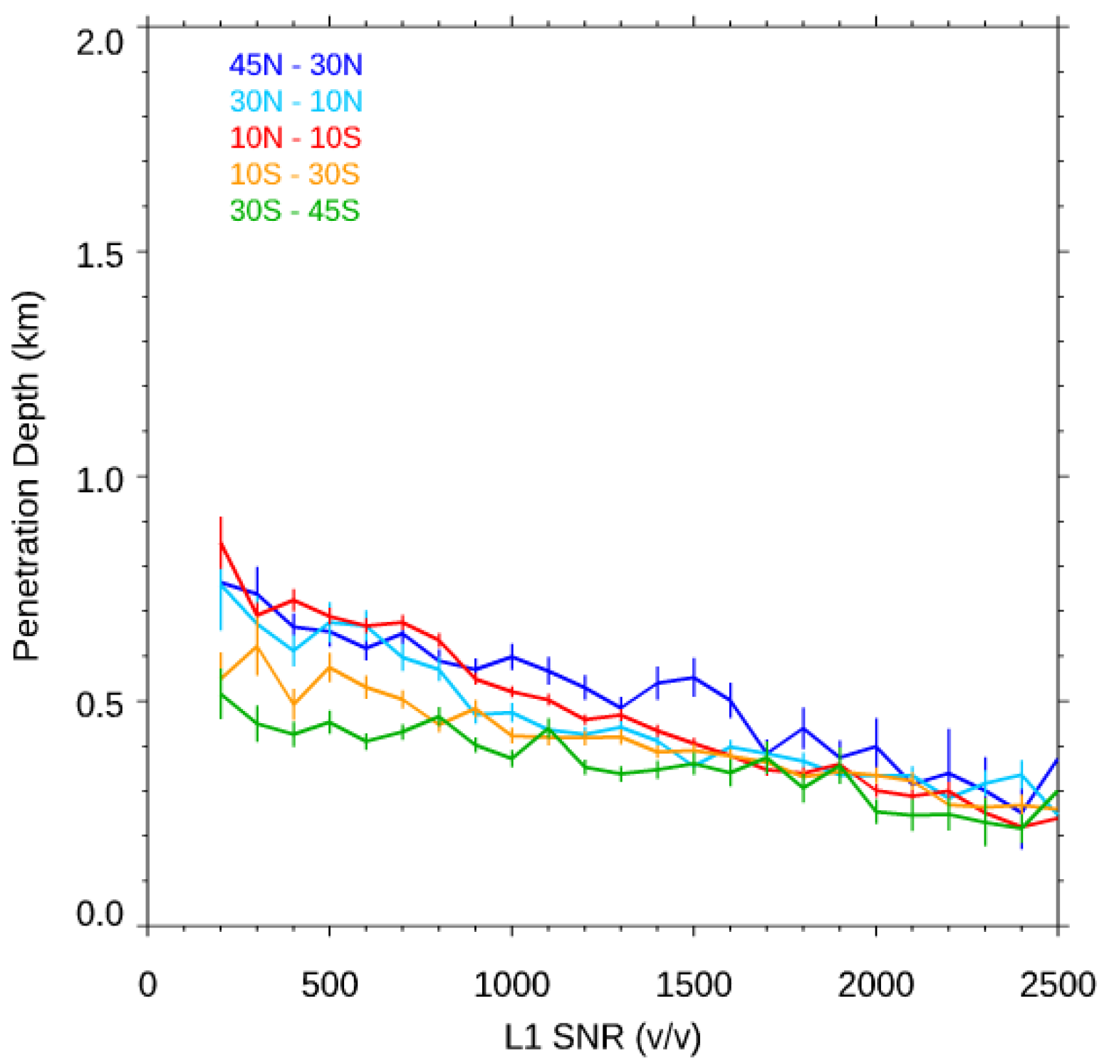
4.1. COSMIC-2 Penetration
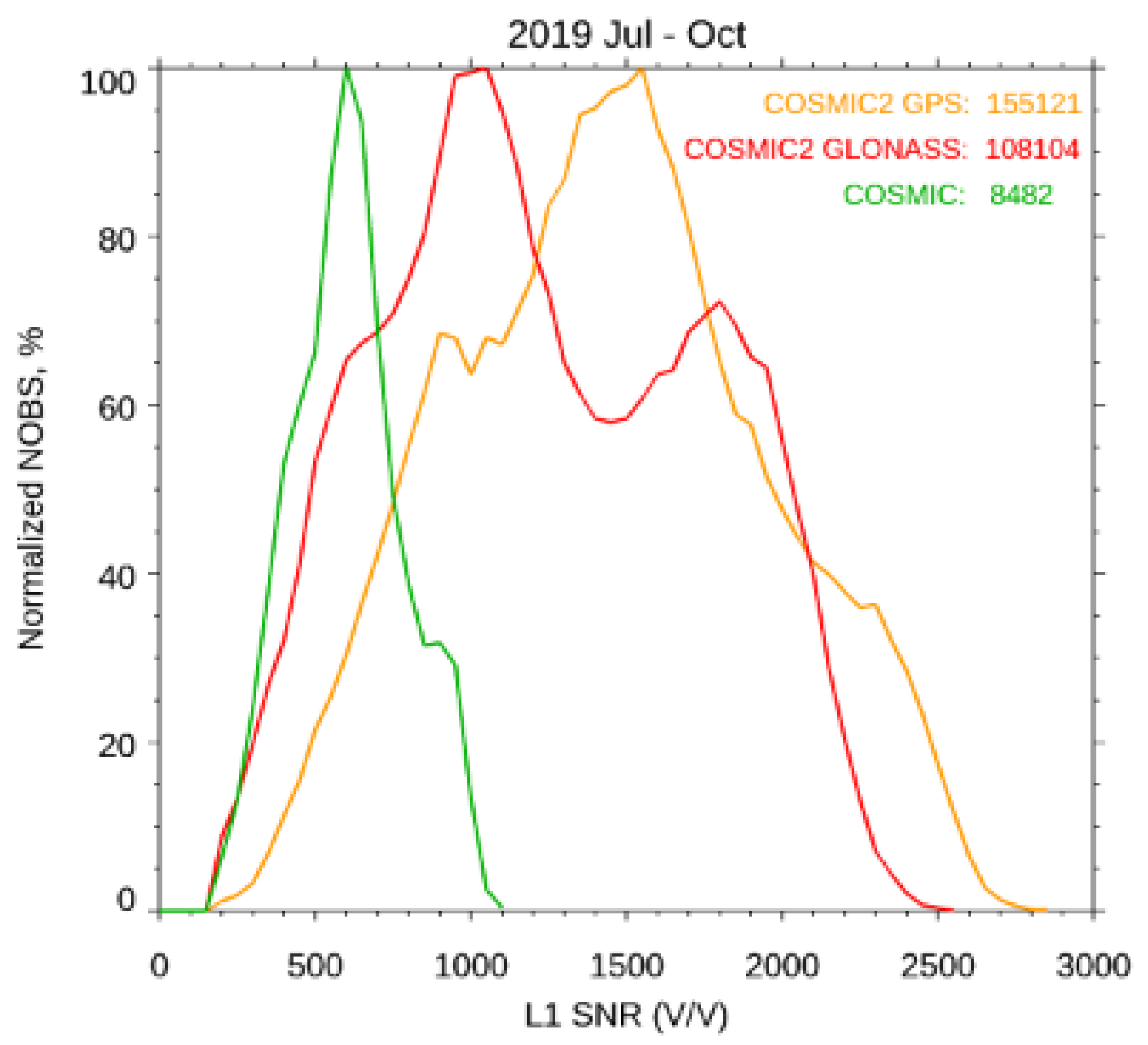
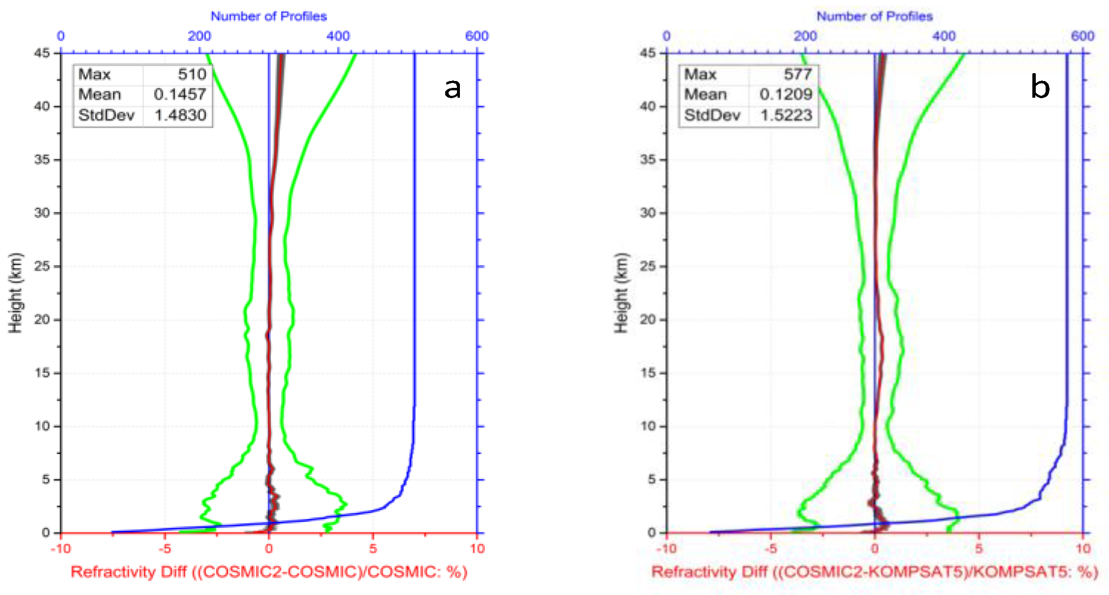
4.2. COSMIC-2 Precision
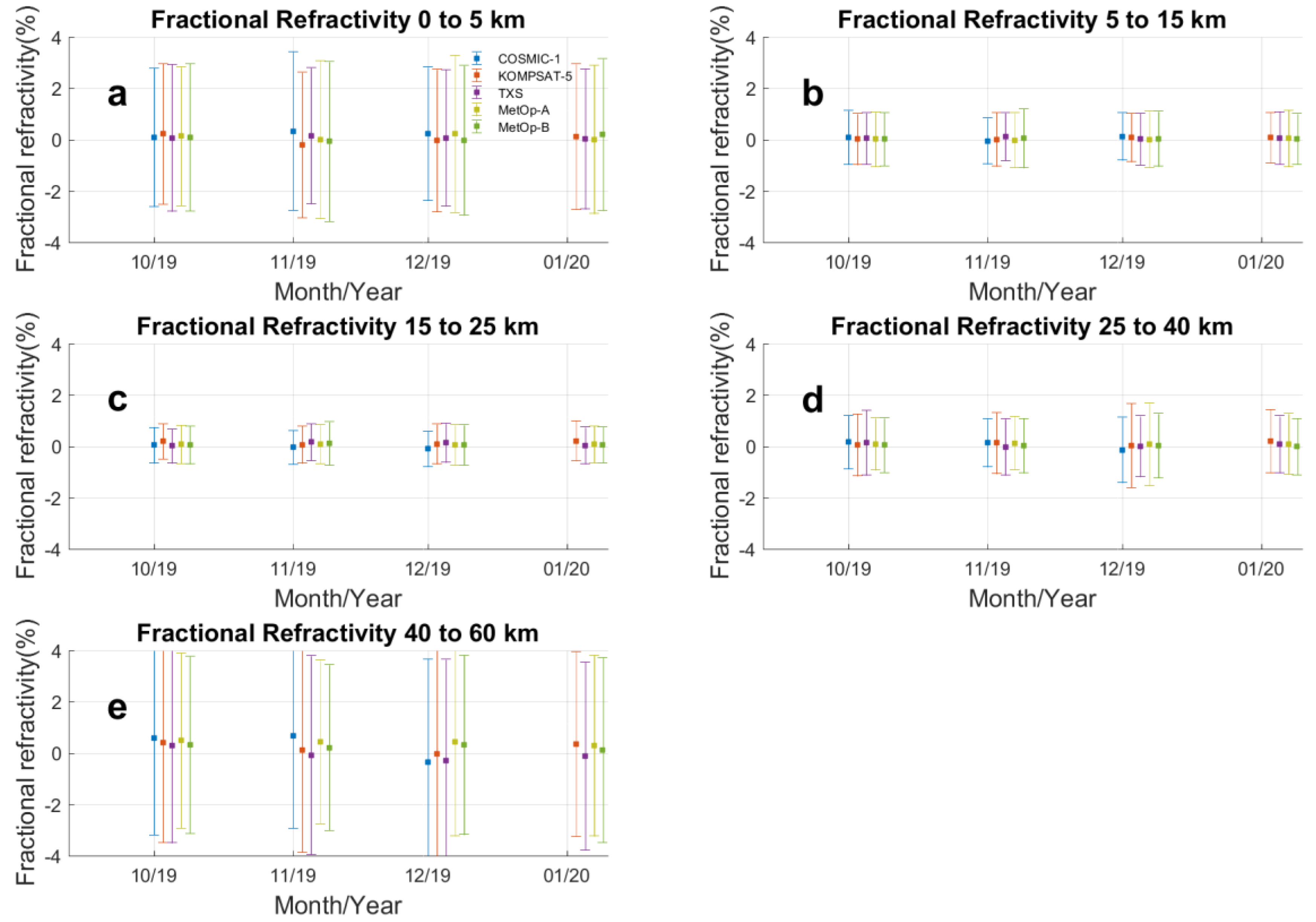
4.3. Stability Estimate
5. Accuracy and Uncertainty of COSMIC-2 Refractivity, Temperature, and Water Vapor Retrievals
5.1. General Quality of COSMIC-2 Refractivity and Water Vapor Profiles in the Lower Troposphere
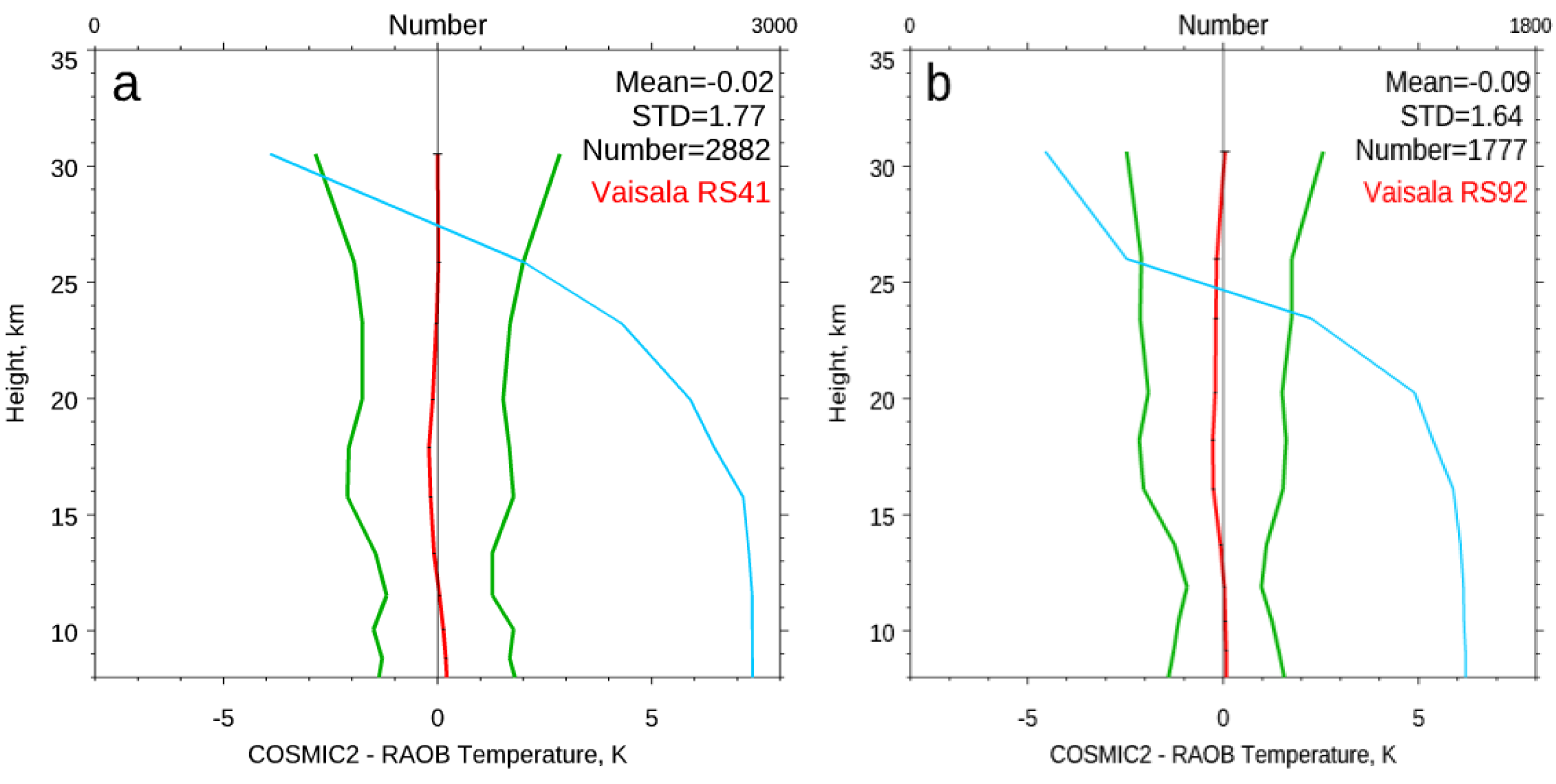
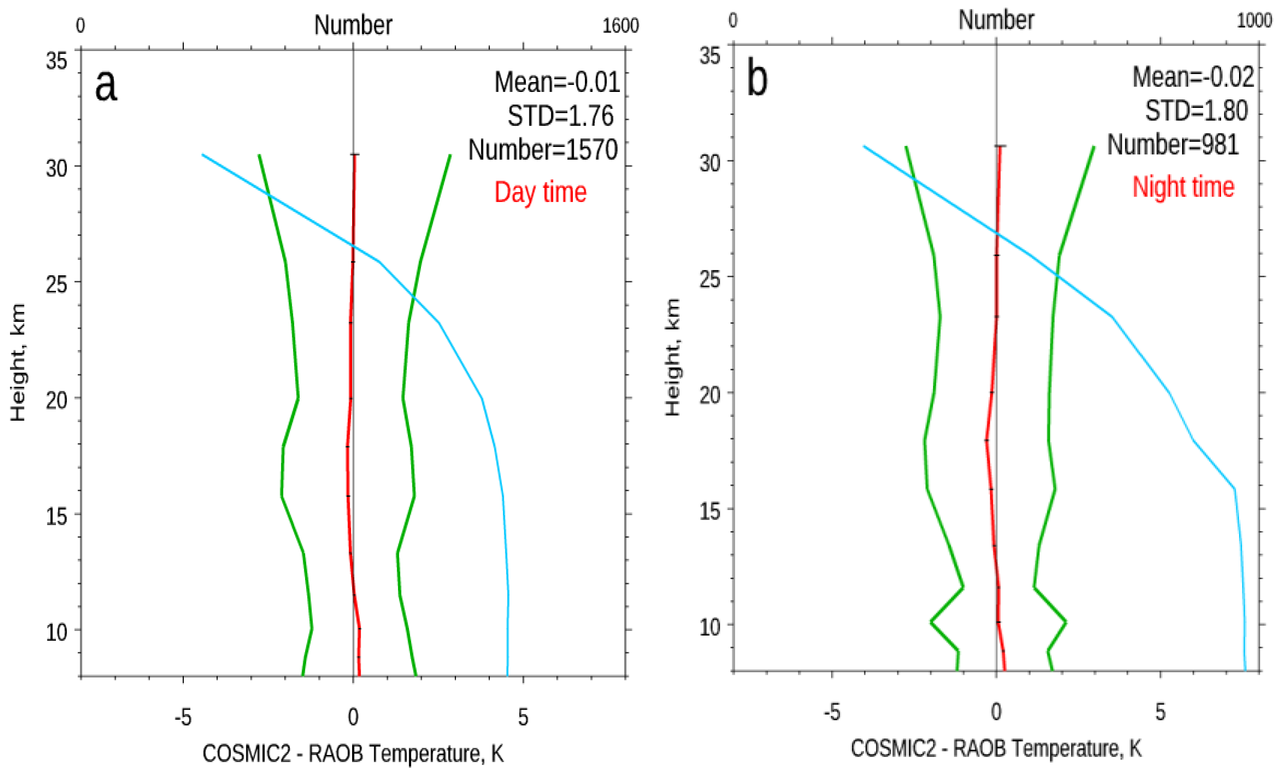
5.2. Accuracy and Uncertainty of COSMIC-2 Temperature in the Lower Stratosphere
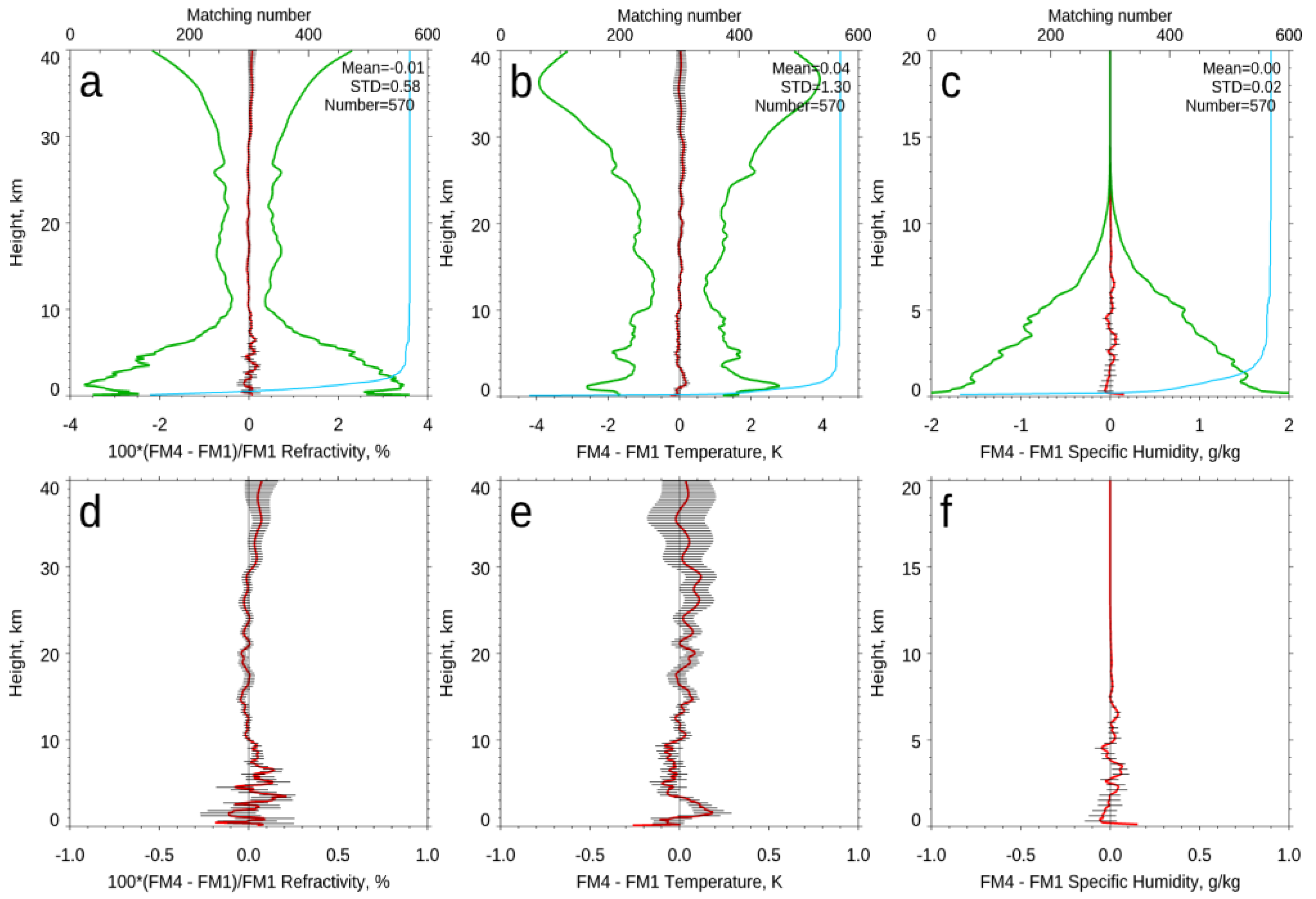
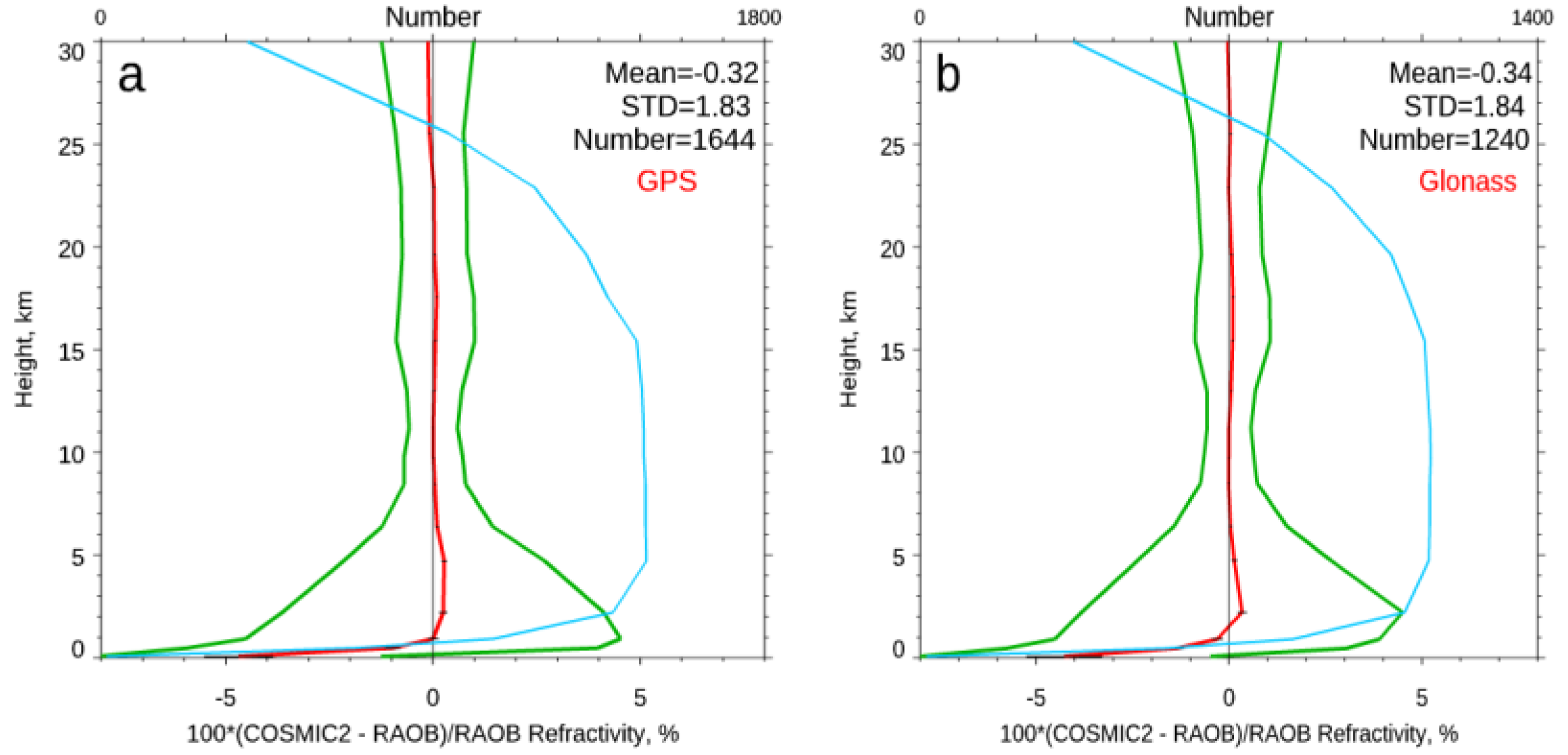
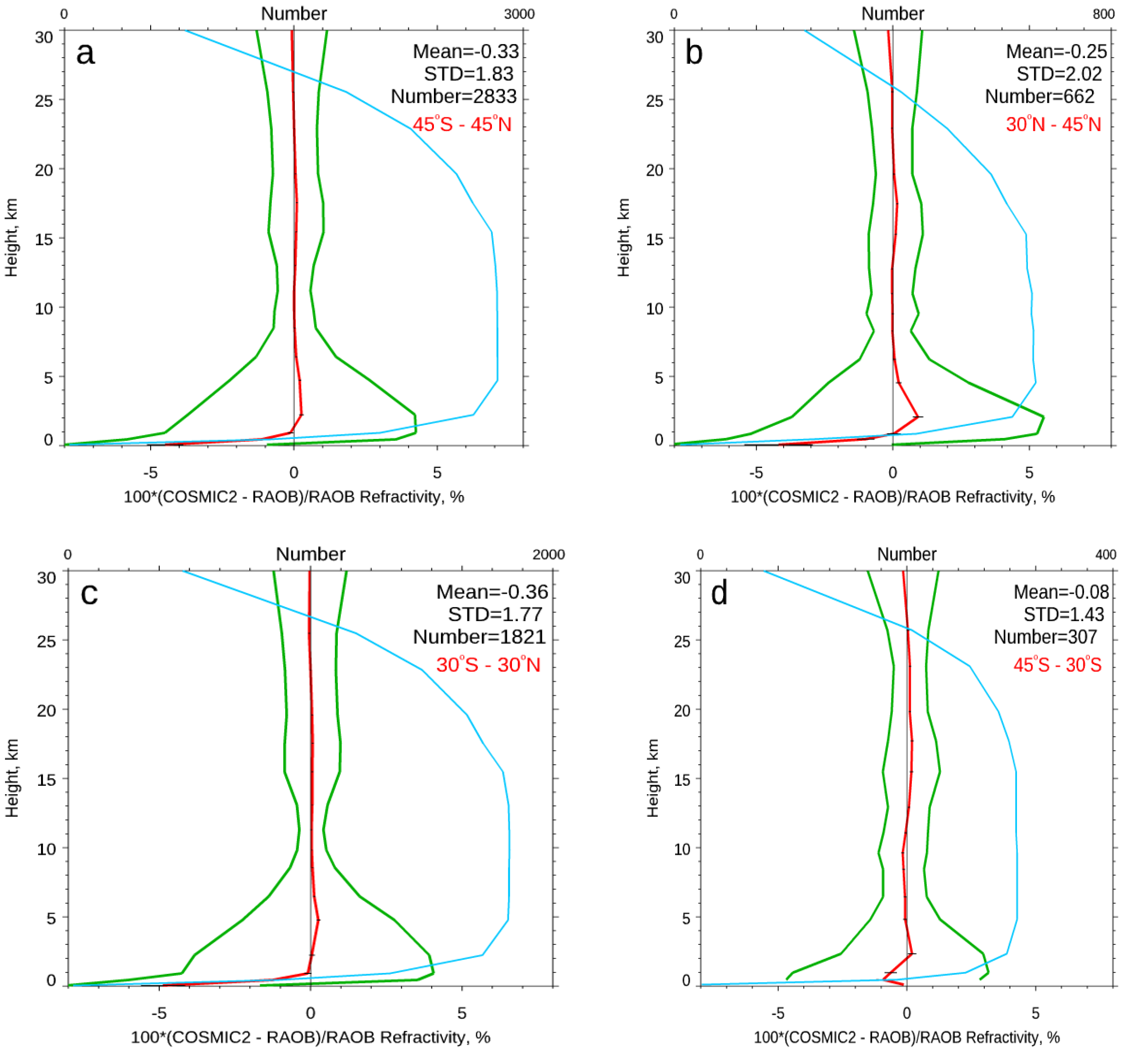
5.3. Accuracy and Uncertainty of COSMIC-2 Refractivity in the Troposphere
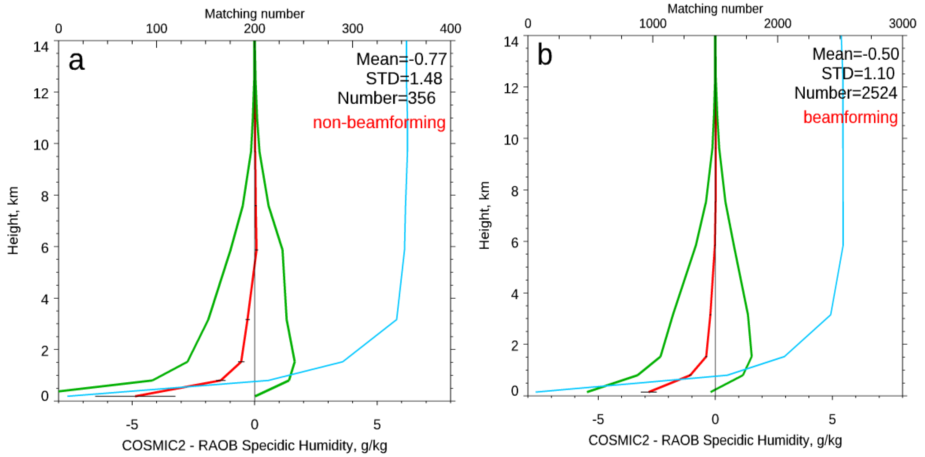
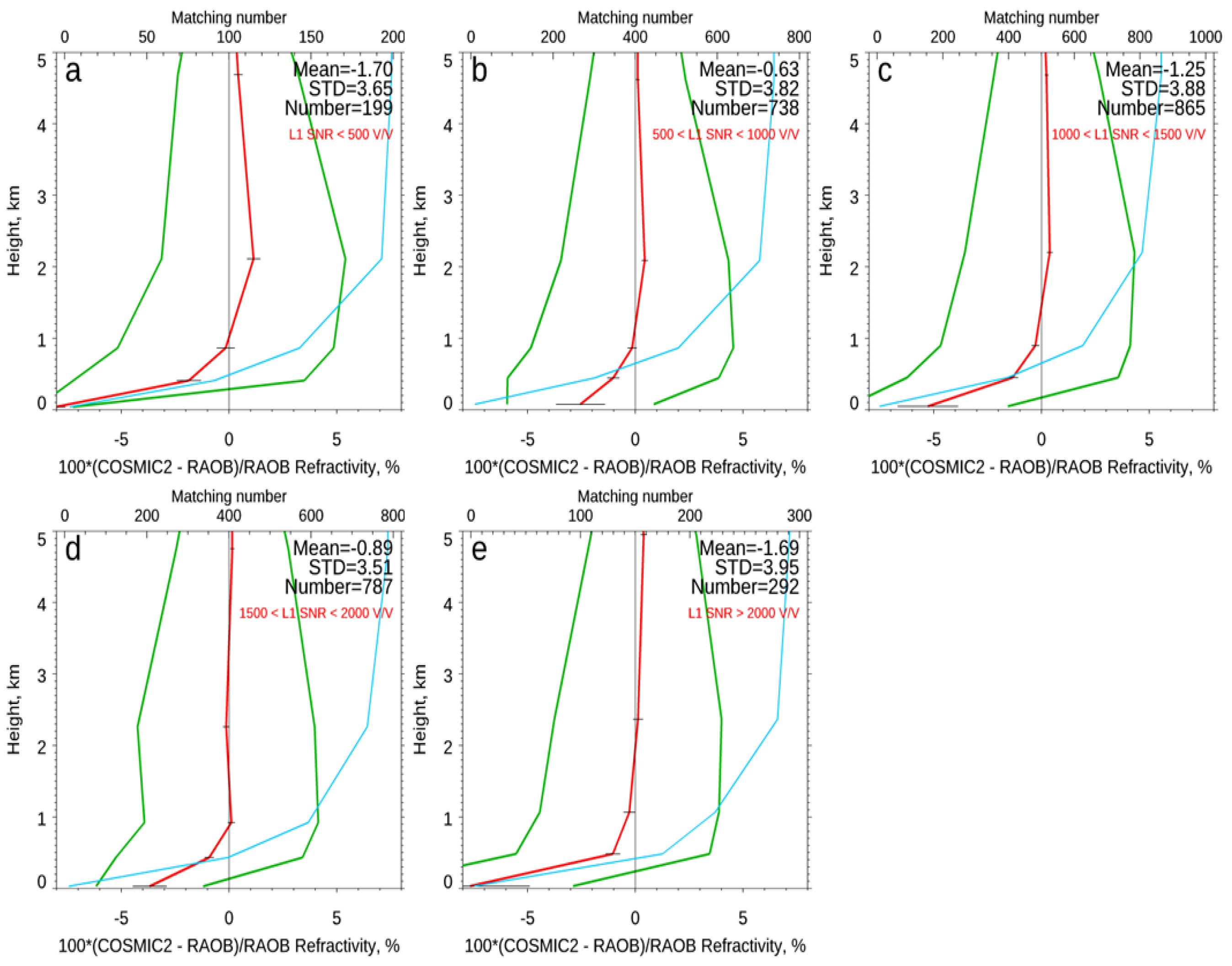
5.4. Accuracy and Uncertainty of COSMIC-2 Refractivity and Water Vapor Retrievals for Different SNR Groups
6. Conclusions, Discussions, and Potential Applications
Author Contributions
Funding
Acknowledgments
Conflicts of Interest
References
- Ho, S.-P.; Anthes, R.A.; Ao, C.O.; Healy, S.; Horanyi, A.; Hunt, D.; Mannucci, A.J.; Pedatella, N.; Randel, W.J.; Simmons, A.; et al. The COSMIC/FORMOSAT-3 Radio Occultation Mission after 12 Years: Accomplishments, Remaining Challenges, and Potential Impacts of COSMIC-2. Bull. Am. Meteorol. Soc. 2020, 101, E1107–E1136. [Google Scholar] [CrossRef] [Green Version]
- Zeng, Z.; Sokolovskiy, S.; Schreiner, W.S.; Hunt, D. Representation of Vertical Atmospheric Structures by Radio Occultation Observations in the Upper Troposphere and Lower Stratosphere: Comparison to High-Resolution Radiosonde Profiles. J. Atmos. Ocean. Technol. 2019, 36, 655–670. [Google Scholar] [CrossRef]
- Ho, S.-P.; Peng, L.; Mears, C.A.; Anthes, R.A. Comparison of global observations and trends of total precipitable water derived from microwave radiometers and COSMIC radio occultation from 2006 to 2013. Atmos. Chem. Phys. 2018, 18, 259–274. [Google Scholar] [CrossRef] [Green Version]
- Alexander, S.P.; Tsuda, T.; Kawatani, Y. COSMIC GPS Observations of Northern Hemisphere winter stratospheric gravity waves and comparisons with an atmospheric general circulation model. Geophys. Res. Lett. 2008, 35. [Google Scholar] [CrossRef]
- Alexander, S.P.; Tsuda, T.; Kawatani, Y.; Takahashi, M. Global distribution of atmospheric waves in the equatorial upper troposphere and lower stratosphere: COSMIC observations of wave mean flow interactions. J. Geophys. Res. Atmos. 2008, 113, D24115. [Google Scholar] [CrossRef]
- Luna, D.; Alexander, P.; De La Torre, A. Evaluation of uncertainty in gravity wave potential energy calculations through GPS radio occultation measurements. Adv. Space Res. 2013, 52, 879–882. [Google Scholar] [CrossRef]
- Nath, D.; Chen, W.; Guharay, A. Climatology of stratospheric gravity waves and their interaction with zonal mean wind over the tropics using GPS RO and ground-based measurements in the two phases of QBO. Theor. Appl. Clim. 2014, 119, 757–769. [Google Scholar] [CrossRef]
- Healy, S. Forecast impact experiment with a constellation of GPS radio occultation receivers. Atmos. Sci. Lett. 2008, 9, 111–118. [Google Scholar] [CrossRef]
- Healy, S. Surface pressure information retrieved from GPS radio occultation measurements. Q. J. R. Meteorol. Soc. 2013, 139, 2108–2118. [Google Scholar] [CrossRef]
- Aparicio, J.M.; Deblonde, G.; Aparicio, J.M. Impact of the Assimilation of CHAMP Refractivity Profiles on Environment Canada Global Forecasts. Mon. Weather Rev. 2008, 136, 257–275. [Google Scholar] [CrossRef]
- Poli, P.; Moll, P.; Puech, D.; Rabier, F.; Healy, S.B. Quality Control, Error Analysis, and Impact Assessment of FORMOSAT-3/COSMIC in Numerical Weather Prediction. Terr. Atmos. Ocean. Sci. 2009, 20, 101–113. [Google Scholar] [CrossRef] [Green Version]
- Cucurull, L. Improvement in the Use of an Operational Constellation of GPS Radio Occultation Receivers in Weather Forecasting. Weather Forecast. 2010, 25, 749–767. [Google Scholar] [CrossRef]
- Rennie, M.P. The impact of GPS radio occultation assimilation at the Met Office. Q. J. R. Meteorol. Soc. 2010, 136, 116–131. [Google Scholar] [CrossRef]
- Bonavita, M. On some aspects of the impact of GPSRO observations in global numerical weather prediction. Q. J. R. Meteorol. Soc. 2014, 140, 2546–2562. [Google Scholar] [CrossRef] [Green Version]
- Bauer, P.; Radnóti, G.; Healy, S.; Cardinali, C. GNSS Radio Occultation Constellation Observing System Experiments. Mon. Weather. Rev. 2014, 142, 555–572. [Google Scholar] [CrossRef]
- Anthes, R.A.; Bernhardt, P.A.; Chen, Y.; Cucurull, L.; Dymond, K.F.; Ector, D.; Healy, S.B.; Ho, S.-P.; Hunt, D.C.; Kuo, Y.; et al. The COSMIC/FORMOSAT-3 Mission: Early Results. Bull. Am. Meteorol. Soc. 2008, 89, 313–334. [Google Scholar] [CrossRef]
- Anthes, R.A. Exploring Earth’s atmosphere with radio occultation: Contributions to weather, climate and space weather. Atmos. Meas. Tech. 2011, 4, 1077–1103. [Google Scholar] [CrossRef] [Green Version]
- Adhikari, L.; Ho, S.-P. Inverting COSMIC-2 Phase Data to Bending Angle and Refractivity Profiles using the Full Spectrum Inversion Method. Remote Sens. 2020. Submitted. [Google Scholar]
- Zhang, B.; Ho, S.-P.; Shao, X. Bending Angle Inversion from Raw Observations of COSMIC-2. Remote Sens. 2020. Submitted. [Google Scholar]
- Kireev, S.; Ho, S.-P. COSMIC-2 1D Var inversion algorithm Water Vapor Retrievals in Tropical Moisture troposphere. Remote Sens. 2020. Submitted. [Google Scholar]
- Kuo, Y.-H.; Wee, T.-K.; Sokolovskiy, S.; Rocken, C.; Schreiner, W.; Hunt, D.; Anthes, R. Inversion and Error Estimation of GPS Radio Occultation Data. J. Meteorol. Soc. Jpn. 2004, 82, 507–531. [Google Scholar] [CrossRef] [Green Version]
- Ho, S.-P.; Kirchengast, G.; Leroy, S.; Wickert, J.; Mannucci, A.J.; Steiner, A.K.; Hunt, D.; Schreiner, W.; Sokolovskiy, S.; Ao, C.; et al. Estimating the uncertainty of using GPS radio occultation data for climate monitoring: Intercomparison of CHAMP refractivity climate records from 2002 to 2006 from different data centers. J. Geophys. Res. 2009, 114, D23107. [Google Scholar] [CrossRef] [Green Version]
- Ho, S.-P.; Hunt, D.; Steiner, A.K.; Mannucci, A.J.; Kirchengast, G.; Gleisner, H.; Heise, S.; Von Engeln, A.; Marquardt, C.; Sokolovskiy, S.; et al. Reproducibility of GPS radio occultation data for climate monitoring: Profile-to-profile inter-comparison of CHAMP climate records 2002 to 2008 from six data centers. J. Geophys. Res. 2012, 117, D18111. [Google Scholar] [CrossRef]
- Jensen, M.P.; Holdridge, D.J.; Survo, P.; Lehtinen, R.; Baxter, S.; Toto, T.; Johnson, K.L. Comparison of Vaisala radiosondes RS41 and RS92 at the ARM Southern Great Plains site. Atmos. Meas. Tech. 2016, 9, 3115–3129. [Google Scholar] [CrossRef] [Green Version]
- Melbourne, W.G.; Davis, E.S.; Duncan, C.B.; Hajj, G.A.; Hardy, K.R.; Kursinski, E.R.; Meehan, T.K.; Young, L.E.; Yunck, T.P. The Application of Spaceborne GPS to Atmospheric Limb Sounding and Global Change Monitoring; NASA Jet Propulsion Laboratory: Pasadena, CA, USA, 1994. Available online: https://ntrs.nasa.gov/archive/nasa/casi.ntrs.nasa.gov/19960008694.pdf (accessed on 17 June 2020).
- Yunck, T.P.; Liu, C.-H.; Ware, R. A History of GPS Sounding. Terr. Atmos. Ocean. Sci. 2000, 11, 001. [Google Scholar] [CrossRef] [Green Version]
- Smith, E.; Weintraub, S. The constants in the equation for atmospheric refractive index at radio frequencies. J. Res. Natl. Inst. Stand. Technol. 1953, 50, 39. [Google Scholar] [CrossRef]
- Neiman, P.J.; Ralph, F.M.; Wick, G.A.; Kuo, Y.-H.; Wee, T.-K.; Ma, Z.; Taylor, G.H.; Dettinger, M.D. Diagnosis of an Intense Atmospheric River Impacting the Pacific Northwest: Storm Summary and Offshore Vertical Structure Observed with COSMIC Satellite Retrievals. Mon. Weather Rev. 2008, 136, 4398–4420. [Google Scholar] [CrossRef] [Green Version]
- Wee, T.-K. A variational regularization of Abel transform for GPS radio occultation. Atmos. Meas. Tech. 2018, 11, 1947–1969. [Google Scholar] [CrossRef] [Green Version]
- Steiner, A.K.; Hunt, D.; Ho, S.-P.; Kirchengast, G.; Mannucci, A.J.; Scherllin-Pirscher, B.; Gleisner, H.; Von Engeln, A.; Schmidt, T.; Ao, C.; et al. Quantification of structural uncertainty in climate data records from GPS radio occultation. Atmos. Chem. Phys. Discuss. 2013, 13, 1469–1484. [Google Scholar] [CrossRef] [Green Version]
- Steiner, A.K.; Ladstädter, F.; Ao, C.O.; Gleisner, H.; Ho, S.-P.; Hunt, D.; Schmidt, T.; Foelsche, U.; Kirchengast, G.; Kuo, Y.-H.; et al. Consistency and structural uncertainty of multi-mission GPS radio occultation records. Atmos. Meas. Tech. 2020, 13, 2547–2575. [Google Scholar] [CrossRef]
- Ho, S.-P.; Peng, L.; Vömel, H. Characterization of the long-term radiosonde temperature biases in the upper troposphere and lower stratosphere using COSMIC and MetOp-A/GRAS data from 2006 to 2014. Atmos. Chem. Phys. Discuss. 2017, 17, 4493–4511. [Google Scholar] [CrossRef] [Green Version]
- Luers, J.K.; Eskridge, R.E. Use of Radiosonde Temperature Data in Climate Studies. J. Clim. 1998, 11, 1002–1019. [Google Scholar] [CrossRef]
- He, W.; Ho, S.-P.; Chen, H.; Zhou, X.; Hunt, D.; Kuo, Y.-H. Assessment of radiosonde temperature measurements in the upper troposphere and lower stratosphere using COSMIC radio occultation data. Geophys. Res. Lett. 2009, 36. [Google Scholar] [CrossRef] [Green Version]
- Motl, M. Vaisala RS41 trial in the Czech Republic. Vaisala News 2014, 192, 14–17. [Google Scholar]
- Jauhiainen, H.; Survo, P.; Lehtinen, R.; Lentonen, J. Radiosonde RS41 and RS92 key differences and comparison test results in different locations and climates. In Proceedings of the TECO-2014, WMO Technical Conference on Meteorological and Environmental Instruments and Methods of Observations, Saint Petersberg, Russia, 7–9 July 2014. [Google Scholar]
- Ao, C.O.; Meehan, T.; Hajj, G.A.; Mannucci, A.J.; Beyerle, G. Lower troposphere refractivity bias in GPS occultation retrievals. J. Geophys. Res. 2003, 108, 4577. [Google Scholar] [CrossRef] [Green Version]
- Sokolovskiy, S.V. Effect of super-refraction on inversions of radio occultation signals in the lower troposphere. Radio Sci. 2003, 38. [Google Scholar] [CrossRef] [Green Version]
- Xie, F.; Syndergaard, S.; Kursinski, E.R.; Herman, B.M. An Approach for Retrieving Marine Boundary Layer Refractivity from GPS Occultation Data in the Presence of Superrefraction. J. Atmos. Ocean. Technol. 2006, 23, 1629–1644. [Google Scholar] [CrossRef]
- Schreiner, W.S.; Weiss, J.; Anthes, R.; Braun, J.; Chu, V.; Fong, J.; Hunt, D.; Kuo, Y.; Meehan, T.; Serafino, W.; et al. COSMIC-2 Radio Occultation Constellation: First Results. Geophys. Res. Lett. 2020, 47, e2019GL086841. [Google Scholar] [CrossRef]
- Hajj, G.A.; Ao, C.O.; Iijima, B.A.; Kuang, D.; Kursinski, E.R.; Mannucci, A.J.; Meehan, T.; Romans, L.J.; Juárez, M.D.L.T.; Yunck, T.P. CHAMP and SAC-C atmospheric occultation results and intercomparisons. J. Geophys. Res. 2004, 109. [Google Scholar] [CrossRef]
- Ho, S.-P.; Goldberg, M.; Kuo, Y.-H.; Zou, C.-Z.; Shiau, W. Calibration of Temperature in the Lower Stratosphere from Microwave Measurements Using COSMIC Radio Occultation Data: Preliminary Results. Terr. Atmos. Ocean. Sci. 2009, 20, 87. [Google Scholar] [CrossRef] [Green Version]
- Kursinski, E.R.; Hajj, G.A.; Schofield, J.T.; Linfield, R.P.; Hardy, K.R. Observing Earth’s atmosphere with radio occultation measurements using the Global Positioning System. J. Geophys. Res. Space Phys. 1997, 102, 23429–23465. [Google Scholar] [CrossRef]
- Goody, R.; Anderson, J.; North, G. Testing Climate Models: An Approach. Bull. Am. Meteorol. Soc. 1998, 79, 2541–2549. [Google Scholar] [CrossRef] [Green Version]
- Ohring, G. Achieving Satellite Instrument Calibration for Climate Change (ASIC3); Workshop Rep.; NOAA: Camp Springs, MD, USA, 2007; 144p. Available online: www.star.nesdis.noaa.gov/star/documents/ASIC3-071218-webversfinal.pdf (accessed on 1 June 2020).
- Ho, S.-P.; Kuo, Y.-H.; Schreiner, W.; Zhou, X. Using SI-traceable global positioning system radio occultation measurements for climate monitoring [in “State of the Climate in 2009”]. Bull. Amer. Meteor. Soc. 2010, 91, S36–S37. [Google Scholar] [CrossRef]
- Sokolovskiy, S.; Schreiner, W.; Weiss, J.; Zeng, Z.; Hunt, D.; Braun, J. Initial Assessment of COSMIC-2 Data in the Lower Troposphere (LT) Joint 6th ROM SAF Data User Workshop and 7th IROWG Workshop; Konventum: Elsinore, Denmark, 2019. [Google Scholar]
- Gorbunov, M. The influence of the signal-to-noise ratio upon radio occultation inversion quality. Atmos. Meas. Tech. 2020. [Google Scholar] [CrossRef] [Green Version]
- Ho, S.-P.; Zhou, X.; Kuo, Y.-H.; Hunt, D.; Wang, J. Global Evaluation of Radiosonde Water Vapor Systematic Biases using GPS Radio Occultation from COSMIC and ECMWF Analysis. Remote Sens. 2010, 2, 1320–1330. [Google Scholar] [CrossRef] [Green Version]
- Ho, S.-P.; Yue, X.; Zeng, Z.; Ao, C.O.; Huang, C.-Y.; Kursinski, E.R.; Kuo, Y.-H. Applications of COSMIC Radio Occultation Data from the Troposphere to Ionosphere and Potential Impacts of COSMIC-2 Data. Bull. Am. Meteorol. Soc. 2014, 95. [Google Scholar] [CrossRef]
- Huang, C.-Y.; Teng, W.-H.; Ho, S.-P.; Kuo, Y.-H. Global variation of COSMIC precipitable water over land: Comparisons with ground-based GPS measurements and NCEP reanalyses. Geophys. Res. Lett. 2013, 40, 5327–5331. [Google Scholar] [CrossRef]
- Teng, W.-H.; Huang, C.-Y.; Ho, S.-P.; Kuo, Y.-H.; Zhou, X.-J. Characteristics of global precipitable water in ENSO events revealed by COSMIC measurements. J. Geophys. Res. Atmos. 2013, 118, 8411–8425. [Google Scholar] [CrossRef]
- Biondi, R.; Ho, S.-P.; Randel, W.; Syndergaard, S.; Neubert, T. Tropical cyclone cloud-top height and vertical temperature structure detection using GPS radio occultation measurements. J. Geophys. Res. Atmos. 2013, 118, 5247–5259. [Google Scholar] [CrossRef]
- Pirscher, B.; Deser, C.; Ho, S.; Chou, C.; Randel, W.; Kuo, Y. The vertical and spatial structure of ENSO in the upper troposphere and lower stratosphere from GPS radio occultation measurements. Geophys. Res. Lett. 2012, 39. [Google Scholar] [CrossRef] [Green Version]
- Zeng, Z.; Ho, S.-P.; Sokolovskiy, S.V.; Kuo, Y.-H. Structural evolution of the Madden-Julian Oscillation from COSMIC radio occultation data. J. Geophys. Res. 2012, 117, D22108. [Google Scholar] [CrossRef]
- Rieckh, T.; Anthes, R.; Randel, W.; Ho, S.-P.; Foelsche, U. Tropospheric dry layers in the tropical western Pacific: Comparisons of GPS radio occultation with multiple data sets. Atmos. Meas. Tech. 2017, 10, 1093–1110. [Google Scholar] [CrossRef] [Green Version]
- Schröder, M.; Lockhoff, M.; Shi, L.; August, T.; Bennartz, R.; Brogniez, H.; Calbet, X.; Fell, F.; Forsythe, J.; Gambacorta, A.; et al. The GEWEX Water Vapor Assessment: Overview and Introduction to Results and Recommendations. Remote Sens. 2019, 11, 251. [Google Scholar] [CrossRef] [Green Version]
- Biondi, R.; Randel, W.J.; Ho, S.-P.; Neubert, T.; Syndergaard, S. Thermal structure of intense convective clouds derived from GPS radio occultations. Atmos. Chem. Phys. 2012, 12, 5309–5318. [Google Scholar] [CrossRef] [Green Version]
- Xue, Y.H.; Li, J.; Menzel, P.; Borbas, E.; Ho, S.P.; Li, Z. Impact of Sampling Biases on the Global Trend of Total Precipitable Water Derived from the Latest 10-Year Data of COSMIC, SSMIS and HIRS Observations. J. Geophys. Res. Atmos. 2018, 124, 6966–6981. [Google Scholar]
- Mears, C.; Ho, S.-P.; Wang, J.; Peng, L. Total Column Water Vapor, [In “States of the Climate in 2017“]. Bul. Amer. Meteor. Sci. 2018, 99, S26–S27. [Google Scholar] [CrossRef]
- Mears, C.; Ho, S.-P.; Bock, O.; Zhou, X.; Nicolas, J. Total Column Water Vapor, [In “States of the Climate in 2018“]. Bul. Amer. Meteor. Sci. 2019, 100, S27–S28. [Google Scholar] [CrossRef] [Green Version]
- Ho, S.-P.; Peng, L.; Anthes, R.A.; Kuo, Y.-H.; Lin, H.-C. Marine Boundary Layer Heights and Their Longitudinal, Diurnal, and Interseasonal Variability in the Southeastern Pacific Using COSMIC, CALIOP, and Radiosonde Data. J. Clim. 2015, 28, 2856–2872. [Google Scholar] [CrossRef] [Green Version]


| 45° N–30° N | 30° N–10° N | 10° N–10° S | 10° S–30° S | 30° S–45° S | |
|---|---|---|---|---|---|
| COSMIC-2 0-500 v/v group | 1.2 | 1.2 | 1.3 | 1.2 | 0.8 |
| COSMIC-2 500-1000 v/v group | 1.1 | 0.9 | 1.2 | 0.9 | 0.7 |
| COSMIC-2 1000-1500 v/v group | 0.9 | 0.7 | 0.8 | 0.7 | 0.6 |
| COSMIC-2 1500-2000 v/v group | 0.8 | 0.5 | 0.5 | 0.5 | 0.5 |
| COSMIC-2 > 2000 v/v group | 0.6 | 0.4 | 0.3 | 0.4 | 0.4 |
| COSMIC-2 | 1.0 | 0.8 | 0.8 | 0.7 | 0.6 |
| COSMIC | 1.0 | 1.1 | 1.2 | 0.9 | 0.7 |
| KOMPSAT-5 | 1.0 | 1.2 | 1.3 | 0.9 | 0.6 |
| MetOp-A | 4.6 | 4.4 | 3.7 | 4.0 | 2.0 |
| MetOp-B | 3.1 | 3.4 | 3.3 | 4.4 | 1.9 |
| MetOp-C | 4.6 | 4.6 | 4.2 | 4.4 | 1.8 |
| Comparison Regions | 45° N to 45° S | North Hemisphere (45° N to 20° N) | Tropical Region (20° N–20° S) | Mid-Latitude South Hemisphere (20° S to 45° S) |
|---|---|---|---|---|
| Mean Difference (Stds) (%) | −0.33(1.83) | −0.25 (2.02) | −0.36(1.77) | −0.08 (1.43) |
| Sample number at 10 km altitude | 2833 | 662 | 1821 | 307 |
| L1 SNR Range | Mean Difference for Fractional Refractivity (std) from the Surface to 5 km Altitude (in %) | Sample Number at 5 km Altitude |
|---|---|---|
| 0–500 v/v | −1.7(3.65) | 199 |
| 500–1000 v/v | −0.63 (3.82) | 738 |
| 1000–1500 v/v | −1.25(3.88) | 865 |
| 1500–2000 v/v | −0.89(3.51) | 787 |
| >2000 v/v | −1.69(3.95) | 292 |
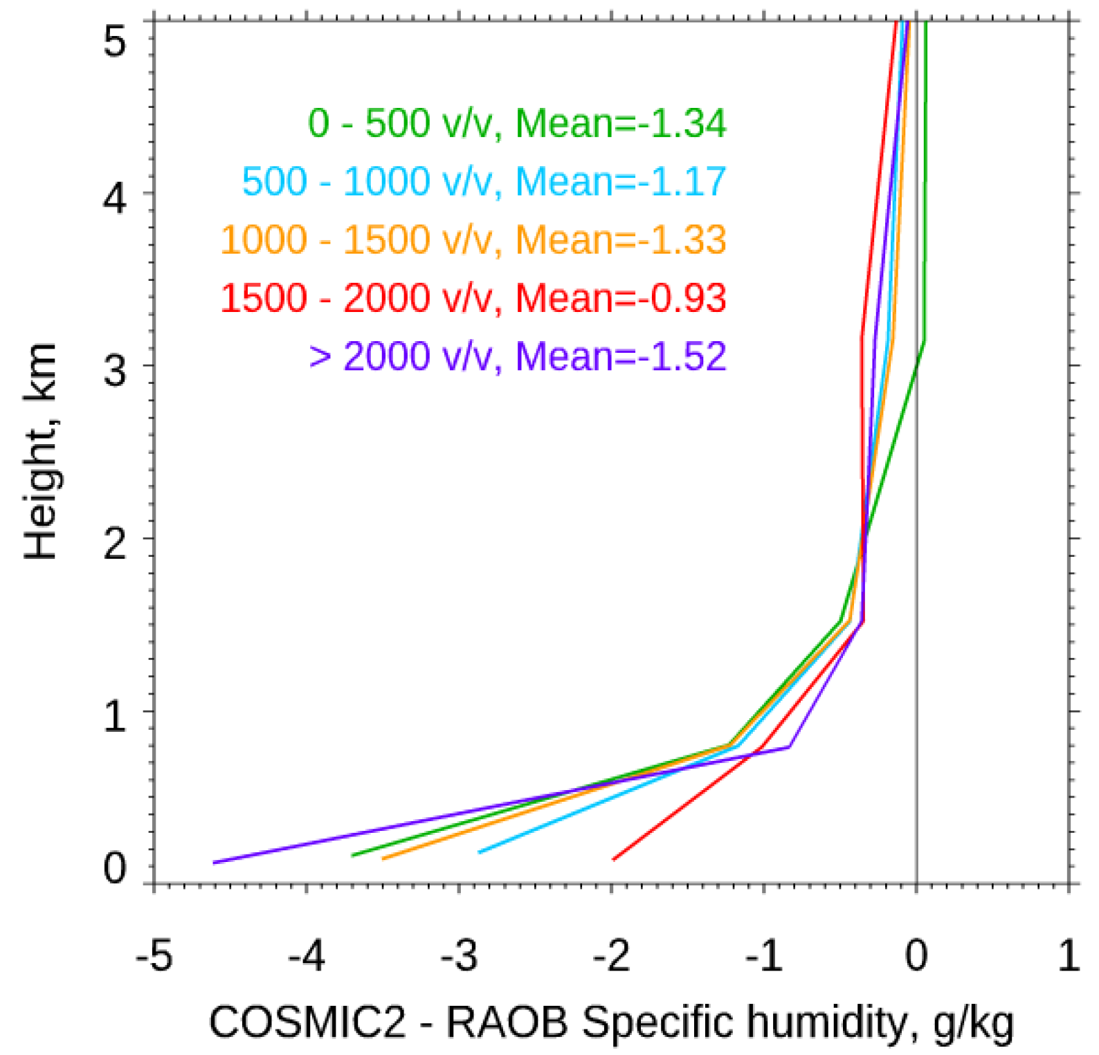
| L1 SNR Range | Mean Difference (stds) for Water Vapor from the Surface to 5 km Altitude (g/kg) |
|---|---|
| 0–500 v/v | −1.34 (2.51) |
| 500–1000 v/v | −1.17 (2.63) |
| 1000–1500 v/v | −1.33 (2.65) |
| 1500–2000 v/v | −0.93 (2.55) |
| >2000 v/v | −1.52 (2.62) |
Publisher’s Note: MDPI stays neutral with regard to jurisdictional claims in published maps and institutional affiliations. |
© 2020 by the authors. Licensee MDPI, Basel, Switzerland. This article is an open access article distributed under the terms and conditions of the Creative Commons Attribution (CC BY) license (http://creativecommons.org/licenses/by/4.0/).
Share and Cite
Ho, S.-P.; Zhou, X.; Shao, X.; Zhang, B.; Adhikari, L.; Kireev, S.; He, Y.; Yoe, J.G.; Xia-Serafino, W.; Lynch, E. Initial Assessment of the COSMIC-2/FORMOSAT-7 Neutral Atmosphere Data Quality in NESDIS/STAR Using In Situ and Satellite Data. Remote Sens. 2020, 12, 4099. https://doi.org/10.3390/rs12244099
Ho S-P, Zhou X, Shao X, Zhang B, Adhikari L, Kireev S, He Y, Yoe JG, Xia-Serafino W, Lynch E. Initial Assessment of the COSMIC-2/FORMOSAT-7 Neutral Atmosphere Data Quality in NESDIS/STAR Using In Situ and Satellite Data. Remote Sensing. 2020; 12(24):4099. https://doi.org/10.3390/rs12244099
Chicago/Turabian StyleHo, Shu-Peng, Xinjia Zhou, Xi Shao, Bin Zhang, Loknath Adhikari, Stanislav Kireev, Yuxiang He, James G. Yoe, Wei Xia-Serafino, and Erin Lynch. 2020. "Initial Assessment of the COSMIC-2/FORMOSAT-7 Neutral Atmosphere Data Quality in NESDIS/STAR Using In Situ and Satellite Data" Remote Sensing 12, no. 24: 4099. https://doi.org/10.3390/rs12244099