Article

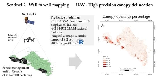
Mapping of the Canopy Openings in Mixed Beech–Fir Forest at Sentinel-2 Subpixel Level Using UAV and Machine Learning Approach

1
Croatian Forest Research Institute, Division of Ecology, Cvjetno naselje 41, 10450 Jastrebarsko, Croatia
2
Faculty of Geodesy, University of Zagreb, Kačićeva 26, 10000 Zagreb, Croatia
3
Croatian Forests Ltd., Ivana Meštrovića 28, 48000 Koprivnica, Croatia
*
Author to whom correspondence should be addressed.
Remote Sens. 2020, 12(23), 3925; https://doi.org/10.3390/rs12233925
Submission received: 30 October 2020 / Revised: 22 November 2020 / Accepted: 27 November 2020 / Published: 30 November 2020

Abstract

:
The presented study demonstrates a bi-sensor approach suitable for rapid and precise up-to-date mapping of forest canopy gaps for the larger spatial extent. The approach makes use of Unmanned Aerial Vehicle (UAV) red, green and blue (RGB) images on smaller areas for highly precise forest canopy mask creation. Sentinel-2 was used as a scaling platform for transferring information from the UAV to a wider spatial extent. Various approaches to an improvement in the predictive performance were examined: (I) the highest R2 of the single satellite index was 0.57, (II) the highest R2 using multiple features obtained from the single-date, S-2 image was 0.624, and (III) the highest R2 on the multitemporal set of S-2 images was 0.697. Satellite indices such as Atmospherically Resistant Vegetation Index (ARVI), Infrared Percentage Vegetation Index (IPVI), Normalized Difference Index (NDI45), Pigment-Specific Simple Ratio Index (PSSRa), Modified Chlorophyll Absorption Ratio Index (MCARI), Color Index (CI), Redness Index (RI), and Normalized Difference Turbidity Index (NDTI) were the dominant predictors in most of the Machine Learning (ML) algorithms. The more complex ML algorithms such as the Support Vector Machines (SVM), Random Forest (RF), Stochastic Gradient Boosting (GBM), Extreme Gradient Boosting (XGBoost), and Catboost that provided the best performance on the training set exhibited weaker generalization capabilities. Therefore, a simpler and more robust Elastic Net (ENET) algorithm was chosen for the final map creation.

Graphical Abstract

1. Introduction

Forest canopy gaps, as a consequence of management activities or natural disturbances, are the main drivers that affect forest dynamics in most continuous-cover, close-to-nature silvicultural systems. Gap-based interventions to create a more open-stand structure represent common silvicultural practices for regeneration, as well as forest exploitation in the mixed silver fir (Abies alba Mill.) and European beech (Fagus sylvatica L.) forests in Central Europe. The size and position of crown openings determine the amount of direct light able to penetrate to the forest floor, thus creating conditions that could favor the shade-tolerant silver fir or the regeneration of the more competitive European beech in conditions of supplementary light availability [1]. The creation of treefall gaps accelerates tree regeneration and increases tree species diversity in mixed beech–fir forests [2]. The creation of canopy openings through natural tree mortality processes, wind-driven gap formation, or manmade activities also has a significant influence on changes in microclimatic conditions and below-ground processes. Canopy openings have an impact on increases in air and soil temperatures and decreases in soil moisture in larger gaps [3]. Humification processes prevail in small gaps, i.e., an increase in soil organic content, while, in large gaps, the mineralization processes related to decreases in organic content are more dominant [4,5]. The questions of size, shape, and topographic position of forest openings have been extensively studied [6,7,8,9,10,11,12,13]. They have been done so as to emulate the natural disturbance processes and to discover the most appropriate silvicultural operations that would imitate natural regeneration, particularly with the aim of conversion of various monocultures toward close-to-nature forests [14].
The estimation of forest canopy gaps or openings is commonly obtained from measures of canopy cover that can be defined as a percentage of forest area occupied by the vertical projection of tree crowns, unlike the canopy closure that has an analogous meaning but is represented by the proportion of sky hemisphere obscured by vegetation when viewed from a single point. There are three different groups of approaches [15] for measuring or estimating the crown canopy density in a forest: (I) ground measurement at the study area, (II) statistical approaches, if the information such as basal area or diameter at breast height and the number of trees per area is available, and (III) remote sensing data such as aerial photographs, satellite data, or laser scanner data. When making ground measurements, devices such as densiometers and hemispherical digital photographs are used or they are based on pure ocular assessment [16,17]. Ground measurement methods, as the most accurate techniques, are labor-intensive and cannot rapidly provide canopy cover estimates [17]. Recently, remote sensing methods, in particular light detection and ranging (LiDAR), have been proven as the most advantageous approaches in terms of accuracy and ease of data acquisition [18,19,20,21]. UAV (unmanned aerial vehicle)-based LiDAR, despite observed shortcomings such as aircraft instability, is lower in cost, more convenient in terms of operation, and has a more flexible flight route design, as well as unique advantages in the possibilities of better discernment of the stand canopy details than airborne LiDAR [19]. Satellite remote sensing, medium-resolution data from Landsat are traditionally a very appropriate source of information for crown cover estimation, most often comprising the supervised classification approaches based on ground truth validation sets obtained from field measurements, airborne or UAV aero-photo imagery, and LiDAR or very high-resolution satellite imagery [22,23,24,25,26,27,28]. The main drawback of medium-resolution satellite data such as Landsat 8 is that its spatial resolution of 30 m is too coarse for precise forest gap detection. One of the most prominent examples of canopy closure estimation worth mentioning is tree cover density product in 20 m resolution, developed for the Pan-European scale in 2012, 2015, and 2018, as part of the Copernicus Land Monitoring Service [29].
By launching a pair of Sentinel-2 satellites in 2015 and 2017, the European Space Agency (ESA) made a considerable breakthrough in improving the ability of the global monitoring of conditions and changes in forest cover primarily due to cost-free data availability, as well as highly advanced sensor characteristics: very good spectral properties (13 bands from 492.1 to 2185.7 nm, central wavelengths), radiometric resolution (12 bit; a potential range of brightness levels from 0–4095), spatial resolution (10 m for read, green, blue and near infra red bands), and revisit time (5 days under cloud-free conditions) [30]. These characteristics enable improved monitoring of the conditions and changes in the land cover and its dynamics on a global scale. Sentinel 2 Multispectral Instrument (MSI) with a 10 m spatial resolution shows some improvement in the possibility of detection of selective logging gaps in relation to Landsat 8 [31,32,33]. On the other hand, the possibilities of the employment of Sentinel 2 in operational forestry to its full performance have not been fully recognized and valorized up to the present. Apparently, a major disadvantage of the Sentinel 2 MSI sensor, which limits its greater use in forestry, is its 10 m spatial resolution which prevents exact geolocation and delineation of individual trees, which is important for many silvicultural practices; for this reason, other more precise survey methods such as LiDAR, UAV images, and very high resolution satellite imagery are often more attractive and competitive. Finer spatial resolution is especially important in the management of uneven-aged mixed forests where silvicultural interventions take place at the level of an individual tree or a smaller group of trees, and we rarely find larger interrupted areas (except in the case of natural disasters such as windbreaks or ice breaks) that can be clearly identified on satellite Sentinel 2 or Landsat 8 images [34].
For the successful implementation of remote sensing products in operational forestry, several prerequisites need to be met, related to their compliance on the scale of which the various forest management planning activities are carried out. Given the temporal scale, we can usually distinguish medium-term forest management planning, usually on a decadal time scale, on the basis of the conducted forest inventory. In addition, there is more operational, annual planning that requires more current, timely information from the forests according to which operational silvicultural decisions are implemented in the short term. In the case of continuous-cover mixed forests, it is of great importance to mark locations within the forest stand with an overly dense canopy structure where a selective cut for regeneration purposes or thinning should be carried out. Further information on the location of newly created forest gaps, after a natural disaster, windbreak, ice breakage, or biotic damages, can be used in the planning of the restoration of these areas, construction of the logging trails, calculation of the man-hours of the forest workers and machines, etc. Regarding the spatial scale, the extent of the supporting data layer should comply with the extent of the forest area that is considered in the operational planning, usually on the scale of the forest managerial unit. In Croatia, with the usual size being between 3000 and 6000 hectares, the forest managerial units (FMUs) are the lowest organizational tiers, usually consisting of forest areas with similar characteristics, for which forest management plans (every 10 years) and yearly operational plans that more precisely define required silvicultural, forest protection, timber extraction, and other related activities are conducted. Given the above prerequisites (timeliness, spatial extent, precision), it is unlikely that a single remote sensing source alone is suitable for providing information about the actual state of the forest canopy and the location of the canopy openings, i.e., stand density, to be suitable for cost-efficient, operative applications in forestry. Airborne LiDAR and aerial photos (visible and multispectral) can provide high-precision information about the crown surface; however, they are relatively expensive surveys and are more often used for cyclical inventories (every 10 years). UAV presents a more practical solution to an airborne survey; however, a large spatial extent (3000–6000 hectares) of the FMU often represents a limitation for its operational use where the maximal daily UAV survey limit is up to 400 hectares. Very-high-resolution satellite data fulfill the requirements of spatial extent and timeliness but can be very expensive for everyday operational use. On the other hand, the cost-free Sentinel 2 data have the constraints of insufficient resolution for precise forest canopy gap detection.
This study aims to evaluate a novel, cost-efficient approach of precise mapping of the current, actual state of the forest canopy openings percentage (COP) suitable for the silvicultural decision-making process in forest management on an intra-annual operational scale. It is based on the bi-sensor approach; it takes advantage of Sentinel 2 as an auxiliary source of information, very suitable for large-scale mapping, and it derives a high-precision forest mask from the UAV imagery as ground truth, obtained on predefined training/validation locations inside FMUs consisting of the mixed beech–fir forest. This approach of Sentinel-2 and UAV integration has been recently broadly implemented in various domains: in forestry to estimate the aboveground biomass of Mangrove plantations [35], in agriculture to estimate rice crop damages [36], and for water quality monitoring [37]. This study aims to improve the spatial precision of the Sentinel-2, using its enhanced spectral properties that are suitable for capturing and quantifying the very fine shifts in the forest canopy cover at a subpixel level. This is provided by using a standard machine learning framework that consists of the features engineering, training and validation set creation, machine learning algorithm examination and validation by fine-tuning, selection of the final model, and final map creation. In this predictive modeling framework, the specific objectives of the research that are closely related to the improvement of the predictive capabilities and performance of the models emerge: (I) the suitability of a single-source Sentinel-2 image versus the multitemporal set of Sentinel-2 images, closest as possible to the date of UAV image acquisition, (II) the predictive power of the various satellite indices, i.e., spectral features, and (III) the most suitable machine learning algorithm among existing ones, having in mind the predictive performance and overfitting.

2. Materials and Methods
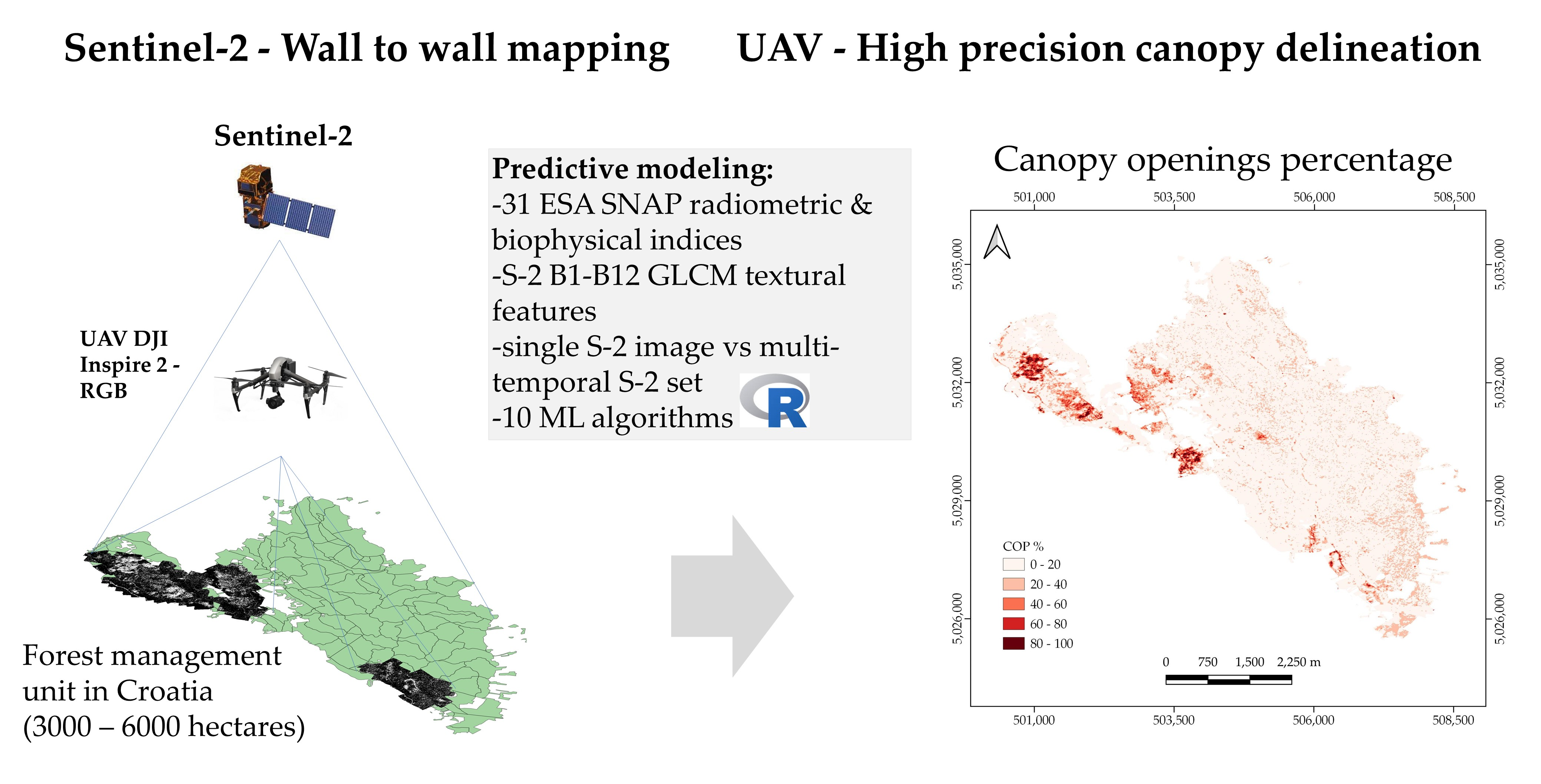
2.1. Study Area

The study area was located in the northeastern, continental part of the Dinaric Alps, a massif in southern and southeastern Europe which stretches for 645 km and separates the continental area of the Balkan Peninsula from the Adriatic Sea. The exact location (Figure 1) was near the town of Vrbovsko, Gorski Kotar region, Croatia (45.4282 latitude and 15.0714 longitude). The research covered the Litorić forest managerial unit (FMU), with an area of 3181.82 hectares, which administratively belongs to the Vrbovsko Forest Office, Forest District Delnice, as an integral part of the state-owned forests managed by the Croatian Forests state company. The FMU Litorić is located at an altitude range of 400 to 900 m and it has 91 compartments. The total wood stock is 965,636 m3 (313 m3/ha), and the total annual increment is 202,015 m3 (6.5 m3/ha). FMU Litorić consists of 35.45% common beech with 342,297 m3 of wood stock and 50.11% common fir with stocks of 483,894 m3. In terms of other species, there are also 8.78% mountain maple, 2.88% spruce, and other hardwoods. According to vegetation typology, the research area is part of a very broad range of European mountain beech forests, a subgroup of Illyrian mountainous beech forests [38] of the Dinaric Alps, where the common beech occurs in combination with the common fir and forms special mixed vegetation forests with high biodiversity and economic value. The lithological base is predominantly composed of limestone and dolomite with associated brown soils.
From the perspective of the prevailing end-users in the area, forest managers in the past decade have mostly been concerned with increases in biotic and abiotic damage. Forests in FMU have been influenced by a prolonged outbreak of spruce bark beetle (Pityokteines curvidens), which causes a weakening of the vitality of trees and forest stands with the occurrence of occasional individual and group dieback of trees. Additionally, most likely as a consequence of climate change, very fierce storms with strong winds have appeared in the last few years causing windbreaks and windthrows. The storm that took place at the beginning of November 2017, followed by a few strong wind events in 2018, had a particularly strong impact in terms of the spatial extent of forest damage. During these incidents, mostly fir trees were damaged due to the resistance provided by their canopy, while beech trees were damaged to a much lesser extent. Considering that classical terrestrial methods of observation could not accurately determine the spatial effect of wind damage, subsequent log hauling, and surface remediation for the scale of the whole FMU, the COP estimation method was implemented by combined remote sensing means and the methodology presented in this study.

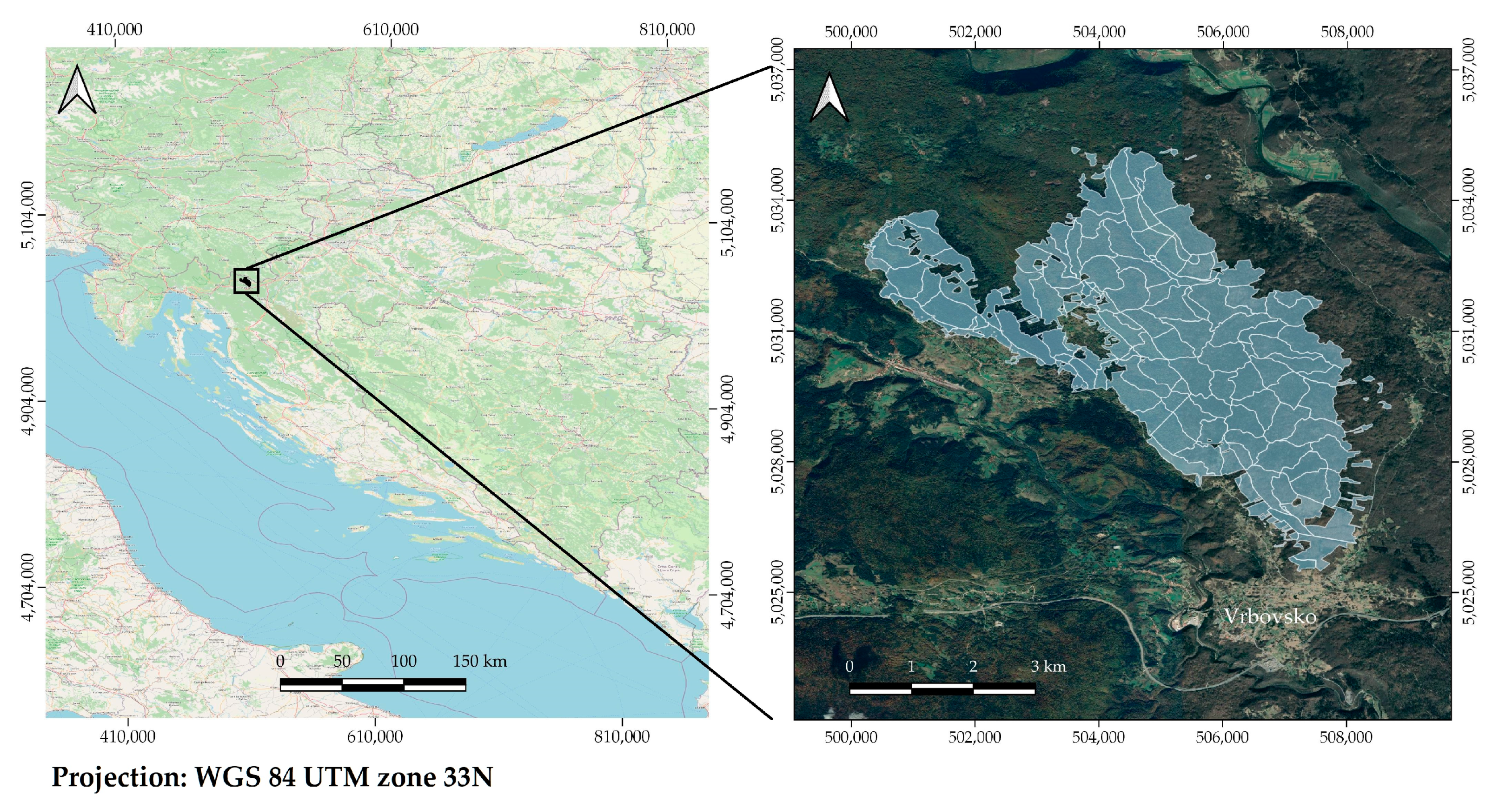
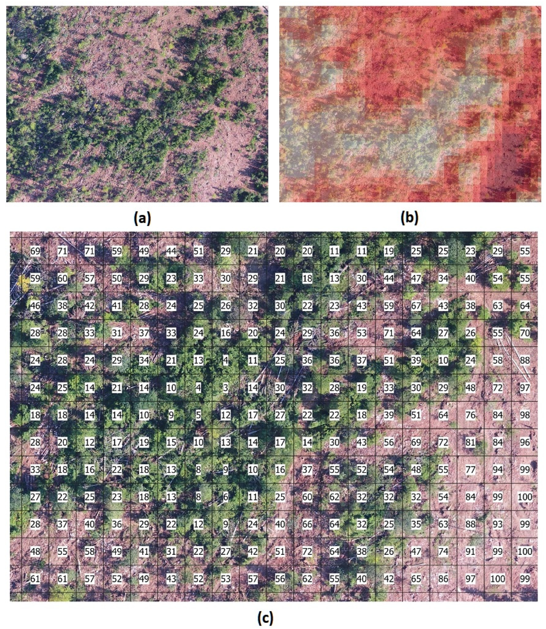
2.2. UAV Survey of the Training and the Testing Area

A detailed survey of the parts of FMU Litorić using UAV was performed at the end of July 2018. The exact time of the survey, the end of July 2018, was selected due to the requirements of the forestry service. Since forest restoration activities at that time were carried out over the entire FMU (logging of remaining fallen trees after windthrows during the winter period and afforestation of the clearings), the interest of the forestry service was focused on obtaining information on the spatial distribution of gaps throughout the FMU to perform the aforementioned silvicultural activities. For this purpose, a UAV survey was first performed at two independent locations, used in this study, where the occurrence of larger windthrows was detected. No particular sampling strategy or design was taken into account when selecting these two sites, with only some preliminary knowledge about forest gap occurrence. After that, Sentinel 2 imagery was preliminarily used, which led to the idea of developing a new methodological approach that would combine both sensing methods, which is presented in this paper. For the survey, a forest service-owned UAV was used with a simple RGB camera, which is otherwise more often used only for visual observation purposes.
One UAV survey area, with a size of 470 hectares, was selected as a training area, and the other, with a size of 310 hectares, was selected as a testing area for selected modeling algorithms (Figure 2). The images in the visible RGB channel were taken using a DJI INSPIRE 2 drone with a ZENMUSE X5S camera with gyroscopic stabilization at a height of 300 m from the ground. All recorded material was transformed in the WGS84 coordinate system. Esri Drone2Map software was used for photo processing and digital orthophoto creation, while cartographic processing was done in the ArcMap 10.6.1. program. The final product presents ortho-rectified high-precision images of the parts of FMU with a spatial grid resolution of 7 cm, through which highly precise canopy boundaries could be delineated and masked out in further processing.

2.3. Satellite Image Processing and Index Extraction

For this study, 4 Sentinel-2 Level 2A (S2_L2A) cloud-free, bottom-of-atmosphere reflectance products were used which consisted of 100 km by 100 km squared ortho-images in UTM/WGS84 projection. Cloud-free imagery, temporarily consistent as much as possible with performed UAV surveys (within an approximately 2-month period), was selected and retrieved from the Copernicus Open Access Hub [38]. Furthermore, all four S2_L2A images had an almost identical time of acquisition and relative orbit position (Table 1). For the purpose of analysis, no additional image enhancement processing of S2_L2A was performed. After the acquisition, due to the differences in pixel resolution, all S2_L2A bands were resampled to a 10 m extent using default resampling processor parameters in the Sentinel Application Platform (SNAP), open-source software provided by the European Space Agency (ESA). Prior to further analysis, the collocation of images was performed, i.e., pixel values of S2_L2A images were resampled into the geographical raster of the master image from 25 July 2018.
The Sentinel 2 multispectral instrument (MSI) has 13 spectral channels in the visible/near-infrared (VNIR) and short-wave infrared spectral range (SWIR) that facilitate the possibility of the construction of a wide range of spectral indices. The development of satellite platforms and sensors over the past decades has also been accompanied by an intensive contrivance of various satellite indices aimed at better discrimination of land surface categories and objects [39]. The fundamental principle of the differentiation of vegetation cover on multispectral images is based on the ratio between the red part of the spectrum that is absorbed by the chlorophyll in the leaves and the infrared part of the spectrum that is reflected by vegetation. Vegetation indices were developed with the intention of clearer quantification of the intensity of vegetation activity with the best possible reduction of accompanying noise. Noise that exists in satellite images and derived indices is usually a consequence of topography, reflection from bare soil, soil color, atmosphere, spectral characteristics of sensors, view, and solar zenith angels [40].
Depending on the approach of noise separation, especially soil line differentiation, vegetation indices are further divided into slope-based, distance-based, and orthogonal [41]. In contrast to a wide range of vegetation indices, soil radiometric indices were primarily developed with the aim of more complete quantification of soil optical properties. Primarily, this refers to the determination of different degrees of soil brightness as a result of viewing geometry, the surface roughness, the organic matter, water contents, and spectral features occurring in the visible domain, i.e., soil color [42]. The more intrinsic insight into the structure and photosynthetic processes of vegetation provide biophysical variables such as Leaf Area Index (LAI), Fraction of Absorbed Photosynthetically Active Radiation (FAPAR), Fraction of Vegetation Cover (FVC), Chlorophyll Content in the Leaf (CAB), and Canopy Water Content (CWC) that present a proxy for the estimation of canopy cover, photosynthetic dynamics, leaf water content can be effectively derived from Sentinel 2 bands [43,44]. A special group of features, developed from digital image analysis, is based on the detection and quantification of gray textures and tones in the images. This can significantly improve the separation of objects and structures in images and is also very suitable for use in various machine learning methods [45].
Considering very heterogeneous surface conditions in the study area of FMU Litorić with various possible spectral feedbacks (areas of undisturbed mixed species canopy, fragments of bare soil surface after logging, open forest gaps with understory shroud of plants and shrubs, occasional groups of sprawled trees, etc.), it was necessarily to use a broader variety of spectral indices. Furthermore, the statistical and machine learning methods can quite successfully isolate the contribution of individual input features on the final predictive outcome. Therefore, various groups of spectral indices such as vegetation indices, soil reflection indices, biophysical variables, and textural properties (gray-level co-occurrence matrix) were used in this study (Table 2). The selection of the applied indices depended on the predefined catalog of indices that can be automatically retrieved through an in-built S-2 index processor in SNAP software. For each of the considered satellite images, (S2_20180725, S2_20180801, S2_20180829, S2_20180928) a total of 155 predictors were calculated: four soil radiometric indices, 21 vegetation radiometric indices, five water radiometric indices, five biophysical indices, and 10 gray-level co-occurrence matrix (GLCM) parameters for each of the S-2 bands (B1-B12), i.e., 120 GLCM layers per S-2 image.

2.4. Integration of Sentinel 2 and UAV Data

One of the fundamental challenges in this research was the integration of satellite S2_L2A and photogrammetric UAV images on the same spatial scale. The S2_L2A multispectral product consists of bands with a spatial resolution of 10 m (band 2, band 3, band 4, and band 8), 20 m (band 5, band 6, band 7, band 11, and band 12), and 60 m (band 1, band 9 and band 10). Before further processing, all bands were rescaled to a 10 m resolution which is a routine procedure in software such as SNAP. All S2_L2A multitemporal products were also collocated on the same spatial grid. The spatial resolution of the UAV images was approximately 7 cm, i.e., 143 times finer than the S2_L2A such that one Sentinel pixel of 10 × 10m contains 20,449 UAV pixels. Although there are available analytical tools that allow rescaling raster images to finer spatial resolution, such processing methods, due to extremely large differences in spatial resolutions of the imagery, were not suitable because they require high-performance computing capabilities and long-term computer processing time. Moreover, the use of R analytical tools in this research, with exceptional capabilities for statistical or machine learning processing, required rearrangement of input spatial data in the standardized R form (a form of matrix or data frame). In that sense, preparation and aggregation of data followed the principles of “tidy” data standardization described by [46], who defines tidy data as follows: each variable forms a column, each observation forms a row, and each type of observational unit forms a table.
Before data aggregation, canopy boundaries were extracted from RGB UAV bands, and a canopy mask layer was created. Acquired aerial imagery was processed similarly to the methodology presented in the research [47]. A generated high-resolution digital orthophoto was used to create various spectral indices that were tested for fast and accurate canopy mask layer creation. In accordance with [48], the best spectral indices were chosen. Although many indices were tested, such as Brightness Index (BI) [49], Redness Index (RI) [50], Color Index (CI) [51], Green Leaf Index (GLI) [52], Normalized Green Red Difference Index (NGRDI) [53], and Visual Atmospheric Resistance Index (VARI) [54], just three of them were selected: NGRDI, VARI, and GLI. Specifically, the mentioned indices mostly distinguish the healthy forest from bare land, windthrows, or canopy openings. The high-resolution UAV-based canopy mask layer was created using the R program language.
The percentage of canopy density for every S2_L2A pixel overlaying the UAV imagery was made by first producing an S2_L2A fishnet grid (regular polygon grid without attributes) with a cell size of 10 × 10 m. Since all S2_L2A images were collocated and resampled, the derived fishnet grid was used on all multitemporal imagery sets. The fishnet grid was then overlapped with regular points i.e., 10 × 10 points (100 points per S2_L2A grid cell). A sampling of the UAV images was performed according to binary outcomes such that the values of the mask layer (forest canopy) were marked as 0 while the areas outside the canopy (forest gaps) were marked as 1. The percentage (COP) for each of the S2_L2A pixels was obtained from the ratio of the sum of 1 (outside the canopy mask) and the total number of points (100) in each grid cell. Then, for each S2_L2A polygon in the fishnet, a centroid was calculated to which the COP value was assigned as a percentage such that each of the pixels on the satellite image was represented with only one point and the corresponding COP value. Further preparation included a random sampling of 10% points on the S2_L2A polygon grid to minimize the effect of spatial correlation between the sampling points on the images. At each selected random centroid or point, sampling of derived satellite indices was performed on multitemporal imagery. After preparation and sampling, all data were compiled into data frames (a training data frame with 4653 observations and 155 predictor variables for a single S2_L2A image and 620 predictors for the entire multitemporal set). The test set consisted of an equal number of input variables and 3596 observations.

2.5. Model Building and Validation

Various statistical and Machine Learning (ML) algorithms of different levels of complexity were examined for the prediction and mapping of the COP. The construction of the models was performed on the training set of observations, retrieved from the selected UAV training area. The performance of different algorithms was examined on the training set across the range of fine-tuning parameters using the 10-fold cross-validation (CV) resampling method and standard metrics that are used in regression analysis: root-mean-square error (RMSE) and the coefficient of determination (R2). The 10-fold cross-validation technique that was used concerning other resampling methods gives the best estimate of the actual RMSE and the most favorable trade-off between the bias and variance of the model [55]. It is also one of the fastest resampling techniques, which is important for the optimization of the computational processing time of the training of some more complex algorithms. All models were also validated on the test set from the physically separate UAV survey area to examine the effect of the spatial extrapolation, using the selected model out of the training area. The procedure of the model construction was repeated twice: the first time using only predictors from the single-date S2_L2A image from 25 July 2018 and the second time using a multitemporal set of the four S2_L2A images, with close dates of acquisition (25 July 2018, 1 August 2018, 29 August 2018, and 28 September 2018). As previously mentioned, the response variable is the COP percentage on the interval quantitative scale (full canopy = 0%; open ground = 100%). All computation was performed in the generic R modeling package Caret, which has the possibility of preprocessing input data, training, testing, and precise adjustment of a large number of statistical and machine learning algorithms [56]. In the R Caret modeling interface, a suitable R package was additionally installed for each of the considered algorithms: stats package for ordinary least squares, pls package for partial least squares, elasticnet package for ridge regression and Elastic Net, nnet package for neural networks, e1071 package for support vector machines, randomForest package for random forest, gbm package for stochastic gradient boosting, xgboost for extreme gradient boosting, and catboost package for CatBoost algorithm. Prior to starting the modeling process, the relationship between COP and individual S2_L2A indices was assessed. Dependency was firstly visually examined on the scatterplots with locally estimated scatterplot smoothing (LOESS) and afterward on simple regression metrics between the COP and the spectral indices. This was performed only on indices from a single S2_L2A 25 July 2018 image which was closest to the date of acquisition of the UAV aero-photo imagery.

2.5.1. Ordinary Least Squares (OLS) Linear Regression

The OLS linear regression method was used as a benchmark model, the results of which served for comparison with other more complex algorithms. Before OLS construction, training data were preprocessed using centering and scaling of predictor variables (zero mean and standard deviation of one). Improvements in the fit by decorrelation and reduction of predictors set using principal component analysis (PCA) and fitting of the PCA components in the OLS model were also examined. OLS, in short, minimizes the sum of squared errors (SSE) between the observed and predicted response, where the parameter estimates that minimize SSE are those with the least bias. OLS is a very attractive technique with regard to the interpretability of the coefficients but has a drawback in that it is sensitive to the collinearity among predictors and is not suitable when the data have a curvature or nonlinear structure.

2.5.2. Partial Least Squares (PLS)

The PLS method is a very suitable technique in the case of high correlation among predictors where OLS is unstable and not appropriate. The principle behind PLS is that it finds the linear combinations of predictors, called components or latent variables, that maximally summarize the variation in the predictor space. Additionally, the determined components have a maximum correlation with the response. PLS has one tuning parameter, i.e., the number of components to retain.

2.5.3. Ridge Regression (RR)

Ridge regression is a linear regularization method suitable where there are issues with collinearity and in cases of overfitting of the data. It belongs to a group of shrinkage methods that add penalties or shrink the parameter estimates which do not contribute significantly to the reduction of the SSE. In the bias–variance trade-off, ridge regression reduces the mean square error by slightly increasing the bias by adding appropriate penalties. The penalty presents a tuning parameter that was optimized by cross-validation during the model training process.

2.5.4. Elastic Net (ENET)

Elastic Net is a linear regularization technique that also effectively deals with highly correlated predictors. It combines two different penalties of the ridge regression and the lasso model. It is an advancement of the ridge regression that also makes possible variable selection that is a characteristic of the lasso model. In the training framework, it is tuned over the various penalty values via cross-validation.

2.5.5. Feed-Forward Neural Networks (NNET)

Neural networks are nonlinear techniques which use hidden variables or hidden units that present linear combinations of the original predictors. Predictors are transformed by a nonlinear function (logistic, sigmoidal) and each unit is related to the outcome. They are characterized by a large number of estimation parameters which are quite uninterpretable. Due to the large number of regression coefficients, neural networks have a tendency of overfitting. The weight decay is a commonly used penalization method that moderates the overfitting problem. In this study, the simplest neural network architecture, a single-layer feed-forward network was used. The tuning parameters used for cross-validation resampling are the number of hidden units and the amount of weight decay.

2.5.6. Support Vector Machine (SVM)

SVM is a nonlinear regression and classification technique that relies on data points (support vectors) above a certain threshold with high residuals. Observations with residuals within the threshold do not contribute to the regression fit, i.e., samples that the model fits well have no effect on the regression equation. This makes SVM insensitive to the outliers, which is very powerful and robust in nature. SVM uses various kernel functions (linear, polynomial, radial basis) that have the ability to model a nonlinear relationship. SVM tuning parameters are the cost parameter that adjusts the complexity of the model (large cost = more flexible model; small cost = “stiffened” model), the size of the threshold for the selection of the vectors, and the kernel parameter.

2.5.7. Random Forest (RF)

Random forest is a tree-based regression and classification ensemble technique that significantly improves the performance of tree-based methods regarding the reduction in variance and bias. It uses a random subset of the predictors at each tree split, which reduces between-tree correlation. The final prediction comprises an average prediction of the models in the ensemble. Models in the ensemble form independent “strong learners” that yield an improvement in error rates. The RF tuning parameter is the number of randomly selected predictors to choose from at each split.

2.5.8. Boosting (GBM, XGBoost, Catboost)

Boosting presents a group of powerful prediction tools, usually outperforming any individual model. The gradient boosting approach relies on the single tree as a base learner and the addition of the “weak learners” which are gradually included in the residuals. The current model is added to the previous model, and the procedure continues for a user-specified number of iterations. When the regression tree is used as the base learner, simple gradient boosting for regression has two tuning parameters: tree depth and the number of iterations. Boosting techniques are currently very popular and are prone to constant improvements. The classical approach presents a Stochastic Gradient Boosting (GBM) algorithm that uses a random sampling scheme. Recently, improved approaches were developed such as XGBoost (Extreme Gradient Boosting) and CatBoost. The advantage of XGBoost over traditional GBM is in its regularization capabilities and more effective tree pruning. However, the new CatBoost model, with improved capabilities of handling categorical variables and overfitting, also shows a significant advantage in the processing speed concerning other boosting methods.

3. Results

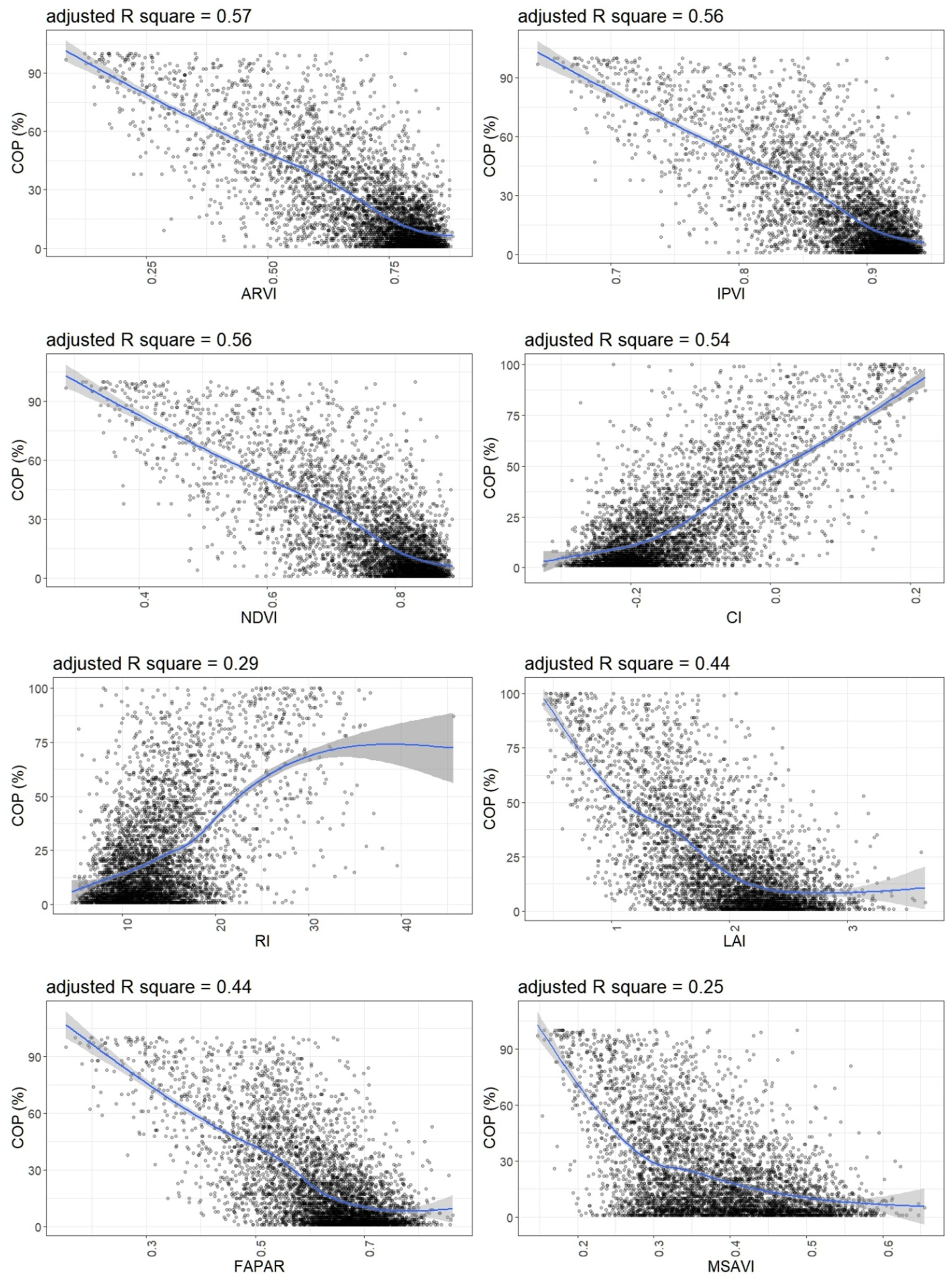
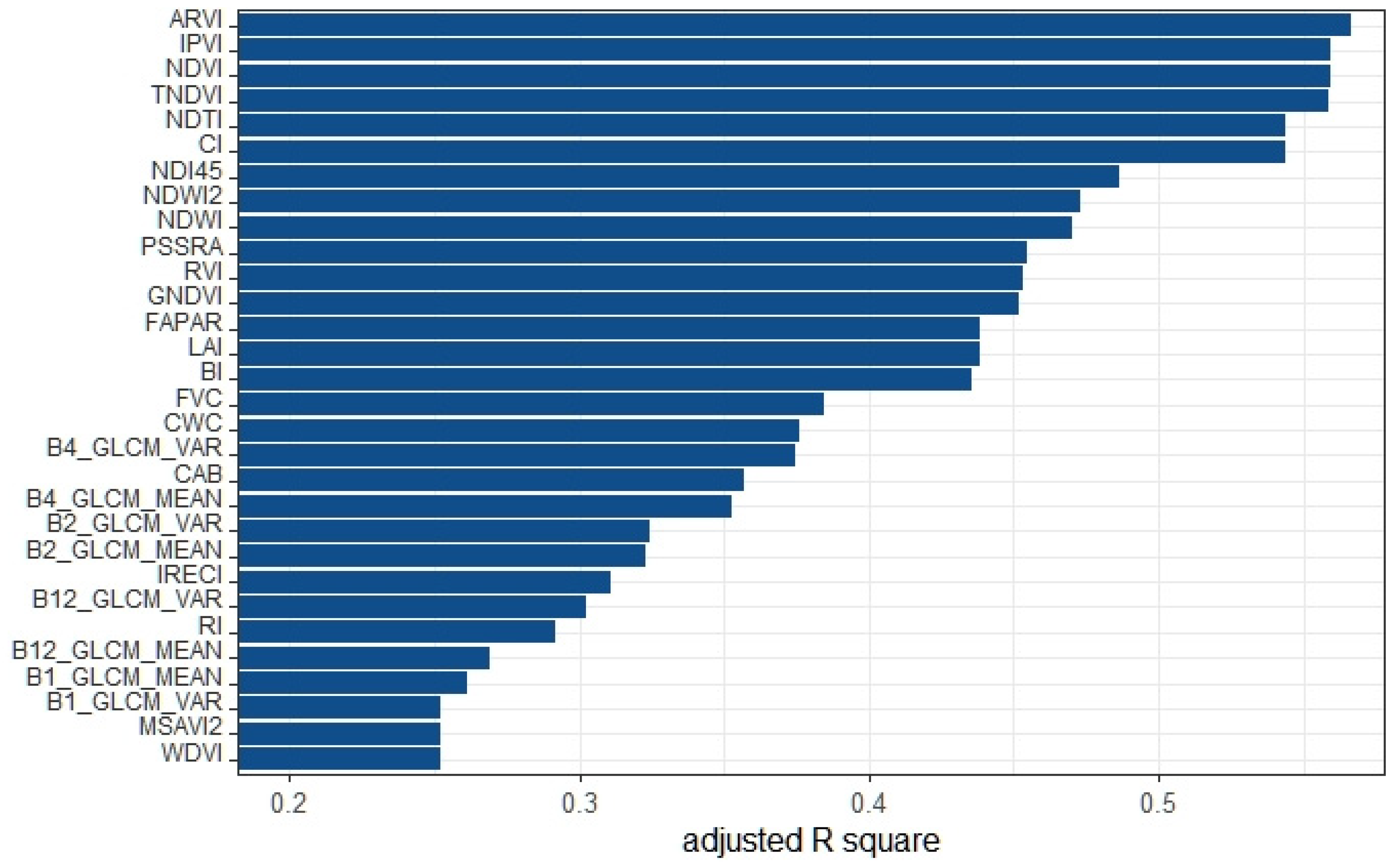
3.1. Relationship of UAV Canopy Openings Percentage (COP) and Individual Sentinel-2 Indices

In Figure 3, which shows scatterplots of selected examples, there is clear evidence of an almost linear negative relationship between COP and the intensity of presented vegetation radiometric indices (NDVI, ARVI, IPVI). Similarly, biophysical indices (FAPAR, LAI) also show a negative relationship in which the nonlinearity between variables is somewhat more pronounced. Soil radiometric indices such as CI and RI show a positive relationship to COP, while the relationship between COP and textural features varies to a certain extent from parameter to parameter.
Figure 4 shows S-2 indices sorted by the coefficient of determination (R2) from the single regression analysis with COP. The best linear relationship with COP (R2 = 0.57) was determined for the ARVI index (Atmospherically Resistant Vegetation Index), followed by the NDVI (Normalized Difference Vegetation Index; R2 = 0.56), and NDVI-derived indices such as IPVI (Infrared Percentage Vegetation Index; R2 = 0.56), TNDVI (Transformed Normalized Difference Vegetation Index; R2 = 0.56), and NDTI (R2 = 0.54). From the so-called soil group of indices, the most significant was CI (Color Index; R2 = 0.54), and, from the water indices, the most significant was NDTI (Normalized Difference Turbidity Index; R2 = 0.54). Derived biophysical indices such as FAPAR (Fraction of Adsorbed Photosynthetically Active Radiation) and LAI (Leaf Area Index) showed a slightly weaker linear association with the dependent variable (both R2 = 0.44). Of the textural features, the most significant relationship was found in the GLCM (gray-level co-occurrence matrix) variance and mean in the red B4 channel (R2 = 0.37, R2 = 0.35).

3.2. Training and Validation of Predictive Models

The results of the model training process of COP and indices from single S-2 image from 25 July 2018 using 10-fold CV are presented in Table 3. It shows the root-mean-square error (RMSE), coefficient of determination (R2), mean absolute error (MAE), and final tuning parameters for each selected model obtained by resampling technique. Compared to simple regression results, the inclusion of multiple predictors from a single S-2 image led to an improvement in prediction, but not to a larger extent. The basic OLS model clearly overfitted the data as is noticeable from the decrease in R2 (from 0.603 to 0.571) when using PCA preprocessing. The addition of other algorithms such as PLS, RR, ENET, NNET, SVM, RF, GBM, XGBoost, and Catboost only slightly improved the prediction results. Complex ensemble models such as XGBoost showed superior results on the training set (R2 = 0.624, RMSE = 15.148, MAE = 11.070). On the other hand, the highly complex NNET algorithm performed below average (R2 = 0.591, RMSE = 15.864, MAE = 11.531).
Model building on the multitemporal S-2 data significantly improved prediction results as is obvious from Table 4. The best results on the training set were provided by the SVM algorithm (R2 = 0.697, RMSE = 13.756, MAE = 9.872) followed by GBM, XGBoost, NNET, RF, CatBoost, and ENET. Simpler algorithms such as PLS and RR performed significantly worse, while the large number of predictors (620) appeared unsuitable for the OLS algorithm (RMSE = 87.413). However, the overall performance of the models of higher complexity showed only small, mostly insignificant improvements.
Validation of the models on the spatially independent test data overall showed much worse results for all the compared models. This is especially evident from the validation results of models based on the single S-2 image, presented in Table 5. The obtained validation metrics, particularly R2, which ranged from 0.380 for SVM to 0.420 for RR and ENET, were significantly lower than the results obtained in the training set. With the addition of the multitemporal S-2 data, there was only a slight improvement in the model performances, as shown in Table 6. The highest R2 value, 0.445, was obtained by the ENET model, followed by other algorithms: CatBoost (R2 = 0.411) and GBM, RF, RR (R2 = 0.440). These results emphasize the problem of spatial extrapolation of the model results or the suitability of the model for prediction outside of the training areas, which is a very common problem in spatial analysis. Furthermore, in the case of extrapolation, the suitability of the simpler, robust, linear regularization algorithms such as ENET and RR was equal to or slightly better than the suitability of the complex ensemble algorithms, which showed better realization only on the training data due to probable overfitting.

3.3. The Importance of Satellite Indices in Prediction

Inferences about the contribution of particular satellite indices in the COP prediction are usually not the main goal in predictive modeling. However, for the purpose of simplifying the building process, particularly retrieval and preprocessing of the huge number of S-2 variables in eventual future similar studies, it is recommended to focus only on the group of the most valuable indices or features that significantly contribute to models. The common drawback of highly flexible modeling techniques such as neural networks, SVM, random forest, and boosting is the lack of interpretability of the model in terms of inferences about the input variables. The important advantage of the R Caret framework is in its capability of quantification of the variable importance in various models. The variable importance is commonly estimated from the reduction in squared error due to each predictor. In ensembles, improvement values for each predictor are averaged across the entire ensemble to yield an overall importance value. The scores of the variable importance estimation for the best-performing models on the multitemporal set in this study are provided in Table 7.
The importance profile of provided scores in Table 7 provides some clues about how models incorporate the data. GBM and XGBoost had a very steep slope of declining scores from top to bottom which is the usual for boosting algorithms. This is due to the fact that trees from boosting are dependent on each other; they have correlated structures as the method follows by the gradient. As a result, many of the same predictors were selected across the trees, increasing their contribution to the importance metric. The RF algorithm relies on the decorrelation of trees and the selection of a random number of variables at each tree node; therefore, it has slower decline in scores. What could be distinguished among the models was the order of incorporating indices from the multitemporal S-2 set across the importance profile. ENET (as well as RR) gradually incorporated the most dominant predictors following the chronology of the multi-temporal S-2 set: first incorporating variables from the first S-2 image, then the second and third (with the exception of the RVI from image four). Incorporation of the most dominant variables from the images in chronological order was probably the learning principle of the regularization algorithm. It slid from image to image, repeatedly incorporated the most significant predictors that reduced SSE, and shrunk or penalized the others. What is also evident is that the ENET model relied only on the first three images in the multitemporal set, and the predictive information from the last set was probably redundant for the model construction. The RF algorithm behaved quite oppositely to the ENET algorithm in that it alternately incorporated variables from the first, then fourth and second S-2 images without some discernible pattern.
Given the spectral indices used, there were also certain peculiarities amongst the models. In most cases, particular vegetation and soil radiometric indices played a dominant role. From the vegetation indices, the most significant were ARVI, IPVI, NDI45, PSSRA, and MCARI, those of soil radiometric indices were CI and RI, and that of water radiometric indices was NDTI. Of the textural features, only GLCM_variance appeared on channel B1 on the last S-2 set. It is also important to note that boosting techniques (GBM, XGBoost) first discriminated sites according to reflectance from the bare soil (CI index) and then from vegetation, unlike other models that built first on reflectance from the vegetation surface.

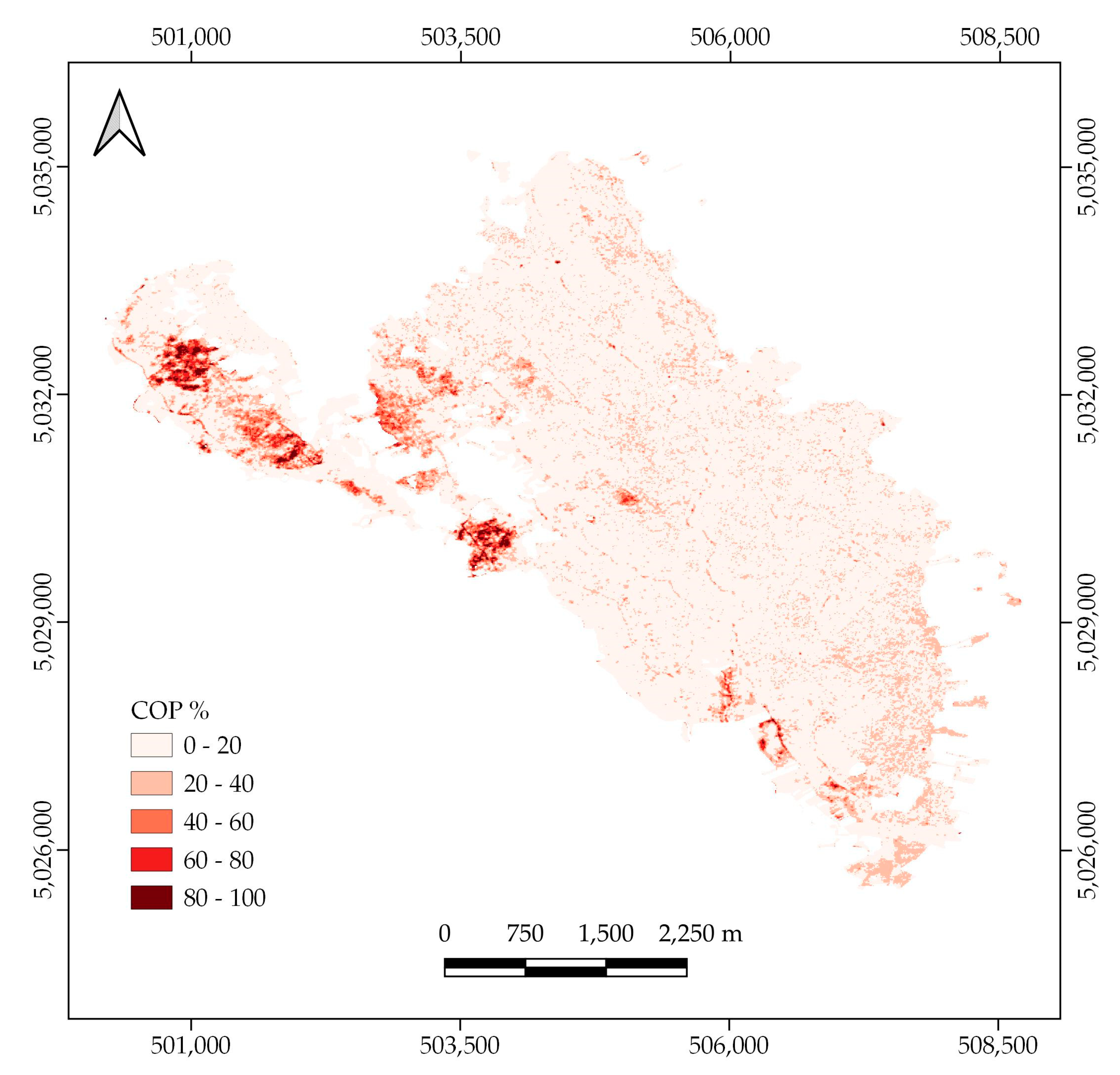
3.4. Final Model Building and COP Map Production

On the basis of the results of training and validation, the ENET algorithm was chosen to create the final model. The main reasons for choosing the ENET model were (I) simplicity of the algorithm, (II) robustness, with best validation results on the test set, (III) one of the shortest computing times amongst all models, and (IV) requirement of the smallest number of S-2 images (three) in the multitemporal set compared to other methods. The final model was produced using all 8222 samples from the training and validation sets, as well as all predictors from the S-2 multitemporal set, 620 in total. The validation metrics of the final ENET model were as follows: RMSE = 14.427, R2 = 0.603, and MAE = 10.821. The model was then used for the prediction of COP over the whole FMU Litorić. Due to the use of regression settings for the prediction of percentages in the interval between 0% and 100%, the final model also contained protruding predictions that were beyond this interval. In such cases, negative values were simply constrained to 0 and values above were constrained to the upper limit of 100. The final result of the whole modeling process, a map of COP percentage for FMU Litorić, is presented in Figure 5. The precision of the produced map can be best perceived by the visual examination of individual details, as presented in Figure 6, which shows a mixed segment with alternating forest cover and clearings.

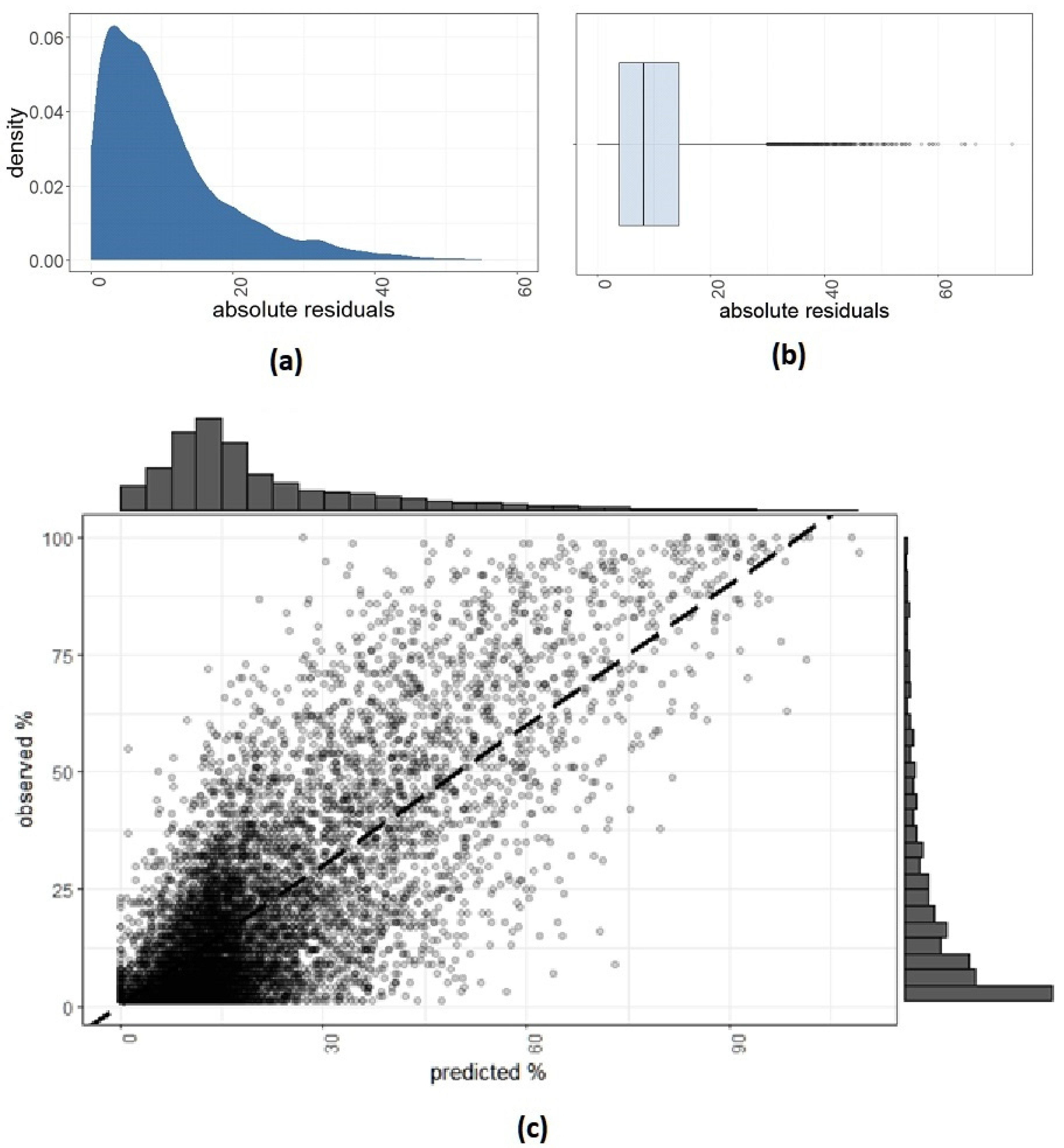
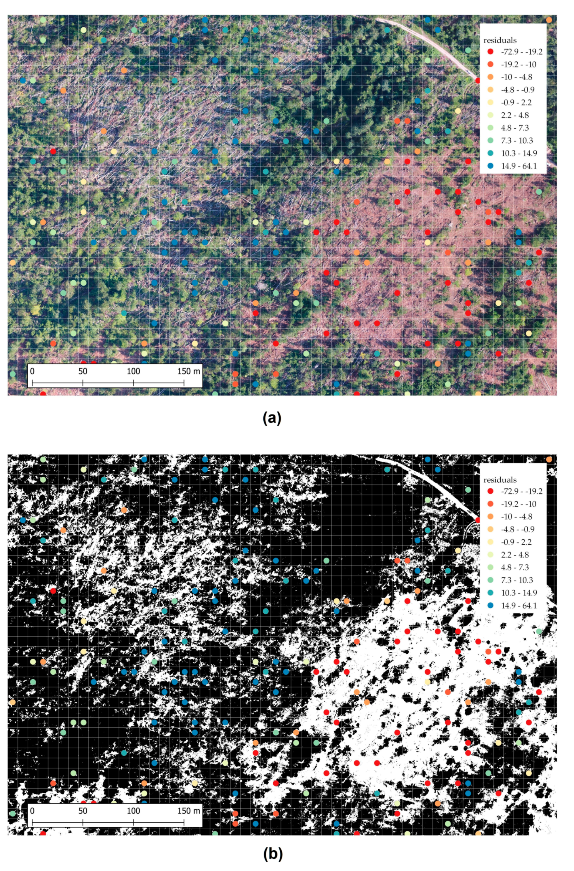
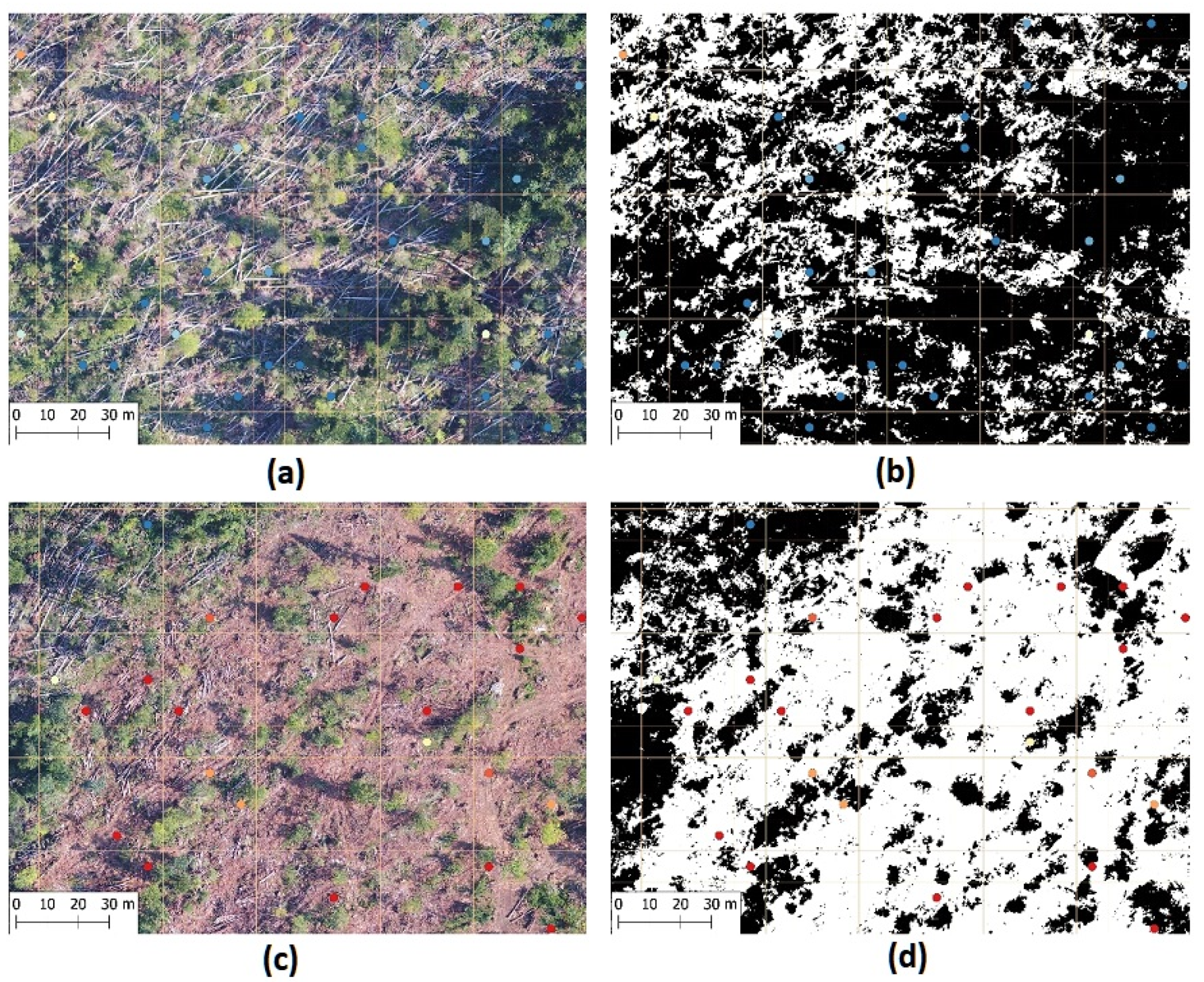
3.5. Analysis of Residuals and Observed Shortcomings of the Model

The relationship of observed vs. predicted values from the final ENET model and the distribution of the residuals are presented in Figure 7.
The model residuals were mainly spatially randomly distributed. In addition, we tried to explain some observed shortcomings of the model with respect to the limited degree of explanation of the variance of response (max R2 of 0.697 in the training set and 0.603 in the final set). This was performed first by gaining insight into spatial patterns of observations with extreme positive and negative residual values and then with further visual examination of the potential reasons for these discrepancies in UAV images. One such case is presented on Figure 8, which shows two larger clearings within the forest on which trees were completely absent. The clearing on the left side of the image contains a group of observations with positive residuals (model over estimation), while the clearing on the right contains a group with negative residuals (model under estimation) Deeper insight is shown in Figure 9.
A deeper insight into the above locations revealed the difference in the surface cover. Specifically, in the image on the left, the fallen trees, as a result of the recent windbreak in the area of FMU Litorić, were noticeable, while, in the image on the right, the trees were completely cleared and the bare soil surface came to expression. Fallen trees, somewhere still with a green canopy, as well as the shadows of the forest edge, were affected by the process of automatic production of the UAV forest mask, which in such cases showed a much lower COP percentage than in reality. The ENET model in such cases provided somewhat realistic COP values that were much higher than the UAV mask. In the figure on the right, the opposite occurred; on bare clearings, the ENET model estimated significantly lower values than in reality, causing negative residuals.
Another case of discrepancy was observed on locations where damaged trees with a higher degree of crown discoloration occurred. These trees that still formed a complete canopy cover were falsely recognized as open areas in the constructed UAV RGB forest mask (Figure 10). This could have caused an unrealistic overestimation of the COP prediction.

4. Discussion

From the presented results of this research, the suitability of the combined method of forest gaps (COP) estimation using UAV and Sentinel 2 images, intended for precise rapid mapping of COP on a large forest management unit scale, was demonstrated. The results of the research show that, with the synergistic effect of two, in many respects, very different Earth observation (EO) systems, we can significantly improve the current practice of monitoring the state and disturbances of forest cover. This approach enables relatively fast and very precise insight into forest canopy over relatively larger areas. There are two particularly important aspects where the significant benefits of using the aforementioned approach could be identified. The first element is related to the improvement of forestry planning and operational activities that could take advantage of the availability of timely and accurate information on the locations and magnitude of forest gaps throughout the FMU. The second element is predominantly contribution in the remote sensing domain, which refers to a proxy way of improvement of the capabilities of Sentinel-2 for very fine gradation of canopy cover at subpixel precision. The effectiveness of the combined use of these two sensors stems from the blending of their comparative advantages and the elimination of their weaknesses. Sentinel-2 is currently one of the most advanced satellite EO systems whose most important features are global coverage, high spectral resolution, and short revisit time, although its spatial resolution is too coarse for the discrimination of canopy openings smaller than 10 m. UAV systems, with ultra-high spatial resolutions and flexibility of manipulation, are currently unsurpassed in capabilities of precise detection of stand coverage, although they are limited in the operational area they can cover. By using the UAV system as ground truth on preselected smaller training and validation areas and Sentinel-2 for wall-to-wall prediction with ML techniques, we extended, in a surrogate fashion, information from the UAV over the whole FMU. Using a simple UAV system with only an RGB camera, which has some limitations in canopy segmentation, has advantages in wide operational applicability. Currently, systems such as DJI drones with RGB cameras are by far the most widespread of all UAV systems, while the processing of such images is far simpler than more complex multispectral, hyperspectral, thermal, and LiDAR images, which greatly facilitates the acquisition of information. As the main purpose of the presented approach is applicability in operational forest management or silvicultural decision-making processes, the method has certain trade-offs that resulted in a somewhat weaker overall prediction accuracy at the expense of the promptness of the required data acquisition and the short time required for the final product manufacturing, which is usually one of the main requirements of end-users in operational forestry for this kind of EO product (e.g., when assessing large-scale calamity caused by windthrows, ice breaks, biotic damages, etc.). The applied approach relies entirely on information from remote sensors in different image resolutions, while it minimizes field work which is in line with current trends of advanced smart forestry technologies.
For the integration of different sensors, UAV and Sentinel-2, the predictive modeling approach was applied, which consisted of feature engineering, the creation of training and validation sets of data, training of various algorithms using resampling techniques, validation of models on the test set, model selection, construction of the final model, and prediction of the new samples. The model building process brought about the improvement in predictive performance on the training set in successive steps; (I) the highest R2 of the single feature (derived satellite index) using simple linear regression was 0.57, (II) the highest R2 using multiple features obtained from the single-date, S-2 image and the best ML algorithm was 0.624, and (III) the highest R2 on the multi-temporal set of four consecutive S-2 images, using the best ML algorithm was 0.697.
From the wider range of satellite indices or features examined in this study, several exhibited superior properties in differentiating the COP gradient and were, therefore, incorporated as the main foundation in the majority of ML models. NDVI (Normalized Difference Vegetation Index), which most often represents the core index for determining variations in the structure of vegetation cover, did not prove to be the primary choice of ML algorithms examined in this research. Instead, as a primary choice, they selected indices closely based on NDVI but with enhanced properties in certain segments. ARVI (Atmospherically Resistant Vegetation Index), as with NDVI, is based on the normalized difference between the near-infrared and red channel, but it corrects the atmospheric effect on the red channel by using the difference in the radiance between the blue and red band. It has a similar dynamic range to NDVI but, on average, is four times less sensitive to atmospheric effects. IPVI (Infrared Percentage Vegetation Index) is functionally equivalent to NDVI with the only difference that it includes infrared and red factors in the NDVI equation which results in simplification of the calculation process. The NDI45 (Normalized Difference Index) algorithm uses the same relations and bands but is more linear and usually less saturated at higher values than the NDVI. In addition to the above indices based on the improved NDVI principle, simple ratio indices that are sensitive to variations in chlorophyll concentrations in canopies were also shown to be the dominant choice for ML algorithms. PSSRa (Pigment-Specific Simple Ratio, or chlorophyll index) consists of a simple ratio of the near-infrared and red bands. It is a narrow-band pigment index that has the strongest and most linear relationship with canopy concentration per unit area of chlorophyll a, chlorophyll b, and carotenoids. MCARI (Modified Chlorophyll Absorption Ratio Index) is the ratio of differences in bands in the visible spectra (red, green, blue), responsive to chlorophyll variation, and ground reflectance. In addition to the mentioned vegetation radiometric indices, a few ML algorithms (GBM and XGBoost), as a first source, used a CI (Color Index) which belongs to the group of soil radiometric indices. CI was primarily developed to differentiate soils in the field, and, in this study, it probably had the best properties to differentiate areas with bare soil within significantly disturbed canopy cover caused by recent windthrows. In most cases, it gave complementary information to the NDVI. RI (Redness Index), as with CI, enables identifying areas with bare soil, which, in the FMU Litorić, have a commonly reddish hue, characteristic for soils developed on hard limestone. Of the other used indices, of greater importance was the NDTI (Normalized Difference Turbidity Index) which belongs to the water radiometric group of indices commonly used for the measurement of water turbidity or water clarity. Since the NDTI algorithm is color-sensitive, with a structure very similar to the CI algorithm, its representation in the models was complementary to the CI and RI indices.
The use of a multitemporal set of S-2 data, compared to information from the single S-2 image, contributed most significantly to an increase in the prediction results compared to all other examined means of prediction improvement. The highest achieved R2 using 10-fold CV on the training set with data from a single S-2 image from 25 July 2018, which was closest to the UAV image acquisition, was 0.624. However, by including variables from the multitemporal set, a significant increase in the explained COP variance from the multitemporal predictors was achieved (R2 of 0.697). On the other hand, the use of a multitemporal set led to an only slight improvement in RMSE (13.756) compared to single-date variables (15.148), which ultimately made a difference of only 1.3% of COP. The advantages of using a multitemporal set of Sentinel 2 images vs. a single image for the discrimination of forest cover are in accordance with recently published results [57,58]. The most likely reason for the enhanced results of the multitemporal set is that, although the S-2 images were obtained within a short time interval (approximately 2 months), they were able to discern certain variations in phenology that are very significant for discriminating small changes in the forest cover structure. According to the results [58], classifications made using multitemporal Sentinel 2 imagery for two contrasting seasons (spring and autumn) were the most accurate, while classifications based on the single-season spring images were the second most accurate. Classifications made using other combinations of seasons and feature types varied but yielded significantly lower accuracy. Incorporation of the Sentinel-2 image from the early spring aspect could most probably improve the COP prediction, but at the risk of loss of up-to-date insight into the current situation of the forest cover, which is often crucial for operational silvicultural decisions.
The addition of ML models with varying degrees of complexity was one of the options in which an improvement in COP prediction was sought. The included ML algorithms on the single temporal S-2 training set with 10-fold CV only partially contributed to improved prediction. Compared to the basic OLS algorithm (RMSE = 15.684; R2 = 0.603), the best XGBoost model (RMSE = 15.148; R2 = 0.624) only slightly improved the prediction results (a decrease in RMSE of 0.536 and an increase in R2 of 0.021). Although they showed a very small improvement of model metrics, a few ML algorithms such as SVM, RF, GBM, XGBoost, and CatBoost showed somewhat better results, whereas some algorithms such as NNET underperformed and others such as PLS, RR, and ENET had similar capabilities to OLS. A significant difference between the algorithms was noticeable on the multitemporal set between the basic OLS model (RMSE = 87.413; R2 = 0.593) and the best SVM model (RMSE = 13.756; R2 = 0.669). It should be noted that the basic OLS algorithm, due to a large number of predictors, exhibited a problem with convergence and instability (high RMSE) and, therefore, was unsuitable for the multitemporal set.
One of the observed shortcomings of the method is that it was less suitable for extrapolation of COP outside the training area, i.e., lower prediction capabilities for COP mapping of the entire FMU area. This was obvious from the obtained metric from the spatially remote validation dataset. The accuracy achieved on the test set was significantly lower than the accuracy obtained using 10-fold CV resampling on the training set. The best obtained RMSE and R2 on a single S-2 image were 15.09 and 0.42, while those on the multitemporal set were 14.900 and 0.445, respectively, significantly worse than the 10-fold CV from the training data. Furthermore, more complex algorithms that were somewhat superior on the training set did not validate their advantages on the independent set. The benefit of using more complex ML algorithms is that they allow better adjustment to local conditions, while this advantage is lost in cases of extrapolation to new conditions out of the training area. In other words, complex ML algorithms generally overfitted the local condition, while, outside the training area, they were comparable to simpler algorithms with greater robustness and generalization ability. These results indicate the inadequate sampling design of the ground-truth UAV data acquisition used for model creation and mapping of the whole FMU area in this study (the sampling design of UAV locations was not considered preliminary). Poorer generalization capabilities of the model could be remedied by the acquisition of UAV ground-truth images from a larger number of smaller training areas across the FMU to incorporate the variety of conditions (stratified random sampling). The ML model constructed in this way, in addition to encompassing a wider range of diversity, would be used primarily for interpolation between the UAV survey locations rather than extrapolation as was the case in this study. Moreover, the improved sampling design will enable much better performance of more complex ML models (RF and boosting) which are superb for the representation of conditions that are not beyond the range of data used for learning.
Precise and reliable delineation of the crown edge on UAV images presented one of the most important factors affecting the reliability of the model. The problems observed in this study stemmed from the limited capabilities of UAV images only in the visible RGB channel to accurately delineate the crown projection, which was then used as reference values for COP modeling. According to our knowledge, research on the combined application of Sentinel-2 and UAV in similar, highly heterogeneous forest types such as mixed beech–fir forests has not been conducted so far; thus, a direct comparison of the obtained results is not possible. On the other hand, there are results in which a somewhat similar approach was used but in somewhat different forest conditions. In a similar study evaluating tree canopy cover [44], using combined Sentinel-2, Google Earth imagery, and ML methods, significantly better prediction was achieved (R2 = 82.8%, RMSE = 8.68%) than in our study. However, higher accuracy of the assessment was obtained in the semiarid Mediterranean silvopastoral system (Quercus ilex, Quercus suber) with sparse tree density and very contrasting bare soil with a distinctive color. In such conditions, it was possible to identify more clearly the crown boundary and produce a more accurate canopy mask layer, which were the most likely reasons for better assessment. In conditions of extremely complex canopy structure, as is the case with mixed beech–fir forests, special attention should be paid when creating a canopy mask layer. Using images only from the visible part of the spectrum, relying solely on differences in color between the canopy and ground, is often very unreliable due to noise from shadows at gap edges, groups of fallen trees after windthrows, etc. Discoloration and defoliation of individual, partially damaged trees, which are falsely rejected from the canopy mask using an automatic classification based only on color indices from the visible spectra, also represent an observed problem that probably affected the accuracy of the method.

5. Conclusions

The development of new remote sensing methods such as UAV, as well as new satellite sensors and the increasing amount and availability of high-quality and free-of-charge satellite data, opens up new opportunities for improving decision-making support in operational forest management. Satellite data have so far, through a large number of different examples, shown their distinct advantages for the detection of changes in forests, but most often in large areas and in coarser spatial resolution, where their robust nature comes to the fore. The use of satellite Earth observations to obtain more accurate information of forest structure is most often hampered by the need for field collection of ground-truth information required for better representation of forest characteristics, which is often very slow and costly. The so-called change detection methods that have been used most often to quantify differences caused by anthropogenic or natural changes in the forest structure provide only proxy, indirect representations inherited from the properties of the used satellite index. On the other hand, the development of unmanned aerial vehicles and their applications in forest photogrammetry have made it possible to obtain very precise, near-real-time information on the forest structure in a very cost-efficient way. The high precision of photogrammetric UAV methods, due to the immense amount of information, and the limited flying range simultaneously represent constraints in the use of this method over larger areas.
Sentinel-2 MSI, due to its advanced spectral characteristics, frequent revisit time, and free-of-charge data availability, represents a highly usable system for various forestry applications. A prerequisite for more efficient use of Sentinel-2 in operational forestry, as well as other optical sensors, is the establishment of stochastic relationships between obtained reflectance in the various spectral bands on multispectral images as surrogate information from forests and common measurable stand parameters used in forest management.
In this study, we demonstrated the effectiveness but also emphasized detected weaknesses of the combined approach to assessment of one of the basic silvicultural parameters such as canopy openings percentage (inverse of the canopy density percentage) using a series of Sentinel-2 imagery and simple UAV RGB images. With the combined approach, the existing limitations of each sensor were annulled: the coarser spatial resolution of Sentinel 2 and the limited flying range of UAV. UAV imagery was used for precise representation of the canopy cover, and Sentinel-2 was used as a scaling platform for transferring information from UAV to a wider spatial extent, while the connection was established using an adequate ML algorithm. A fairly reliable estimate was obtained using a series of four consecutive Sentinel-2 images collected over a period of just over 2 months, which overlapped in time with the UAV recording. Using only one Sentinel-2 image to compare with UAV gave much poorer results. Additionally, for extrapolation of information over the whole FMU, slightly better final results were obtained by using a simpler and more robust linear regularization algorithm such as Elastic Net rather than other more complex and robust ML methods (random forest, boosting, support vector machines, neural networks).
Given its applicability in forestry, the method can be used for operational applications in support of silvicultural planning and decision-making on an annual basis or any time when there is a need from users for up-to-date information of the state of the forest canopy, such as in case of identified disturbances (windthrows, ice breakage), as well as for control of silvicultural or other activities (forest clearings, illegal loggings, etc.). Although the approach was demonstrated in very heterogeneous conditions such as those prevalent in the uneven-aged mixed beech–fir forest, it is possible to extend it to various other forest types and environmental conditions. Furthermore, this approach is suitable for combining Sentinel-2 with other structural and functional parameters of stands that can be obtained directly from UAV sensors (LiDAR, multispectral, hyperspectral) in which there is a stochastic relationship with Sentinel-2 images.

Author Contributions

Conceptualization, I.P. and D.K.; methodology, I.P. and D.K.; validation, I.P. and D.K.; formal analysis, I.P., M.G., and A.N.; writing—original draft preparation, I.P., M.G., and A.N.; writing—review and editing, I.P., M.G., and D.K. All authors have read and agreed to the published version of the manuscript.

Funding

This research received no external funding.

Acknowledgments

This research was undertaken as an additional activity within the Horizon 2020 project “My Sustainable Forest—Earth Observation services for silviculture”.

Conflicts of Interest

The authors declare no conflict of interest.

References

  1. Čater, M.; Diaci, J.; Roženbergar, D. Gap size and position influence variable response of Fagus sylvatica L. and Abies alba Mill. For. Ecol. Manag. 2014, 325, 128–135. [Google Scholar] [CrossRef]
  2. Dobrowolska, D.; Veblen, T.T. Treefall-gap structure and regeneration in mixed Abies alba stands in central Poland. For. Ecol. Manag. 2008, 255, 3469–3476. [Google Scholar] [CrossRef]
  3. Ugarković, D.; Tikvić, I.; Popić, K.; Malnar, J.; Stankić, I. Microclimate and natural regeneration of forest gaps as a consequence of silver fir (Abies alba Mill.) dieback. J. For. 2018, 5–6, 235–245. [Google Scholar]
  4. Muscolo, A.; Sidari, M.; Mercurio, R. Variations in soil chemical properties and microbial biomass in artificial gaps in silver fir stands. Eur. J. For. Res. 2007, 126, 59–65. [Google Scholar] [CrossRef]
  5. Muscolo, A.; Sidari, M.; Bagnato, S.; Mallamaci, C.; Mercurio, R. Gap size effects on above and below-ground processes in a silver fir stand. Eur. J. For. Res. 2010, 129, 355–365. [Google Scholar] [CrossRef]
  6. Albanesi, E.; Gugliotta, O.I.; Mercurio, I.; Mercurio, R. Effects of gap size and within-gap position on seedlings establishment in silver fir stands. Forest 2005, 2, 358–366. [Google Scholar] [CrossRef]
  7. Nagel, T.A.; Svoboda, M. Gap disturbance regime in an old-growth Fagus-Abies forest in the Dinaric Mountains, Bosnia-Hercegovina. Can. J. For. Res. 2008, 38, 2728–2737. [Google Scholar] [CrossRef] [Green Version]
  8. Nagel, T.A.; Svoboda, M.; Diaci, J. Regeneration patterns after intermediate wind disturbance in an old-growth Fagus-Abies forest in Southeastern Slovenia. For. Ecol. Manag. 2006, 226, 268–278. [Google Scholar] [CrossRef]
  9. Diaci, J.; Pisek, R.; Boncina, A. Regeneration in experimental gaps of subalpine Picea abies forest in Slovenian Alps. Eur. J. For. Res. 2005, 124, 29–36. [Google Scholar] [CrossRef]
  10. Malcolm, D.C.; Mason, W.I.; Clarke, G.C. The transformation of conifer forests in Britain—Regeneration, gap size and silvicultural systems. For. Ecol. Manag. 2001, 151, 7–23. [Google Scholar] [CrossRef]
  11. Navarro-Cerrillo, R.M.; Camarero, J.J.; Menzanedo, R.D.; Sánchez-Cuesta, R.; Quintanilla, J.L.; Sánchez, S. Regeneration of Abies pinsapo within gaps created by Heterobasidion annosuminduced tree mortality in southern Spain. iForest 2014, 7, 209–215. [Google Scholar] [CrossRef] [Green Version]
  12. Vilhar, U.; Roženbergar, D.; Simončić, P.; Diaci, J. Variation in irradiance, soil features and regeneration patterns in experimental forest canopy gaps. Ann. For. Sci. 2015, 72, 253–266. [Google Scholar] [CrossRef] [Green Version]
  13. Streit, K.; Wunder, K.; Brang, P. Slit-shaped gaps are a successful silvicultural technique to promote Picea abies regeneration in mountain forests of the Swiss Alps. For. Ecol. Manag. 2009, 257, 1902–1909. [Google Scholar] [CrossRef]
  14. Thurnher, C.; Klopf, M.; Hasenauer, H. Forest in Transition: A Harvesting Model for Uneven-aged Mixed Species Forest in Austria. Forestry 2011, 84, 517–526. [Google Scholar] [CrossRef]
  15. Abdollahnejad, A.; Panagiotidis, D.; Surový, P. Forest canopy density assessment using different approaches—Review. J. For. Sci. 2017, 63, 106–115. [Google Scholar] [CrossRef]
  16. Paletto, A.; Tosi, V. Forest canopy cover and canopy closure: Comparison of assessment techniques. Eur. J. For. Res. 2009, 128, 265–272. [Google Scholar] [CrossRef]
  17. Karhonen, L.; Karhonen, K.T.; Rautiainen, M.; Stenberg, P. Estimation of forest canopy cover: A Comparison of Field Measurement Techniques. Silva Fenn. 2006, 40, 577–588. [Google Scholar] [CrossRef] [Green Version]
  18. Arumäe, T.; Lang, M. Estimation of canopy cover in dense mixed-species forests using airborne lidar data. Eur. J. Remote Sens. 2017, 51, 132–141. [Google Scholar] [CrossRef]
  19. Wu, X.; Shen, X.; Cao, L.; Wang, G.; Cao, F. Assessment of Individual Tree Detection and Canopy Cover Estimation using Unmanned Aerial Vehicle based Light Detection and Ranging (UAV-LiDAR) Data in Planted Forests. Remote Sens. 2019, 11, 908. [Google Scholar] [CrossRef] [Green Version]
  20. Deutcher, J.; Granica, K.; Steinegger, M.; Hirschmugl, M.; Perko, R.; Schardt, M. Updating Lidar-derived Crown Cover Density Products with Sentinel-2. IGARSS 2017, 2867–2870. [Google Scholar] [CrossRef]
  21. Karna, K.Y.; Penman, T.D.; Aponte, C.; Bennett, L.T. Assessing Legacy Effects of Wildfires on the Crown Structure of Fire-Tolerant Eucalypt Trees Using Airborne LiDAR Data. Remote Sens. 2019, 11, 2433. [Google Scholar] [CrossRef] [Green Version]
  22. Huang, C.; Yang, L.; Wylie, B.; Homer, C. A strategy for estimating tree canopy density using Landsat 7 ETM+ and high resolution images over large areas. In Proceedings of the Third International Conference on Geospatial Information in Agriculture and Forestry, Denver, CO, USA, 5–7 November 2001. [Google Scholar]
  23. Mon, M.S.; Mizoue, N.; Htun, N.Z.; Kajisa, T.; Yoshida, S. Estimating forest canopy density of tropical mixed deciduous vegetation using Landsat data; a comparison of three classification approaches. Int. J. Remote Sens. 2012, 33, 1042–1057. [Google Scholar] [CrossRef]
  24. Baynes, J. Assessing forest canopy density in a highly variable landscape using Landsat data and FCD Mapper software. Aust. For. 2004, 67, 247–253. [Google Scholar] [CrossRef]
  25. Joshi, C.; De Leeuw, J.; Skidmore, A.K.; van Duren, I.C.; van Oosten, H. Remote sensed estimation of forest canopy density: A comparison of the performance of four methods. Int. J. Appl. Earth Obs. Geoinf. 2006, 8, 84–95. [Google Scholar] [CrossRef]
  26. Korhonen, L.; Hadi Packalen, P.; Rautiainen, M. Comparison of Sentinel-2 and Landsat 8 in the estimation of boreal forest canopy cover and leaf area index. Remote Sens. Environ. 2017, 195, 259–274. [Google Scholar] [CrossRef]
  27. Mulatu, K.A.; Decuyper, M.; Brede, B.; Kooistra, L.; Reiche, J.; Mora, B.; Herold, M. Linking terrestrial LiDAR scanner and conventional forest structure measurements with multi-modal satellite data. Forests 2019, 10, 291. [Google Scholar] [CrossRef] [Green Version]
  28. Revill, A.; Florence, A.; MacArthur, A.; Hoad, S.; Rees, R.; Williams, M. Quantifying uncertainity and bridging the scaling ga pin the retrieval of leaf area indeks by coupling Sentinel-2 and UAV observations. Remote Sens. 2020, 12, 1843. [Google Scholar] [CrossRef]
  29. Copernicus Land Monitoring Service. Available online: https://land.copernicus.eu/ (accessed on 15 August 2020).
  30. Sentinel 2 User Handbook; Rev 2; European Space Agency: Paris, France, 2015; p. 64. Available online: https://sentinel.esa.int/documents/247904/685211/Sentinel-2_User_Handbook (accessed on 18 August 2020).
  31. Lima, T.A.; Beuchle, R.; Langner, A.; Grecchi, R.C.; Griess, V.C.; Achard, F. Comparing Sentinel-2 MSI and Landsat 8 OLI imagery for monitoring selective logging in the Brazilian Amazon. Remote Sens. 2019, 11, 961. [Google Scholar] [CrossRef] [Green Version]
  32. Masiliūnas, D. Evaluating the potential of Sentinel-2 and Landsat image time series for detecting selective logging in the Amazon. In Geo-Information Science and Remote Sensing; Thesis Report GIRS-2017-27; Wageningen University and Research Centre: Wageningen, The Netherlands, 2017; p. 54. [Google Scholar]
  33. Barton, I.; Király, G.; Czimber, K.; Hollaus, M.; Pfeifer, N. Treefall gap mapping using Sentinel-2 images. Forests 2017, 8, 426. [Google Scholar] [CrossRef] [Green Version]
  34. Šimić Milas, A.; Rupasinghe, P.; Balenović, I.; Grosevski, P. Assessment of Forest Damage in Croatia using Landsat-8 OLI Images. SEEFOR 2015, 6, 159–169. [Google Scholar] [CrossRef] [Green Version]
  35. Navarro, J.A.; Algeet, N.; Fernández-Landa, A.; Esteban, J.; Rodríguez-Noriega, P.; Guillén-Climent, M.L. Integration of UAV, Sentinel-1, and Sentinel-2 Data for Mangrove Plantation Aboveground Biomass Monitoring in Senegal. Remote Sens. 2019, 11, 77. [Google Scholar] [CrossRef] [Green Version]
  36. Pla, M.; Bota, G.; Duane, A.; Balagué, J.; Curcó, A.; Gutiérrez, R.; Brotons, L. Calibrating Sentinel-2 imagery with multispectral UAV derived information to quantify damages in Mediterranean rice crops caused by Western Swamphen (Porphyrio porphyrio). Drones 2019, 3, 45. [Google Scholar] [CrossRef] [Green Version]
  37. Castro, C.C.; Gómez, J.A.D.; Martin, J.D.; Sánchez, B.A.H.; Arango, J.L.C.; Tuya, F.A.C.; Diaz-Varela, R. An UAV and satellite multispectral data approach to monitor water quality in small reservoirs. Remote Sens. 2020, 12, 1514. [Google Scholar] [CrossRef]
  38. Copernicus Open Access Hub. Available online: https://scihub.copernicus.eu/ (accessed on 12 February 2020).
  39. Xue, J.; Su, B. Significant Remote Sensing Vegetation Indices: A Review of Developments and Applications. J. Sens. 2017, 17. [Google Scholar] [CrossRef] [Green Version]
  40. Bannari, A.; Morin, D.; Bonn, F. A Review of vegetation indices. Remote Sens. Rev. 1995, 13, 95–120. [Google Scholar] [CrossRef]
  41. Silleos, N.G.; Alexandridis, T.K.; Gitas, I.Z.; Perakis, K. Vegetation Indices: Advances Made in Biomass Estimation and Vegetation Monitoring in the Last 30 Years. Geocarto Int. 2006, 21, 21–28. [Google Scholar] [CrossRef]
  42. Escadafal, R.; Girard, M.C.; Courault, D. Munsell soil color and soil reflectance in the visible spectral bands of landsat MSS and TM data. Remote Sens. Environ. 1989, 27, 37–46. [Google Scholar] [CrossRef]
  43. Djamai, N.; Zhong, D.; Fernandes, R.; Zhou, F. Evaluation of Vegetation Biophysical variables Time Series Derived from Synthetic Sentinel-2 Images. Remote Sens. 2019, 11, 1547. [Google Scholar] [CrossRef] [Green Version]
  44. Godinho, S.; Guiomar, N.; Gil, A. Estimating tree canopy cover percentage in a mediterranean silvopastoral systems using Sentinel-2A imagery and the stochastic gradient boosting algorithm. Int. J. Remote Sens. 2018, 39, 4640–4662. [Google Scholar] [CrossRef]
  45. Haralick, R.; Shanmugam, K.; Dinstein, I. Textural Features for Image Classification. IEEE Trans. Syst. Man Cybern. 1973, 3, 610–621. [Google Scholar] [CrossRef] [Green Version]
  46. Wickham, H. Tidy data. J. Stat. Softw. 2014, 59, 1–23. [Google Scholar] [CrossRef] [Green Version]
  47. Gašparović, M.; Seletković, A.; Berta, A.; Balenović, I. The evaluation of photogrammetry-based DSM from low-cost UAV by LiDAR-based DSM. SEEFOR 2017, 8, 117–125. [Google Scholar] [CrossRef] [Green Version]
  48. Gašparović, M.; Zrinjski, M.; Barković, Đ.; Radočaj, D. An automatic method for weed mapping in oat fields based on UAV imagery. Comput Electron. Agric. 2020, 173, 105385. [Google Scholar] [CrossRef]
  49. Mathieu, R.; Pouget, M.; Cervelle, B.; Escadafal, R. Relationships between satellite-based radiometric indices simulated using laboratory reflectance data and typic soil color of an arid environment. Remote Sens. Environ. 1998, 66, 17–28. [Google Scholar] [CrossRef]
  50. Madeira, J.; Bedidi, A.; Cervelle, B.; Pouget, M.; Flay, N. Visible spectrometric indices of hematite (Hm) and goethite (Gt) content in lateritic soils: The application of a Thematic Mapper (TM) image for soil-mapping in Brasilia, Brazil. Int. J. Remote Sens. 1997, 18, 2835–2852. [Google Scholar] [CrossRef]
  51. Escadafal, R.; Huete, A. Etude des propriétés spectrales des sols arides appliquée à l’amélioration des indices de végétation obtenus par télédétection. In Comptes Rendus de l’Académie des Sciences. Série 2, Mécanique, Physique, Chimie, Sciences de l’univers, Sciences de la Terre; Gauthier-Villars: Paris, France, 1991; Volume 312, pp. 1385–1391. [Google Scholar]
  52. Louhaichi, M.; Borman, M.M.; Johnson, D.E. Spatially located platform and aerial photography for documentation of grazing impacts on wheat. Geocarto Int. 2001, 16, 65–70. [Google Scholar] [CrossRef]
  53. Tucker, C.J. Red and photographic infrared linear combinations for monitoring vegetation. Remote Sens. Environ. 1979, 8, 127–150. [Google Scholar] [CrossRef] [Green Version]
  54. Gitelson, A.A.; Kaufman, Y.J.; Stark, R.; Rundquist, D. Novel algorithms for remote estimation of vegetation fraction. Remote Sens. Environ. 2002, 80, 76–87. [Google Scholar] [CrossRef] [Green Version]
  55. Kuhn, M.; Johnson, K. Applied Predictive Modeling; Springer: New York, NY, USA, 2013; p. 615. [Google Scholar]
  56. The Caret Package. Available online: http://topepo.github.io/caret/index.html (accessed on 18 May 2020).
  57. Wittke, S.; Yu, X.; Karjalainen, M.; Hyyppä, J.; Puttonen, E. Comparison of two-dimensional multitemporal Sentinel-2 data with three dimensional remote sensing data sources for forest inventory parameter estimation over a boreal forest. Int. J. Appl. Earth Obs. Geoinf. 2019, 76, 167–178. [Google Scholar] [CrossRef]
  58. Macintyre, P.; van Niekerk, A.; Mucina, L. Efficacy of multi-season Sentinel-2 imagery for compositional vegetation classification. Int. J. Appl. Earth. Obs. Geoinf. 2020, 85, 101980. [Google Scholar] [CrossRef]
Figure 1. The location of the study area, forest management unit (FMU) “Litorić”.
Remotesensing 12 03925 g001
Figure 2. The locations of training and testing areas.
Remotesensing 12 03925 g002
Figure 3. The relationship between individual predictors and canopy openings percentage (COP) with included local regression line (LOESS).
Remotesensing 12 03925 g003
Figure 4. The adjusted coefficient of determination of the 30 most dominant predictors (indices) using simple linear ordinary least squares (OLS) regression.
Remotesensing 12 03925 g004
Figure 5. The final map of canopy openings percentage for FMU Litorić.
Remotesensing 12 03925 g005
Figure 6. Representation of map precision. (a) Detail of the area obtained using UAV image; (b) the same detail with overlaid COP map including marked areas in red that indicate disturbances in the canopy; (c) precision of the map can be also perceived from the labels that display COP values in percentages across the S-2 polygon grid.
Remotesensing 12 03925 g006
Figure 7. Assessment of the final model residuals. (a) Density plot of absolute residuals of the ENET model; (b) boxplot of absolute residuals (median value = 8.2%); (c) scatterplot of the predicted vs. observed values with distribution histograms.
Remotesensing 12 03925 g007
Figure 8. Representation of two cases of model discrepancies. (a) Contrasting areas of COP overestimation (blue points) and underestimation (red points); (b) the same forest segments with the UAV mask overlay with visible dissimilarity in abundance of open areas marked in white.
Remotesensing 12 03925 g008
Figure 9. Deeper insight into two contrasting areas. (a) An area with fallen trees after a windstorm; (b) comparative UAV mask that overestimates real forest cover; (c) forest clearing with removed logs and noticeable bare ground with distinguishable soil color; (d) comparative UAV mask of the forest clearing with scarce canopy cover.
Remotesensing 12 03925 g009
Figure 10. Example of false canopy gap creation from UAV RGB images over the damaged trees with crown discoloration. (a) UAV image segment of trees with the damaged canopy; (b) related UAV mask with false open spaces presented in white.
Remotesensing 12 03925 g010
Table 1. Details of Sentinel 2 Level 2A products used in this study.
Platform IDYearMonthDayTime of AcquisitionRelative Orbit NumberTile Number Field
S2A201872510:00 a.m.R122T33TVL
S2B20188110:00 a.m.R122T33TVL
S2B201882910:00 a.m.R122T33TVL
S2B201892810:00 a.m.R122T33TVL
Table 2. Derived satellite indices and textural features.
Satellite IndexSpectral BandsSentinel 2 Bands
Soil radiometric indices
BI—Brightness Indexred, greenB4, B3
BI2—The Second Brightness Indexred, green, NIR(near infrared)B4, B3, B8
RI—Redness Index red, greenB4, B3
CI—Color Index red, greenB4, B3
Vegetation radiometric indices
SAVI—Soil-Adjusted Vegetation Indexred, NIRB4, B8
NDVI—Normalized Difference Vegetation Indexred, NIRB4, B8
TSAVI—Transformed Soil-Adjusted Vegetation Indexred, NIRB4, B8
MSAVI—Modified Soil-Adjusted Vegetation Indexred, NIRB4, B8
MSAVI2—The Second Modified Soil-Adjusted Vegetation Indexred, NIRB4, B8
DVI—Difference Vegetation Indexred, NIRB4, B8
RVI—Ratio Vegetation Index red, NIRB4, B8
PVI—Perpendicular Vegetation Indexred, NIRB4, B8
IPVI—Infrared Percentage Vegetation Indexred, NIRB4, B8
WDVI—Weighted Difference Vegetation Indexred, NIRB4, B8
TNDVI—Transformed Normalized Difference Vegetation Indexred, NIRB4, B8
GNDVI—Green Normalized Difference Vegetation Indexgreen, NIRB3, B7
GEMI—Global Environmental Monitoring Index red, NIRB4, B8A
ARVI—Atmospherically Resistant Vegetation Indexred, blue, NIRB4, B2, B8
NDI45—Normalized Difference Indexred, red edgeB4, B5
MTCI—Meris Terrestrial Chlorophyll Indexred, red edge, NIRB4, B5, B6
MCARI—Modified Chlorophyll Absorption Ratio Index red, red edge, greenB4, B5, B3
REIP—Red-Edge Inflection Point Index red, red edge, red edge, NIRB4, B5, B6, B7
S2REP—Red-Edge Position Indexred, red edge, red edge, NIRB4, B5, B6, B7
IRECI—Inverted Red-Edge Chlorophyll Indexred, red edge, red edge, NIRB4, B5, B6, B7
PSSRa—Pigment-Specific Simple Ratio Indexred, NIRB4, B7
Water Radiometric Indices
NDWI—Normalized Difference Water IndexNIR, MIR(mid-infrared)B8, B12
NDWI2—Second Normalized Difference Water Indexgreen, NIRB3, B8
MNDWI—Modified Normalized Difference Water Indexgreen, MIRB3, B12
NDPI—Normalized Difference Pond Index green, MIRB3, B12
NDTI—Normalized Difference Turbidity Index red, greenB4, B3
Biophysical indices
LAI—Leaf Area Index B3, B4, B5, B6, B7, B8a, B11, B12, cos(viewing_zenith), cos(sun_zenith), cos(sun_zenith), cos(relative_azimuth_angle)
FAPAR—Fraction of Absorbed Photosynthetically Active Radiation
FVC—Fraction of Vegetation Cover
CAB—Chlorophyll Content in the Leaf
CWC—Canopy Water Content
Texture (Gray-Level Co-occurrence Matrix, GLCM)
Contrast
Dissimilarity
Homogeneity
Angular Second Moment
Energy
Maximum Probability
Entropy
GLCM Mean
GLCM Variance
GLCM Correlation
Table 3. The results of 10-fold cross-validation (CV) on the training set using a single S-2 image. RMSE, root-mean-square error; MAE, mean absolute error.
10-Fold CV Training Set: Single Sentinel-2 Image
(S2 25 July 2018)
Model RMSER2MAETuning Parameters
Multiple regression (Ordinary Least Squares)—OLS15.6840.60311.366
Multiple regression (Ordinary Least Squares) with PCA pre-processing—OLS with PCA16.3010.57111.909
Partial Least Squares—PLS15.6180.60411.397ncomp = 20
Ridge Regression RR15.6110.60611.305lambda = 0.007142857
Elastic Net—ENET15.6290.60511.314fraction = 1 lambda = 0.01
Model Averaged Neural Network—NNET15.8640.59111.531size = 5 decay = 0.01
Support Vector Machines with Radial Basis Function Kernel—SVM15.3440.62210.784sigma = 0.007735318 C = 2
Random Forest—RF15.3940.61611.374mtry = 10
Stochastic Gradient Boosting—GBM15.3760.61611.206n.trees = 910 interaction.depth = 7
shrinkage = 0.01 n.minobsinnode = 20
Extreme Gradient Boosting—XGBoost15.1480.62411.070nrounds = 550max_depth = 5
eta = 0.025
Catboost—Cboost15.3080.61911.197depth = 8learning_rate = 0.1
leaf_reg = 0.001rsm = 0.95
Table 4. The results of 10-fold CV on the training set using multitemporal S-2 images.
10-Fold CV Training Set: Sentinel 2 Multitemporal
(S2 25 July 2018; S2 1 August 2018; S2 29 August 2018; S2 28 September 2018)
Model RMSER2MAETuning Parameters
Multiple regression (Ordinary Least Squares)—OLS87.4130.59314.458
Partial Least Squares—PLS15.0200.65010.770ncomp = 10
Ridge Regression—RR41.5200.61111.890lambda = 0.1
Elastic Net—ENET14.3600.66910.543fraction = 0.2 lambda = 0.01
Model Averaged Neural Network—NNET14.2300.68010.520size = 11 decay = 0.1
Support Vector Machines with Radial Basis Function Kernel—SVM13.7560.6979.872sigma = 0.001703831 C = 2
Random Forest—RF14.2650.67310.732mtry = 213
Stochastic Gradient Boosting—GBM13.9520.68510.369n.trees = 910 interaction.depth = 7
shrinkage = 0.01 n.minobsinnode = 30
Extreme Gradient Boosting—XGBoost13.9910.68310.348nrounds = 650max_depth = 4
eta = 0.05
Catboost—Cboost14.1950.67610.460depth = 6learning_rate = 0.1
leaf_reg = 0.001rsm = 0.95
Table 5. Model validation on the testing set: a single S-2 image (S2 25 July 2018).
Test Set: Single Sentinel-2 Image (S2 25 July 2018)
Model RMSER2MAE
Multiple regression (Ordinary Least Squares)—OLS15.2640.40611.655
Partial Least Squares—PLS15.2200.41011.450
Ridge Regression—RR15.1100.42011.230
Elastic Net—ENET15.0900.42011.190
Model Averaged Neural Network—NNET15.3600.41011.090
Support Vector Machines with Radial Basis Function Kernel—SVM16.1100.38011.390
Random Forest—RF15.2900.41011.240
Stochastic Gradient Boosting—GBM15.5800.40011.150
Extreme Gradient Boosting—XGBoost15.6450.38711.233
Catboost—Cboost15.4880.40311.171
Table 6. Model validation on the testing set: multitemporal S-2 images.
Test Set—Sentinel-2 Multitemporal
(S2 25 July 2018; S2 1 August 2018; S2 29 August 2018; S2 28 September 2018)
Model RMSER2MAE
Multiple regression (Ordinary Least Squares)—OLS15.2640.40611.655
Partial Least Squares—PLS15.3030.42511.190
Ridge Regression—RR15.3590.44011.140
Elastic Net—ENET14.9990.44510.916
Model Averaged Neural Network—NNET15.8460.40211.447
Support Vector Machines with Radial Basis Function Kernel—SVM16.0200.41011.240
Random Forest—RF14.9000.44010.935
Stochastic Gradient Boosting—GBM14.9400.44010.730
Extreme Gradient Boosting—XGBoost15.1020.42810.874
Catboost—Cboost14.9510.44110.793
Table 7. Variable importance scores for the top 20 satellite indices and related models. The S-2 columns refer to the positioning of the index variable in the multitemporal set (I = 25 July 2018, II = 1 August 2018, III = 29 August 2018, IV = 28 September 2018).
CBoostS-2ScoreGBMS-2ScoreXGBoostS-2Score
IPVII100.00CII100.00CII100.00
NDTII92.57ARVII36.53ARVII33.58
TNDVII75.02NDI45III32.07IPVII33.48
NDI45IV71.79PSSRAI29.16NDI45III19.74
NDI45II54.44NDI45II26.5PSSRAII13.47
NDTIII49.79IPVII22.65NDI45I11.85
NDVIIV41.68NDI45IV16.43NDI45IV11.73
MCARII40.58CIII15.6CIII10.79
ARVII37.70NDI45I15.02IPVIIV5.63
RIII36.04CIIV10.75CIIV5.61
TNDVIIV34.42IPVIIV7.27NDI45I5.50
NDWI2IV32.80ARVIII7.22RIII4.62
CIII32.24RIII7.08MCARIIV4.18
PSSRAI31.53PSSRAII6.04MCARII3.8
NDTIIV30.57CIIII5.99ARVIII3.48
NDTIIII29.08MCARIIV5.65CIIII3.24
GLCM_VAR_B1IV28.21MCARII4.66GLCM_VAR_B1IV2.54
ARVIIV27.97PSSRAII4.61ARVIIV2.46
CIIII27.32NDWI2IV4.08NDWI2IV2.46
NDVII26.11ARVIIV3.64PSSRAII1.78
ENETS-2ScoreRFS-2ScoreSVMS-2Score
ARVII100NDI45IV100ARVII100
TNDVII98.85ARVII80.22TNDVII98.85
IPVII98.85MCARIIV79.45IPVII98.85
NDVII98.85RIII75.48NDVII98.85
RVIIV98.45IPVIIV73RVIIV98.45
RVII98.45PSSRAI71.2RVII98.45
ARVIII97.85MCARII69.72ARVIII97.85
CII97.73CIIV69.61NDTII97.73
NDTII97.73CIII65.47CII97.73
PSSRAI97.46CII65.11PSSRAI97.46
CIII96.73NDVIIV63.8NDTIII96.73
NDTIII96.73NDTII63.28CIII96.73
IPVIII96.4TNDVIIV62.23IPVIII96.4
NDVI II96.4NDTIIV59.98NDVIII96.4
TNDVI II96.4RVIIV59.08TNDVIII96.4
PSSRAII96.28NDTIII57.78PSSRAII96.28
RVIII95.78RVII56.28RVIII95.78
PSSRAIII93.33ARVIIV55.73PSSRAIII93.33
ARVIIII92.24NDVII55.57ARVIIV92.24
NDVIIII91.45TNDVII54.88NDVIIV91.45
Publisher’s Note: MDPI stays neutral with regard to jurisdictional claims in published maps and institutional affiliations.

