Article

A Comparison of UAV and Satellites Multispectral Imagery in Monitoring Onion Crop. An Application in the ‘Cipolla Rossa di Tropea’ (Italy)

1
Dipartimento di Agraria, Università degli Studi Mediterranea di Reggio Calabria, Località Feo di Vito, I-89122 Reggio Calabria, Italy
2
Plant Protection Department, Institute of Agricultural Sciences (ICA), Spanish National Research Council (CSIC), 28006 Madrid, Spain
3
Department of Agricultural, Food, and Environmental Sciences, University of Perugia, 06121 Perugia, Italy
*
Author to whom correspondence should be addressed.
Remote Sens. 2020, 12(20), 3424; https://doi.org/10.3390/rs12203424
Submission received: 21 September 2020 / Revised: 14 October 2020 / Accepted: 16 October 2020 / Published: 18 October 2020
(This article belongs to the Special Issue Digital Agriculture)

Abstract

:
Precision agriculture (PA) is a management strategy that analyzes the spatial and temporal variability of agricultural fields using information and communication technologies with the aim to optimize profitability, sustainability, and protection of agro-ecological services. In the context of PA, this research evaluated the reliability of multispectral (MS) imagery collected at different spatial resolutions by an unmanned aerial vehicle (UAV) and PlanetScope and Sentinel-2 satellite platforms in monitoring onion crops over three different dates. The soil adjusted vegetation index (SAVI) was used for monitoring the vigor of the study field. Next, the vigor maps from the two satellite platforms with those derived from UAV were compared by statistical analysis in order to evaluate the contribution made by each platform for monitoring onion crops. Besides, the two coverage’s classes of the field, bare soil and onions, were spatially identified using geographical object-based image classification (GEOBIA), and their spectral contribution was analyzed comparing the SAVI calculated considering only crop pixels (i.e., SAVI onions) and that calculated considering only bare soil pixels (i.e., SAVI soil) with the SAVI from the three platforms. The results showed that satellite imagery, coherent and correlated with UAV images, could be useful to assess the general conditions of the field while UAV permits to discriminate localized circumscribed areas that the lowest resolution of satellites missed, where there are conditions of inhomogeneity in the field, determined by abiotic or biotic stresses.

Graphical Abstract

1. Introduction

The agricultural sector is one of the areas of application of geographic information systems, remote sensing (RS) methods, and data [1]. The remote platforms and their associated imaging systems are distinguished based on platform altitude, spatial, and temporal resolution. The spatial resolution determines the smallest pixel area that can be identified; thus, as the spatial resolution increases, the pixel area decreases, and the homogeneity of soil or crop characteristics inside the pixel increases [2].
The temporal resolution is essential for the evaluation of time patterns in plant and soil characteristics. However, the availability of RS images from satellite and aerial platforms is limited by cloud cover [3,4,5]. Landsat platforms, among the most used satellites, have spectral resolutions of the order of 30 m in the visible and near-infrared (NIR) and have a temporal resolution close to 17 days [6]. For many precision agriculture (PA) applications, this temporal resolution is not suitable, even considering cloud cover problems that increase the time interval in which images without coverage are available. The same applies to spatial resolution, which may not be suitable for determining variability within the field. The launch of satellites by government space agencies and commercial earth-observing companies has provided a significant improvement in revisiting time and multispectral (MS) detection capability. In this respect, two examples are given by Sentinel-2 and PlanetScope satellites. Sentinel-2 satellites are equipped with sensors capable of exploiting as many as 13 spectral bands ranging from the visible to NIR and short wave infrared region, with spatial resolutions between 10 and 60 meters [7] and a temporal resolution of about 5 days at the European latitudes [8,9]. PlanetScope constellation composed of a large number of small nano-satellites equipped with RGB and NIR camera provides a 3–5 m ground sampling resolution with a one-day revisiting time [10].
While satellite observation has guided many information-based advances in agricultural management and practice [6], critical technological developments and steep rise have affected unmanned aerial vehicles (UAVs) in the last decade, which represent a potential game-changer in PA applications [11]. In comparison with other RS platforms, UAVs are generally more independent of climatic variables.
Being able to provide data with higher temporal and spatial resolution, today represents a significant source of RS imagery in PA [12] considering also that, as highlighted by scholars in PA applications, the knowledge of the within-field spatial variation of edaphic factors and the state of crops constitute an essential prerequisite [13]. Among the sensors mounted on UAVs employed in agriculture, MS cameras are the most common [14].
Thanks to UAVs and high-resolution MS images, the managers and specialists in agriculture can use new tools and have more information to optimize management decisions and formulate precision farming solutions [15]. In particular, this technology can determine the amount of agricultural inputs, including agrochemicals and fertilizers, based on non-invasive monitoring of crop growth status [16].
The ability to better control the use of agrochemicals and fertilizers brings benefits, in addition to the enhanced quality and quantity of production, reducing the environmental risks arising from the excessive use of inputs, increasing the use efficiency, and also reducing them, using variable management practices [17,18].
Many MS UAV cameras, in particular, permit to obtain spectral information in the Red, Red Edge, and NIR band for vegetation applications with a very high spatial resolution [19]. Based on the combination of these three bands, most of the indices (i.e., vegetation indices, VIs) have been developed with the aim to monitor, analyze, and map temporal and spatial variations of vegetation in both field and tree crops [19]. In the framework of PA applications, among the techniques capable of extracting reliable and reusable information, the geographic object-based image classification (GEOBIA) techniques have demonstrated their effectiveness [1].
GEOBIA is a typology of a digital RS image analysis and classification approach that studies geographical entities through the definition and analysis of object-based instead of single pixels [20,21]. Image objects are objects that can be distinguished in the scene. They are formed by groups (or clusters) of neighboring pixels that share a common meaning, such as, for example, in a farm context, pixels that join together to form trees’ canopies of an orchard or crops in a field [22]. In the literature applications of GEOBIA, starting from satellite or UAV data, both herbaceous and tree crops have been concerned [23,24,25,26,27,28,29,30,31,32].
Onion (Allium cepa L.) is a vegetable bulb crop widely cultivated and known to most cultures [33,34]. For economic importance among vegetables, the onion ranks second after the tomato [35,36]. This plant belongs to the family of Amaryllidaceae and is biannual or perennial (depending on the cultivar).
The plant has shallow adventitious fibrous roots [37], which grow, usually in the first 20–25 cm of soil. The umbrella-shaped inflorescence develops from an apical ring meristem and is formed by the aggregation of small single flowers (from 200 to 600).
The bulb has variable shapes (flat to globular to oblong) and colors (red, white, or yellow). The bulb, the edible part, comes from the enlargement of the basal part of the inserted leaves, superimposed on a central cauline axis. The bulb’s thick outer leaves lose moisture and become scaly until harvest, while the inner leaves thicken as the bulb develops [38].
In this framework, this study was aimed at comparing data acquired by fixed-wing UAV and the PlanetScope and Sentinel-2 satellites in onion crop monitoring. RS techniques applied to onion crops could help to monitor the crop growth, guide localized fertilization, phytosanitary treatments, and harvest, and, in general, support PA techniques implementation. To our knowledge, very few studies have dealt with onion crop monitoring using UAV and satellite data in the PA framework [16,23,33,34,39].
Considering the objectives of this research, the study site was located in a very relevant onion production area of Southern Italy. The comparison was performed to achieve the following objectives: a) evaluate the similarities and the informative content of the vegetation index at different spatial resolutions; b) evaluate the contribution made by each platform for monitoring the vegetative status of the onion crop and in guiding fertilization and phytosanitary treatments.
This paper is structured as follows. In Section 2, information about the study site, data acquisition and processing, and data analysis are reported. Section 3 is devoted to presenting and discussing the results. Section 4 deals with conclusions and future research perspectives.

2. Materials and Methods
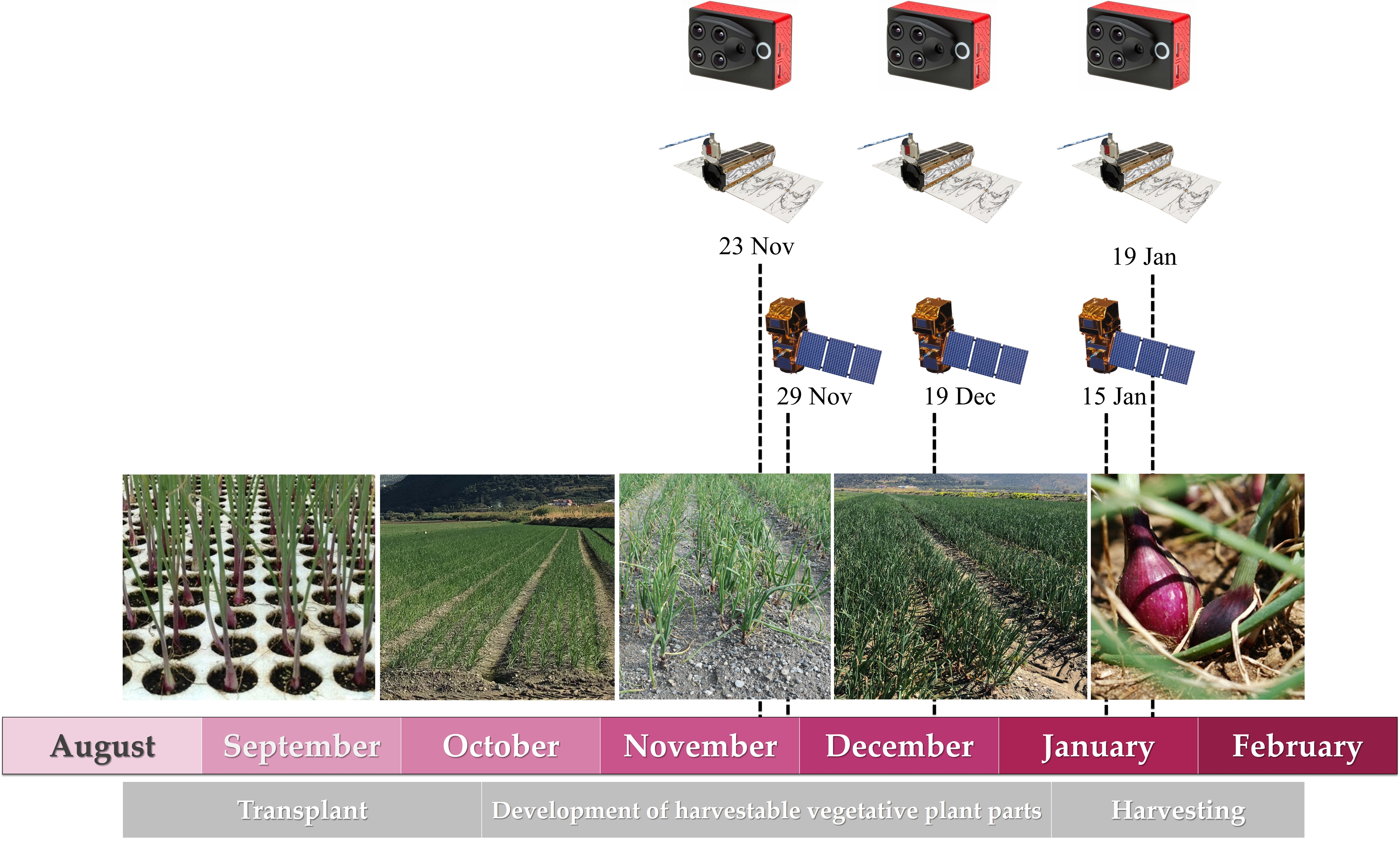
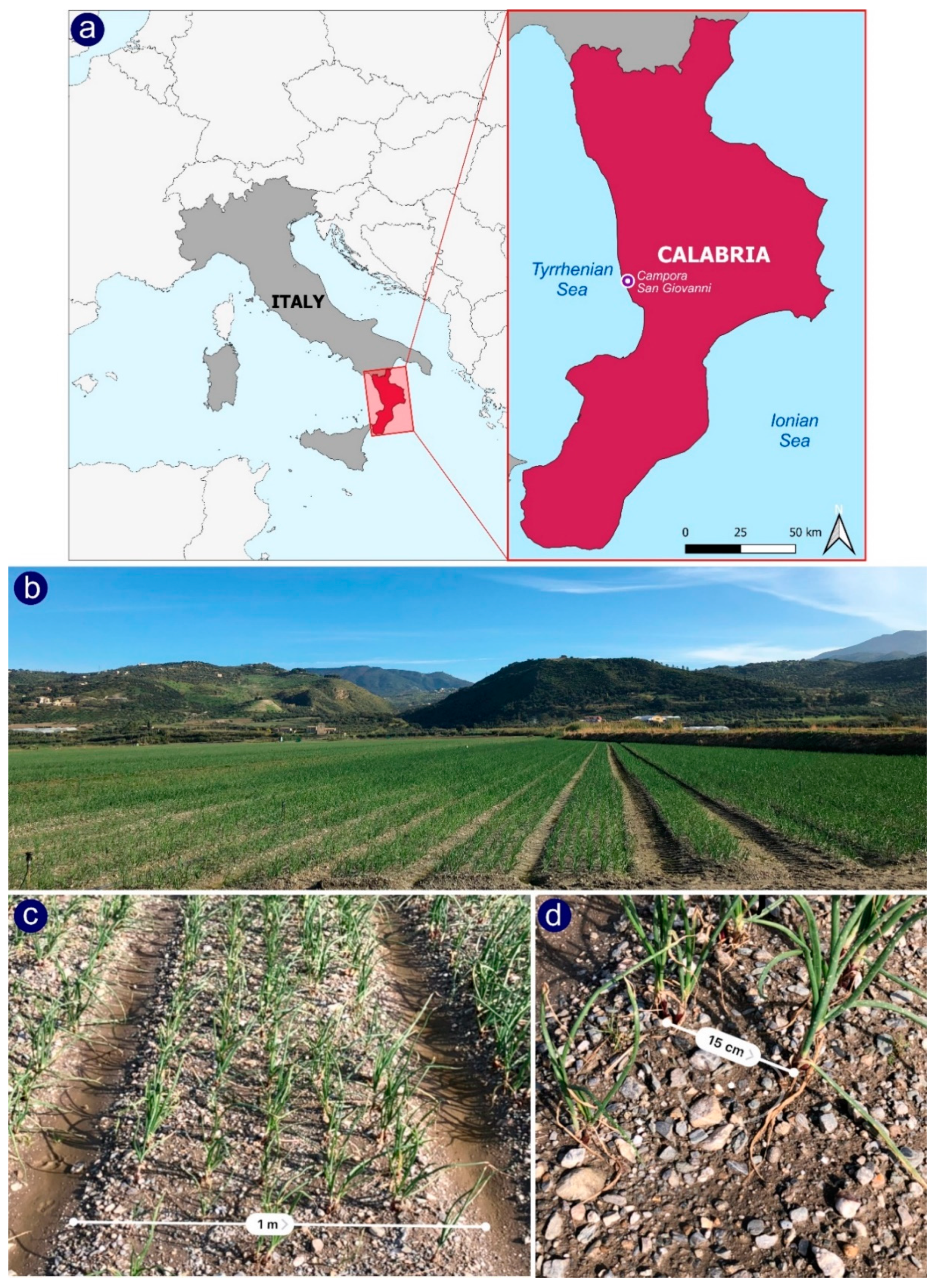
2.1. Study Site

The onion field is located in Campora S. Giovanni, in the municipality of Amantea (Cosenza, Italy, 39°02’ 55’’ N, 16°05’ 59’’ E, 5 m a.s.l) (Figure 1a). The onions produced here are an essential local crop that, as a typical product, plays a crucial role in the economic and rural development of this territory [40]. This particular pink-red colored onion type, since 2008, is labeled with the European Protected Geographical Indication “Cipolla Rossa di Tropea IGP”.
It is well-known worldwide for its sweet flavor and for its high content of nutraceuticals that make it an upcoming “functional food” [41]. These unique characteristics have given the product a reputation at the national level and in markets outside Italy.
The producing farms are organized in a consortium whose cultivated area is over 500 hectares [42]. The study area covers a surface of 4 hectares. The field is crossed by 10 paths, 2.5 m wide, used for the passage of agricultural vehicles necessary for phytosanitary treatments and fertilization. The plants are placed at a distance of 15 cm from each other, on baulature, 1 m wide, as shown in Figure 1b–d.
The transplant took place between mid-August (end of the summer) and mid-September (early autumn). In particular, in a portion of the field, about 0.47 ha, transplantation took place 3 weeks later.

2.2. Platforms and Data Acquisition
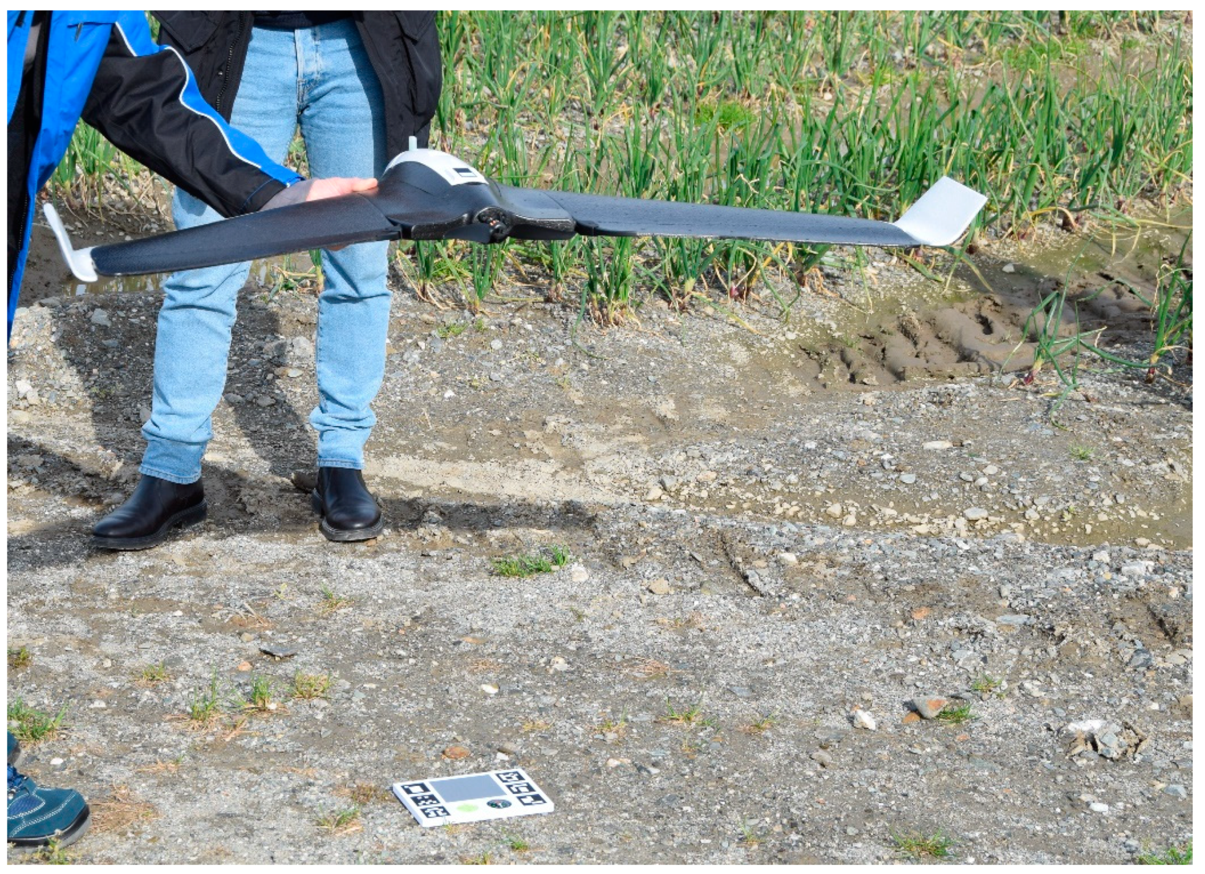
2.2.1. UAV Images

The UAV surveys were carried out between the middle (November) and the end of the cultivation cycle (January). Onion crop was, in this time frame, in the principal stage 4 (development of harvestable vegetative plant parts) (Figure 2) of the BBCH (Biologische Bundesanstalt, Bundessortenamt and Chemical Industry) extended scale [43]. Surveys were carried out at 50 m of flight height using a very light fixed-wing UAV Parrot Disco-Pro AG made with foam and the weight of only 780 g (Figure 3). The UAV was equipped with an MS camera Parrot Sequoia, a light-weight camera employed in several research works related to PA, on herbaceous crops, monitoring wheat [44], maize and poppy crops [45], phenotyping of soybean [46], and on tree crops proving useful in identifying [47] citrus trees [24], mapping irrigation inhomogeneities in an olive grove [48] and the vigor in vineyards [49]. The Parrot Sequoia MS had four different channels, each with 1.2 Mp of resolution: Green (530–570 nm), Red (640–680 nm), Red Edge (730–740 nm), and NIR (770–810 nm). Furthermore, it was also equipped with an RGB composite sensor, an external irradiance sensor with a global navigation satellite system (GNSS), and inertial measurement unit (IMU) modules placed on top of the UAV. The irradiance sensor, which measures the sky down-welling irradiance, was placed on top of the UAV and continuously captured the sky irradiance at the same spectral bands as the MS camera [50,51]. The IMU allowed capturing sensor angle, sun angle, location, and irradiance for every image taken during the flight. This data was mainly used for image calibration. The UAV flights were carried out three times as follows: 23 November 2018, the second on 19 December 2018, and the last on 18 January 2019. The first two dates, as shown in Figure 2, concerned the phase of the crop cycle of the full development of harvestable vegetative plant parts. In this phase, crucial operations were carried out, such as a large part of the fertilization and phytosanitary treatments. Instead, on the last date of monitoring, in January, onions were close to harvesting.
The procedure performed for field surveys was similar to the one shown in Messina et al. [52,53]. In the field, 9 ground control points (GCPs) were placed whose position was geo-referenced using a Leica RTK GNSS with a planimetric accuracy of 0.03 m. In particular, GCPs were made using 50 cm × 50 cm white polypropylene panels and covering two quadrants using black cardboard to locate the point. MS imagery was calibrated using a panel with known reflectance, the Parrot Sequoia calibration target (Figure 3). In particular, photos of the target were taken before and after the flight, and it was assumed that the raw sensor data was transformed into percentage reflectance in combination with the data provided by the solar radiation sensor. All consecutive images were processed via aerial image triangulation with the geo-tagged flight log and the geographic tags through the software Pix4D mapper (Pix4D S.A., Switzerland). Following the recommended Sequoia image correction procedure, corrections were applied to the raw data, generating four single reflectance-calibrated GEOTIFFs.

2.2.2. Satellite Images

Sentinel-2 is managed through the Copernicus Program proposed by the European Union (EU) and the European Space Agency (ESA). The first satellite was launched in 2015 [54]. Sentinel-2 consists of two twin satellites, Sentinel-2A and Sentinel-2B, both operating on a single orbit plane but phased at 180º with a temporal resolution of 5 days with this bi-satellite system [55,56].
The Sentinel-2 data consists of 13 bands in the visible, NIR, and short-wavelength infrared (SWIR) spectral range [55,57] with a spatial resolution of 10 m, 20 m, or 60 m depending on the band. Sentinel-2 images used in this work were the four spectral bands at 10 m spatial resolution in Blue, Green, Red, and NIR spectra, shown in Table 1. Data were downloaded from the Copernicus Open Access Hub [58] in level 2A, which provides the bottom of atmosphere (BOA) reflectance images ortho-rectified in UTM/WGS84 projection.
PlanetScope’s imagery was acquired from the PlanetScope archive [59], which manages the largest satellite constellation consisting of more than 150 satellites orbiting the Earth. PlanetScope satellites follow two different orbital configurations [60]. Some satellites are in International Space Station Orbit (ISS), and they are at a 52° inclination at about 420 km of altitude. Other satellites are in the Sun Synchronous Orbit (SSO) with an altitude of 475 km (at 98° inclination) and have equatorial crossing between 9:30 and 11:30.
These sensors called 3U CubeSats (Table 1), also called “Doves”, have small dimensions (10 cm × 10 cm × 30 cm and a weight of 4 kg) and provide daily sun-synchronous coverage images of the whole Earth landmass [60].
Dove satellites’ CCD array sensor (6600 × 4400 pixels) allows capturing images using three bands RGB or four (in addition, there is NIR) [61]. PlanetScope imagery has a scene footprint of about 24.4 km × 8.1 km and a ground sample distance of 3.7 m.
PlanetScope imagery we used is the Ortho Scene product (Level 3B), i.e., imagery processed to remove distortions caused by terrain. Imagery is radiometrically, sensor, and geometrically corrected [59]. Furthermore, imagery is atmospherically corrected using the 6S radiative transfer model with ancillary data from the moderate resolution imaging spectroradiometer (MODIS) [62].

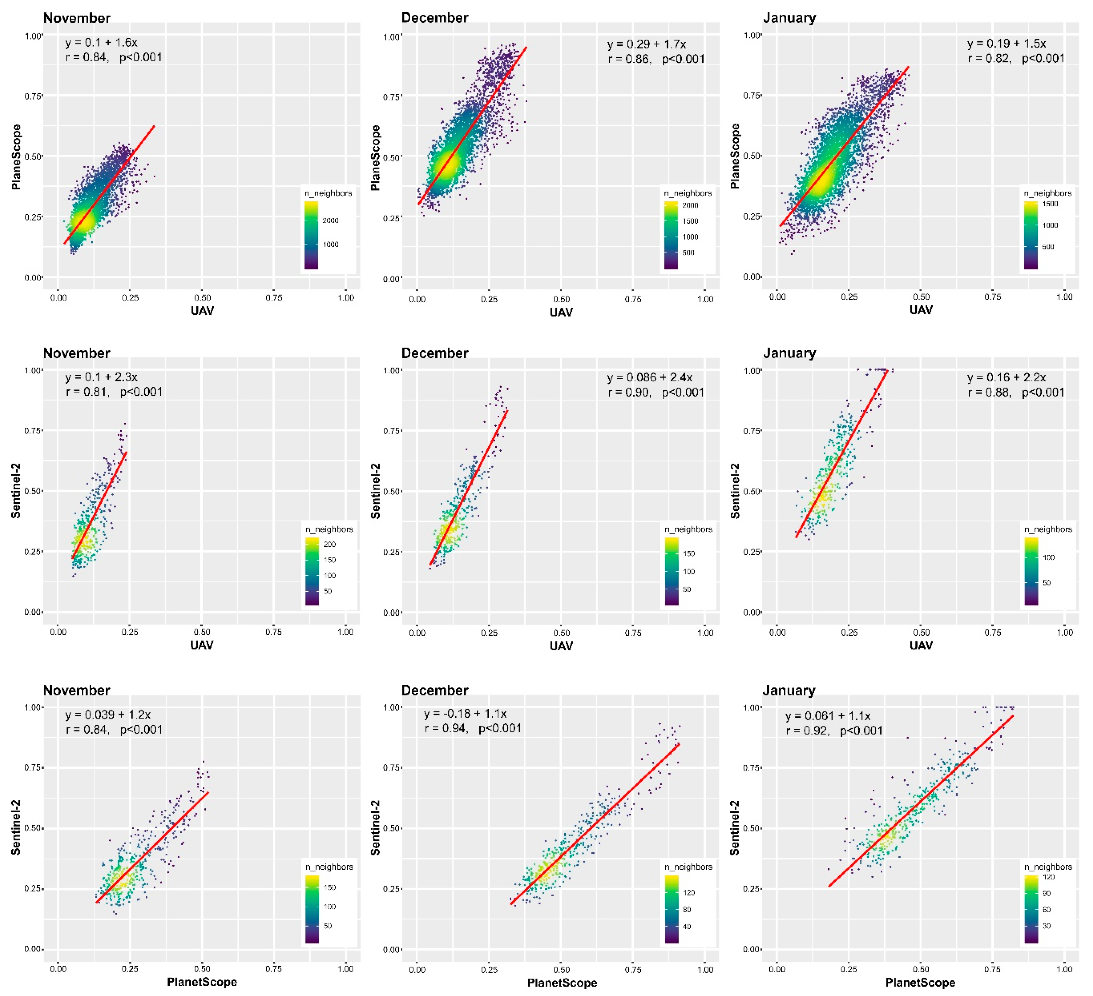
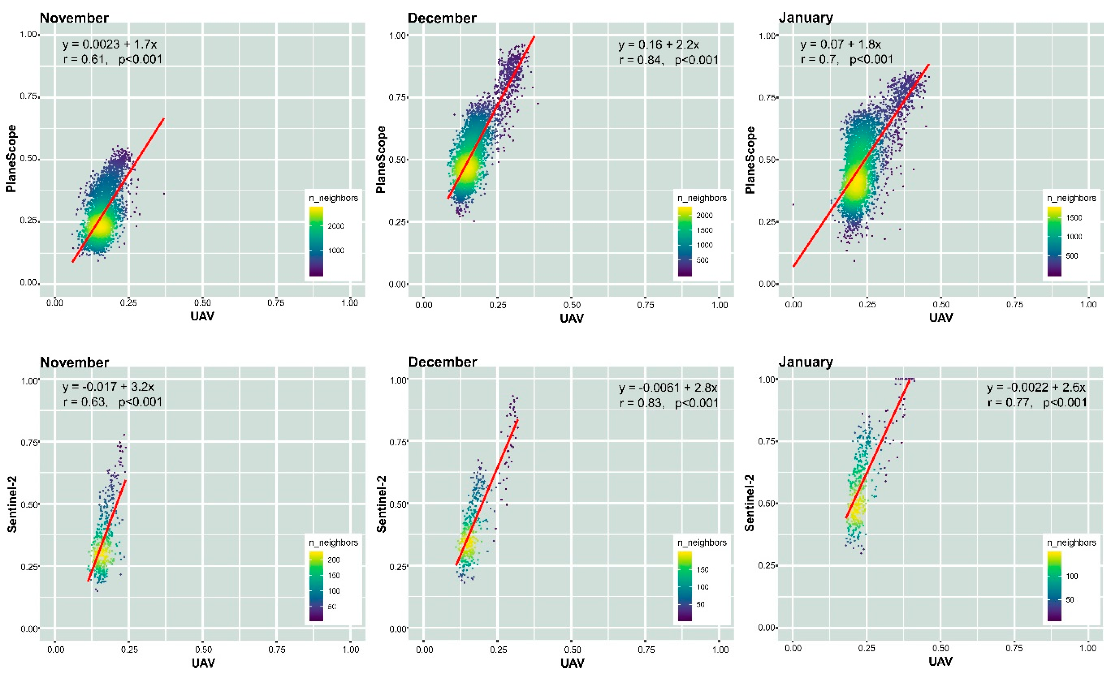
2.3. Comparison of Vegetation Indices (VIs) from the Three Platforms

In view of comparing satellite data with UAV data, three satellite images from each satellite platform were collected. Images were selected among those available without cloud cover in the days closest to those of the UAV surveys, as follows: 1) 29 November 2018, 19 December 2018, and 15 January 2019 from Sentinel-2 and 2) 23 November 2018, 19 December 2018, and 19 January 2019 from PlanetScope (Figure 2). The soil adjusted vegetation index (SAVI) was chosen to analyze the vegetative vigor of onion cultivation. SAVI was developed by Huete [63] to minimize the effects of soil background on the vegetation signal by inserting in the normalized difference vegetation index (NDVI) formula a constant soil adjustment factor L [64], according to the following formula:
S A V I = ( ρ N I R 1   ρ R e d ) ( ρ N I R 1 + ρ R e d + L ) ( 1 + L )
where L is the constant soil adjustment factor, and it can assume values between 0 and 1, depending on the level of vegetation cover, and ρ is the reflectance at the given wavelength.
The SAVI, belonging to the family of soil-corrected vegetation indices [65], is suitable to further reduce the background contribution reflectance by facilitating the identification of plants and their discrimination from the soil.
In this case study, the species monitored, onions, have thin and small leaves, especially in the early and middle stages of growth (mid-August-October, Figure 2), and in monitoring their growth, it is difficult to effectively extract the images from the background [16]. SAVI was calculated at the native MS band’s resolution of each sensor (5 cm for UAV, 3 m for PlanetScope, and 10 m for Sentinel-2). The various SAVI maps were used to describe and assess the variability within the onion field, as also shown in Khaliq et al. 2019 [66].
Descriptive statistics and histograms, calculated with R software, were used for a preliminary comparison of image data with native image resolutions. The degree of correlation between pairs of SAVI maps was then investigated using Pearson’s correlation coefficients. Initially, three comparisons were made taking into account the three dates investigated: a correlation between UAV (images resampled at 3 m resolution) and PlanetScope, a correlation between PlanetScope (images resampled at 10 m resolution) and Sentinel-2, and, finally, a correlation between UAV (images resampled at 10 m resolution) and Sentinel-2.
Then, to investigate the relationships between crop and soil cover, further correlation analyses were performed between the UAV SAVIs, including only onions and only soil and the SAVIs from the two satellite platforms.

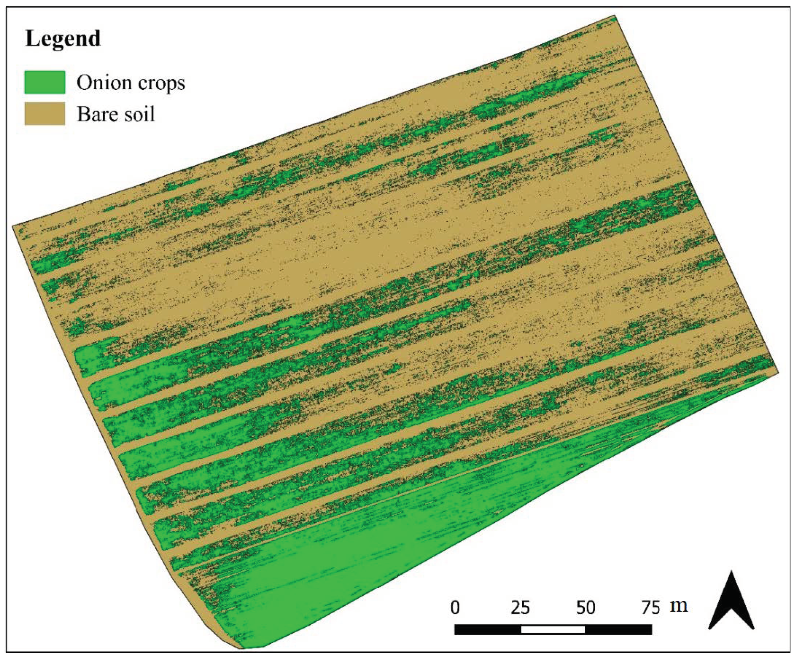
2.4. Image Segmentation and Classification

A GEOBIA process was developed to explore the potentiality of UAV images in discriminating soil coverage types and in producing other UAV SAVI maps for the subsequent comparison. Considering the type of crop and the structure of the field, which imply the presence of portions of soil, clearly visible from above, both among the plants and in the paths used for the passage of agricultural vehicles, classification was performed to separate crop and soil. Firstly, to extract the onion crop, the GEOBIA image classification procedure was performed. The classification was developed considering only the spectral response of the vegetation in the different bands. The first step performed in the GEOBIA procedure was the segmentation of the image. It is a fundamental prerequisite for classification/feature extraction [67] and foresees the segmentation of the image into separate, non-overlapping regions [68], then extracted in the form of vectorial objects.
Segmentation, which consists of dividing objects into smaller ones and creating new ones, altering the morphology of the previously existing ones, takes place according to precise rules. Segmentation’s algorithm used is the multiresolution algorithm [69].
This algorithm operates by identifying single objects, having a size of a pixel, and merging them with the nearby objects following a criterion of relative homogeneity while minimizing the average heterogeneity [70]. The homogeneity criterion is linked to the combination of the spectral and shape properties of the original image’s objects and of those of “new” objects obtained by the merging process. Homogeneity criteria are regulated by two parameters: shape and compactness.
The setting of the shape parameter concerns the importance\weight given by the segmentation process to the shape of objects with respect to color. The shape parameter can assume a value between 0 and 0.9. Color homogeneity derives from the standard deviation of spectral colors. Indeed, shape homogeneity results from the deviation of a compact (or smooth). Color and shape are linked, and the value or weight given by the user to the shape parameter determines different results of the segmentation.
In particular, the higher is the chosen value (between 0 and 0.9), the higher the influence of shape, with respect to the color, in the segmentation, and vice versa [71]. Compactness is the second adjustable parameter and determines the importance of shape with respect to the smoothness. It results in the product of width and length calculated on numbers of pixels [72]. The third parameter is the scale. The scale parameter determines the final size and dimension of the objects resulting from segmentation [67,73].
Attributing higher values or smaller values of scale parameter generates larger and smaller objects, respectively. Since the size of the objects depends on this parameter, it indirectly defines the maximum allowed heterogeneity for the obtained image objects. In addition, different weights can be attributed to the several input data (i.e., band layers). To perform the segmentation, the following parameters were chosen: 0.1 for shape, 0.5 for compactness, 0.3 for scale parameter, and weight 1 assigned to layers that correspond to the bands provided by Parrot Sequoia: Green, Red, Red Edge, and NIR.
Before choosing these parameters, some trial-and-error tests were performed, attributing different values to the segmentation parameters until the segmentation considered better (based on visual interpretation) was obtained. It was essential, in this case, to obtain segments that would allow the single plants to be distinguished.
After completing the segmentation phase, the onion crops were classified based only on a SAVI threshold value of ≥0.25. The value was chosen as a result of some trial-and-error tests and judged better based on visual interpretation of its ability to detect plants, following the methodology used in Modica et al. (2020) [74].
The data obtained concerning the vegetation coverage of the field was used to create a mask (and a second for the soil) to be applied to the map. The masks obtained by exporting a vector file containing only the class “onions” were applied to the UAV images at their native resolution with the aim to obtain only parts of orthomosaics concerning the onion crop.
In order to evaluate the presence of pure and mixed pixels of the vegetation class in Sentinel-2 and PlanetScope images, a spatial analysis procedure was developed in eCognition. First of all, shapefiles containing vector grids matching the pixel size of the Sentinel-2 and PlanetScope images were prepared on eCognition using a chessboard segmentation.
These grids were then superimposed on the classified UAV images at an upper level of the hierarchy. Several levels of segmentation constitute a hierarchical structure in the GEOBIA paradigm [75], and in our case, the super-objects (the grids) belonged to the upper level and included the vegetation class present in the lower level as a sub-object. Following this procedure, the area percentage occupied by the class “onion” within each pixel at Sentinel-2 and PlaneScope resolutions was calculated.

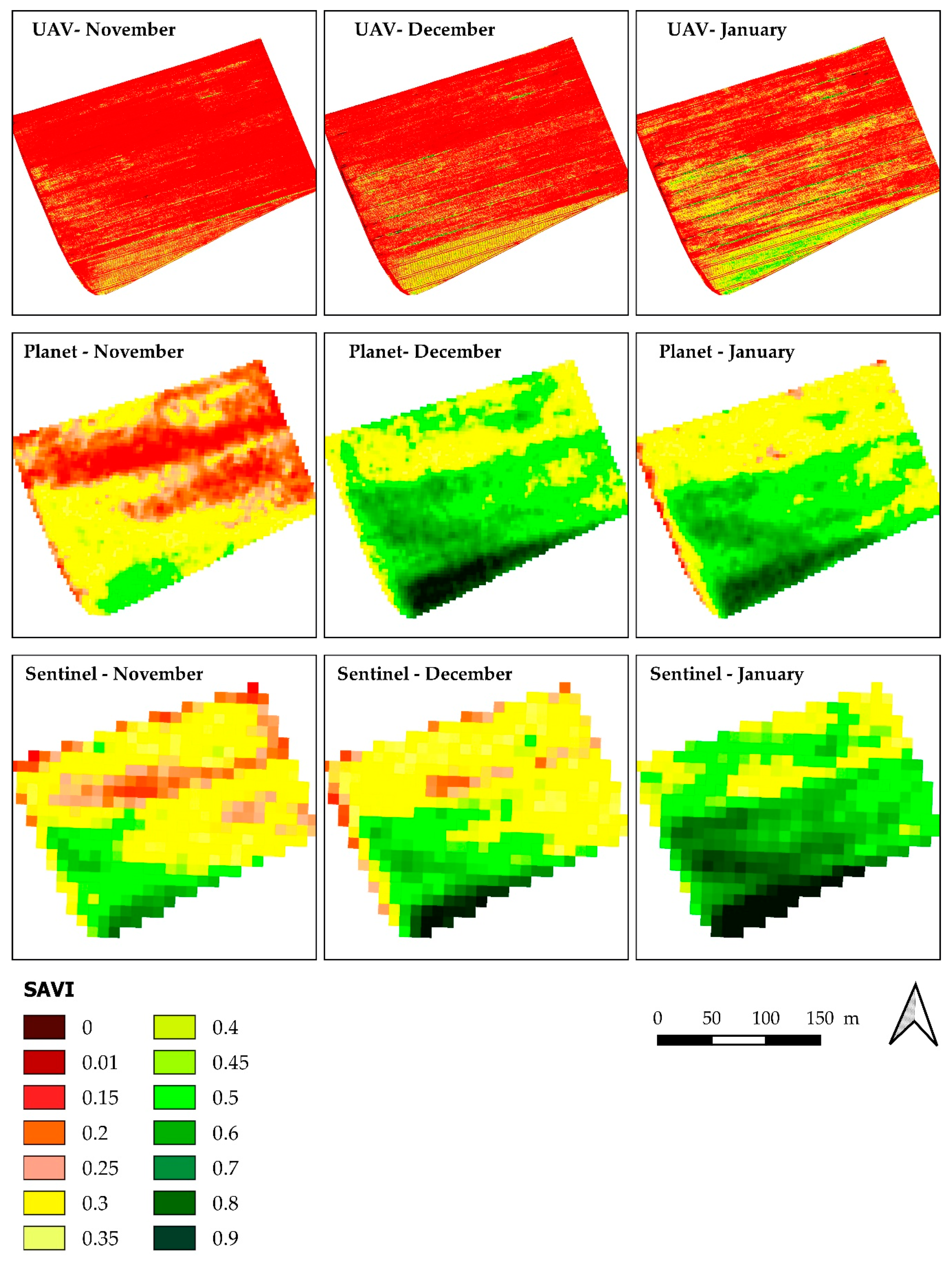
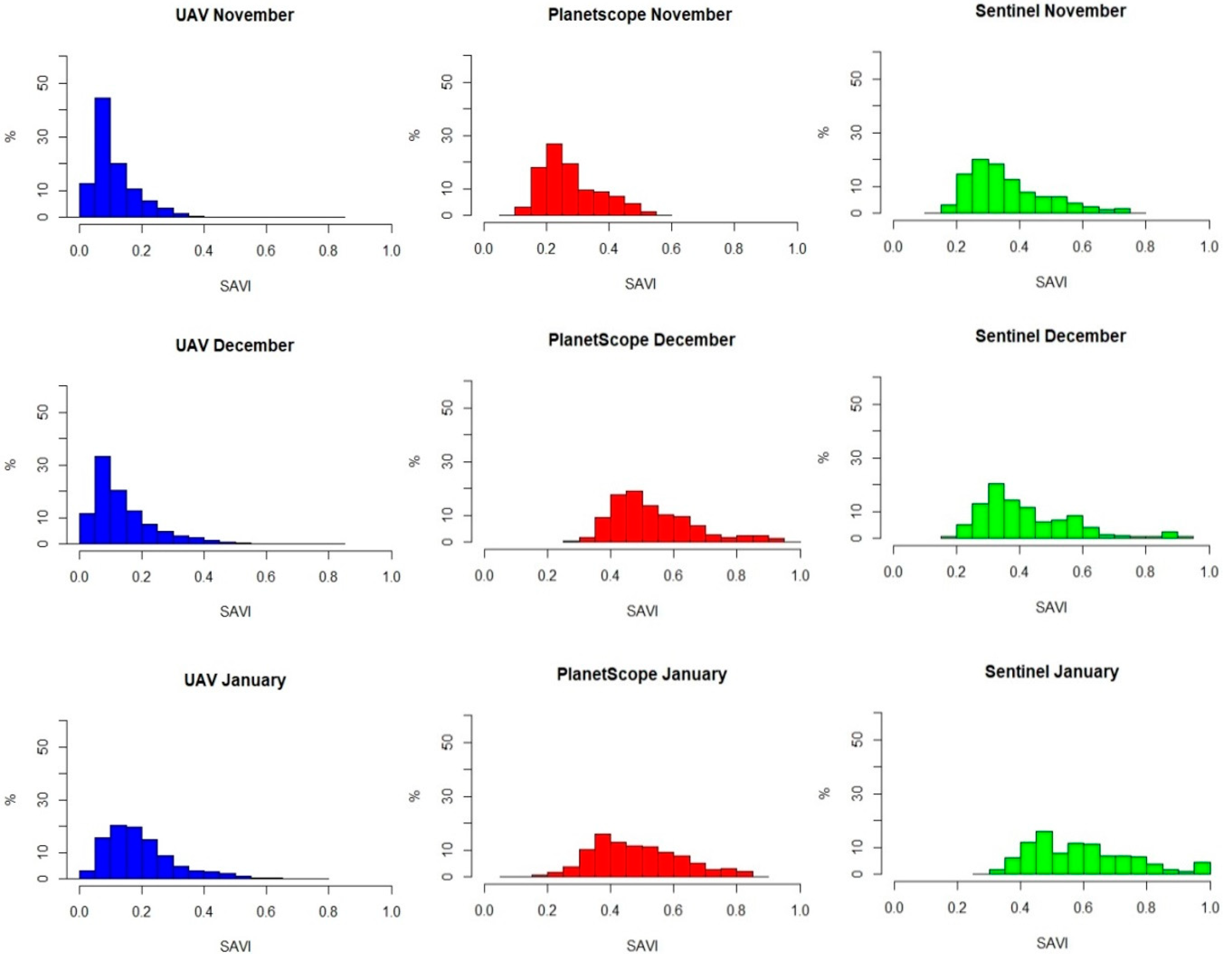
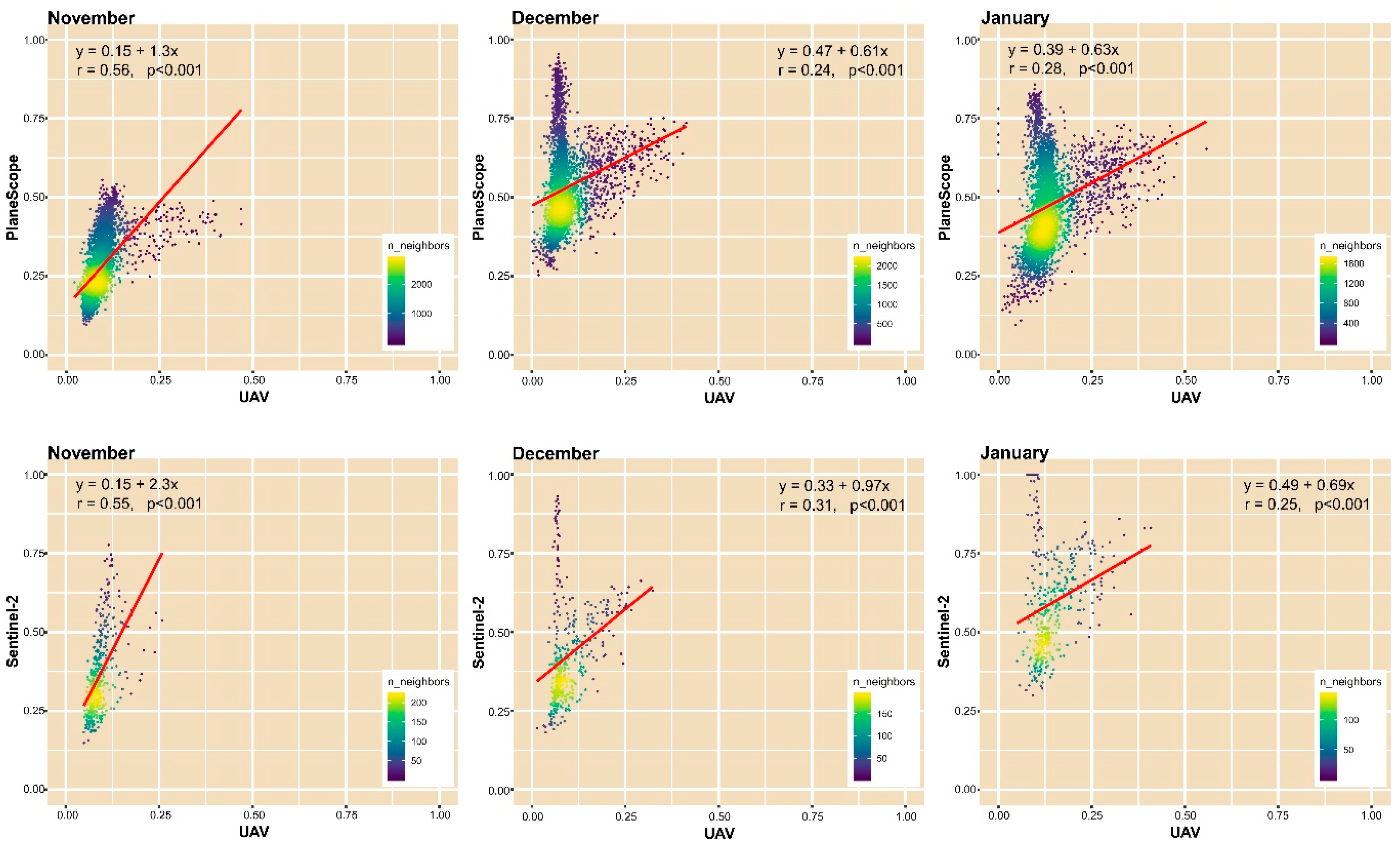
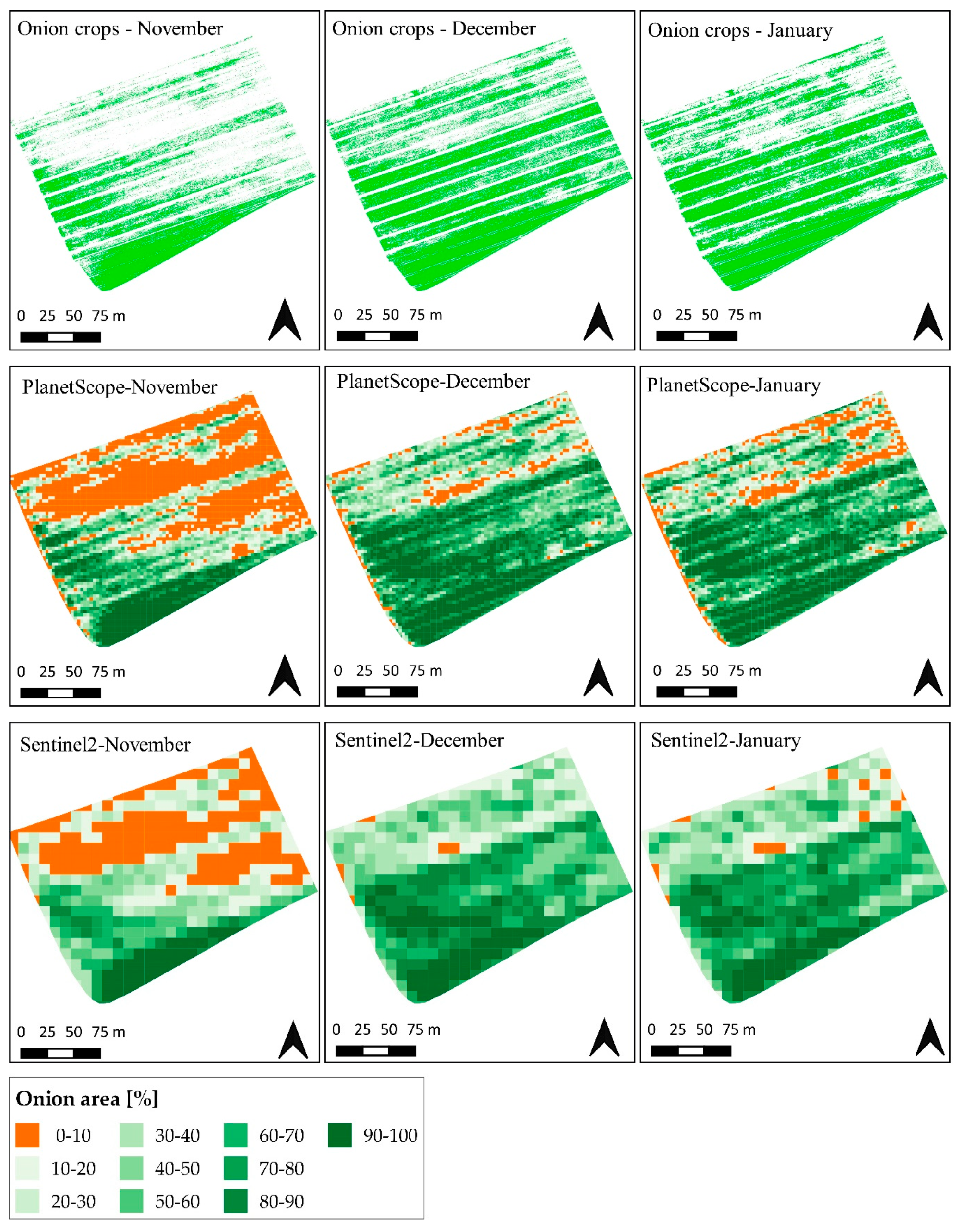
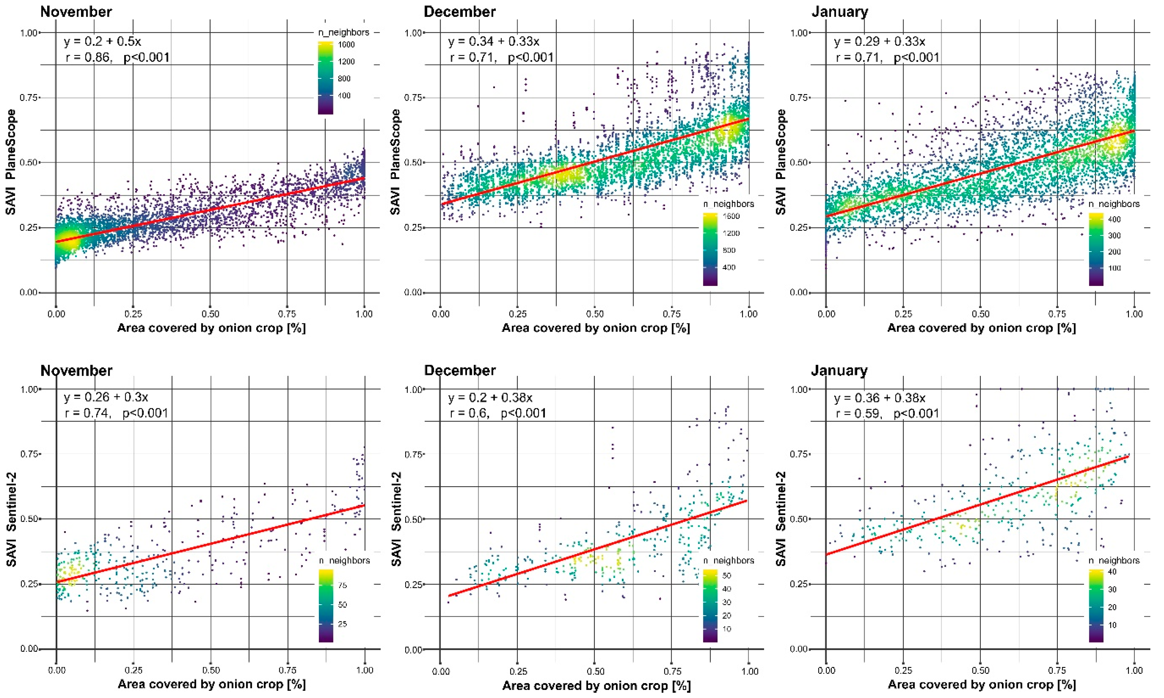
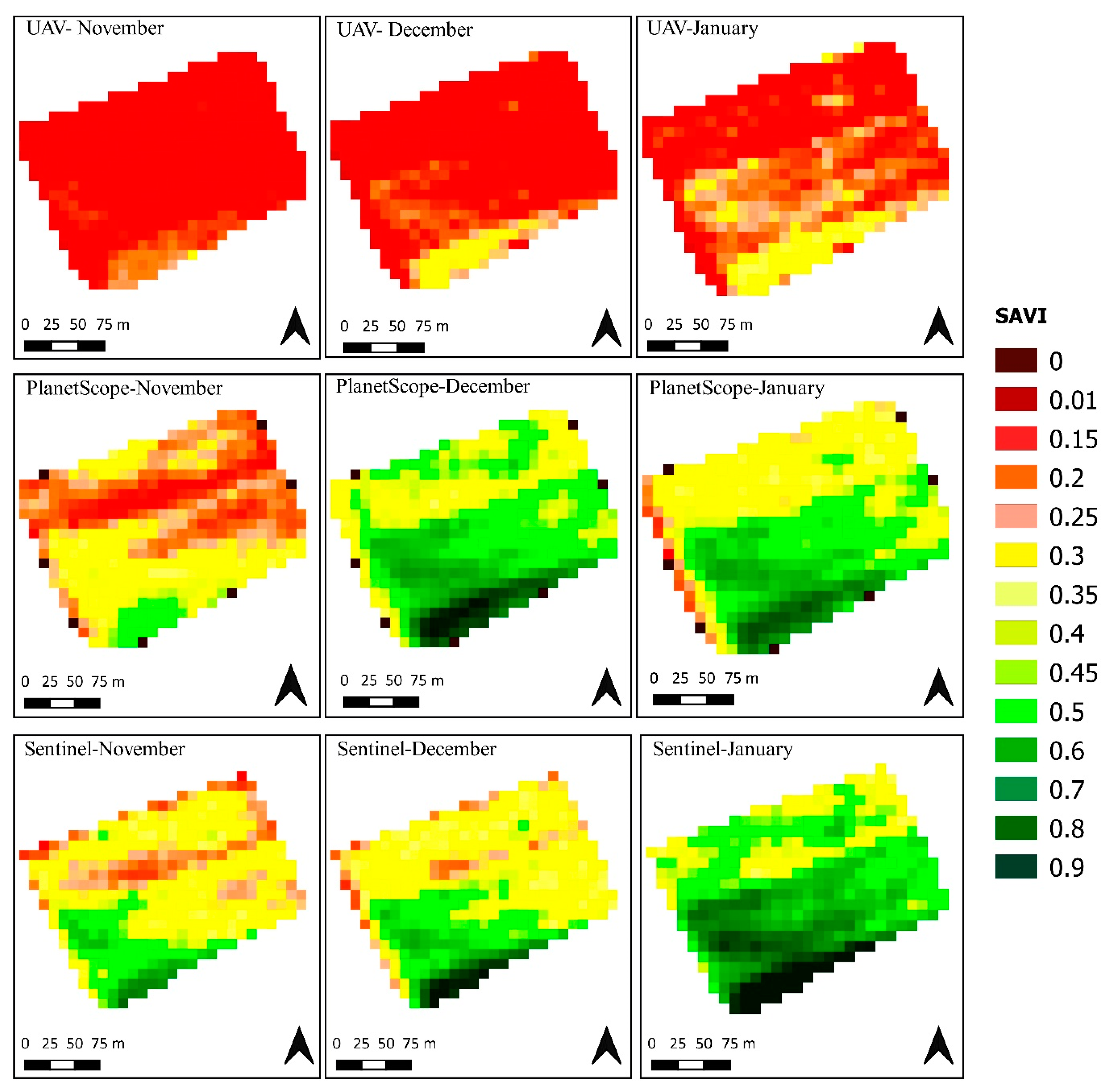
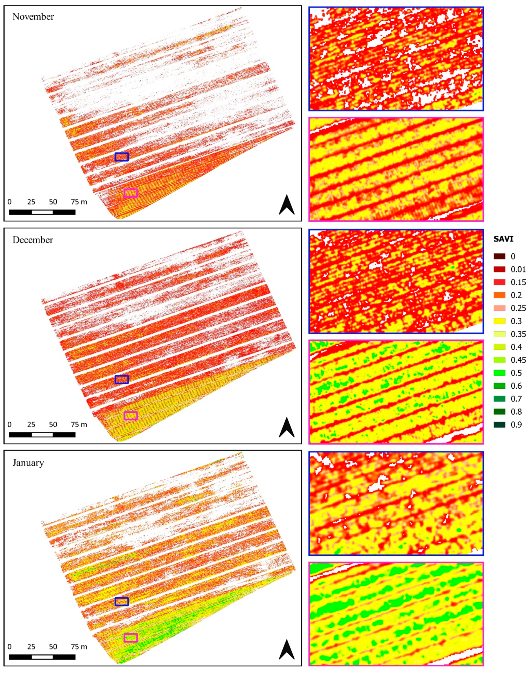
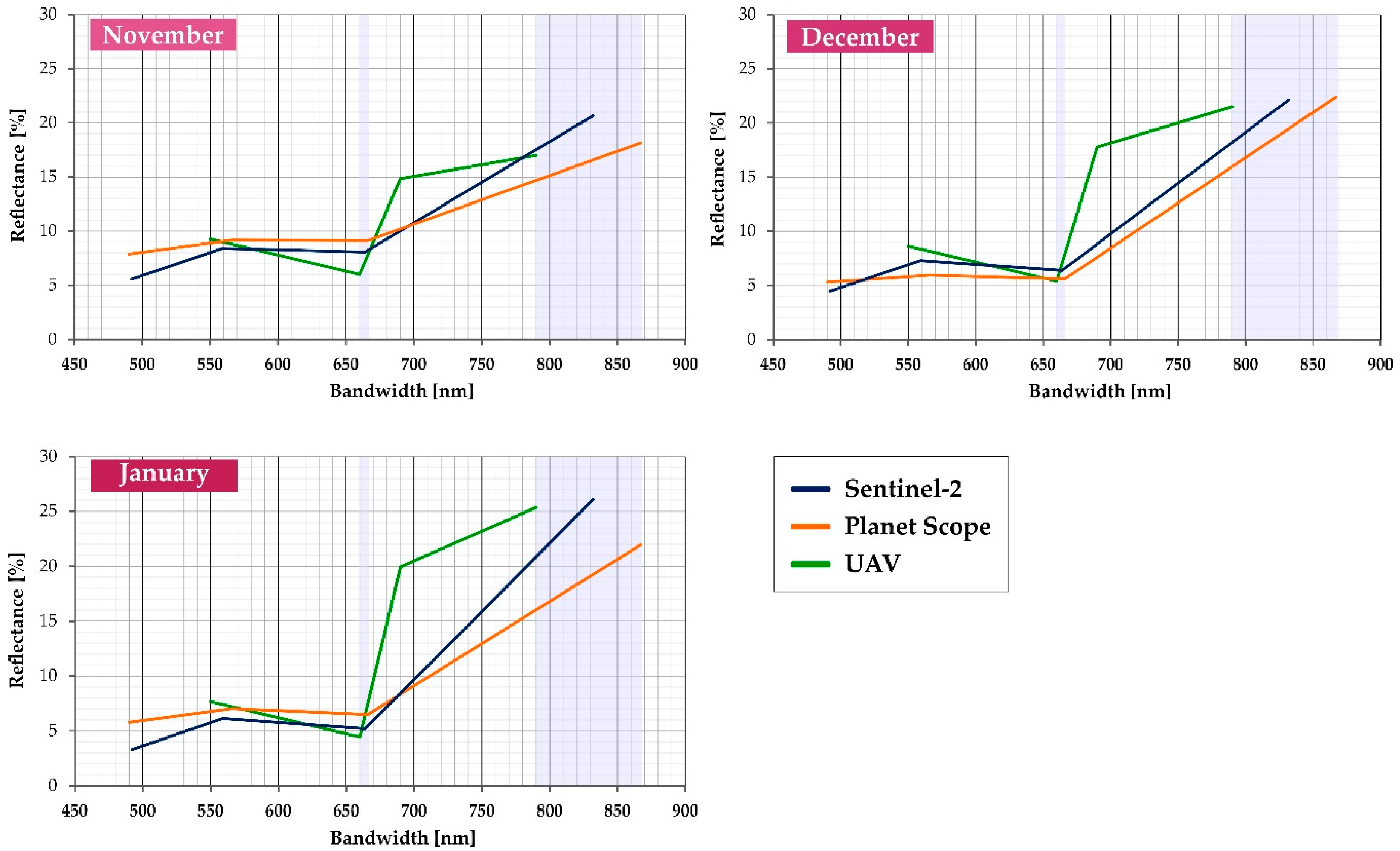
3. Results and Discussions

SAVI calculated at the native MS band’s resolution of each sensor is shown in Figure 4. Considering the imagery of November, UAV SAVI’s value ranged from 0 to 0.4, PlanetScope SAVI’s value ranged from 0.15 to 0.5, while Sentinel-2 SAVI’s value ranged from 0.15 to 0.8. In December, UAV SAVI’s value ranged from 0 to 0.7, PlanetScope SAVI’s value ranged from 0.3 to 0.9, and Sentinel-2 SAVI’s value ranged between 0.15 and 1.
Lastly, in January, as far as the UAV was concerned, the range was similar to that of the previous month, while SAVI’s value ranged between 0.15 and 0.8 and from 0.3 to 1 in PlanetScope and Sentinel-2, respectively.
The histograms reported in Figure 5 show the frequency distribution of SAVI values as a percentage of the total values and using the native resolution of each imagery. The histograms showed interesting differences between the three platforms used and differences also between the datasets of the same platforms. In general, histograms showed a reduced range of values in UAV images when compared to the broader ranges of Planetscope and, especially, Sentinel-2.
UAV SAVI average had values of 0.11, 0.14, and 0.19 in November, December, and January, respectively (Table 2). As for PlanetScope images, the mean value of the SAVI was 0.27, 0.53, and 0.48 in November, December, and January, respectively. In Sentinel-2 images, the mean value of the SAVI index was 0.36 in November, 0.42 in December, and 0.59 in January.
SAVI varied among different platforms, increasing its value from imagery with a higher resolution (UAV) to those with the lowest (Sentinel-2). However, even though the satellite and the UAV maps had different index ranges, it was possible to see some similarities in the distribution of vigor in the onion field. The SAVI values of UAV and PlanetScope showed a high correlation, with values between 0.82 and 0.86 (Figure 6). Similar correlations resulted from the comparisons with Sentinel-2 imagery.
This was highlighted by similarities in the localization of some areas of greater or lesser vigor of the field. This was evident by imagining to divide the image into two parts: in the upper part, there were areas of less vigor, while in the lower part, there were areas of the field with high vigor. Therefore, the satellites showed that they were capable of assessing the general conditions of the field.
However, it is essential to remember that the heterogeneity of the surfaces analyzed in terms of land cover (rows, inter-rows, and paths) and the spatial resolution of Sentinel-2 imagery implies that a single pixel is made up for the most part of rows, inter-rows, and paths used for the passage of agricultural machines [76].
Evaluating the spectral resolution of the three platforms, taking into account the coefficient of variation (CV), there was a clear difference between the CV of UAV images and that of satellites, as shown in Table 2. Considering the UAV imagery, CV had a value of 62% in November, 70% in December, and 55% in January, while the CV in satellite imagery ranged between 24% and 35% in the three months/datasets. In general, there was an increase in the CV in low (satellite) to high resolution (UAV) imagery. However, the increase in CV was not accompanied by a greater range of SAVI values in UAV images compared to those of the satellites. This was also confirmed by higher standard deviation values in satellite imagery than those of the UAV.
The onion crop surveyed is a highly heterogeneous crop characterized by the alternation of plants (higher values), inter-rows, and bare soil of background (lower values). The 5-cm very high-resolution of UAV images detected the oscillation of these values, allowing a distinction between plants and soil. On the other hand, the discontinuity between plants and bare soil was not detected by the lower satellites’ resolution that averages plants and bare soil reflectance values, therefore resulting in a narrow distribution.
Regarding the degree of correlation between pairs of SAVI maps based on Pearson’s correlation coefficients, observing the coherence between SAVI maps of the UAV (resampled at 3 m) and PlaneScope satellite platforms (Figure 6), high correlations emerged in the three months with r index values of 0.84 in November, 0.86 in December, and 0.82 in January. A similar correlation was found when comparing Sentinel-2 and UAV in November (0.81). Higher values were that of December and January, 0.9 and 0.88, respectively.
By comparing PlanetScope images with those of Sentinel-2, the highest correlation values could be observed in each month, compared to previous correlations with 0.84, 0.94, and 0.92 in November, December, and January, respectively. Indeed, even comparing visually at their respective resolutions (Figure 4), this was highlighted by similarities in the localization of some areas of greater or lesser vigor of the field.
The results obtained from the correlations of the UAV images, resampled first at 3 m and then at 10 m, seemed to indicate a certain coherence between the information provided by the three platforms.
With the aim of obtaining a more comprehensive picture of the analyzed crop, the SAVI index was also calculated by classifying the onion crop and the soil separately, using the UAV imagery as reference.
Therefore, we obtained, on the one hand, crop pixels (i.e., SAVI onions) and, on the other hand, bare soil pixels observed in the inter-rows and the paths (i.e., SAVI soil). This allowed taking into account the presence of mixed spectral pixels, dependent on the spatial resolution [77], and more evident, considering the size of the pixels compared to the object of study, in PlanetScope and Sentinel-2 images.
Then, further correlation analyses were performed to analyze the ability of platforms to provide information on crop and soil. Observing the correlation between SAVI onions and PlaneScope (Figure 7), values were 0.61 in November, 0.84 in December, and 0.7 in January. The analysis of the correlation between SAVI onions and Sentinel-2 (Figure 7) showed the following values: 0.63, 0.83, 0.77 in November, December, and January, respectively. The lower correlation in November values found with both satellites could be explained by a lower crop coverage compared to the soil, unlike December, where there was an increase in coverage.
Observing the correlation between SAVI soil and PlaneScope (Figure 8), values were 0.56 in November, 0.24 in December, and 0.28 in January. The analysis of the correlation between SAVI soil and Sentinel-2 (Figure 8) showed similar following values: 0.55, 0.31, 0.25 in November, December, and January, respectively. The correlation values in December and January were quite similar, while the highest value was found in November. This probably confirmed what was said before, considering that in November, the bare soil was prevalent within the scene compared to the crop. The results obtained confirmed what was shown in Khaliq et al., (2019) [66]. In particular, satellite imagery showed some limitations, indirectly providing reliable information concerning the status of the crops where the crop radiometric information can be altered by the presence of other sources like the soil, in this case, which in the month of November is predominant. In the following months, lower correlation values were due to a smaller presence of bare soil, compared to parts of the field completely covered or sporadically covered by the crop.
The aspect of the influence exerted by the different types of coverage on the pixel signal was related to spectral mixing pixels. This was a problem that concerned lower resolution images, i.e., those of PlanetScope and Sentinel-2. Using the onion class mask extracted from the UAV images, the percentage of area occupied by vegetation (onion) within the PlanetScope and Sentinel-2 pixels was calculated and is shown in Figure 9.
Pixels in orange contained a percentage of the pixel area occupied by vegetation between 0 and 10% and could be assimilated to pure pixels of bare soil. On the other hand, pixels in dark green could be assimilated, with a percentage of the pixel area occupied by vegetation between 90 and 100%, to pure pixels of vegetation. The remaining pixels, colored with different shades of green, were mixed pixels. A preponderant presence of orange pixels and, therefore, bare soil was easily visible in PlanetScope and Sentinel-2’s maps of November.
On the other hand, pure pixels of vegetation were mostly present in the maps of the following months, as a natural consequence of the course of the cultivation cycle. During these months, when the crop was regularly growing and the underlying soil cover capacity was improved, there were many pure pixels of vegetation. This happened especially in PlanetScope images, whose pixels covered an area of 9 m2 each. After all, the smaller the pixel size, the less likely it was that a pixel contained more coverage types. Fewer pure pixels were present in Sentinel-2 images, whose pixels had a size of 10 m × 10 m.
A correlation analysis between SAVI values and the percentage of area covered by onion crop within PlanetScope’s and Sentinel-2’s pixels was performed in order to deepen the aspect related to the presence of mixed pixels (Figure 10). Regarding PlanetScope images, the highest value was that of November with 0.86, probably explained by a predominant presence of pure pixels of bare soil. In the following months, the value obtained was 0.7; fewer pixels of bare soil were present, but the pure pixels of vegetation increased. This trend was similar in the correlation between Sentinel-2 images, but the values were lower: 0.74 in November, 0.6 in December, and 0.59 in January. In these images, the problem of mixed pixels was more pronounced.
Finally, we produced the SAVI maps using the images surveyed of the considered three months and for all the three platforms (Figure 11). With this aim, the UAV and PlanetScope maps were resampled at Sentinel-2’s 10 m geometrical resolution.
Looking at the map, the main effect of resampling UAV images was evident: the impossibility of distinguishing the details, which permit to discriminate among the crop, the soil, and the inter-rows. The resampling of the UAV images to a coarser spatial resolution, resulting in fewer pixels, had the loss of information related to the different SAVI values of rows, inter-rows, and paths as its main visible consequence. Indeed, the upscaling of spatial resolution has the consequence of erasing the details of the original data [78]. Increasing pixel size determines the decreasing of spatial variability of a vegetation index, as shown in Tarnavsky et al., (2008) [79]. Besides, radiometric resolution influenced VIs’ dynamic range. Indeed, observing SAVI in Figure 11, differences between platforms in the range of the index values appeared immediately evident. What was evident at first glance was the difference between the SAVI values of the UAV images when compared to the images of the two satellites, as a result of lower spectral variability in UAV images.
As far as UAV images were concerned, the lowest values were close to 0, while the highest values were 0.3 in November and December and 0.4 in January. Looking at the PlanetScope images instead, the highest values reached by the SAVI were 0.5, 0.9, and 0.8 in November, December, and January, respectively. In the Sentinel-2 images, there were minimum values higher than those of the other platforms, between 0.2 (from November) and 0.3 (in January). The maximum values reached by the SAVI were 0.7, 0.9, and 1 in November, December, and January, respectively. One important aspect must be stressed. The trend of the SAVI, proceeding from November, two months after the transplantation, until January, period close to the onion harvest, was the same regardless of the platform used. The same trend was confirmed by comparing the bands of the SAVI highlighted in the spectral signatures derived from pure pixels of onion in the three periods (see Figure A1 of the Appendix). The SAVI increased progressively from November to December and January.
This aspect appeared less apparent when looking at the UAV images resampled due to the loss of information. However, the SAVI calculated on the lower resolution images of the satellites had higher values from the dominant green color of the relevant vigor maps. While it is not clear how differences in spatial resolution affect VIs values under field conditions, some studies have demonstrated this effect by comparing different satellites [80,81,82,83,84,85], showing that VIs values are higher in coarser spatial resolution images. Factors responsible for inter-sensor VIs variations can be several [85]. Firstly, the calibration procedure may cause inter-sensor SAVI variations. Calibration provides precision and correctness to the data derived from a sensor so that all the datasets obtained from the same sensor can be compared. Algorithms used for calibration, including those useful for radiometric correction, are different between one sensor and another. These uncertainties remain when VIs produced by different sensors are compared [86,87]. However, as far as the calibration aspect is concerned, Sentinel-2’s images are better than PlanetScope [88]. Obviously, the technological differences between the sensors used by the UAVs and those present on the satellites cannot be ignored. Other variations can be due to the lack of bandwidth correspondence, as shown in Gallo and Daughtry (1987) [89] and Teillet et al., (1997) [90]. Besides, the differences in the spatial and radiometric resolution of the several sensors must also be taken into account [85]. Therefore, since there are several factors responsible for the differences between the sensors concerning the values of the vegetation indexes, it must be taken into account that these differences are not necessarily attributable to a single factor. It is rather prudent to consider all the cumulative effects of factors on VIs [85].
In addition to the maps with 10 m resolution, another was made, including the SAVI computed only on the onion crop. This was done in order to evaluate the contribution made by the UAV images. As shown, the UAV images proved useful for a separation between vegetation and soil due to obvious limitations (related to the size of individual plants) due to the spatial resolution of the satellites. The maps were produced using the masks produced on eCognition, already shown in Figure 12.
In particular, the masks obtained by exporting a vector file containing only the class “onions” were applied to the UAV images at their native resolution with the aim to obtain only parts of orthomosaics concerning onion crop. As a result, parts of the scene occupied by soil were excluded from the onion’s map.
Observing SAVI maps (Figure 13), applied to UAV images, considering only the part of the imagery occupied by onion crop, the index for three months surveyed was between 0 and 0.9.
The values for November were the lowest. This could be since the crop was still in the early stages of the cultivation cycle. Besides, during the segmentation phase, the software was not always able to correctly separate the vegetation from the background. It was conceivable that the lower values in the map could be traced back to the underlying terrain. Considering the map of December, the values were higher than the previous month. In the portion of the field where the transplant took place in mid-September, the index values were lower and were between 0.15 and 0.45. There were also evident areas where vegetation was challenging to grow, as shown in Messina et al. (2020) [52]. In the portion of the field in an advanced stage of cultivation, the values were higher. In particular, the values were between 0.45 and 0.9. The contrast of colors between the two areas of the field with different transplanting times was evident. The January map showed an increase in SAVI values where the crop was at a near harvest stage.
Vigor maps produced were useful to investigate areas of the field where the crop was struggling to grow, providing the farmer with potentially helpful information. Indeed, as shown in Figure 13, we could well distinguish areas (white, in the absence of data) where the crop seemed not to be present. In November, this area was higher than in the following months. Being in the month of November at the initial stages of growth, many plants, probably still too small, were not identified by the classification software, and also given the structure of the epigeal part of the onion, especially in this phase, would have required a resolution equal to or higher than 4 cm. In fact, in the month of December, many of the voids present in November were filled. However, some areas of the field, where the crop remained absent, were circled in black. These voids persisted in the month of January and were probably indicative of a problem of stunted growth due to several possible causes. These causes might be attributable to the action of abiotic agents, such as water stagnation, nutrient deficiency, or maybe the presence of a disease. In essence, beyond the values assumed by the index, the UAV had risen usefully and was able to identify the individual plants. Where this had not happened, we found voids. These voids could be explained either by the complete absence of the plants or by plants that were poorly cultivated or have had difficulty growing. So, this vigor map indirectly provides an indication to the farmer. This information could be used, for example, for localized fertilization or the grubbing up of diseased plants.
When comparing the strength maps of the different platforms, the satellites, considering the altitude in which they are located, provide images characterized by a coarser resolution but applicable for monitoring large areas and still able to recognize the variation in vegetation growth and health crop status [91]. In addition, as shown in this study, they are often characterized by a higher spectral variability and greater temporal and spatial reliability in the range of values assumed by the index, also taking into account a consolidated (in the case of Sentinel-2) calibration method. In addition, the SWIR band with which Sentinel-2 is equipped allows the calculation of other indices useful for monitoring, such as the normalized difference moisture index (NDMI) [92].
On the other hand, low altitude RS by using UAV is confirmed to be a useful tool in PA. In PA, considering agricultural monitoring, repeatable and timely information on variability within the field has a specific utility [3,93] as it allows to optimize production efficiency through sustainable and spatially explicit management practices [94,95]. In the present case study, some details of Figure 13 were made evident only by the vigor map derived from the UAV images. This is evident, given the inability of satellites to discriminate against specific details of the field, such as inter-row paths, as also shown in [49,66,96], which implies that the value of a VI within a pixel is necessarily derived from the average of the crop and inter-row information. It is also necessary to take into account the limits, due to their spatial resolution, which prevent satellites from highlighting problems located in areas whose area is less than the minimum identifiable by them.

4. Conclusions

This article dealt with a comparison between images of onion crops derived from three different platforms—a UAV and two satellites—one free medium resolution platform and the other low-cost, high-resolution platform. The comparison was mainly based on the analysis of the spatial resolution differences and the effects they may have on data quality in a PA context. For this reason, vigor maps were generated using the SAVI index and resampled at the lowest resolution of the satellite Sentinel-2.
Regarding the comparison between UAVs and satellites, the introduction of relatively new platforms, including nano-satellites, equipped with sensors that provide high or ultra-high resolution images, less than 3 m and 1 m, respectively, makes satellites increasingly competitive with UAVs in PA applications. The feature that makes the latter unique is that they can mount several types of sensors simultaneously [13]. Otherwise, considering all the platforms available, there is probably not yet one that can provide high spectral, spatial, and temporal resolution images [97]. Actually, simultaneous requirements for ultra-high spatial resolution images (<10 m) with almost daily time resolution can only be met by targeted acquisition via commercial programmable multi-sensor systems, such as WorldView, with an MS resolution of about 1 m. At the same time, Sentinel-2 is currently the finest resolution MS imaging mission in open source image data. In the case study, taking into account the characteristics of the crop, a resolution of less than or equal to one meter was preferable for more accurate data collection.
This article confirmed the results of other studies that have highlighted the role of high-resolution satellites in crop monitoring on a large scale. On the other hand, some limitations and uncertainties emerged in this case study where there is a need to discriminate localized conditions of inhomogeneity in the field, determined by abiotic or biotic stresses. This can be important in order to plan remedial interventions, such as localized application of pesticides, herbicides, and fertilizers. In this case, the images provided by UAVs made the difference, proving to be useful in guiding agronomic localized operations, such as fertilization and phytosanitary treatments. In the present case study, the monitoring regarded a crop, such as onion, characterized mainly in the early stages of the crop cycle by the small size and a non-homogeneous soil cover capacity. It is necessary to specify that better results in monitoring with UAVs could be obtained with higher resolution images than the one used; therefore, below 4 cm. As for a more accurate comparison of the quality of the data provided on the vegetation index values, it would be interesting to make a further comparison, in the same context, by including higher-priced cameras. Considering the overall results of the comparison carried out, it emerges that the contribution made by each platform must be regarded as complementary to that made by the other and not sufficient by itself in the accurate monitoring of the crop under study. This is true in light of the limitations shown by each platform.
Considering contexts similar to the one presented, the frequent use of the UAV for weekly monitoring could be uncomfortable and expensive if executed in several fields, perhaps not too large and spaced out from each other. In this regard, in these cases, it would be easier to use satellite images to check the general conditions of the field, interspersed with the use of more detailed UAV images at critical moments in the crop cycle. The advisable solution is not the use and preference of one platform over another. Therefore, a combination of different platforms, taking into account the level of information quality that each one can give, is desirable when the proper technical knowledge is available. In order to overcome the limitations of all the platforms described above, it would be desirable to combine UAV images (preferable with higher than 4 cm of resolution) with high-resolution satellite images to improve the overall quality of the final products. To be able to deepen the aspect related to the comparison between the different platforms, it would also be interesting to test the proposed approach on other crops.

Author Contributions

Conceptualization, supervision, G.M. (Giuseppe Modica); methodology, software, validation, G.M. (Gaetano Messina), J.M.P., M.V., and G.M. (Giuseppe Modica); investigation, data curation, visualization, writing—original draft, G.M. (Gaetano Messina) and G.M. (Giuseppe Modica); writing—review and editing, G.M. (Gaetano Messina), J.M.P., M.V., and G.M. (Giuseppe Modica). All authors have read and agreed to the published version of the manuscript.

Funding

The research of Dr. Jose M Peña was financed by the AGL2017-83325-C4-1R project (Spanish Ministry of Science, Innovation, and Universities and AEI/EU-FEDER funds).

Acknowledgments

The authors are grateful to DR-One S.r.l. (http://www.dr-onesrl.com—Belmonte Calabro, Cosenza, Italy) for providing UAV multispectral surveys and Azienda Agricola Ruggiero of Riccardo Ruggiero for granting us access to the area for the field surveys. We would like to thank the European Space Agency (ESA) for providing the Sentinel-2 data of the Copernicus Programme and the Planet Labs for the courtesy in providing the PlanetScope data used in this study.

Conflicts of Interest

The authors declare no conflict of interest.

Appendix A

Figure A1. The spectral signature of onion crop derived from the reflectance data of pure onion pixels for the three platforms in the three periods surveyed (November, December, and January). The shaded light violet indicates the region of the two bands used for the soil adjusted vegetation index (SAVI) calculation (red and near-infrared, NIR).
Remotesensing 12 03424 g0a1

References

  1. Solano, F.; Di Fazio, S.; Modica, G. A methodology based on GEOBIA and WorldView-3 imagery to derive vegetation indices at tree crown detail in olive orchards. Int. J. Appl. Earth Obs. Geoinf. 2019, 83, 101912. [Google Scholar] [CrossRef]
  2. Mulla, D.J. Twenty five years of remote sensing in precision agriculture: Key advances and remaining knowledge gaps. Biosyst. Eng. 2013, 114, 358–371. [Google Scholar] [CrossRef]
  3. Moran, M.S.; Inoue, Y.; Barnes, E.M. Opportunities and limitations for image-based remote sensing in precision crop management. Remote Sens. Environ. 1997, 61, 319–346. [Google Scholar] [CrossRef]
  4. Sagan, V.; Maimaitijiang, M.; Sidike, P.; Eblimit, K.; Peterson, K.T.; Hartling, S.; Esposito, F.; Khanal, K.; Newcomb, M.; Pauli, D.; et al. UAV-based high resolution thermal imaging for vegetation monitoring, and plant phenotyping using ICI 8640 P, FLIR Vue Pro R 640, and thermomap cameras. Remote Sens. 2019, 11, 330. [Google Scholar] [CrossRef] [Green Version]
  5. Messina, G.; Modica, G. Applications of UAV thermal imagery in precision agriculture: State of the art and future research outlook. Remote Sens. 2020, 12, 1491. [Google Scholar] [CrossRef]
  6. McCabe, M.F.; Houborg, R.; Lucieer, A. High-resolution sensing for precision agriculture: From Earth-observing satellites to unmanned aerial vehicles. Remote Sens. Agric. Ecosyst. Hydrol. XVIII 2016, 9998, 999811. [Google Scholar] [CrossRef] [Green Version]
  7. ESA. Resolution and Swath. Available online: earth.esa.int/web/sentinel/missions/sentinel-2/instrument-payload/resolution-and-swath (accessed on 2 April 2020).
  8. Vizzari, M.; Santaga, F.; Benincasa, P. Sentinel 2-Based Nitrogen VRT Fertilization in Wheat: Comparison between Traditional and Simple Precision Practices. Agronomy 2019, 9, 278. [Google Scholar] [CrossRef] [Green Version]
  9. Modica, G.; Pollino, M.; Solano, F. Sentinel-2 Imagery for Mapping Cork Oak (Quercus suber L.) Distribution in Calabria (Italy): Capabilities and Quantitative Estimation. In New Metropolitan Perspectives; ISHT Smart Innovation, Systems and Technologies; Calabrò, F., Della Spina, L., Bevilacqua, C., Eds.; Springer: Cham, Switzerland, 2019; Volume 100, pp. 60–67. ISBN 9783319920993. [Google Scholar]
  10. Houborg, R.; McCabe, M.F. High-Resolution NDVI from planet’s constellation of earth observing nano-satellites: A new data source for precision agriculture. Remote Sens. 2016, 8, 768. [Google Scholar] [CrossRef] [Green Version]
  11. Colomina, I.; Molina, P. Unmanned aerial systems for photogrammetry and remote sensing: A review. ISPRS J. Photogramm. Remote Sens. 2014, 92, 79–97. [Google Scholar] [CrossRef] [Green Version]
  12. Zhang, C.; Kovacs, J.M. The application of small unmanned aerial systems for precision agriculture: A review. Precis. Agric. 2012, 13, 693–712. [Google Scholar] [CrossRef]
  13. Maes, W.H.; Steppe, K. Perspectives for Remote Sensing with Unmanned Aerial Vehicles in Precision Agriculture. Trends Plant Sci. 2019, 24, 152–164. [Google Scholar] [CrossRef]
  14. Khanal, S.; Fulton, J.; Shearer, S. An overview of current and potential applications of thermal remote sensing in precision agriculture. Comput. Electron. Agric. 2017, 139, 22–32. [Google Scholar] [CrossRef]
  15. He, Y.; Weng, Q. High Spatial Resolution Remote Sensing: Data, Analysis, and Applications; CRC Press: Boca Raton, FL, USA, 2018; ISBN 9780429470196. [Google Scholar]
  16. Jeong, S.; Kim, D.; Yun, H.; Cho, W.; Kwon, Y.; Kim, H. Monitoring the growth status variability in Onion (Allium cepa) and Garlic (Allium sativum) with RGB and multi-spectral UAV remote sensing imagery. In Proceedings of the 7th Asian-Australasian Conference on Precision Agriculture, Hamilton, New Zealand, 16–18 October 2017; pp. 1–6. [Google Scholar]
  17. Tang, C.; Turner, N.C. The influence of alkalinity and water stress on the stomatal conductance, photosynthetic rate and growth of Lupinus angustifolius L. and Lupinus pilosus Murr. Aust. J. Exp. Agric. 1999, 39, 457–464. [Google Scholar] [CrossRef]
  18. Benincasa, P.; Antognelli, S.; Brunetti, L.; Fabbri, C.A.; Natale, A.; Sartoretti, V.; Modeo, G.; Guiducci, M.; Tei, F.; Vizzari, M. Reliability of Ndvi Derived By High Resolution Satellite and Uav Compared To in-Field Methods for the Evaluation of Early Crop N Status and Grain Yield in Wheat. Exp. Agric. 2017, 1–19. [Google Scholar] [CrossRef]
  19. Yao, H.; Qin, R. Unmanned Aerial Vehicle for Remote Sensing Applications—A Review. Remote Sens. 2019, 11, 1–22. [Google Scholar] [CrossRef]
  20. Blaschke, T. Object based image analysis for remote sensing. ISPRS J. Photogramm. Remote Sens. 2010, 65, 2–16. [Google Scholar] [CrossRef] [Green Version]
  21. Blaschke, T.; Hay, G.J.; Kelly, M.; Lang, S.; Hofmann, P.; Addink, E.; Queiroz Feitosa, R.; van der Meer, F.; van der Werff, H.; van Coillie, F.; et al. Geographic Object-Based Image Analysis—Towards a new paradigm. ISPRS J. Photogramm. Remote Sens. 2014, 87, 180–191. [Google Scholar] [CrossRef] [Green Version]
  22. Chen, G.; Weng, Q.; Hay, G.J.; He, Y. Geographic object-based image analysis (GEOBIA): Emerging trends and future opportunities. GISci. Remote Sens. 2018, 55, 159–182. [Google Scholar] [CrossRef]
  23. Belgiu, M.; Csillik, O. Sentinel-2 cropland mapping using pixel-based and object-based time-weighted dynamic time warping analysis. Remote Sens. Environ. 2018, 204, 509–523. [Google Scholar] [CrossRef]
  24. Csillik, O.; Cherbini, J.; Johnson, R.; Lyons, A.; Kelly, M. Identification of Citrus Trees from Unmanned Aerial Vehicle Imagery Using Convolutional Neural Networks. Drones 2018, 2, 39. [Google Scholar] [CrossRef] [Green Version]
  25. De Castro, A.I.; Torres-Sánchez, J.; Peña, J.M.; Jiménez-Brenes, F.M.; Csillik, O.; López-Granados, F. An automatic random forest-OBIA algorithm for early weed mapping between and within crop rows using UAV imagery. Remote Sens. 2018, 10, 285. [Google Scholar] [CrossRef] [Green Version]
  26. De Castro, A.I.; Peña, J.M.; Torres-Sánchez, J.; Jiménez-Brenes, F.; López-Granados, F. Mapping Cynodon dactylon in vineyards using UAV images for site-specific weed control. Adv. Anim. Biosci. 2017, 8, 267–271. [Google Scholar] [CrossRef]
  27. López-Granados, F.; Torres-Sánchez, J.; De Castro, A.I.; Serrano-Pérez, A.; Mesas-Carrascosa, F.J.; Peña, J.M. Object-based early monitoring of a grass weed in a grass c rop using high resolution UAV imagery. Agron. Sustain. Dev. 2016, 36, 1–12. [Google Scholar] [CrossRef]
  28. Ok, A.O.; Ozdarici-Ok, A. 2-D delineation of individual citrus trees from UAV-based dense photogrammetric surface models. Int. J. Digit. Earth 2018, 11, 583–608. [Google Scholar] [CrossRef]
  29. Ozdarici-Ok, A. Automatic detection and delineation of citrus trees from VHR satellite imagery. Int. J. Remote Sens. 2015, 36, 4275–4296. [Google Scholar] [CrossRef]
  30. Torres-Sánchez, J.; López-Granados, F.; Peña, J.M. An automatic object-based method for optimal thresholding in UAV images: Application for vegetation detection in herbaceous crops. Comput. Electron. Agric. 2015, 114, 43–52. [Google Scholar] [CrossRef]
  31. De Castro, A.I.; Jiménez-Brenes, F.M.; Torres-Sánchez, J.; Peña, J.M.; Borra-Serrano, I.; López-Granados, F. 3-D characterization of vineyards using a novel UAV imagery-based OBIA procedure for precision viticulture applications. Remote Sens. 2018, 10, 584. [Google Scholar] [CrossRef] [Green Version]
  32. Peña, J.M.; Kelly, M.; De Castro, A.I.; López Granados, F. Object-based approach for crop row characterization in UAV images for site-specific weed management. In Proceedings of the 4th International Conference on Geographic Object-Based Image Analysis (GEOBIA 2012), Rio Janeiro, Brazil, 7–9 May 2012; Queiroz-Feitosa, A., Ed.; pp. 426–430. [Google Scholar]
  33. Córcoles, J.I.; Ortega, J.F.; Hernández, D.; Moreno, M.A. Estimation of leaf area index in onion (Allium cepa L.) using an unmanned aerial vehicle. Biosyst. Eng. 2013, 115, 31–42. [Google Scholar] [CrossRef]
  34. Ballesteros, R.; Ortega, J.F.; Hernandez, D.; Moreno, M.A. Onion biomass monitoring using UAV-based RGB imaging. Precis. Agric. 2018, 1–18. [Google Scholar] [CrossRef]
  35. Aboukhadrah, S.H.; El—Alsayed, A.W.A.H.; Sobhy, L.; Abdelmasieh, W. Response of Onion Yield and Quality To Different Planting Date, Methods and Density. Egypt. J. Agron. 2017, 39, 203–219. [Google Scholar] [CrossRef]
  36. Mallor, C.; Balcells, M.; Mallor, F.; Sales, E. Genetic variation for bulb size, soluble solids content and pungency in the Spanish sweet onion variety Fuentes de Ebro. Response to selection for low pungency. Plant Breed. 2011, 130, 55–59. [Google Scholar] [CrossRef] [Green Version]
  37. Ranjitkar, H. A Handbook of Practical Botany; Ranjitkar, A.K., Ed.; Kathmandu Publishing: Kathmandu, Nepal, 2003. [Google Scholar]
  38. Pareek, S.; Sagar, N.A.; Sharma, S.; Kumar, V. Onion (Allium cepa L.). In Fruit and Vegetable Phytochemicals: Chemistry and Human Health; Yahia, E.M., Ed.; Wiley & Sons: Hoboken, NJ, USA, 2017. [Google Scholar]
  39. Zhao, L.; Shi, Y.; Liu, B.; Hovis, C.; Duan, Y.; Shi, Z. Finer Classification of Crops by Fusing UAV Images and Sentinel-2A Data. Remote Sens. 2019, 11, 12. [Google Scholar] [CrossRef] [Green Version]
  40. Bernardi, B.; Zimbalatti, G.; Proto, A.R.; Benalia, S.; Fazari, A.; Callea, P. Mechanical grading in PGI Tropea red onion post harvest operations. J. Agric. Eng. 2013, 44, 317–322. [Google Scholar] [CrossRef]
  41. Tiberini, A.; Mangano, R.; Micali, G.; Leo, G.; Manglli, A.; Tomassoli, L.; Albanese, G. Onion yellow dwarf virus ∆∆Ct-based relative quantification obtained by using real-time polymerase chain reaction in “Rossa di Tropea” onion. Eur. J. Plant Pathol. 2019, 153, 251–264. [Google Scholar] [CrossRef]
  42. Consorzio di Tutela della Cipolla Rossa di Tropea Calabria IGP. Available online: www.consorziocipollatropeaigp.com (accessed on 30 April 2020).
  43. Meier, U. Growth Stages of Mono- and Dicotyledonous Plants; Federal Biological Research Centre for Agriculture and Forestry, Ed.; Blackwell Wissenschafts-Verlag: Berlin, Germany, 2001; Volume 12, ISBN 9783826331527. [Google Scholar]
  44. Bukowiecki, J.; Rose, T.; Ehlers, R.; Kage, H. High-Throughput Prediction of Whole Season Green Area Index in Winter Wheat With an Airborne Multispectral Sensor. Front. Plant Sci. 2020, 10, 1. [Google Scholar] [CrossRef] [PubMed]
  45. Iqbal, F.; Lucieer, A.; Barry, K. Poppy crop capsule volume estimation using UAS remote sensing and random forest regression. Int. J. Appl. Earth Obs. Geoinf. 2018, 73, 362–373. [Google Scholar] [CrossRef]
  46. Maimaitijiang, M.; Ghulam, A.; Sidike, P.; Hartling, S.; Maimaitiyiming, M.; Peterson, K.; Shavers, E.; Fishman, J.; Peterson, J.; Kadam, S.; et al. Unmanned Aerial System (UAS)-based phenotyping of soybean using multi-sensor data fusion and extreme learning machine. ISPRS J. Photogramm. Remote Sens. 2017, 134, 43–58. [Google Scholar] [CrossRef]
  47. Fawcett, D.; Panigada, C.; Tagliabue, G.; Boschetti, M.; Celesti, M.; Evdokimov, A.; Biriukova, K.; Colombo, R.; Miglietta, F.; Rascher, U.; et al. Multi-Scale Evaluation of Drone-Based Multispectral Surface Reflectance and Vegetation Indices in Operational Conditions. Remote Sens. 2020, 12, 514. [Google Scholar] [CrossRef] [Green Version]
  48. Jorge, J.; Vallbé, M.; Soler, J.A. Detection of irrigation inhomogeneities in an olive grove using the NDRE vegetation index obtained from UAV images vegetation index obtained from UAV images. Eur. J. Remote Sens. 2019, 52, 169–177. [Google Scholar] [CrossRef] [Green Version]
  49. Pádua, L.; Marques, P.; Adão, T.; Guimarães, N.; Sousa, A.; Peres, E.; Sousa, J.J. Vineyard Variability Analysis through UAV-Based Vigour Maps to Assess Climate Change Impacts. Agronomy 2019, 9, 581. [Google Scholar] [CrossRef] [Green Version]
  50. Deng, L.; Mao, Z.; Li, X.; Hu, Z.; Duan, F.; Yan, Y. UAV-based multispectral remote sensing for precision agriculture: A comparison between different cameras. ISPRS J. Photogramm. Remote Sens. 2018, 146, 124–136. [Google Scholar] [CrossRef]
  51. Cubero-Castan, M.; Schneider-Zapp, K.; Bellomo, M.; Shi, D.; Rehak, M.; Strecha, C. Assessment Of The Radiometric Accuracy In A Target Less Work Flow Using Pix4D Software. In Proceedings of the 2018 9th Workshop on Hyperspectral Image and Signal Processing: Evolution in Remote Sensing (WHISPERS), Amsterdam, The Netherlands, 23–26 September 2018; Volume 2018, pp. 1–4. [Google Scholar]
  52. Messina, G.; Fiozzo, V.; Praticò, S.; Siciliani, B.; Curcio, A.; Di Fazio, S.; Modica, G. Monitoring Onion Crops Using Multispectral Imagery from Unmanned Aerial Vehicle (UAV). In Proceedings of the “NEW METROPOLITAN PERSPECTIVES. Knowledge Dynamics and Innovation-driven Policies Towards Urban and Regional Transition”, Reggio Calabria, Italy, 18–23 May 2020; Bevilacqua, C., Francesco, C., Della Spina, L., Eds.; Springer: Reggio Calabria, Italy, 2020; Volume 2, pp. 1640–1649. [Google Scholar]
  53. Messina, G.; Praticò, S.; Siciliani, B.; Curcio, A.; Di Fazio, S.; Modica, G. Telerilevamento multispettrale da drone per il monitoraggio delle colture in agricoltura di precisione. Un’applicazione alla cipolla rossa di Tropea (Multispectral UAV remote sensing for crop monitoring in precision farming. An application to the Red onion of Tropea). LaborEst 2020, 21. in press. [Google Scholar]
  54. Bartsch, A.; Widhalm, B.; Leibman, M.; Ermokhina, K.; Kumpula, T.; Skarin, A.; Wilcox, E.J.; Jones, B.M.; Frost, G.V.; Höfler, A.; et al. Feasibility of tundra vegetation height retrieval from Sentinel-1 and Sentinel-2 data. Remote Sens. Environ. 2020, 237, 111515. [Google Scholar] [CrossRef]
  55. Yang, X.; Zhao, S.; Qin, X.; Zhao, N.; Liang, L. Mapping of urban surface water bodies from sentinel-2 MSI imagery at 10 m resolution via NDWI-based image sharpening. Remote Sens. 2017, 9, 596. [Google Scholar] [CrossRef] [Green Version]
  56. Spoto, F.; Martimort, P.; Drusch, M. Sentinel—2: ESA’s Optical High-Resolution Mission for GMES Operational Services; Elsevier: Amsterdam, The Netherlands, 2012; Volume 707 SP. ISBN 9789290922711. [Google Scholar]
  57. Rapinel, S.; Mony, C.; Lecoq, L.; Clément, B.; Thomas, A.; Hubert-Moy, L. Evaluation of Sentinel-2 time-series for mapping floodplain grassland plant communities. Remote Sens. Environ. 2019, 223, 115–129. [Google Scholar] [CrossRef]
  58. Copernicus. Available online: scihub.copernicus.eu (accessed on 15 April 2020).
  59. Planet Team. Planet Application Program Interface: In Space for Life on Earth; Planet Team: San Francisco, CA, USA, 2017; Available online: https://api. planet.com (accessed on 30 April 2020).
  60. Ghuffar, S. DEM generation from multi satellite Planetscope imagery. Remote Sens. 2018, 10, 1462. [Google Scholar] [CrossRef] [Green Version]
  61. Kääb, A.; Altena, B.; Mascaro, J. Coseismic displacements of the 14 November 2016 Mw 7.8 Kaikoura, New Zealand, earthquake using the Planet optical cubesat constellation. Nat. Hazards Earth Syst. Sci. 2017, 17, 627–639. [Google Scholar] [CrossRef] [Green Version]
  62. Planet Labs Inc. Planet Imagery and Archive. Available online: https://www.planet.com/products/planet-imagery/ (accessed on 30 April 2020).
  63. Huete, A.R. A soil-adjusted vegetation index (SAVI). Remote Sens. Environ. 1988, 25, 295–309. [Google Scholar] [CrossRef]
  64. Taylor, P.; Silleos, N.G. Vegetation Indices: Advances Made in Biomass Estimation and Vegetation Monitoring in the Last 30 Years Vegetation Indices. Geocarto Int. 2006, 37–41. [Google Scholar] [CrossRef]
  65. Huete, A.R.; Jackson, R.D.; Post, D.F. Spectral response of a plant canopy with different soil backgrounds. Remote Sens. Environ. 1985, 17, 37–53. [Google Scholar] [CrossRef]
  66. Khaliq, A.; Comba, L.; Biglia, A.; Ricauda Aimonino, D.; Chiaberge, M.; Gay, P. Comparison of satellite and UAV-based multispectral imagery for vineyard variability assessment. Remote Sens. 2019, 11, 436. [Google Scholar] [CrossRef] [Green Version]
  67. Drǎguţ, L.; Csillik, O.; Eisank, C.; Tiede, D. Automated parameterisation for multi-scale image segmentation on multiple layers. ISPRS J. Photogramm. Remote Sens. 2014, 88, 119–127. [Google Scholar] [CrossRef] [Green Version]
  68. Aguilar, M.A.; Aguilar, F.J.; García Lorca, A.; Guirado, E.; Betlej, M.; Cichon, P.; Nemmaoui, A.; Vallario, A.; Parente, C. Assessment of multiresolution segmentation for extracting greenhouses from WorldView-2 imagery. Int. Arch. Photogramm. Remote Sens. Spat. Inf. Sci.—ISPRS Arch. 2016, 41, 145–152. [Google Scholar] [CrossRef]
  69. Baatz, M.; Schäpe, A. 2000 Multi-resolution segmentation: An optimization approach for high quality multi-scale. Beiträge zum Agit XII Symposium Salzburg, Heidelberg 2000, 12–23. [Google Scholar] [CrossRef]
  70. Trimble Inc. eCognition ® Developer; Trimble Germany GmbH: Munich, Germany, 2019; pp. 1–266. [Google Scholar]
  71. Drǎguţ, L.; Tiede, D.; Levick, S.R. ESP: A tool to estimate scale parameter for multiresolution image segmentation of remotely sensed data. Int. J. Geogr. Inf. Sci. 2010, 24, 859–871. [Google Scholar] [CrossRef]
  72. El-naggar, A.M. Determination of optimum segmentation parameter values for extracting building from remote sensing images. Alexandria Eng. J. 2018, 57, 3089–3097. [Google Scholar] [CrossRef]
  73. Ma, L.; Li, M.; Ma, X.; Cheng, L.; Du, P.; Liu, Y. A review of supervised object-based land-cover image classification. ISPRS J. Photogramm. Remote Sens. 2017, 130, 277–293. [Google Scholar] [CrossRef]
  74. Modica, G.; Messina, G.; De Luca, G.; Fiozzo, V.; Praticò, S. Monitoring the vegetation vigor in heterogeneous citrus and olive orchards. A multiscale object-based approach to extract trees’ crowns from UAV multispectral imagery. Comput. Electron. Agric. 2020. [Google Scholar] [CrossRef]
  75. Peña, J.M.; Torres-Sánchez, J.; De Castro, A.I.; Kelly, M.; López-Granados, F. Weed Mapping in Early-Season Maize Fields Using Object-Based Analysis of Unmanned Aerial Vehicle (UAV) Images. PLoS ONE 2013, 8. [Google Scholar] [CrossRef] [PubMed] [Green Version]
  76. Malacarne, D.; Pappalardo, S.E.; Codato, D. Sentinel-2 Data Analysis and Comparison with UAV Multispectral Images for Precision Viticulture. GI_Forum 2018, 105–116. [Google Scholar] [CrossRef]
  77. Chuvieco, E. Fundamentals of Satellite Remote Sensing, 2nd ed.; CRC Press: Boca Raton, FL, USA, 2016; ISBN 9781498728072. [Google Scholar]
  78. Jones, H.G.; Vaughan, R.A. Remote Sensing of Vegetation Principles, Techniques, and Applications; Oxford University Press: Oxford, UK, 2010; ISBN 9780199207794. [Google Scholar]
  79. Tarnavsky, E.; Garrigues, S.; Brown, M.E. Multiscale geostatistical analysis of AVHRR, SPOT-VGT, and MODIS global NDVI products. Remote Sens. Environ. 2008, 112, 535–549. [Google Scholar] [CrossRef]
  80. Anderson, J.H.; Weber, K.T.; Gokhale, B.; Chen, F. Intercalibration and Evaluation of ResourceSat-1 and Landsat-5 NDVI. Can. J. Remote Sens. 2011, 37, 213–219. [Google Scholar] [CrossRef]
  81. Goward, S.N.; Davis, P.E.; Fleming, D.; Miller, L.; Townshend, J.R. Empirical comparison of Landsat 7 and IKONOS multispectral measurements for selected Earth Observation System (EOS) validation sites. Remote Sens. Environ. 2003, 88, 80–99. [Google Scholar] [CrossRef]
  82. Soudani, K.; François, C.; le Maire, G.; Le Dantec, V.; Dufrêne, E. Comparative analysis of IKONOS, SPOT, and ETM+ data for leaf area index estimation in temperate coniferous and deciduous forest stands. Remote Sens. Environ. 2006, 102, 161–175. [Google Scholar] [CrossRef] [Green Version]
  83. Xu, H.; Zhang, T. Comparison of Landsat-7 ETM+ and ASTER NDVI measurements. In Proceedings of the Remote Sensing of the Environment: The 17th China Conference on Remote Sensing, Hangzhou, China, 27–31 August 2010; Volume 8203, p. 82030K. [Google Scholar]
  84. Abuzar, M. Comparing Inter-Sensor NDVI for the Analysis of Horticulture Crops in South-Eastern Australia. Am. J. Remote Sens. 2014, 2, 1. [Google Scholar] [CrossRef]
  85. Psomiadis, E.; Dercas, N.; Dalezios, N.R.; Spyropoulos, N.V. The role of spatial and spectral resolution on the effectiveness of satellite-based vegetation indices. Remote Sens. Agric. Ecosyst. Hydrol. XVIII 2016, 9998, 99981L. [Google Scholar] [CrossRef]
  86. Yin, H.; Udelhoven, T.; Fensholt, R.; Pflugmacher, D.; Hostert, P. How Normalized Difference Vegetation Index (NDVI) Trendsfrom Advanced Very High Resolution Radiometer (AVHRR) and Système Probatoire d’Observation de la Terre VEGETATION (SPOT VGT) Time Series Differ in Agricultural Areas: An Inner Mongolian Case Study. Remote Sens. 2012, 4, 3364–3389. [Google Scholar] [CrossRef] [Green Version]
  87. Miura, T.; Yoshioka, H.; Fujiwara, K.; Yamamoto, H. Inter-comparison of ASTER and MODIS surface reflectance and vegetation index products for synergistic applications to natural resource monitoring. Sensors 2008, 8, 2480–2499. [Google Scholar] [CrossRef] [Green Version]
  88. Li, Z.; Zhang, H.K.; Roy, D.P.; Yan, L.; Huang, H. Sharpening the Sentinel-2 10 and 20 m Bands to Planetscope-0 3 m Resolution. Remote Sens. 2020, 12, 2406. [Google Scholar] [CrossRef]
  89. Gallo, K.P.; Daughtry, C.S.T. Differences in vegetation indices for simulated Landsat-5 MSS and TM, NOAA-9 AVHRR, and SPOT-1 sensor systems. Remote Sens. Environ. 1987, 23, 439–452. [Google Scholar] [CrossRef]
  90. Teillet, P.M.; Staenz, K.; Williams, D.J. Effects of spectral, spatial, and radiometric characteristics on remote sensing vegetation indices of forested regions. Remote Sens. Environ. 1997, 61, 139–149. [Google Scholar] [CrossRef]
  91. Huete, A.R.; Liu, H.Q.; Batchily, K.; Van Leeuwen, W. A comparison of vegetation indices over a global set of TM images for EOS-MODIS. Remote Sens. Environ. 1997, 59, 440–451. [Google Scholar] [CrossRef]
  92. Wilson, E.H.; Sader, S.A. Detection of forest harvest type using multiple dates of Landsat TM imagery. Remote Sens. Environ. 2002, 80, 385–396. [Google Scholar] [CrossRef]
  93. Zhang, N.; Wang, M.; Wang, N. Precision agriculture—A worldwide overview. Comput. Electron. Agric. 2002, 36, 113–132. [Google Scholar] [CrossRef]
  94. Robert, P.C. Precision agriculture: A challenge for crop nutrition management. Plant Soil 2002, 247, 143–149. [Google Scholar] [CrossRef]
  95. Gebbers, R.; Adamchuk, V.I. Precision agriculture and food security. Science 2010, 327, 828–831. [Google Scholar] [CrossRef]
  96. Matese, A.; Toscano, P.; Di Gennaro, S.F.; Genesio, L.; Vaccari, F.P.; Primicerio, J.; Belli, C.; Zaldei, A.; Bianconi, R.; Gioli, B. Intercomparison of UAV, aircraft and satellite remote sensing platforms for precision viticulture. Remote Sens. 2015, 7, 2971–2990. [Google Scholar] [CrossRef] [Green Version]
  97. Zhang, J.; Huang, Y.; Pu, R.; Gonzalez-Moreno, P.; Yuan, L.; Wu, K.; Huang, W. Monitoring plant diseases and pests through remote sensing technology: A review. Comput. Electron. Agric. 2019, 165. [Google Scholar] [CrossRef]
Figure 1. (a) The location of the study site. (b,c,d) The onion field in which the surveys were carried out (Campora S. Giovanni, CS – Italy).
Remotesensing 12 03424 g001
Figure 2. Crop cycle of the onion, dates of the unmanned aerial vehicles (UAVs) surveys, and imagery acquisition.
Remotesensing 12 03424 g002
Figure 3. The Parrot Disco-Pro AG fixed-wing unmanned aerial vehicle (UAV) during the pre-flight calibration using the Parrot Sequoia calibration target.
Remotesensing 12 03424 g003
Figure 4. SAVI (soil adjusted vegetation index) maps, showing onion crop, derived from the platforms UAV (top), satellite PlanetScope (center), and Satellite Sentinel-2 (bottom) at their native resolutions (5 cm for UAV, 3 m for PlanetScope, and 10 m for Sentinel-2).
Remotesensing 12 03424 g004
Figure 5. Histograms showing the distribution of SAVI values as a percentage of total values. The imagery of UAV is represented in blue, PlanetScope in red, and Sentinel-2 in green.
Remotesensing 12 03424 g005
Figure 6. Scatter plots of SAVI values from the UAV, PlanetScope, and Sentinel-2 (S2) map in three months surveyed.
Remotesensing 12 03424 g006
Figure 7. Scatter plots of SAVI values from UAV onions mask (SAVI onions) (x-axis), PlanetScope, and Sentinel-2 maps in the three months surveyed.
Remotesensing 12 03424 g007
Figure 8. Scatter plots of SAVI values from UAV, considering only soil pixels (SAVI soil) (x-axis), PlanetScope, and Sentinel-2 maps in the three months surveyed.
Remotesensing 12 03424 g008
Figure 9. Maps showing onion crop area, derived from the UAV imagery (top), and the percentage of area covered by onion crop within PlanetScope’s (center) and Sentinel-2’s (bottom) pixels at their native resolutions (3 m for PlanetScope, and 10 m for Sentinel-2).
Remotesensing 12 03424 g009
Figure 10. Scatter plots, showing the correlation between SAVI values from satellites and the area covered by onion crop (x-axis) in the three months surveyed.
Remotesensing 12 03424 g010
Figure 11. SAVI maps, showing onion crop with 10 m resolution, derived from the platforms UAV (top), satellite PlanetScope (center), and satellite Sentinel-2 (bottom).
Remotesensing 12 03424 g011
Figure 12. A map showing the image-object classification of bare soil (in brown) and onions (in green) performed using eCognition Developer. Dataset of 23 November 2018.
Remotesensing 12 03424 g012
Figure 13. SAVI maps from November 2018 (top) to January 2019 (bottom). Next to the image of each dataset, blue and magenta rectangles magnify the details of the vegetative vigor of onion crops in two different parts of the field and where the transplanting took place with three weeks apart. The ellipses highlight areas of the field where the onion crops showed a low vegetative vigor.
Remotesensing 12 03424 g013
Table 1. Characteristics of the multispectral camera and of the satellites whose images were used in this research.
PlatformUAVSATELLITE
Parrot Disco-Pro AGPlanetScopeSentinel-2
Remotesensing 12 03424 i001 Remotesensing 12 03424 i002
Camera Parrot Sequoia
Remotesensing 12 03424 i003
3U Cubesat
Remotesensing 12 03424 i004
Number of channels used444
Spectral
wavebands (nm)
Green 550 (width 40)
Red 660 (width 40)
Red Edge 690 (width 10)
NIR 790 (width 40)
Blue 464–517 (width 26.5)
Green 547–585 (width 19)
Red 650–682 (width 16)
NIR 846–888 (width 21)
Blue 426–558 (width 66)
Green 523–595 (width 36)
Red 633–695 (width 31)
NIR 726–938 (width 106)
Radiometric resolution10 bit16 bit16 bit
Dimension59 mm × 41 mm × 28 mm100 mm × 100 mm × 300 mm3.4 × 1.8 × 2.35 m
Weight72 g4 kg1000 kg
FOVHFOV: 62°
VFOV: 49°
HFOV: 24.6 km
VFOV: 16.4 km
HFOV: 290 km
Flight quote AGL50 m475 km786 km
Ground resolution distance (GSD)5 cm3.7 m10 m
Number of images to cover the study site>100011
Table 2. Basic statistics considering images of the three platforms (UAV, PlanetScope, and Sentinel-2) at their original resolution.
DatePlatformNumber of PixelsSAVI MeanSAVI Standard DeviationSAVI CV (%)
November 2018UAV28,132,5590.1120.0762.5
PlanetScope81180.2760.0932.6
Sentinel-26960.3600.1233.3
December 2018UAV28,132,5590.1420.1070.4
PlanetScope81180.5360.1324.2
Sentinel-26960.4200.1535.7
January 2019UAV28,132,5590.1990.1155.2
PlanetScope81180.4840.1428.9
Sentinel-26960.5900.1627.1
Publisher’s Note: MDPI stays neutral with regard to jurisdictional claims in published maps and institutional affiliations.

