Pavement Crack Detection from Hyperspectral Images Using a Novel Asphalt Crack Index ^†

Abstract

Detection of road pavement cracks is important and needed at an early stage to repair the road and extend its lifetime for maintaining city roads. Cracks are hard to detect from images taken with visible spectrum cameras due to noise and ambiguity with background textures besides the lack of distinct features in cracks. Hyperspectral images are sensitive to surface material changes and their potential for road crack detection is explored here. The key observation is that road cracks reveal the interior material that is different from the worn surface material. A novel asphalt crack index is introduced here as an additional clue that is sensitive to the spectra in the range 450–550 nm. The crack index is computed and found to be strongly correlated with the appearance of fresh asphalt cracks. The new index is then used to differentiate cracks from road surfaces. Several experiments have been made, which confirmed that the proposed index is effective for crack detection. The recall-precision analysis showed an increase in the associated F1-score by an average of 21.37% compared to the VIS2 metric in the literature (a metric used to classify pavement condition from hyperspectral data).

1. Introduction

The conservation of city infrastructure requires the maintenance of road pavement as an important asset. This requires continuous monitoring of road pavement cracks for making later decisions such as sealing them. This task is ideal for automation to save money and human efforts.

Detection of road cracks from images is difficult since cracks are dark, have only primitive features and are hard to distinguish from road texture [1]. As a result, state of the art road crack detection systems from visual camera information often miss real cracks and deliver high false positive rates as reported in [2,3].

Indeed, the high false positive rate can be attributed to the lack of sufficient clues for road cracks. Hyperspectral imaging (HSI), though relatively expensive and developed mainly for satellite and scientific imaging, is now becoming affordable and can be exploited for city road monitoring. Hyper Spectral Cameras (HSC) have been used to identify changes of surface materials having a unique spectral signature [4,5,6]. The potential of HSC for crack detection will be explored in this paper, with the aim to add physical clues to improve crack detection.

HSI has been used previously to classify road conditions from satellite images [6,7,8,9,10,11,12,13]. The research was intended to classify road conditions in general and the spatial resolution can not detect road cracks or defects. Only a few papers have considered the detection of pavement cracks based on hyperspectral data [1,14,15,16]. In these cases, HSC were fitted on drones of low altitude flights to have higher spatial resolutions to enable observing cracks.

The previous studies considered using descriptors of the spectrum such as the VIS2 (intensity difference between 830 and 490 nm measurements) and Short Wave Infra Red (SWIR) (Intensity difference between 2120 and 2340 nm). Spectral reflectance is a measurement of how materials reflect and absorb radiation according to the wavelength in the visible and near infrared regions.

The metrics measure the rise and decay of the spectral reflectance at specific wavelength regions. These metrics have also been linked [17] to the Pavement Condition Index (PCI, a standard metric by American Society for Testing Materials (ASTM) D6433 and D5340, used to indicate the condition of road pavement) and is usually computed using visual surveys [15].

In this paper, a new Asphalt Crack Index (ACI) is proposed to describe the spectra of road pavement and, in particular, assist the search for cracks. New roads are mainly composed of fresh asphalt (and newly formed cracks as well), while deteriorated roads show aged asphalt [11,18]. The difference in spectral response will be used to distinguish cracks from normal un-cracked road surface material.

A novel index is proposed to discriminate cracks. The use of fewer bands of the hyperspectral data may suffice for road condition monitoring as reported in [12]. They showed that the discriminating ability is concentrated within a few bands. However, the design of a spectral index or descriptor for classification can be viewed as a compromise between simplicity and exploiting the rich spectral information of the data.

This paper is structured as follows: The next section outlines the relevant work in road condition analysis using hyper-spectral imaging. Then, the new ACI and classification algorithm is described in detail in Section 3. The experiments and results on real road conditions are described in Section 4. The application details are discussed in Section 5, then conclusions are drawn in Section 6.

2. Related Work

2.1. HSI for General Applications

Hyper-Spectral Imaging (HSI) is used to characterize surface materials and has been popular in remote sensing and analysis of natural resources and several other forestry and agricultural applications [19,20]. Some applications have used HSI as a tool for detecting forgery in artwork [21] and for crack detection in paintings [22].

Image segmentation for multispectral and hyperspectral is a Non-deterministic Polynomial-time (NP)-hard problem [23] and there are several approaches to classify hyperspectral images. Figure 1 shows a taxonomy of HSI segmentation/classification approaches such as the Spectral Angle Mapper (SAM) [24], modified Spectral Correlation Angle (SCA) [25,26] Optimized Spectral Angle Mapper (OSAM) [27], and Extended Spectral Angle Mapper (ESAM) [28].

Spectral Angle Mapper (SAM) [24] is a classification algorithm that determines the spectral similarity between two spectra by calculating the angle between the spectra and treating them as vectors in a space with dimensions similar to the number of bands. SAM compares spectra of any kind: spectra from imagery towards spectral reference libraries developed in laboratories, spectra from different hyperspectral sensors and spectra from field spectrometers towards spectra from imagery.

The Spectral Feature Fitting (SFF) algorithm compares the fit of image spectra to reference spectra using a least-squares technique. Some algorithms classify hyperspectral images using information measurement such as Spectral Divergence Information (SDI) [29]. Other algorithms use a combination of approaches such as an integration of SAM and SDI [30].

The frequency domain has been exploited to derive spectral analysis. A spectral similarity measure was suggested [31] using the magnitude values of the first few low-frequency components for spectral signature. Harmonic analysis was also used to describe the spectral reflectance and recognize objects [32].

Deep learning and convolutional neural networks have been used in a purely learning approach to identify features in both spectral and spatial domains. In some cases, classification exploits a training set, such as the work reported by [33,34,35,36,37,38,39,40]. The work in this category is interesting, especially for unsupervised classification, since there is a limited set of labelled data for training in general. It is also challenging due to the huge computational complexity of deep learning added to the complexity of the spectral cube typical for HSI [41]. Feature mining has also been reported to learn discriminative features from datasets through feature selection and reduction methods [42] and to improve the spectral and spatial data [43].

2.2. HSI for Road Monitoring Applications

There is currently an increasing interest in the application of HSI with UAV to monitor the conditions of city roads, see [19,44] for a review of UAV based sensors. However, the use of HSI for road condition monitoring had been reported in a few studies using several spectral descriptors. Approaches to associate the spectra of asphalt roads with road conditions and age in general (not for crack detection) have been reported in [6,10,12,15,45]. From their studies, we may conclude that road condition can be monitored through observing two spectral bands namely VIS2 (in the VNIR region) and SWIR for longer wavelengths. Since we are interested in the use of VNIR cameras, discussion will be limited to the detection using spectral bands below 950 nm. The reflectance in the VNIR region increases when the road ages [10].

Conventional spectral classification techniques such as SAM and SFF have not been used for pavement condition inspection to the best of our knowledge. It seems that the methods work when there is a significant spectral difference between materials. Other techniques have been used for pavement inspection using VIS2 and SWIR [6,15].

The VIS2 ratio is a simple spectral descriptor that was proposed to measure the rise of spectral response curves for road materials in the VNIR spectral range [15]. The ratio was used as the metric for pavement condition defined as follows [6]:

$$VIS{2}_{Difference}=I_{\lambda =830\mathrm{nm}}-I_{\lambda =490\mathrm{nm}}$$

(1)

$$VIS{2}_{Ratio}=\frac{I_{\lambda =830\mathrm{nm}}}{I_{\lambda =490\mathrm{nm}}}$$

(2)

where I is the intensity of light and $\lambda$ is the wavelength in nanometres, nm.

It should be noted that the VIS2 metric is termed as a ratio in the literature, while it is mathematically a difference. Therefore, we preferred to define it as two metrics, namely the difference and the ratio. A spectral index should be accurate, easy to compute and encapsulate all the precious information obtained from the camera spectra. This was highlighted in [12] where they discussed whether hyperspectral imaging with a huge number of spectral bands is really required rather than using a limited number of bands, in a multispectral imaging fashion and at a much reduced cost. However, the issue of compromise between the spatial and spectral scale in hyperspectral imaging is critical and has been the subject of extensive research in remote sensing [12,46].

3. The Asphalt Crack Index

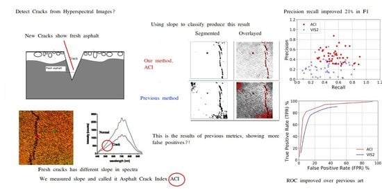
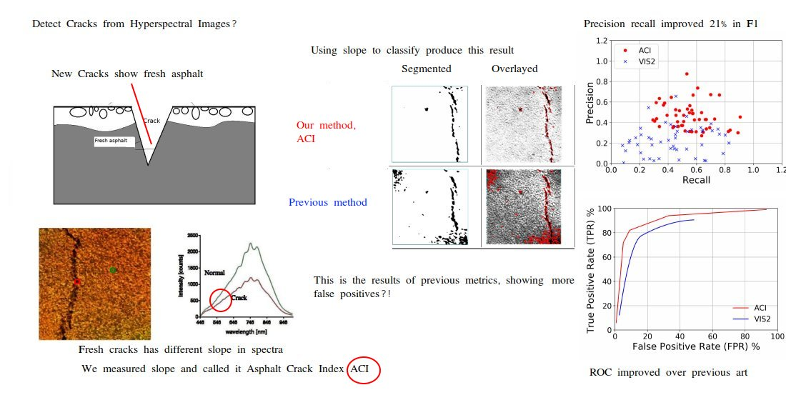
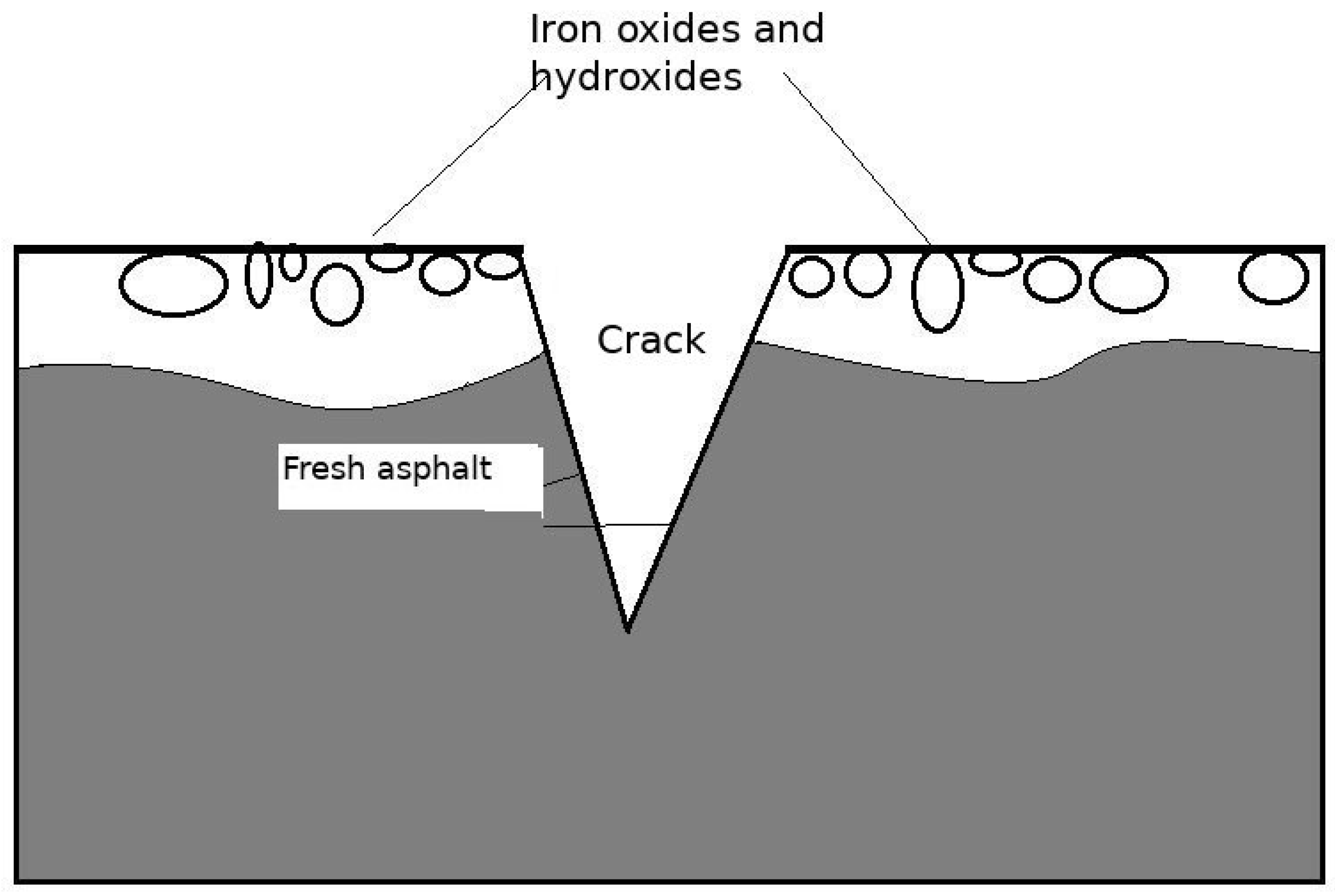
Roads are constantly subject to wear by vehicles’ tyres and therefore it has a brighter colour due to the partial appearance of aggregates used to build pavement layers and the wear of darker asphalt. Newly developed cracks will show up the road interior material, which is different from the pavement surface material. This difference in material can be easily detected by a hyper-spectral camera in a specific spectral band. The new crack shows darker material due to its asphalt content, which is rich in heavy hydrocarbons and oil. The darkening of cracks in images may also result due to the cavity shading as well and this will be illustrated in the experimental section. This condition acts as a strong physical clue to discriminate road cracks from other edges.

The regions used for pavement inspection are shown in Figure 2 showcasing the typical response curve from an HSC. It is known that the range of 450–900 nm is sensitive to the iron oxides and iron hydroxides [47]. The camera used is working in the Visible and Near Infra Red (VNIR) spectral range. That means the spectral range that can be of interest for road material change detection, and hence cracks, is the range similar to that used by VIS2 metric and showing metal and iron oxide in particular.

The response in the VNIR range changes significantly for road based on age and wear as reported in several studies (e.g., [6,11,12]). The hypothesis of this paper is that cracks show different material, and therefore, present a different spectral response. The main idea is explained schematically in Figure 3. The crack shows the internal pavement material, which is different from the road surface due to surface wear. The surface usually reflects bright light because of partial appearance of gravel pigments and loss of the bonding asphalt rich in hydrocarbon and oil.

In the previous work, only the intensity at two spectral bands was used to derive the VIS2 ratio. The new Asphalt Crack Index (ACI) relies on the observation from Figure 4, that the slope is different between cracks and normal surfaces in the range 450–550 nm. In this paper, the approximate line that represents the spectrum in the region between 450 and 550 nm is used. The slope angle, ${\varphi }_1$ is computed in the range 450–550 nm relative to the horizontal axis from the following equation:

$$ACI=\varphi =\arctan \left(\frac{I_{\lambda =550nm}-I_{\lambda =450nm}}{550.0-450.0}\right)$$

(3)

The reason for selecting the range (450–550 nm) is the observation of the slope in this region. The boundary of 450 nm is decided by the camera specification for the least spectral measurement and the upper boundary of 550 nm has been decided manually from observing the spectral response curves. The spectral range is a subset of the total iron oxide range 450–900 nm. There is an assumption that the surfaces are clean because the spectral response depends on the surface condition.

The rate of intensity darkening in this spectral zone is claimed to be an indication of material change rather than the shading effect and this will be proved experimentally. The ACI histogram is shown in Figure 5 for a sample crack image. The index can be represented in radians or degrees and its range is 0–1.571 rad or 0–90 degrees. The threshold value for the ACI is 1.53 rad and this has been identified manually and is confirmed to give best results.

The images are then classified according to the algorithm described in Algorithm 1. The process of computing is shown in Figure 6 indicating the input image, computed ACI and the thresholded image.

Algorithm 1: Pseudo-code for crack extraction from hyperspectral images.

4. Experiments

The objective of the experiments is to explore the ability of the ACI to detect cracks from HSI and quantify the performance compared with the VIS2 metric.

4.1. Conditions and Metrics

The full spectral range for hyperspectral imaging is 350–2500 nm, which extends beyond the human vision range (400–700 nm). The hyperspectral camera used in this study is a Cubert (model S185) measuring in the range 450–950 nm across 125 channels and fitted with a lens of 23 mm focal length.

Table 1. Summary of Hyperspectral Camera Specifications.

Category	Value
Focal length	23 mm
Wavelength range	450–950 nm
Spectral resolution	8 nm
Spectral sampling	4 nm 125 channels
Spatial resolution	1000 × 1000 pixels
Signal to Noise Ratio (SNR)	58 dB

shows a summary of hyperspectral camera specifications. The images were then processed and classified using the ENVI software package [49].

Experiments were made in the city of Leeds, northern areas in St. Helens lane and Adel wood grove, LS16 8JJ, UK, on the 20 April 2020 at 16:00, 25 June 2020 at 16:25 and 6 August at 16:00 in 2020, and the weather was mostly cloudy.

In the optical system used, one pixel represents (0.5 × 0.5) mm area at a one-metre distance. The spectral range of the camera enables the measurement of the iron oxides sensitive spectra as shown in Figure 2. Ground truth crack images were obtained by hand annotating the test images. The test images and results are available in supplementary material with this paper. Recall-precision analysis is used with the following definitions:

$$recall=\frac{TP}{TP+FN}$$

(4)

$$precision=\frac{TP}{TP+FP}$$

(5)

where TP is the True Positives, FN is the False Negatives and FP is the False Positives. The F1 score can be computed from both recall and precision using the following formula:

$$F1score=\frac{2·precision·recall}{precision+recall}$$

(6)

The Pratt Figure of Merit, PFOM, [50] can quantitatively measure the edge detection performance by considering the differences between a reference and a test subject; the reference subject is the step function in edge detection. It is defined by:

$$PFOM=\frac{1}{max(I_A,I_I)}\sum _{i=1}^{I_A}\frac{1}{1+d_i{a}^2}$$

(7)

where $i,I_A,I_I,d_i,a$ are respectively the edge pixel index, detected edges, the ideal edges, the distance between the actual and the ideal edges, and a design constant used to penalize displaced edges.

4.2. Separability

Several experiments were conducted using the camera to capture real crack images in paved roads and three sample images are shown in Figure 7. The location of cracks are known in these experiments and both ’normal surface’ and ’crack’ pixels were randomly selected from identified areas.

It is observed in Figure 7 of the spectral response that this particular region can be approximated by a straight line. This justification is proved empirically through the experiments.

The images are shown on the left-hand side of Figure 7 and two square windows marked in the image, one for normal road surface and another for a crack region. The right-hand side curve shows the spectral response of both normal surface and crack reflection. The area used to capture the spectrum is fixed during this experiment to one pixel size.

It can be observed in Figure 7, that the overall reflection on spectra from cracks is lower than in flat surfaces. It can also be observed that the slope of the spectrum in the 450–550 nm range is radically different from normal to crack surfaces. It can also be observed that the slope angle is lower for the crack regions than the surface regions of the pavements in most of the cases.

The VIS2 ratio was computed for the same sample set and is shown in Figure 8 as a ratio Equation (2). The VIS2 difference Equation (1) is also computed and shown in Figure 8.

The histograms of this angle computed for cracks and normal surfaces have very little overlap as shown in the right-hand side of Figure 8. However, for any given sample, the angle of slope of a crack is always lower than that of the road surface. This implies that a single threshold can be used to discriminate cracks from normal surfaces. It is observed that the histograms are almost 80% overlapping in Figure 8 for the VIS2 ratio and difference compared to less than 20% overlap for the proposed slope angle.

The experiment was made to check the ability of ACI to detect material changes not related to deep cracks and the results are summarised in Figure 9. The case A9 shows surface contours of fresh asphalt overlayed around a manhole, and the ACI can detect the material shown in the red colour area. The A15 case shows spots of recent asphalt on pavement, and it is easily detected by the ACI also shown in red colour. The ability to detect potholes of fresh asphalt content on the road is shown in case A17, where the pothole is detected in red. The case for A20 shows a pothole filled with fresh asphalt, and this is again detected and shown in red. The detection of fresh asphalt in these cases confirms that the ACI can detect material changes from fresh asphalt to slightly aged asphalt.

The ACI is measuring the rate at which asphalt is getting dark in a small spectral region. It is not measuring the asphalt darkness itself, which may be due to local shading across the crack depth. In some cases where the crack is old, the ACI did not detect any change of material since the exposed asphalt gets aged.

4.3. Comparisons

The crack images were classified using SAM and SFF methods, and the results are shown in Figure 10 and the reference sample was manually selected from the crack region. The output of the algorithms does not represent the crack shown on the right. The poor results because the spectral difference between cracks and road normal surface is not enough to trigger sufficient response. This is believed to be the reason behind the use of the VIS2 metric to classify road pavement conditions and grading it.

Hyperspectral images were classified based on the ACI, and are displayed in Figure 11 showing the classified image in the left column and overlayed on the original image in the right column. The first row shows the orginal image and the image of ACI on the right. The second row shows the classified image using the ACI computed in the range 450–500 nm with 50 nm difference only. The third row shows the result using the ACI computed from 450–550 nm with a 100 nm difference. The fourth row shows the result for the VIS2 metric. It can be observed that the VIS2 classification shows more false positive pixels than the real cracks shown on the original image. The result in the third row for 100 nm shows that the result is better than the 50 nm case in the second row in terms of increased recall and better precision.

Sample classified images are given in Figure 12, showing the original, ground truth, VIS2 and ACI-classified images. It is clear that the VIS2 results show more false positive pixels and the ACI on the right column is closer in performance to the ground truth images. This observation is quantified in Figure 13 showing a comparison of the F1 score for both the ACI and VIS2 and it shows that the F1 score is higher for the ACI in all cases.

Table 2. Comparison of VIS2 and ACI for 50 hyperspectral crack images captured on road pavement in Leeds city, UK.

Image No.	VIS2 Recall	VIS2 Precision	VIS2 F1 Score	VIS2 PFOM	ACI Recall	ACI Precision	ACI F1 Score	ACI PFOM
1	0.101	0.124	0.112	0.233	0.453	0.525	0.486	0.656
2	0.264	0.253	0.258	0.39	0.553	0.564	0.558	0.692
3	0.287	0.182	0.222	0.281	0.635	0.496	0.557	0.603
4	0.13	0.224	0.165	0.252	0.319	0.437	0.369	0.461
5	0.08	0.177	0.111	0.134	0.48	0.515	0.497	0.588
6	0.403	0.227	0.29	0.313	0.575	0.488	0.528	0.612
7	0.206	0.344	0.258	0.427	0.55	0.495	0.521	0.627
8	0.348	0.21	0.262	0.358	0.608	0.736	0.666	0.754
9	0.125	0.204	0.155	0.225	0.536	0.531	0.534	0.668
10	0.53	0.142	0.224	0.19	0.662	0.43	0.522	0.511
11	0.172	0.251	0.204	0.408	0.376	0.589	0.459	0.512
12	0.437	0.17	0.245	0.231	0.306	0.413	0.352	0.448
13	0.418	0.147	0.217	0.208	0.293	0.425	0.347	0.438
14	0.444	0.144	0.218	0.186	0.467	0.408	0.436	0.537
15	0.208	0.104	0.139	0.165	0.519	0.318	0.394	0.395
16	0.282	0.24	0.259	0.38	0.471	0.362	0.409	0.468
17	0.638	0.182	0.283	0.223	0.761	0.668	0.712	0.746
18	0.263	0.545	0.355	0.385	0.576	0.667	0.619	0.677
19	0.455	0.656	0.537	0.591	0.495	0.372	0.424	0.51
20	0.802	0.278	0.413	0.307	0.7	0.672	0.686	0.753
21	0.185	0.184	0.184	0.24	0.668	0.43	0.523	0.58
22	0.537	0.311	0.394	0.405	0.532	0.874	0.661	0.678
23	0.419	0.38	0.398	0.486	0.62	0.43	0.507	0.55
24	0.3	0.028	0.051	0.041	0.693	0.35	0.465	0.53
25	0.382	0.402	0.392	0.572	0.339	0.36	0.349	0.44
26	0.461	0.136	0.21	0.189	0.368	0.57	0.447	0.48
27	0.787	0.098	0.174	0.11	0.423	0.645	0.510	0.56
28	0.592	0.047	0.087	0.054	0.434	0.35	0.3875	0.43
29	0.665	0.028	0.054	0.033	0.501	0.37	0.425	0.48
30	0.088	0.008	0.016	0.01	0.393	0.47	0.428	0.52
31	0.271	0.046	0.078	0.055	0.439	0.36	0.395	0.47
32	0.336	0.047	0.084	0.055	0.456	0.47	0.462	0.51
33	0.655	0.03	0.058	0.034	0.339	0.634	0.441	0.494
34	0.228	0.043	0.072	0.056	0.317	0.594	0.413	0.486
35	0.477	0.035	0.066	0.048	0.51	0.47	0.489	0.53
36	0.21	0.281	0.241	0.266	0.907	0.454	0.605	0.463
37	0.71	0.32	0.44	0.37	0.51	0.41	0.46	0.507
38	0.452	0.249	0.321	0.302	0.727	0.434	0.544	0.485
39	0.645	0.326	0.433	0.369	0.585	0.425	0.492	0.512
40	0.453	0.361	0.402	0.439	0.669	0.338	0.449	0.377
41	0.53	0.46	0.49	0.56	0.567	0.52	0.54	0.62
42	0.452	0.283	0.348	0.352	0.554	0.313	0.4	0.373
43	0.64	0.312	0.42	0.346	0.597	0.31	0.408	0.36
44	0.56	0.33	0.415	0.39	0.647	0.308	0.417	0.339
45	0.464	0.315	0.375	0.355	0.636	0.271	0.38	0.313
46	0.761	0.287	0.417	0.316	0.891	0.3	0.449	0.313
47	0.751	0.336	0.465	0.373	0.824	0.312	0.453	0.329
48	0.702	0.388	0.499	0.426	0.836	0.326	0.469	0.349
49	0.63	0.351	0.451	0.397	0.567	0.31	0.401	0.345
50	0.828	0.199	0.321	0.214	0.572	0.488	0.526	0.55

shows the recall, precision and F1 score for 50 test images. It is clear that the ACI shows much better performance.

The results of precision-recall analysis are summarised in Figure 14, where each point in the graph represents the results of a single test image. Both the results of the ACI and VIS2 are included for comparison. The ACI outperforms the VIS2 metric classification. The two sets are not disjoint in this graph, but the previous table can be consulted for a case by case comparison showing that only in five images VIS2 outperformed the ACI in terms of the F1 score.

The statistics of the tested 50 test images are summarised in

Table 3. Summary of performance metrics for 50 hyperspectral images of road pavement cracks.

Descriptor	VIS2	ACI	Change
Recall %	43.54%	54.91%	+11.37%
Precision %	22.85%	46.00%	+23.15%
F1 score %	26.57%	47.94%	+21.37%

. It can be seen that the F1 score increased by 21.37%, which is a significant improvement. The precision-recall sensitivity to changes in the threshold value is shown in Figure 15 and Figure 16 for the ACI and VIS2, respectively, computed for a sample image and a similar trend was observed in other images. The F1 score has a peak at an optimum threshold, which is 1.53 rad (ACI) and 5000 for the VIS2 case. The effect of the threshold on the precision-recall analysis is also shown in Figure 17. It is clear that the ACI performs better than the VIS2.

5. Discussion

The idea of using spectral information as an added clue to detect cracks reliably proved to be effective compared to the existing method of VIS2 and the ACI helped in this detection process. The added clues helped to find road pavement cracks that are hard to find in visible spectrum imaging because of the ambiguity with background textures.

It is clear that the geometrical properties of cracks alone do not provide useful clues for crack detection, simply because cracks have no distinct shapes. The spectral domain here was exploited with the assumption that cracks are newly developed to show different distinguishable surfaces in the hyperspectral image. The main assumption is that crack surfaces are free from debris and dust and are at least slightly worn roads or older roads.

This means the method will work better in older roads where new cracks form. This is, however, precisely the kind of asset where finding these cracks is essential as early detection allows for a prompt fix that stops further deterioration that may result in costly reparation.

The results showed significant improvement in the precision of crack detection, which confirmed the concept of crack verification from the ACI. Spatial resolution affects the ability to detect thin cracks from a distance and in our experiments the camera was used at a close distance to the road (one metre). Thin cracks in our experiments refer to 5 pixels width or length (2.5 mm in our system) and it gets harder to detect any thinner/shorter cracks.

Camera optics can be modified to help detect cracks from aerial images with sufficient spatial resolution. Conventional spectral classification algorithms are not suited to detect the different grades of asphalt due to aging, since the differences are not spectrally significant. The ACI index improves on the concept of VIS2 through measuring the gradient of change of intensity with respect to wavelength.

The results of ACI showed an improvement over the VIS2 metric but the overall F1 score may still be not high enough for commercial application. The ACI may suffer false positives for surface stains of fresh asphalt. In the future we will aim to combine this method with other crack detection methods to serve as added clues for detection and for discriminating false positives.

VIS2 had been used previously to classify road pavement condition and reported to give good results, but it seems this metric was more suited for long-range imaging. The ACI here outperformed VIS2 for close range imaging and this should be of interest for inspection in low altitude drone scenarios. HSC are expensive, and it would be useful to make the utmost utilization of their data in the simplest way without sacrificing useful information. There should be a compromise between the exploitability of spectral data and simplicity, which may dictate using only a few spectral data or just a multispectral camera working in the spectral region of interest.

6. Conclusions

The potential of hyper-spectral imaging is exploited in this paper to discover cracks in road pavement. The basic measurement concept is that a newly developed crack shows the road interior, which has fresh asphalt content relative to the worn asphalt road surface. When cracks are observed with an HSC, the spectral reflection caused by different materials will be a good clue to detect cracks. A novel ACI index is proposed to indicate the change of material through a formula measuring the intensity change in the spectral region of 450–550 nm. The ACI is the slope angle of the spectral line in this region that utilizes more information from the spectral response than the previous VIS2 indicator.

The new technique had been tested with a hyperspectral camera in the field and was found effective, and the ACI is confirmed by experiment to outperform the VIS2 metric. The F1 score was increased using the ACI by 21.37% relative to the case of the VIS2 metric. Exploiting more spectral information is useful to improve the clues used to find material changes and hence associate this with cracks.

References

- Gavilan, M.; Balcones, D.; Marcos, O.; Llorca, D.; Sotelo, M.; Parra, I.; Ocana, M.; Aliseda, P.; Yarza, P.; Amirola, A. Adaptive Road Crack Detection System by Pavement Classification. Sensors 2011, 11, 9628–9657. [Google Scholar] [CrossRef]
- Aldea, E.; Le Hegarat-Mascle, S. Robust crack detection for unmanned aerial vehicles inspection in an a-contrario decision framework. J. Electron. Imaging 2015, 24. [Google Scholar] [CrossRef] [Green Version]
- Furness, G.; Barnes, S.; Wright, A. Crack detection on local roads, phase 2. In TRL Limited for Traffic Management Division; Department for Transport: London, UK, 2019. [Google Scholar]
- Wang, W.; Wang, M.; Li, H.; Zhao, H.; Wang, K.; He, C.; Wang, J.; Zheng, S.; Chen, J. Pavement crack image acquisition methods and crack extraction algorithms: A review. J. Traffic Transp. Eng. 2019, 6, 535–556. [Google Scholar] [CrossRef]
- Schnebele, E.; Tanyu, B.F.; Cervone, G.; Waters, N. Review of remote sensing methodologies for pavement management and assessment. Eur. Transp. Res. Rev. 2015, 7. [Google Scholar] [CrossRef] [Green Version]
- Mohammadi, M. Road Classification and Condition Determination Using Hyperspectral Imagery. Int. Arch. Photogramm. Remote Sens. 2012, 141–146. [Google Scholar] [CrossRef] [Green Version]
- Gomez, R.B. Hyperspectral imaging: A useful technology for transportation analysis. Opt. Eng. 2002, 41, 2137. [Google Scholar] [CrossRef]
- Herold, M.; Gardner, M.E.; Noronha, V.; Roberts, D.A. Spectrometry and hyperspectral remote sensing of urban road infrastructure. J. Space Commun. 2003, 3, 1–29. [Google Scholar] [CrossRef]
- Andreou, C.; Karathanassi, V.; Kolokoussis, P. Investigation of hyperspectral remote sensing for mapping asphalt road conditions. Int. J. Remote Sens. 2011, 32, 6315–6333. [Google Scholar] [CrossRef]
- Carmon, N.; Ben-Dor, E. Mapping asphaltic roads’ skid resistance using imaging spectroscopy. Remote Sens. 2018, 10, 430. [Google Scholar] [CrossRef] [Green Version]
- Herold, M.; Roberts, D.A. Spectral characteristics of asphalt road aging and deterioration: Implications for remote-sensing applications. Appl. Opt. 2005, 44, 4327–4334. [Google Scholar] [CrossRef]
- Noronha, V.; Herold, M.; Roberts, D.; Gardner, M. Spectrometry and Hyperspectral Remote Sensing for Road Centerline Extraction and Evaluation of Pavement Condition. In Proceedings of the Pecora Conference, San Diego, CA, USA, 11–13 March 2002. [Google Scholar]
- Liang, J. Spectral-spatial Feature Extraction for Hyperspectral Image Classification. Ph.D. Thesis, College of Engineering and Computer Science, The Australian National University, Canberra, Australia, 2016. [Google Scholar]
- Jengo, C.; Laveigne, J.; Curtis, I. Pothole Detection and Road Condition Assessment Using Hyperspectral Imagery. In Proceedings of the American Society for Photogrammetry & Remote Sensing (ASPRS) 2005 Annual Conference, Baltimore, MD, USA, 7–11 March 2005. [Google Scholar]
- Herold, M.; A., R.D.; Smadi, O.; Noronha, V. Road Condition Mapping with Hyperspectral Remote Sensing. In JPL Airborne Earth Science Workshop; JPL Publication: Pasadena, CA, USA, 2004. [Google Scholar]
- Pan, Y.; Zhang, X.; Cervone, G.; Yang, L. Detection of Asphalt Pavement Potholes and Cracks Based on the Unmanned Aerial Vehicle Multispectral Imagery. IEEE J. Sel. Top. Appl. Earth Obs. Remote Sens. 2018, 11, 3701–3712. [Google Scholar] [CrossRef]
- Herold, M.; Roberts, D.; Noronha, V.; Smadi, O. Imaging spectrometry and asphalt road surveys. Transp. Res. Part Emerg. Technol. 2008, 16, 153–166. [Google Scholar] [CrossRef]
- Abdellatif, M.; Peel, H.; Cohn, A.; Fuentes, R. Hyperspectral Imaging for Autonomous Inspection of Road Pavement Defects. In Proceedings of the 36th International Symposium on Automation and Robotics in Construction (ISARC), Banff, AB, Canada, 21–24 May 2019; pp. 384–392. [Google Scholar]
- Adao, T.; Hruska, J.; Padua, L.; Bessa, J.; Peres, E.; Morais, R.; Sousa, J. Hyperspectral Imaging: A Review on UAV-Based Sensors, Data Processing and Applications for Agriculture and Forestry. Remote Sens. 2017, 9, 1110. [Google Scholar] [CrossRef] [Green Version]
- Tsouvaltsidis, C.; Zaid Al Salem, N.; Benari, G.; Vrekalic, D.; Quine, B. Remote Spectral Imaging Using A Low Cost UAV System. Int. Arch. Photogramm. Remote Sens. Spat. Inf. Sci. 2015. [Google Scholar] [CrossRef] [Green Version]
- Polak, A.; Kelman, T.; Murray, P.; Marshall, S.; Stothard, D.; David, J.; Eastaugh, N.; Eastaugh, F. Hyperspectral imaging combined with data classification techniques as an aid for artwork authentication. Cult. Herit. 2017, 26, 1–11. [Google Scholar] [CrossRef]
- Deborah, H.; Richard, N.; Hardeberg, J. Hyperspectral crack detection in paintings. In Proceedings of the 2015 Colour and Visual Computing Symposium (CVCS), Gjovik, Norway, 25–26 August 2015; pp. 1–6. [Google Scholar]
- Li, F.; NG, M.; Plemmons, R.; Prasad, S.; Zhang, Q. Hyperspectral image segmentation, deblurring, and spectral analysis for material identification. In Proceedings of the SPIE-Defense-Commercial-Sensing, Visual Information Processing, Orlando, FL, USA, 6–7 April 2010. [Google Scholar]
- Kruse, F.; Lefkoff, A.; Boardman, J.; Heidebrecht, K.; Shapiro, A.; Barloon, P.; Goetz, A. The spectral image processing system (SIPS)—Interactive visualization and analysis of imaging spectrometer data. Remote Sens. Environ. 1993, 44, 145–163. [Google Scholar] [CrossRef]
- Robila, S.; Gershman, A. Spectral Matching Accuracy in Processing Hyperspectral Data. In Proceedings of the IEEE International Symposium on Signals, Circuits and Systems, Iasi, Romania, 14–15 July 2005; pp. 163–166. [Google Scholar]
- Robila, S.A. An Investigation of Spectral Metrics in Hyperspectral Image Preprocessing for Classification. In Proceedings of the Annual Conference 2005-Geospatial Goes Global: From Your Neighborhood to the Whole Planet, Baltimore, MD, USA, 7–11 March 2005; pp. 942–951. [Google Scholar]
- Bertels, L.; Bart, D.; Pieter, K.; Walter, D.; Sam, P. Optimized Spectral Angle Mapper Classification of Spatially Heterogeneous Dynamic Dune Vegetation, a Case Study Along the Belgian. In Proceedings of the 9th International Symposium on Physical Measurements and Signatures in Remote Sensing (ISPMSRS), Beijing, China, 17–19 October 2005; pp. 1–6. [Google Scholar]
- Li, H.; Lee, W.S.; Wang, K.; Ehsani, R.; Yang, C. Extended Spectral Angle Mapping (ESAM) for Citrus Greening Disease Detection Using Airborne Hyperspectral Imaging. Precis. Agric. 2014, 15, 162–183. [Google Scholar] [CrossRef]
- Chang, C.I. An Information-Theoretic Approach to Spectral Variability, Similarity, and Discrimination for Hyperspectral Image Analysis. IEEE Trans. Inf. Theory 2000, 46, 1927–1932. [Google Scholar] [CrossRef] [Green Version]
- Du, Y.; Chang, C.I.; Ren, H.; Chang, C.C.; Jensen, J.O.; D’Amico, F.M. New Hyperspectral Discrimination Measure for Spectral Characterization. Opt. Eng. 2004, 43, 1777–1786. [Google Scholar] [CrossRef] [Green Version]
- Wang, K.; Yong, B. Application of the Frequency Spectrum to Spectral Similarity Measures. Remote Sens. 2016, 8, 344. [Google Scholar] [CrossRef] [Green Version]
- Khuwuthyakorn, P.; Robles-Kelly, A.; Zhou, J. Affine Invariant Hyperspectral Image Descriptors Based upon Harmonic Analysis. In Machine Vision Beyond Visible Spectrum; Springer: Berlin/Heidelberg, Germany, 2011; pp. 179–199. [Google Scholar]
- Gao, Q.; Lim, S.; Jia, X. Hyperspectral Image Classification Using Convolutional Neural Networks and Multiple Feature Learning. Remote Sens. 2018, 10, 299. [Google Scholar] [CrossRef] [Green Version]
- Liu, P.; Zhang, H.; Eom, K. Active Deep Learning for Classification of Hyperspectral Images. IEEE J. Sel. Top. Appl. Earth Obs. Remote Sens. 2017, 10, 712–724. [Google Scholar] [CrossRef] [Green Version]
- Fauvel, M.; Chanussot, J.; Benediktson, J.A.; Sveinson, J.R. Spectral and Spatial Classification of Hyperspectral Data Using SVMs and Morphological Profiles. IEEE Geosci. Remote Sens. 2008, 46, 4834–4837. [Google Scholar] [CrossRef] [Green Version]
- Zhao, W.; Du, S.; Emery, W.J. Object-Based Convolutional Neural Network for High-Resolution. IEEE J. Sel. Top. Appl. Earth Obs. Remote Sens. 2017, 10, 3386–3396. [Google Scholar] [CrossRef]
- Plaza, J.; Plaza, A.; Perez, R.; Martinez, P. On the use of small training sets for neural network-based characterization of mixed pixels in remotely sensed hyperspectral images. Pattern Recognit. 2009, 42, 3032–3045. [Google Scholar] [CrossRef]
- Lin, Z.; Chen, Y.; Zhao, X.; Wang, G. Spectral-Spatial Classification of Hyperspectral Image Using Autoencoders. In Proceedings of the 2013 9th International Conference on Information, Communications & Signal Processing, Tainan, Taiwan, 10–13 December 2013. [Google Scholar]
- Xing, C.; Ma, L.; Yang, X. Stacked Denoise Autoencoder Based Feature Extraction and Classification for Hyperspectral Images. J. Sens. 2016, 1–10. [Google Scholar] [CrossRef] [Green Version]
- Chen, Y.; Lin, Z.; Zhao, X.; Wang, G.; Gu, Y. Deep Learning-Based Classification of Hyperspectral Data. IEEE J. Sel. Top. Appl. Earth Obs. Remote Sens. 2014, 7, 2094–2107. [Google Scholar] [CrossRef]
- Zhao, W.; Du, S. Spectral Spatial Feature Extraction for Hyperspectral Image Classification: A Dimension Reduction and Deep Learning Approach. IEEE Trans. Geosci. Remote Sens. 2016, 54, 4544–4554. [Google Scholar] [CrossRef]
- Jia, X.; Kuo, B.; Crawford, M. Feature Mining for Hyperspectral Image Classification. Proc. IEEE 2013, 101, 676–697. [Google Scholar] [CrossRef]
- Kong, X.; Zhao, Y.; Xue, J.; Chan, J.C.W.; Kong, S.G. Global and Local Tensor Sparse Approximation Models for Hyperspectral Image Destriping. Remote Sens. 2020, 12, 704. [Google Scholar] [CrossRef] [Green Version]
- Cazzato, D.; Cimarelli, C.; Sanchez-Lopez, J.L.; Voos, H.; Leo, M. A Survey of Computer Vision Methods for 2D Object Detection from Unmanned Aerial Vehicles. J. Imaging 2020, 6, 78. [Google Scholar] [CrossRef]
- Mettas, C.; Themistocleous, K.; Neocleous, K.; Christofe, A.; Pilakoutas, K.; Hadjimitsis, D. Monitoring asphalt pavement damages using remote sensing techniques. In Proceedings of the Third International Conference on Remote Sensing and Geoinformation of the Environment, Paphos, Cyprus, 16–19 March 2015. [Google Scholar]
- Lanaras, C.; Baltsavias, E.; Schindler, K. Hyperspectral super-resolution with spectral unmixing constraints. Remote Sens. 2017, 9, 1196. [Google Scholar] [CrossRef] [Green Version]
- Clark, R. Spectroscopy of Rocks and Minerals, and Principles of Spectroscopy. Man. Remote Sens. 1999, 3, 2. [Google Scholar]
- Ming-Hsiang, T. Geographic Information Science and Spatial Reasoning Course, GIS Data Collection and Database Management Unit 6.1. 2018. Available online: https://map.sdsu.edu/geog104/unit-6.html (accessed on 14 September 2020).
- Software for Hyperspectral Image Processing, E. L3HARRIS, 2020. Available online: https://www.l3harrisgeospatial.com/Software-Technology/ENVI (accessed on 14 September 2020).
- Pratt, W.K. Digital Image Processing: PIKS Inside, 3rd ed.; John Wiley & Sons, Inc.: New York, NY, USA, 2001. [Google Scholar]
Figure 1.
Taxonomy of hyperspectral imaging (HSI) segmentation/classification approaches.
Figure 2.
Spectral response and regions for describing pavements [48].
Figure 3.
Schematic diagram showing the cross sectional view in a road pavement crack.
Figure 4.
Method of computing the angle (ACI) from the spectral response.
Figure 5.
Histogram of ACI for a sample crack image.
Figure 6.
The HSI processing.
Figure 7.
Sample hyperspectral images of pavements (left) and their spectral characteristics (right) inside the regions marked by coloured squares in the images. The upper line refers to the coloured pixel in the road surface and the lower curve represents the spectra of the pixel inside a crack area.
Figure 8.
Comparison for VIS2 metrics and ACI computed for sample pavement for crack and surface regions and the corresponding histograms.
Figure 9.
Sample images showing the change of asphalt material A9 and A15, and example for pothole detection A17 and A20.
Figure 10.
The results of Spectral Angle Mapper (SAM) and Spectral Feature Fitting (SFF) processing.
Figure 11.
Sample images showing ACI and VIS2 classification.
Figure 12.
Comparison between VIS2 and ACI for sample images.
Figure 13.
Comparison of F1 score computed for VIS2 and ACI to detect cracks from sample hyperspectral crack images.
Figure 14.
The precision-recall comparison between the VIS2 (blue crosses) and the ACI (red dots) in 50 HSI crack images.
Figure 15.
Effect of threshold value using ACI.
Figure 16.
Effect of threshold value using VIS2.
Figure 17.
ROC graph for both ACI and VIS2.