Comparison of Measured Surface Currents from High Frequency (HF) and X-Band Radar in a Marine Protected Coastal Area of the Ligurian Sea: Toward an Integrated Monitoring System

Abstract

Two different ground-based remote sensing instruments can be used for the near-real-time monitoring of surface waves and currents, namely the high frequency HF radar and the microwave X-band radar. The HF system reaches larger offshore distances at lower spatial resolutions and provides a poorer measurement of the wave-induced currents in very shallow waters. On the other hand, the X-band system achieves significantly higher spatial resolutions with a smaller offshore coverage. This study provides a preliminary comparison of the measured surface currents, obtained by the two different tools where they overlap. The comparison showed a good agreement between the measures with some discrepancies ascribable to the difference in the characteristics of the two radar technologies.

1. Introduction

The observation and monitoring of marine coastal currents is an important task for coastal protection, erosion control, and flood mitigation as well as near-shore fishing management and marine operations such as installations of offshore wind farms or oil and gas plants [1].

In recent years, the monitoring of surface currents with remote sensing techniques has greatly improved, making it possible to even perform real-time observations over sea surface areas of different extension. Among these techniques, two different ground-based remote sensing instruments can be deployed for the near-real-time monitoring of surface waves and currents, namely the high frequency HF radar and the microwave X-band radar. They directly measure the directional wave spectra at a spatial resolution from 250 m to 15 km, which depends on the specific allocated bandwidth and antenna design.

The overall spatial coverage of these tools significantly differs, as well does their spatial resolution. The HF system reaches larger offshore distances at lower spatial resolutions and provides a poorer measurement of the wave-induced currents in very shallow waters. On the other hand, the X-band system achieves significantly higher spatial resolutions with a smaller offshore coverage. The inherent differences of HF and X-band radars open new routes toward an integrated monitoring technique, which exploits the complementary nature of the output provided separately by the two systems [2,3].

High frequency (HF) coastal radars are very powerful instruments, providing information on surface velocity in terms of hourly maps over extended regions (range up to 100 km) and with high spatial resolution (order of 1–3 km). This information can be used to address several societal needs such as navigation safety, search and rescue, oil spill or other pollutant tracking, marine protected areas and fishery management [4,5].

The X-band radar represents a practical remote sensing system for sea waves and current monitoring in coastal and shallow waters. It is used for the acquisition and the analysis of consecutive sea surface images [6,7]. The surface current is retrieved from a sequence of these radar images by an inversion procedure, that accounts for the modulation effects that depend on both the sea state and the radar parameters as well as on the acquisition geometry [7,8,9,10,11].

This work is devoted to explore whether an integrated monitoring system can be successfully employed to measure surface currents in near real time across a variety of spatial scales. By blending HF and X-band radar data such an integrated system aims at reaching a high near-shore spatial resolution still covering a large off-shore area. This study provides a preliminary comparison of the measured surface currents, obtained by the two different tools where they overlap. Measurements taken at a selected study site located in the Ligurian Sea were analyzed.

As the present work focused on comparing two different measuring tools, rather than to study the local marine dynamics, an analysis of the surface circulation of the Ligurian Sea was beyond our aim and is already quite a well-covered topic in literature [12].

2. Materials and Methods

2.1. Study Site and Analyzed Sea Conditions

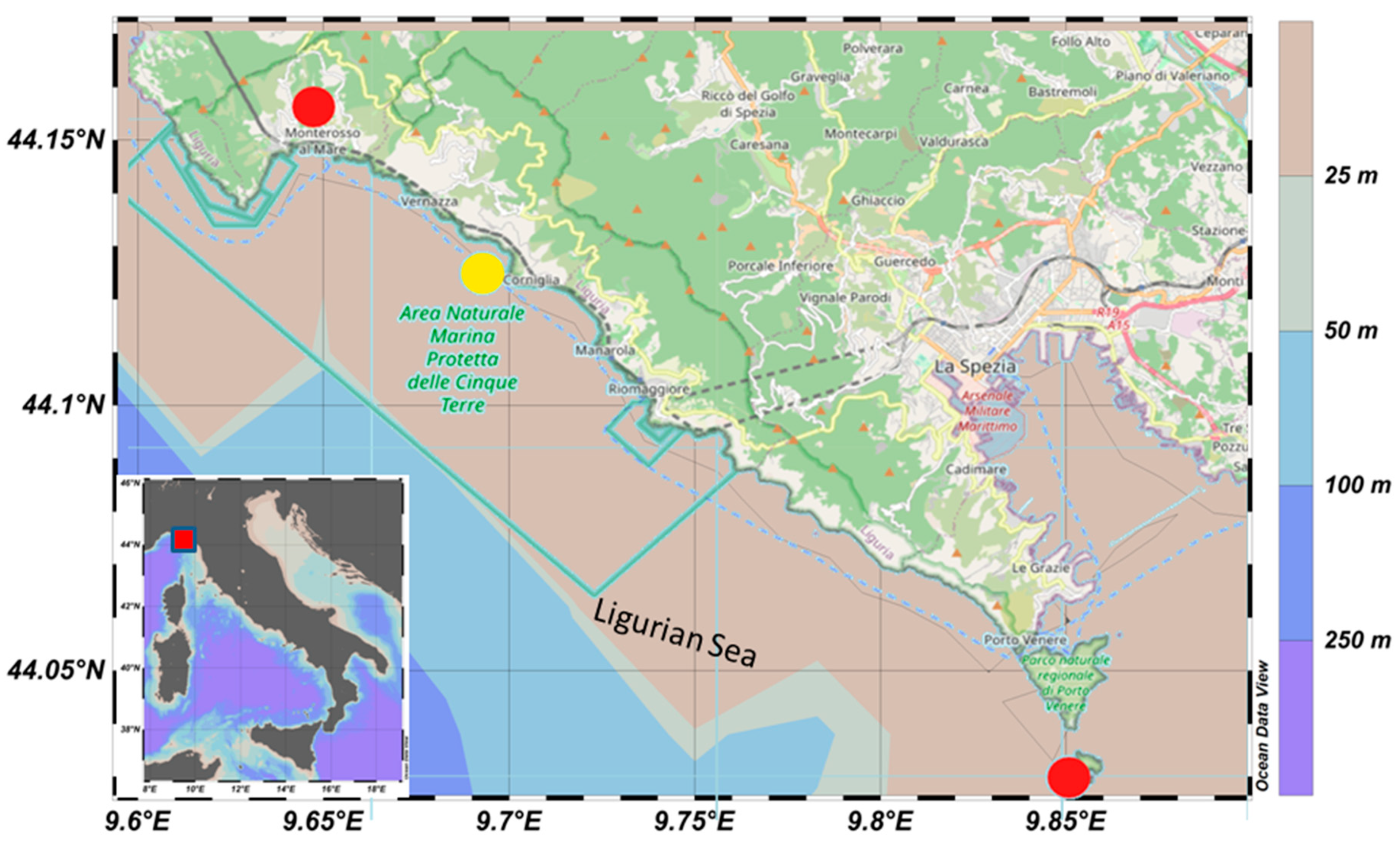
The study site is located within the Eastern Ligurian Sea, in the North West Mediterranean Sea as depicted in Figure 1, along a 15 km-long coastline in an area situated in front of which bounds an important Marine Protected Area (Cinque Terre).

A CNR-ISMAR HF Radar Network has been installed along the coast of Eastern Liguria, near La Spezia and Cinque Terre, in year 2016 and is composed by two CODAR SeaSonde HF radar stations operating in the frequency band of 25 MHz. A CONSILIUM/SELESMAR X-band radar was installed at Corniglia (SP) about 60 meters above sea level. The radar locations are shown in Figure 1.

At the installation site, the HF radar and the X-band radar both worked from 12 September 2017 to 1 April 2018.

The analysis was carried out as follows:

- As a first preliminary step, a qualitative snapshot comparison of the spatially-varying time-averaged surface velocity fields (horizontal components) derived by HF and X-Band is shown as a time average over a reduced time range. Despite this part has no quantitative aims, it allows us to show the overlapping points of the two instruments. Due to the different spatial resolutions involved, a linear interpolation in space was carried out to have measurements on matching grids. HF outputs were evaluated on the X-Band grid before qualitative comparison of the surface velocity time averaged field. However, due to the small overlap among them, only a few HF grid points resided within the X-Band grid. This likely makes the interpolated HF field oversmoothed, and a significant quantitative comparison at these scales is therefore not significant.

- A quantitative comparison at overlapping points was carried out for the measured time-series sampled from 12 September 2017 to 1 April 2018. The overlapping points between the HF and X-band grids, without any spatial interpolation, were identified and selected as comparison sites, namely A and B. The time-varying zonal (U) and meridional (V) surface velocity components, independently derived by the HF and X-band, were analyzed and compared at these locations. A comparison between the HF and X-Band time signatures, means, and standard deviations is given. Root mean square errors between X-band velocities and HF velocities at A and B were also computed.

2.2. HF Radar Data Collection and Analysis

The HF radar network was designed, implemented, and managed through the efforts of Institute of Marine Sciences - National Research Council (ISMAR-CNR La Spezia) [13]. HF radar data were collected and processed by ISMAR-CNR within the Ritmare and Jerico–Next projects [14]. The datasets hereinafter considered were downloaded from the website http://ritmare.artov.isac.cnr.it/thredds/catalog.html. Depending on the sea state, estimated errors ranged from 3 to 10 cm·s⁻¹ and explained only part of the rms difference of 10–20 cm·s⁻¹ found between HF and the in situ current measurements. The rest was assumed to be due the differences of the quantities measured (e.g., the spatial averaging [15]).

The acquisition settings are listed in

Table 1. HF Radar system parameters.

Frequency Band	Radial Coverage	Radial Range Cutoff	Radial Resolution	Angular Resolution
(MHz)	(km)	(km)	(km)	(deg)
26	35–45	45	1	5

.

HF radar is appropriate to detect surface ocean currents due to the diffraction grating effects of the rough sea surface [16,17]. Just when the radar signal scatters off a wave that is exactly half the transmitted signal wavelength, and that wave is traveling in a radial path either directly away from or toward the radar, the radar signal will return directly to its source. The scattered radar electromagnetic waves coherently add up, resulting in a strong energy return at a certain specific wavelength. The returning signal exhibits a Doppler-frequency shift that would always turn up at a known position in the frequency spectrum in the absence of ocean currents. Nevertheless, the observed Doppler-frequency shift does not match up exactly with the theoretical wave speed. The Doppler-frequency shift includes the information of the principal ocean current on the wave velocity in a radial pathway, jointly with the theoretical wave speed. Total velocities are derived using least square fit, which maps radial velocities measured from individual sites on a Cartesian grid. The final result is a map of the horizontal components of the ocean currents, on a regular grid, in the area covered by two or more radar stations [14].

2.3. X-Band Radar Data Collection and Analysis

A CONSILIUM SELESMAR marine X-band radar was installed on the roof of the sewage treatment plant at Corniglia (SP) about 60 meters above sea level. The radar antenna was located at the coordinates 44°07′10″ N, 9°42′20″ E.

The radar system radiates a maximum power of 25 KW, operates in the short pulse mode (i.e., pulse duration of about 90 ns), and is equipped with an 9-ft (2.7 m) long antenna with horizontal polarization (HH). These features enable reaching a spatial resolution of about 9m and an angular resolution of approximately 0.9°. The signal received by the antenna was converted through an analog–digital converter and interpolated on a Cartesian grid with a regular spacing of about 10 m to obtain two-dimensional (2D) sea surface images. The image sequence acquired by the X-band radar was stored and processed, and each raw data sequence consisted of 64 individual images stored every 2.4 s. The accuracy of the X-band radar in terms of measured velocities was of the order 10 cm s⁻¹ [18].

The acquisition settings are listed in

Table 2. X-band radar system parameters.

Frequency Band	Radial Coverage	Time Range	Spatial Resolution	Angular Resolution
(MHz)	(km)	(s)	(m)	(deg)
9200	5.55	2.4	9	0.9

.

The image processing to extract the inhomogeneous surface current fields from the X-band radar data were based on the so called “Local Method”, proposed in [19,20] and can be applied to data acquired in coastal areas, where the presence of coastlines and varying bathymetry cause a spatial inhomogeneity of the wave motion [3,21,22,23].

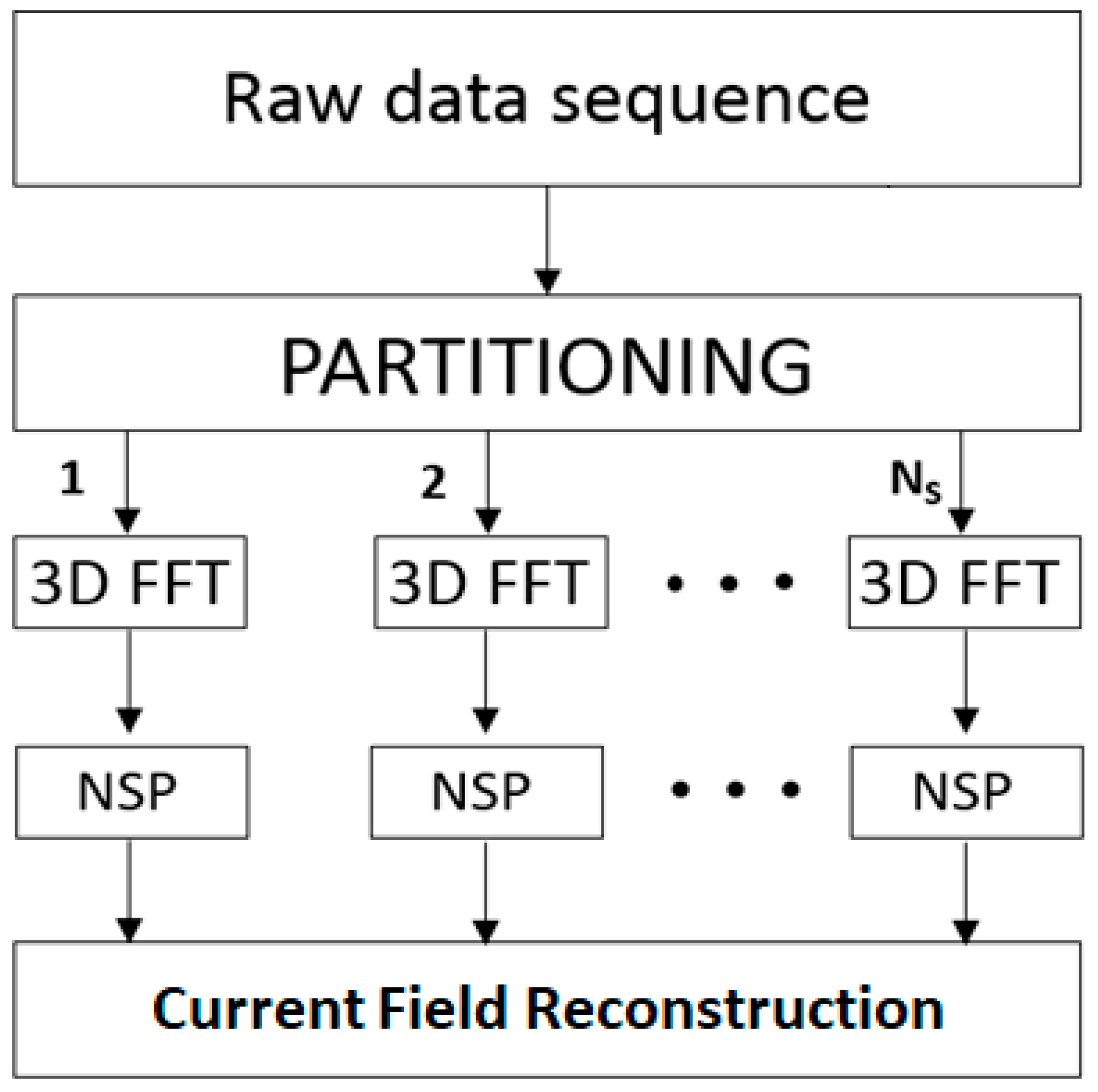
A block diagram of the inversion procedure is presented in Figure 2.

The partitioning procedure is needed to extract N_s spatially overlapping sub-areas, so it is possible to assume the waves’ homogeneity and uniformity from the analyzed radar data temporal sequence. After that, the fast Fourier transform (FFT) is applied to the N_s temporal sub-sequences to obtain the 3D radar sub-spectra.

Each spectrum is expressed as ${\left\{F^j\left(\acute{k},\omega \right)\right\}}_{j=1,\dots ,N_s}$, where $\acute{k}=\left(k_x,k_y\right)$ is the wave-number vectorand $\omega$ the angular frequency; spectra are then analyzedby applying the normalized scalar product (NSP) technique [7], in order to retrieve the local surface current vector through the following estimator:

$$V^j\left(\acute{U}\right)=arg\underset{h}{max}\frac{\langle \left|F^j\left(\acute{k},\omega \right)\right|,G\left(\acute{k},\omega ,\acute{U}\right)\rangle }{\sqrt{P_F{P}_G}}$$

(1)

where $G\left(\acute{k},\omega ,\acute{U}\right)=\delta \left(\omega -\sqrt{gk}-\acute{k}·\acute{U}\right)$ is the characteristic function based on the dispersion relation; $\delta (·)$ is the Dirac delta distribution;$\langle \left|F\right|,G\rangle$ represents the scalar product between the functions $\left|F\right|$ and $G$; and $P_F$ and $P_G$ are the powers associated with $\left|F\right|$ and $G$, respectively.

Once the local (sub-areas) current vectors have been estimated, it is possible to define the ‘global’ (applied to the whole radar spectrum) band-pass (BP) filter [3,20,21].

3. Results and Discussion

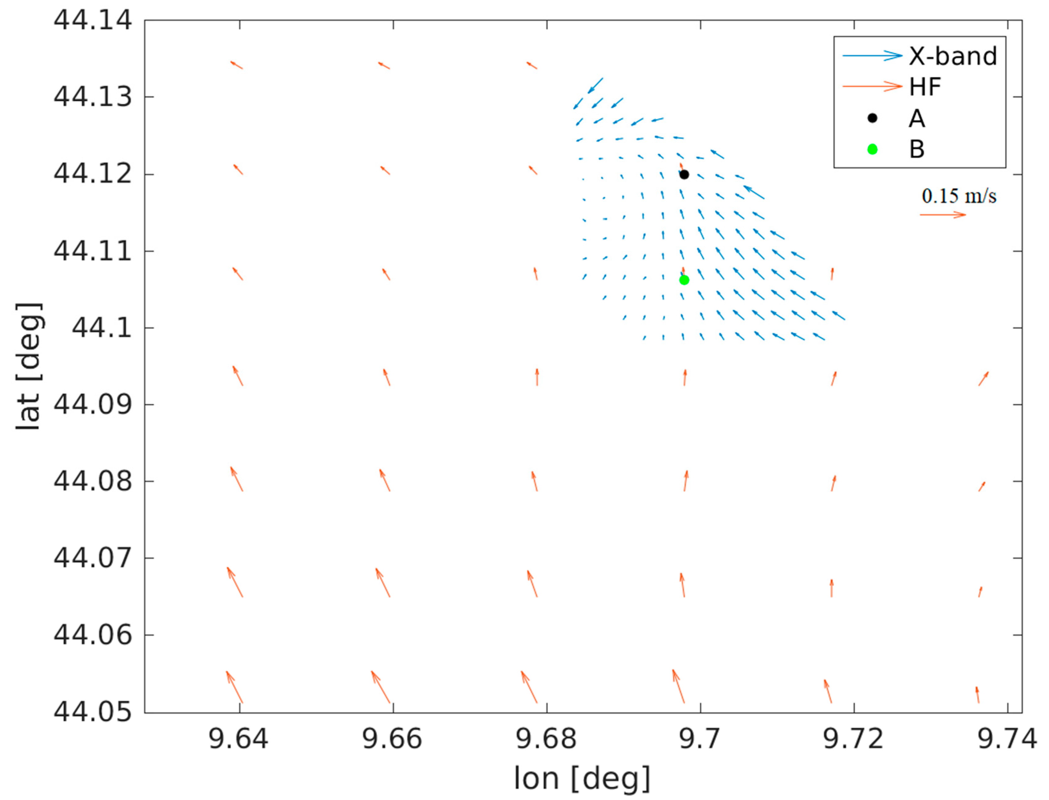
Figure 3 shows a qualitative snapshot of the HF and X-band surface velocity fields, time averaged over a sample period on the original spatial grids, with the purpose to qualitatively show the coverage overlaps and the overlapping points. More in detail, red (blue) arrows are located at the HF (X-band) grid points, whereas colored dots indicate the instruments overlaps.

Due to the very different spatial resolutions, some differences in the spatial velocity patterns may arise between the HF and X-band, which capture different spatial scales. Strong spatial variability at the HF sub-grid level may not be completely captured by the low resolution radar, resulting in an over-smoothed surface circulation, especially in the coastal zone. In order to cover coastal waters with HF measurements at a higher spatial resolution, a rather trivial option is to linearly interpolate the HF-derived currents on a finer grid to compensate for the missing locations. However, it of course does not improve the quality of data, as the sub-grid processes still remain unresolved. Although the main large-scale current direction is consistently measured by the two instruments, the HF-derived circulation pattern does not capture the details of the near-shore spatial variability, especially in the west–northwest portion of the domain. Here, the X-band measurements revealed the existence of a cyclonic branch at the western edge of the grid, which was instead missed by the HF-derived data at the same location.

As clearly visible in Figure 3, at intermediate off-shore distances, an overlapping zone exists between the HF and X-band grids, where the time-series of surface velocities can be directly compared without any additional interpolation in space. In such an intermediate zone, X-band and HF derived data without spatial interpolation are expected to give similar results over time if the X-band surface currents are correctly derived. Seaward of these overlapping locations, the HF radar has the advantage of a long distance coverage suitable to capture larger scale circulation structures, whereas the X-band becomes advantageous shoreward of the overlapping areas, where smaller scale dynamics needs to be resolved.

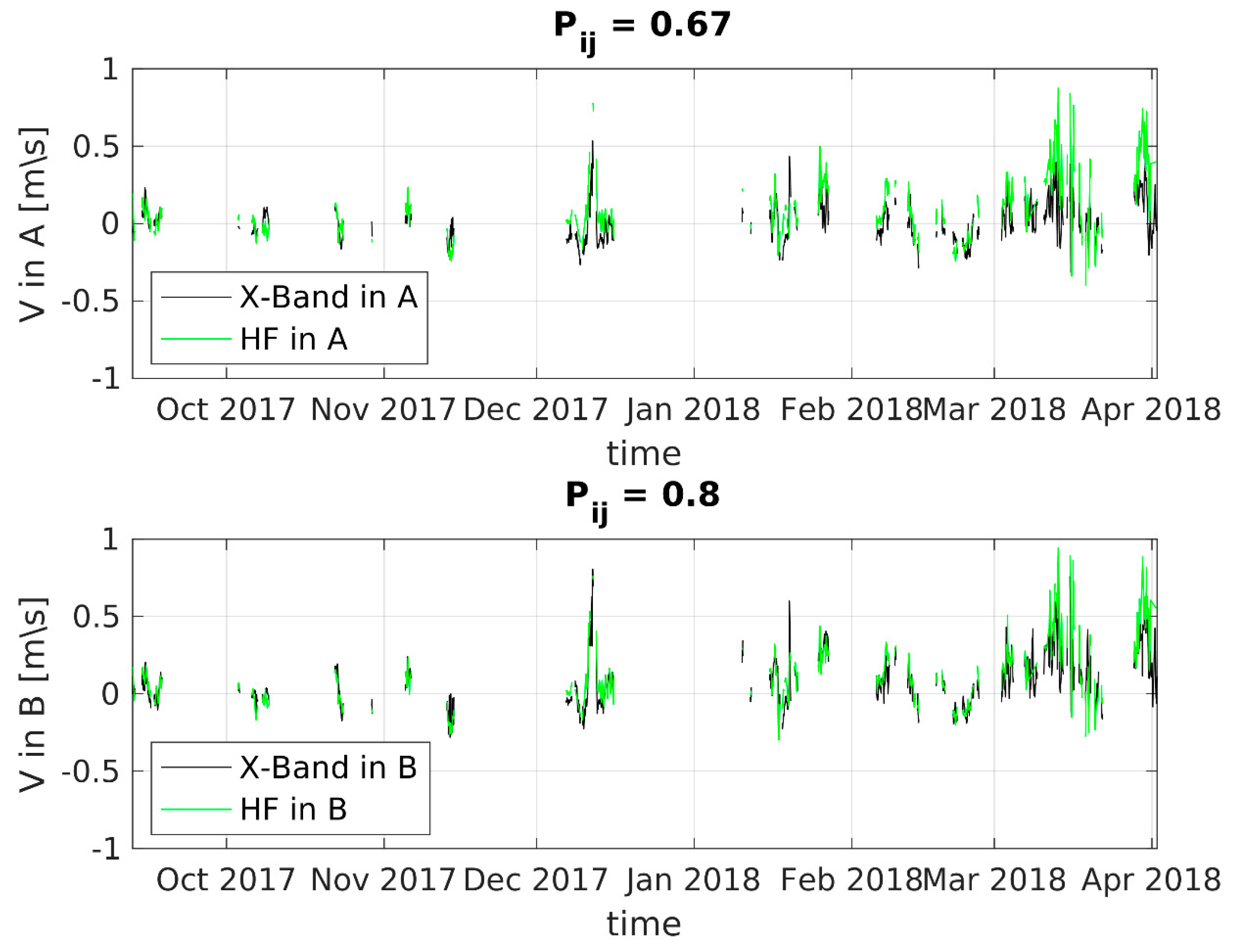
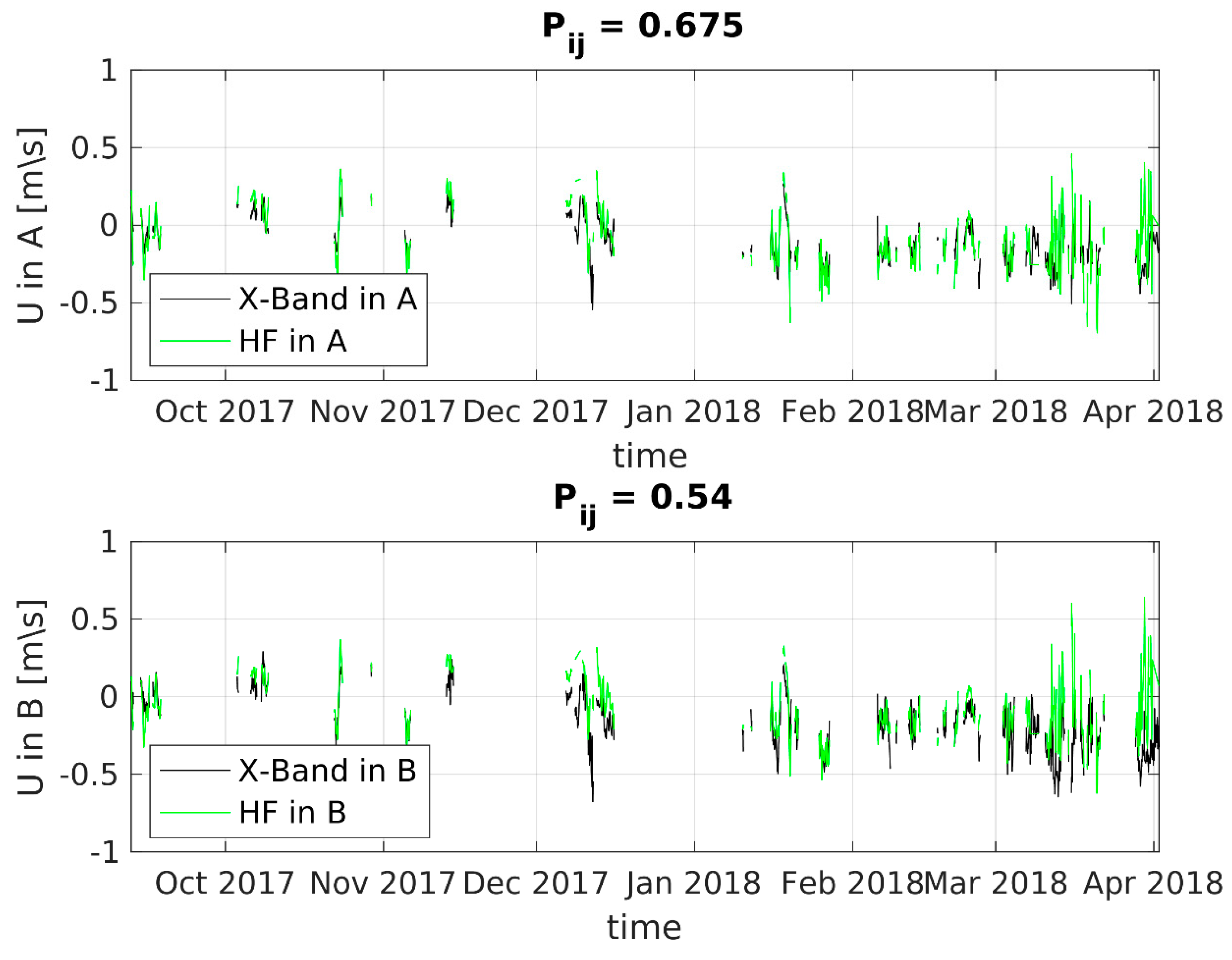
Time series of the northward and eastward surface velocity components, derived by HF and X-band radar at overlapping points A and B, are reported in Figure 4 and Figure 5, respectively, from 12 September 2017 to 1 April 2018. In each panel of Figure 4 and Figure 5, the green line refers to the HF measurements, whereas the black line shows the X-band ones. Missing data in the time series corresponds to periods where the X-band radar system did not work or the surface dynamics in the near shore area, covered by the X-band radar, cannot be measured with enough accuracy due to low sea state or rain that affect the current field estimation.

HF derived currents are provided as hourly means, whereas X-band measurements are obtained as instantaneous values at irregular time steps (multiple time steps per hour). In order to get a clearer comparison, the X-band data were therefore averaged over time to get hourly means. The HF values were then linearly interpolated in time in order to match the X-band hourly mean time spacing.

X-band derived velocity components display a good agreement with the HF counterpart throughout the sampling. A significant (p value << 0.01) positive correlation among the data was also indicated by the Pearson’s linear correlation coefficients Pij, here computed. Pij was 0.675 and 0.54 for the U components in A and B, respectively, whereas it had a value of 0.67 and 0.8 for V in A and B, respectively. The root mean square errors of U at point A and B were 0.14 m/s 0.17 m/s, respectively, while for the northward components, it assumed the values of 0.14 m/s and 0.13 m/s in A and B, respectively. 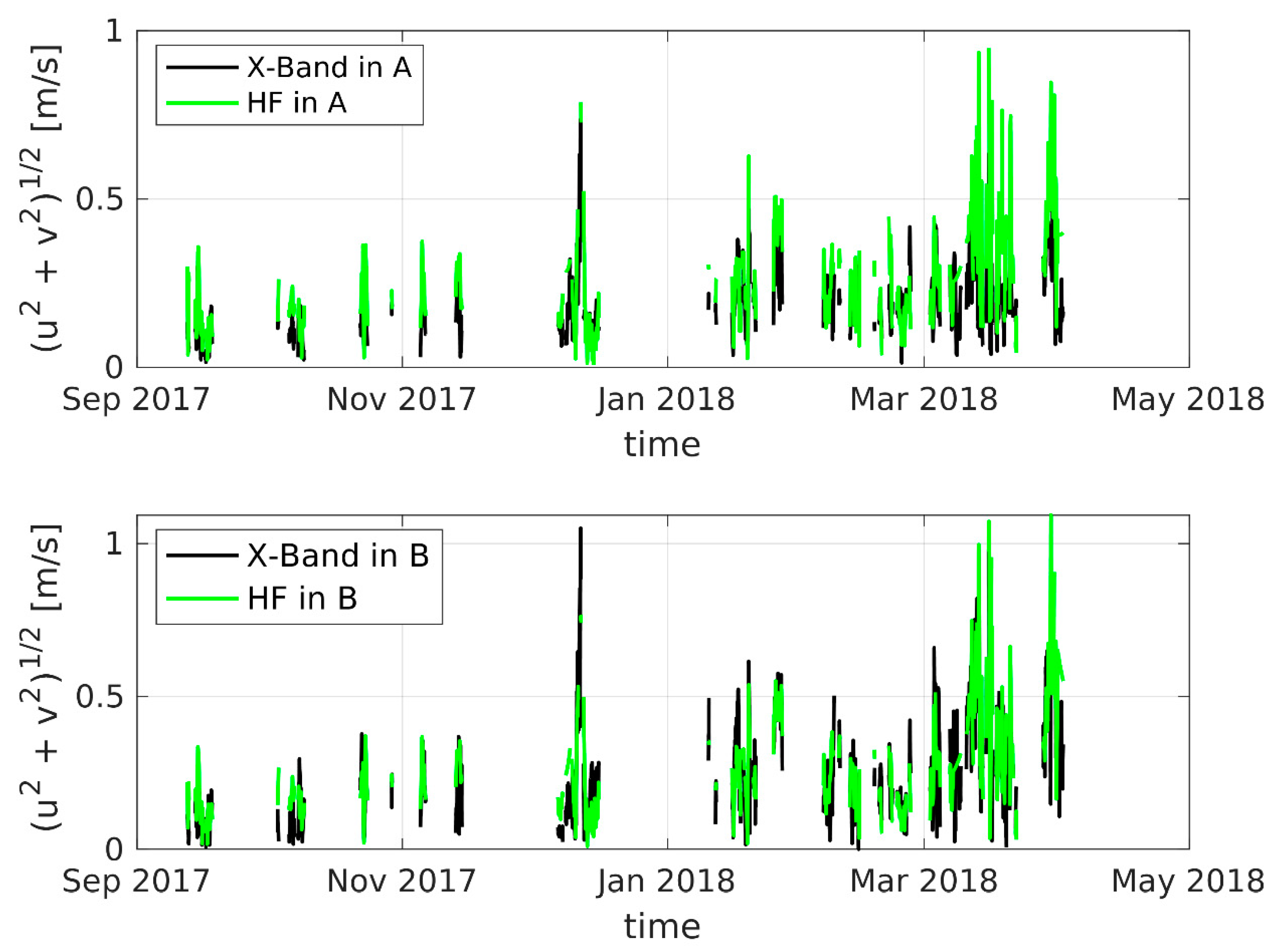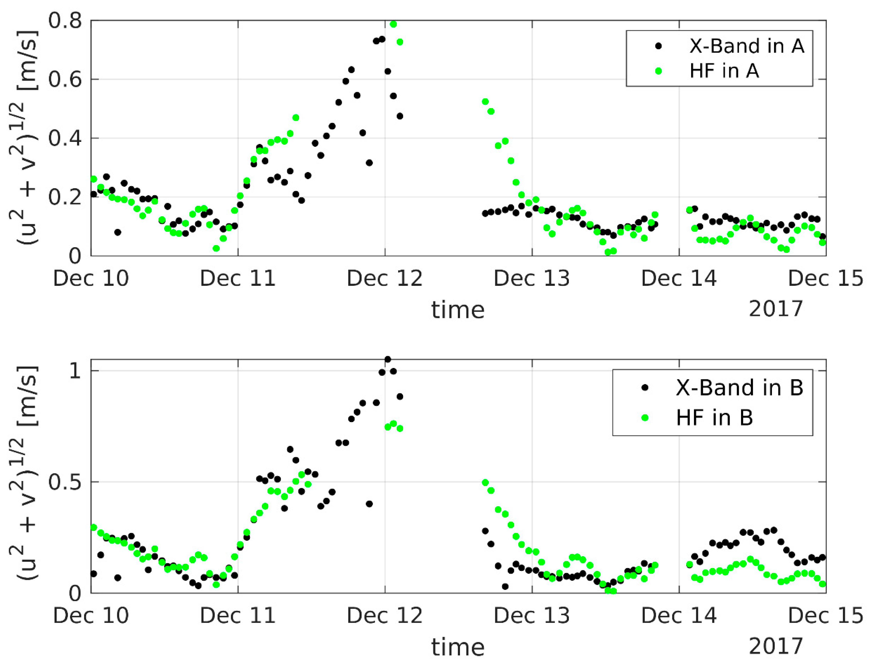Figure 6 shows the resulting time signature of the velocity intensity at overlapping points A and B as derived by the two instruments; a close up of a shorter timeslot is shown in Figure 7 only for clearer visualization purposes. 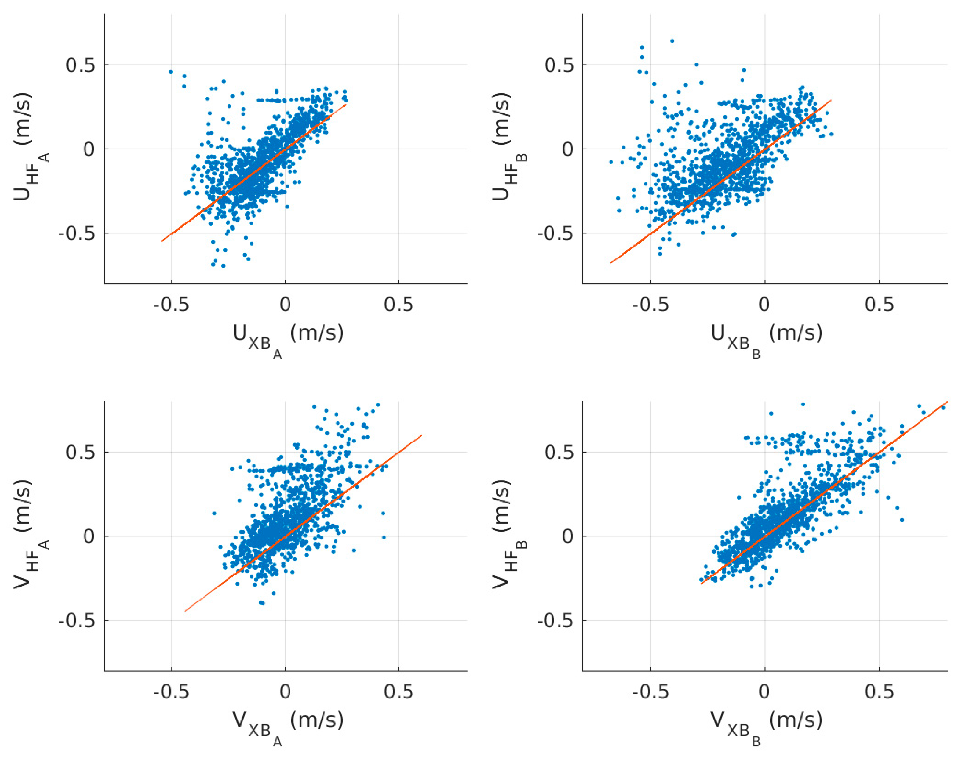Figure 8 finally reports a scatter plot of the HF and X-band surface velocity components in A and B, separately.

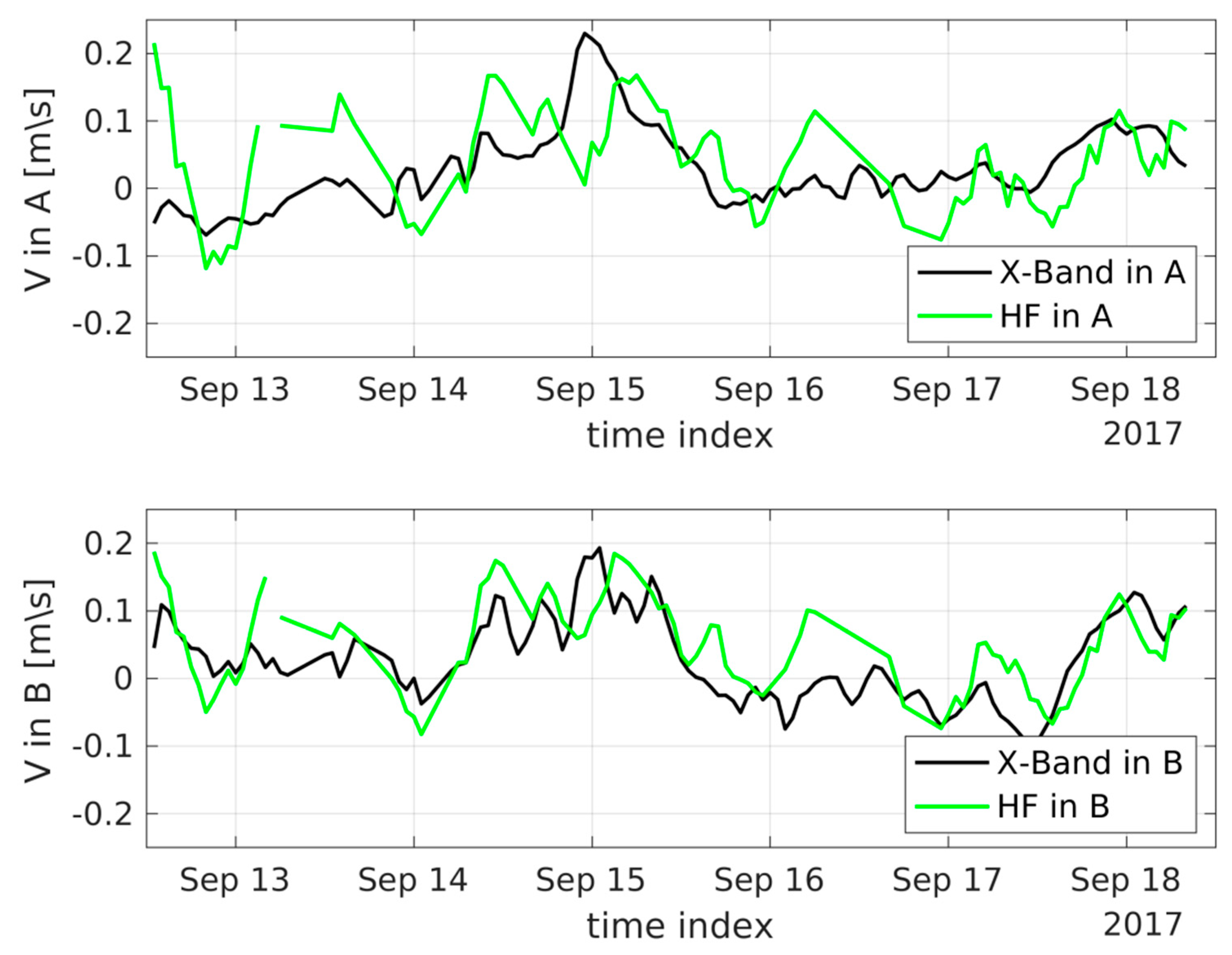
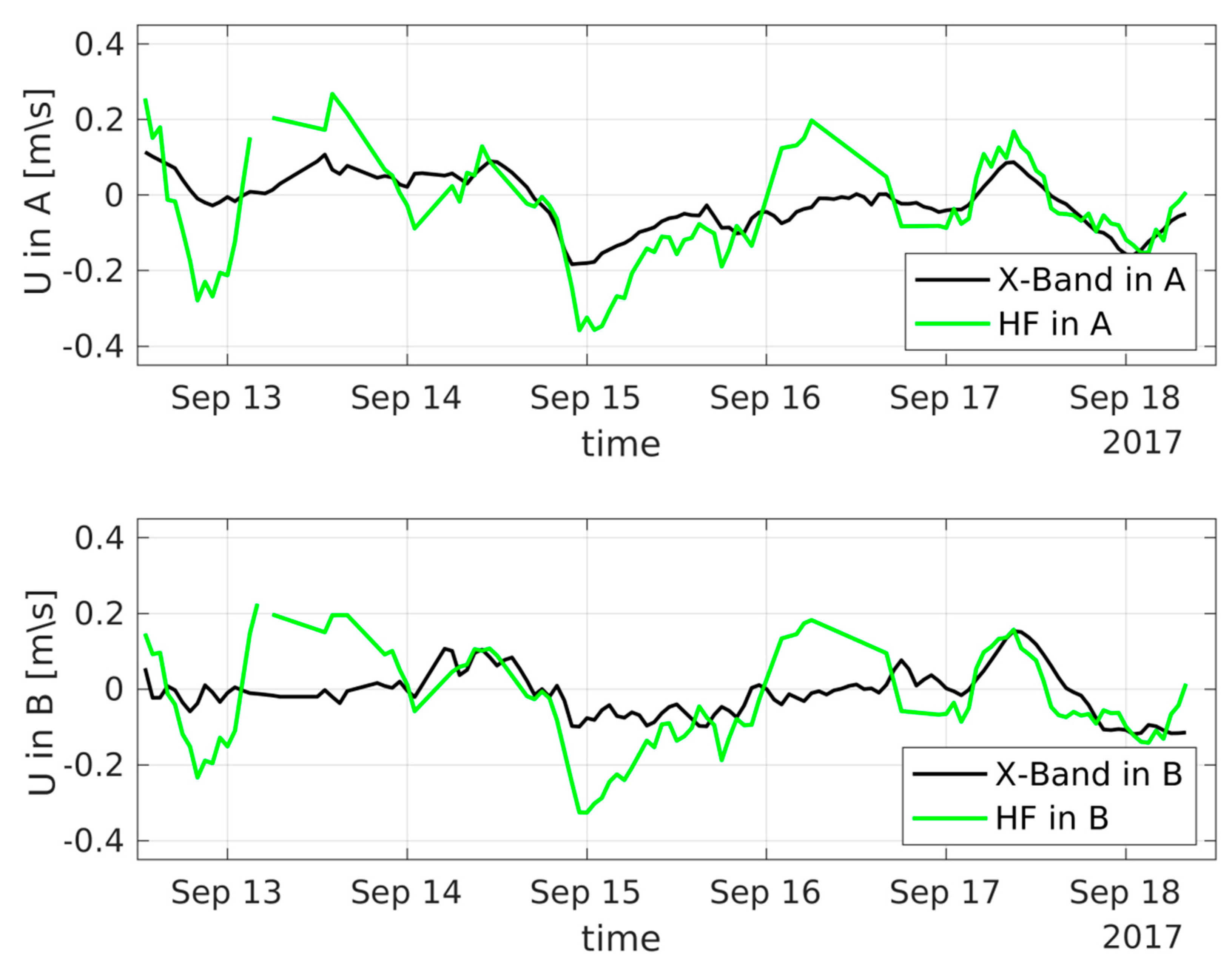
As a final step, we show in Figure 9 and Figure 10 a close up on the measured components over a reduced time range (12 September 2017 to 18 September 2017) characterized by the time-average condition reported in Figure 3 for that time range. The reported time-series are shown at regular hourly time spacing. The corresponding root mean square errors, for the shorter set, were 0.1 m/s and 0.12 m/s for U in A and B, respectively, and 0.07 m/s and 0.05 m/s for V in A and B, respectively. It is interesting to note the substantial disagreement in northward components at location A, occurring at 15 September and neighboring times (upper panel of Figure 9). Here, the X-band measurements showed a positive peak as opposed to the local decrease captured by the HF measurements. The computed spatial standard deviation of the northward component, at this time (and neighboring times), exceeded the 90% of its maximum values, revealing the existence of a high spatial variability that might be not completely captured by the low resolution grid of the HF radar.

Similarly, the eastward components at the same time locations were also characterized by a local overestimation of the velocity intensity by the HF radar compared to the X-band one, at location A (upper panel of Figure 10). Additionally, in this case, a field spatial standard deviation above 85% of the maximum level was found. At early times (i.e., between 12–13 September (Figure 9 and upper panel of Figure 10), discrepancies between HF and X-band data were associated with values of the spatial standard deviations ranging between 50% and 70% of the maximum value for the northward component, and around 50% of the maximum value for the eastward component, revealing a quite significant spatial variability that may affect the HF derived values in the analyzed sea condition.

4. Conclusions

In this work, the surface current fields measured by an X-band radar were compared with those provided by a HF-band radar. The comparison showed good agreement between the measures, although some discrepancies were also detected. At this stage, we cannot rigorously explain the nature of such differences among the data. A possible explanation resides in the different spatial scales that can be captured by the two tools. The HF radar is likely to over-smooth the small-scale features typically occurring in coastal waters or complex nearshore bathymetries. The high spatial variability of such features might not be completely captured by the HF coarse resolution, largely remaining a not-resolved sub grid process. On the other hand, the higher spatial resolution of the X-band radar allows for the capture of finer processes that are likely to carry higher sources of field local variance. The second possible source of differences between the HF and X-band derived currents is the inherent limitation of the latter, which loses accuracy when estimating surface currents in under-developed sea conditions. An important aspect that emerges from this work is the possible integrated usage of the two instruments, which exploits the advantages provided by the individual parts (wider spatial coverage for the HF band and higher spatial resolution for the X-band). Consequently, more accurate measurements of surface currents can be carried out by the combined system on large spatial domains still capturing smaller scale effects in the nearshore area. The analysis carried out in this study represents a preliminary assessment for the system performance. Its effective usage aimed at unveiling the physical processes of oceanographic relevance still remains beyond the target of this work. A physically-oriented application aiming at enlarging the background of physical oceanography is clearly needed to fully exploit the system potential, and will be explored in a future study.