Monitoring Urban Green Infrastructure Changes and Impact on Habitat Connectivity Using High-Resolution Satellite Data


1
Division of Geoinformatics, Department of Urban Planning and Environment, KTH Royal Institute of Technology, Teknikringen 10A, 10044 Stockholm, Sweden
2
Division of Sustainability Assessment and Management, Department of Sustainable Development, Environmental Sciences and Engineering, KTH Royal Institute of Technology, Teknikringen 10B, 10044 Stockholm, Sweden
*
Author to whom correspondence should be addressed.
Remote Sens. 2020, 12(18), 3072; https://doi.org/10.3390/rs12183072
Submission received: 21 July 2020
/
Revised: 4 September 2020
/
Accepted: 15 September 2020
/
Published: 19 September 2020
(This article belongs to the Special Issue Smart City Development and Remote Sensing Application in Urban Ecology)
Abstract
:In recent decades, the City of Stockholm, Sweden, has grown substantially and is now the largest city in Scandinavia. Recent urban growth is placing pressure on green areas within and around the city. In order to protect biodiversity and ecosystem services, green infrastructure is part of Stockholm municipal planning. This research quantifies land-cover change in the City of Stockholm between 2003 and 2018 and examines what impact urban growth has had on its green infrastructure. Two 2018 WorldView-2 images and three 2003 QuickBird-2 images were used to produce classifications of 11 land-cover types using object-based image analysis and a support vector machine algorithm with spectral, geometric and texture features. The classification accuracies reached over 90% and the results were used in calculations and comparisons to determine the impact of urban growth in Stockholm between 2003 and 2018, including the generation of land-cover change statistics in relation to administrative boundaries and green infrastructure. For components of the green infrastructure, i.e., habitat networks for selected sensitive species, habitat network analysis for the European crested tit (Lophophanes cristatus) and common toad (Bufo bufo) was performed. Between 2003 and 2018, urban areas increased by approximately 4% while green areas decreased by 2% in comparison with their 2003 areal amounts. The most significant urban growth occurred through expansion of the transport network, paved surfaces and construction areas which increased by 12%, mainly at the expense of grassland and coniferous forest. Examination of urban growth within the green infrastructure indicated that most land area was lost in dispersal zones (28 ha) while the highest percent change was within habitat for species of conservation concern (14%). The habitat network analysis revealed that overall connectivity decreased slightly through patch fragmentation and areal loss mainly caused by road expansion on the outskirts of the city. The habitat network analysis also revealed which habitat areas are well-connected and which are most vulnerable. These results can assist policymakers and planners in their efforts to ensure sustainable urban development including sustaining biodiversity in the City of Stockholm.
1. Introduction
Over the past two decades, the City of Stockholm, Sweden, has grown substantially and is now the largest city in Scandinavia. Its population has risen by over 28% since the year 2000. Urbanization due to population increase is placing pressure on the green areas in and around Stockholm, which are valuable for the maintenance of biodiversity and ecosystem services. However, green areas are often reduced and fragmented as urban areas grow, leading to potential negative environmental impacts, not least in regard to biodiversity [1]. A concept for promoting biodiversity and ecosystem services in planning is green infrastructure, which can be defined as a network of natural and seminatural areas, designed and managed to deliver a wide range of ecosystem services [2]. Green infrastructure is promoted by the European Commission as a key instrument for the conservation of ecosystems in the EU biodiversity strategy to 2030 [3]. In Sweden, action plans for green infrastructure have been developed in all counties [4], including Stockholm County [5].
Urban green infrastructure has gained much interest as a planning tool for sustainable urban development, e.g., [6,7], and needs to address the scale, governance level and goals of the city, e.g., [8]. The City of Stockholm forms the center of this urban region, and locally adapted green infrastructure plays an important role in its planning process [9]. Stockholm City has a number of environmental goals including that its green infrastructure should be well-managed in order to promote biodiversity and ecosystem services [10]. At the same time, the city intends to build 140,000 new housing units by the year 2030 [11] in order to meet the demand for housing from an increasing population. Timely and accurate mapping of urban land-cover changes and assessment of environmental impact is therefore important to facilitate decision-making in urban planning for sustainable urban growth.
Given its synoptic and spatially consistent geometric detail delivered at high-temporal frequency [12,13], remote sensing data provides valuable geographic information for mapping and monitoring of urban land-cover change. Numerous studies have utilized medium-resolution satellite data to perform urban land-cover mapping and urban growth monitoring, e.g., [14,15,16,17]. Satellite data-based classification of urban environments is challenging because of the increased complexity, particularly at higher spatial resolutions, of land-cover features found within them [18,19,20]. Momeni et al. [21] found that spatial resolution has the most influence on classification accuracy in complex urban environments and that high-resolution sensors provide a clear advantage in this context. High-resolution data, such as IKONOS, QuickBird or WorldView data, has proven useful in the classification of urban land-cover types, e.g., [19,22,23,24] but has also been used to map various kinds of fauna habitat, e.g., [25,26], green and blue structures, e.g., [27,28,29] and ecosystem services, e.g., [23,30].
Turner et al. [31] and Pettorelli et al. [32] have pointed out that remote sensing data is underused in and holds great potential for studies monitoring biodiversity. The use of remote sensing at a medium resolution to monitor biodiversity has seen extensive development [33]. Mairota et al. [34] highlight the high-resolution data that remote sensing can deliver on habitat quantity and quality but note hindrances that have limited its use for this purpose. Boyle et al. [35] demonstrate the utility of high-resolution optical remotely sensed data for monitoring land-cover change for conservation but also found that its use was very limited (approximately 10% of the land-cover studies used satellite imagery of 5 m or less in the research published by three major conservation biology journals). The limited usage appeared to be linked to the acquisition cost of high-resolution imagery, especially given the freely available lower resolution alternatives, and the authors called for greater accessibility to high-resolution imagery in this regard. There are to date relatively few high-resolution remote sensing-based land-cover assessments of impacts on habitat and related biodiversity components from urbanization. This has usually been undertaken based on maps or information derived from aerial photos or surveying and with the aid of information from aerial scanners [36] and, e.g., [37,38]. With the increasing availability of high-resolution satellite data providing detailed, accurate and repeated earth observations, there is a need to investigate its full potential for green infrastructure monitoring.
The use of object-based image analysis (OBIA) for land-cover classification based on high-resolution data has been shown to outperform pixel-based approaches [39,40], particularly in combination with the support vector machine (SVM) algorithm [41,42]. The research of Momeni et al. [21] confirms that the classification of high-resolution satellite data over complex urban environments through the use of OBIA and the SVM classifier is an optimal combination to ensure high land-cover classification accuracy. This approach was employed in this study. The resulting urban land-cover maps based on WV-2 and QB-2 data captured on different dates over the City of Stockholm were used to make spatiotemporal comparisons and evaluate environmental impacts, such as on the green infrastructure. High-resolution satellite imagery is necessary as the main data source given the size of the study area and the analyses to be performed.
While habitat amount has been identified as the largest contributing factor to species persistence and abundance [43,44], habitat connectivity also plays a significant role in biodiversity conservation due to its effect on metapopulation dynamics [45]. Network analysis of habitat connectivity offers a possibility to examine the configuration and interconnections of habitat patches and their relative importance for the maintenance of biodiversity components. Graph-theoretic approaches to modeling habitat connectivity, which represent the habitat as a set of nodes (habitat patches) and links (connecting elements), have been developed [46,47,48] and are increasingly used in conservation planning and ecological assessments [49,50,51]. Of the many graph-theoretic indices available, the probability of connectivity index (PC) has characteristics that make it well-suited to the assessment of functional connectivity across a range of scales. PC is based on a probabilistic connection model and its value is defined as the probability that two randomly selected habitat patches are connected based on the defined dispersal behavior and the structure of the landscape in question. Saura and Pascual-Hortal [52] developed the index and compared it to other landscape indices and their respective detection capabilities, where it performed well. Saura and Rubio [53] further conceptually developed this index and demonstrated its flexibility in analysis by showing how it can be separated into three component fractions representing different ways in which a node can contribute to habitat availability in the network. A particular advantage of one of the fractions is that it estimates a patch’s significance as a connecting element, assessed independently of its area-related importance. The equivalent connected area (ECA) index, which can be derived directly from PC, is also useful for comparing temporal changes to landscape connectivity since it represents the size of one habitat patch that would provide the same connectivity probability value as the habitat pattern in the landscape examined [54]. The PC index has been increasingly used in landscape ecological assessments [55,56,57]. PC, its component fractions and ECA have been used in this study to assess changes in habitat availability and connectivity for two species sensitive to urbanization in Stockholm City.
While numerous studies have used landscape connectivity indices, assessment and modeling to evaluate urban green infrastructure for planning purposes [58] and, e.g., [59,60,61], few studies have employed connectivity indices for the purpose of monitoring spatiotemporal change in urban green infrastructure. To the best of our knowledge, there has not yet been a study that utilizes the PC and ECA indices in combination with high-resolution satellite classifications to assess spatiotemporal changes in specific species habitat connectivity and availability in an urbanizing area. The objective of this research has been to investigate urban growth between 2003 and 2018 in Stockholm City in relation to administrative boundaries and to the green infrastructure, including its impact on the connectivity of the habitat network for selected sensitive species by calculating PC and ECA. The results provide answers not only to questions related to spatially explicit quantities of urban growth and green infrastructure loss, but also as to how biodiversity components have likely been affected by recent and nearby urbanization through network analysis. Information like this can facilitate planning and decision-making in Stockholm in relation to future urban development and environmental conservation at different scales.
2. Materials and Methods
2.1. Study Area and Data Description
The City of Stockholm covers approximately 188 km2 of land area [62]. It is surrounded by and contains parts of the green infrastructure that is defined on a regional level, as mentioned in the Introduction [5,63], often formed as “green wedges”, i.e., large swaths of natural and seminatural vegetation that lead from the surrounding rural areas in towards the more densely built-up urban city center. The wedges often contain nature reserves or national parks, such as Stockholm’s National City Park, and are part of Stockholm regional planning to ensure recreational opportunities, habitat for wildlife and the provision of ecosystem services [63]. Yet, the City’s natural areas are under pressure from the region’s growing population and the increasing demand for built-up areas. Plans for the creation of 22,000 new dwellings each year up to 2030 are already underway [63]. This study investigates the impact of urban expansion on green areas and green infrastructure in Stockholm City between 2003 and 2018.
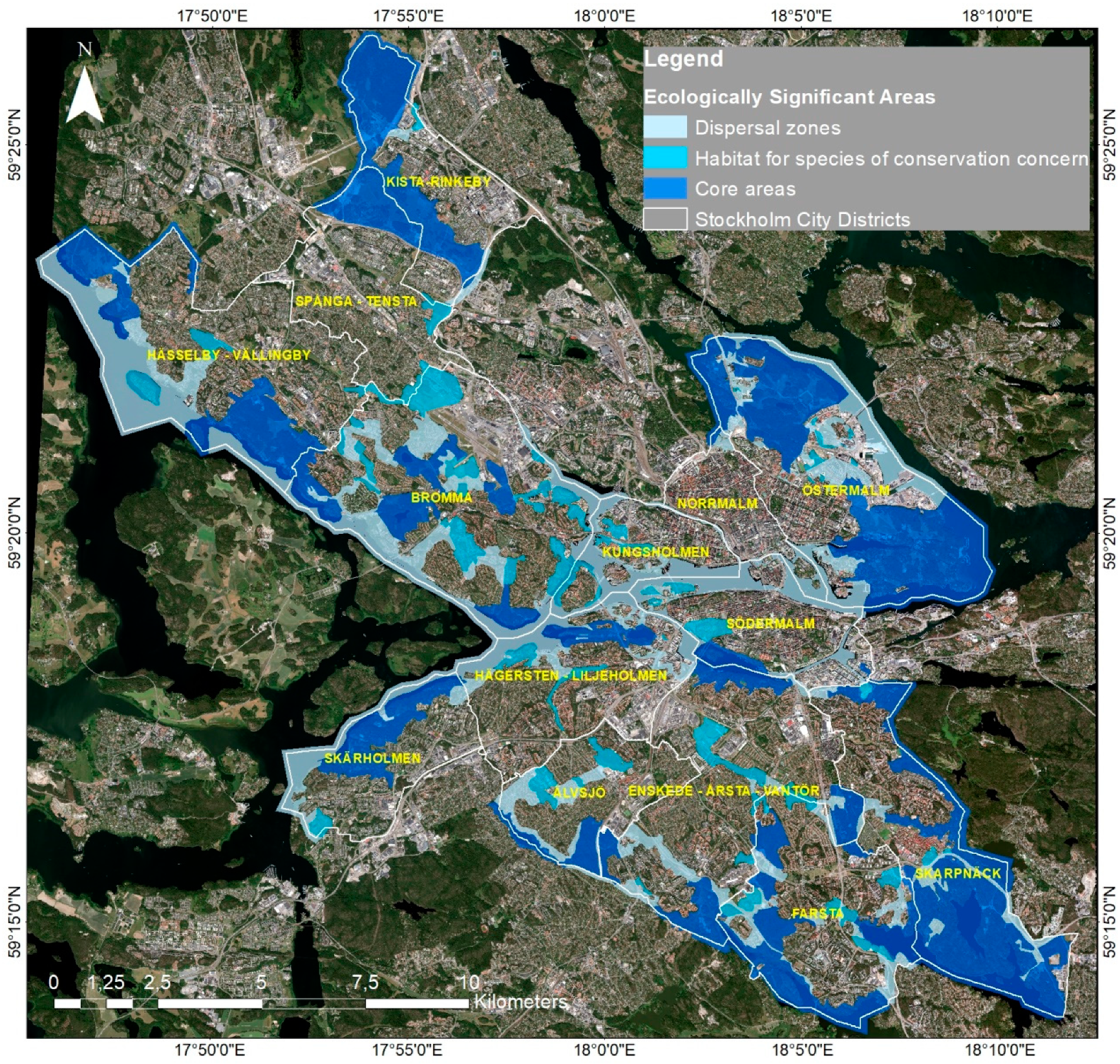
Stockholm City is the study area and comprises 14 city districts (Figure 1). The total analysis area is approximately 216 km2 including water. Land-cover classes in the city that could be identified from the satellite imagery with the selected classification techniques are buildings, transport/construction sites, urban green space, grass/open fields, coniferous forest, deciduous forest, rock outcrop, barren land/soil, agricultural land, wetlands and water. The transport/construction class includes roads, railway, airport runway and pavement in general, as well as construction and industrial extraction sites. Prime examples of urban green space are city parks, allotment areas or gardens, but the class also includes any otherwise undesignated green area composed of a mix of trees, shrubs and grass in or around urban areas.
Two WorldView-2 (WV-2) images at product level Standard 2A captured on 4 July 2018 and covering slightly more than the geographic area of Stockholm City were acquired for classification. Two scenes of QuickBird-2 (QB-2) images at product level Standard 2A captured on 14 June 2003 (covering approx. 90% of Stockholm City) and 6 September 2005 (covering approx. 10% of Stockholm City) were also acquired. Efforts were made to obtain images from the peak of the vegetation season to take advantage of spectral differences between green and gray areas and in order to avoid the detection of nonpermanent changes caused by seasonal differences. The same four multispectral bands from both sets of imagery were used for segmentation and classification, namely the blue, green, red and near-infrared bands. Only four of the eight multispectral bands available in the WV-2 data were used in order to reduce processing time and to not exceed computer memory constraints as well as to match the spectral input for the segmentation and classification of the 2003 QB-2 imagery.
The City of Stockholm has invested in the development of geographic information about its green infrastructure in order to facilitate the integration of biodiversity aspects into planning and environmental assessment. Stockholm City developed a geographic dataset representing its green infrastructure [64]. This polygon vector dataset was created in 2013 based on the city’s geographic ecological information sources with reference years varying between 1995 and 2010, such as the oak database, the city biotope map and its species observation data archive (ArtArken [65]), as well as on representative habitat networks. These habitat networks represent selected sensitive species and were developed by Mörtberg et al. [66,67], based on available geographic data and expert knowledge. Likely impacts on the habitat networks were estimated based on a then-current city planning scenario, but they have not yet been used in comparison with spatiotemporal assessment of landscape changes from urban growth.
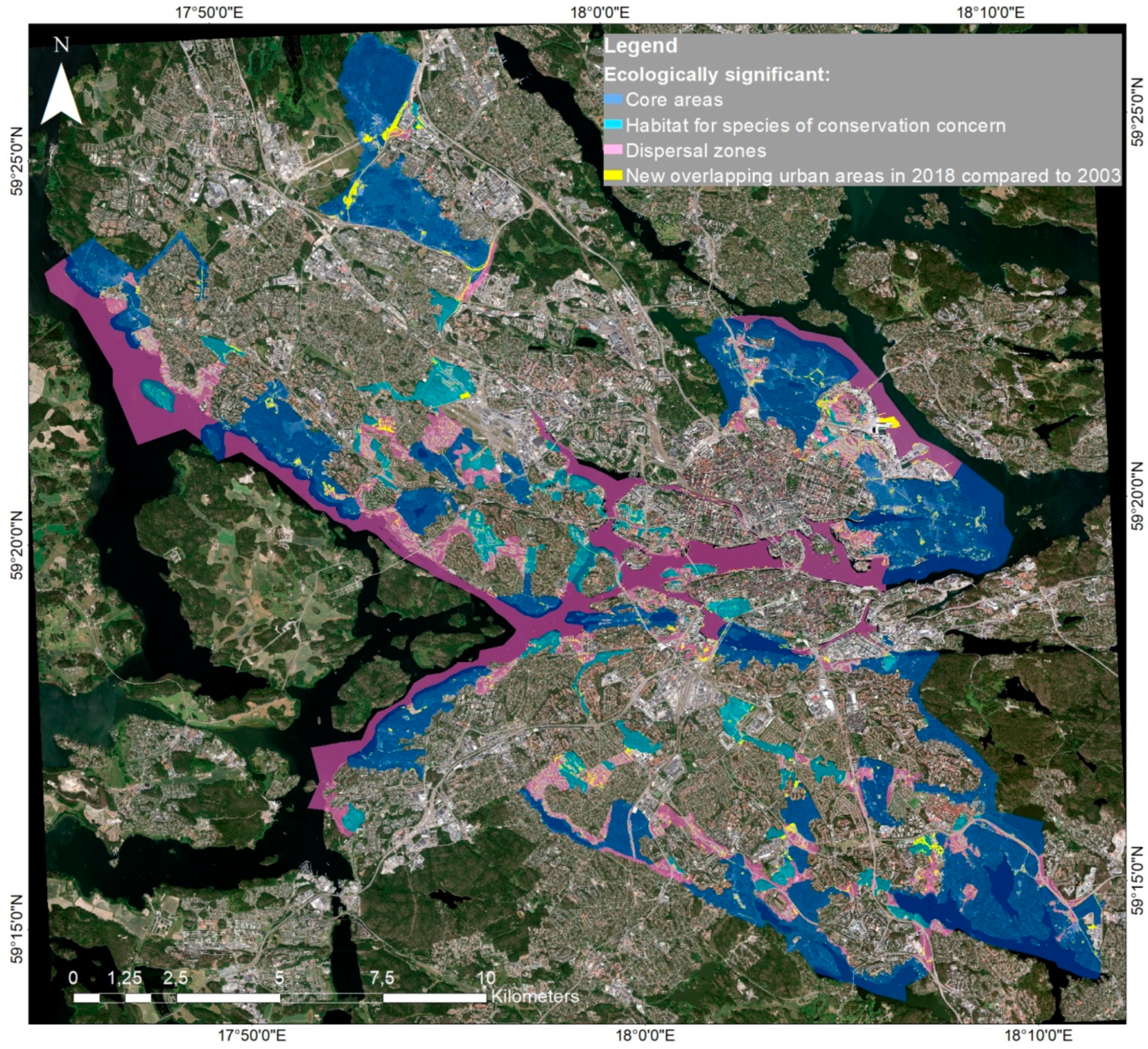
Ecologically significant areas in the green infrastructure dataset are divided into three categories, referred to as ecologically significant (1) core areas, (2) habitat for species of conservation concern and (3) dispersal zones. The ecological qualities of the core areas mean that they often host a wide variety of plant and animal species and play an important role in maintaining ecosystem functions. Habitat for species of conservation concern is based on occurrences of red-listed species and their habitat requirements. Dispersal zones are areas important for the movement of species between habitat patches or core areas.
2.2. Methodology
2.2.1. Image Preprocessing
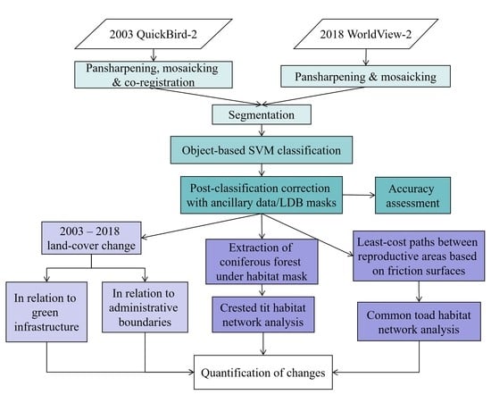
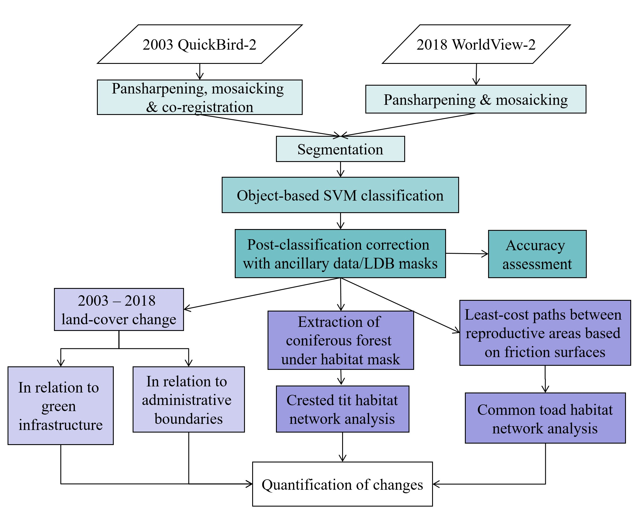
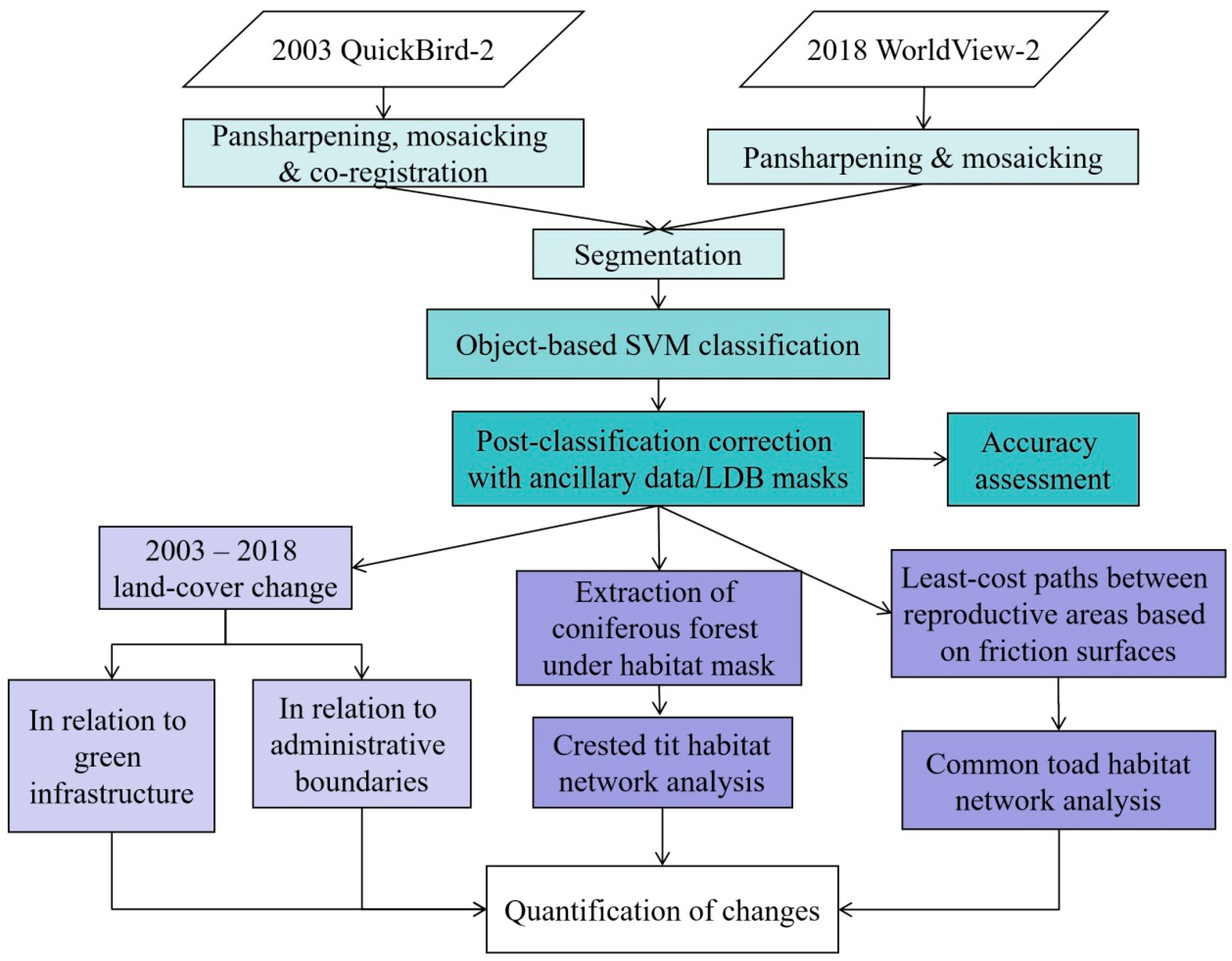
An overview of the study methodology is presented in Figure 2. Processing Standard 2A provides WV-2 and QB-2 images that are radiometrically corrected and orthorectified. Thus, only two preprocessing steps were necessary. First, the WV-2 and QB-2 multispectral bands (spatial resolutions: 2 and 2.4 m, respectively) were pansharpened to 0.5 and 0.6 m, respectively, based on their panchromatic bands. The higher spatial details of the pansharpened images were deemed essential for improved classification of small houses and small urban green spaces such as allotment areas and gardens [68]. The pansharpening was performed using the automatic image fusion algorithm in PCI Geomatica developed by Zhang [69]. Secondly, since two scenes of both types of imagery were required to cover the geographic area of Stockholm City, both pairs of images were mosaicked, also using PCI Geomatica. Once these steps were completed, however, a slight shift (around 5–10 m) due to a residual geolocation error was discovered between the QB-2 and WV-2 images. Given the higher geolocation accuracy of the WV-2 sensor (CE90 < 3.5 m) compared to QB-2’s (CE90 23 m) [70,71], we used the WV-2 image as reference and coregistered the images using the automatic coregistration image workflow available in ENVI version 5.3 (Exelis Visual Information Solutions, Boulder, Colorado). The final images were correctly coregistered with subpixel residual error.
2.2.2. Segmentation and Classification of Satellite Data
Object-based image analysis (OBIA) has become widely used in recent years as a key step in the classification of high-resolution data thanks to its frequently superior performance than many pixel-based approaches [19,72,73]. OBIA was deemed appropriate for this study given the resolution of the data and the focus of the classifications, which is on nonurban vs. urban land-cover types. eCognition Developer software [74] was used to segment, extract features from and classify the two sets of images. Scale parameters of 100 for 2003 and 125 for 2018 were used for segmentation. The homogeneity criteria of shape and compactness were set at 0.1 and 0.5, respectively, for both years. Parameter selection was based on trials and yielded the most appropriate objects for classification by virtue of their close representation of discrete areas of various land/cover types and structures in the images.
Training samples were gathered for 17 classes initially: 6 classes for buildings based on varying reflectance properties of building materials (for example, copper roofing generally had greater reflectance values than concrete roofing), 2 for transport lines and construction sites, 1 for urban green space, 2 for open grassland and grass sports fields, 1 for coniferous forest, 1 for deciduous forest, 1 for bare rock, 1 for barren land/bare soil, 1 for water and 1 for shadow. Following classification, spatial relationships between classes such as relative border thresholding were used to correct object misclassifications. In this way, many isolated misclassifications were corrected within the coniferous forest, deciduous forest and water classes in particular. Objects identified as shadow were assigned to the class with which they shared the largest relative border. Roads misclassified as buildings were corrected using a length threshold.
Classification of a wetland category was tested but it was heavily confused with both the coniferous forest and rock outcrop classes. Wetlands cover less than 1% of Stockholm City. Given their limited coverage and significant confusion with other classes, wetland areas were masked in based on the corresponding class in a 10 m national land-cover dataset [75] and checked manually post-classification. Agricultural fields were also incorporated as a separate class in this way, using a mask based on the appropriate category of the national land-cover dataset.
Various object features and classification algorithms were tested and compared. A successful approach used in previous research [76] with slightly lower resolution imagery was adopted here and yielded good results. This involved a support vector machine (SVM) classification algorithm trained with statistics from one textural, two spectral and three shape data features. Spectral band mean and standard deviation were used as well as Roundness, Asymmetry and Rectangular fit shape features and the Gray-Level Difference Vector (GLDV) Entropy (all directions) texture feature contributed to improved classification results.
To further improve the classification results and their comparability, corrective rules were used under urban and forest masks to reclassify noted problematic areas. A low-density built-up area mask from a previous 2005 classification was manually verified/edited and used to standardize the classifications for building and transport areas that had not changed. Unchanged major transport lines from 2003 were compared to those in the 2018 classification and added where necessary. A forest mask based on the relevant classes from the national land-cover dataset [75] was applied to improve deciduous forest classification where shadow was confused with coniferous forest in the 2018 classification. Green roofing added during the study period was controlled for through an overlay check of conversion from urban to green structure classes and misclassifications were manually corrected. Once post-classification corrections were completed, a minimum of 500 validation sample vector points for each land-cover class were used for accuracy assessment. The points were manually recorded for both years with the satellite imagery, historical Google Earth images and local knowledge of the study area as comparing sources.
2.2.3. Landscape Change Analysis
Land-Cover Change According to Administrative Boundaries and Within the Green Infrastructure
Based on the 2003 and 2018 classifications, the land area percent change in urban areas (comprised of the buildings and transport/construction classes) and in green areas (comprised of deciduous/coniferous forest, urban green space, grasslands, agricultural land, barren land, wetlands and bare rock) per city district was calculated. This information reveals where and relatively how much change occurred in different areas within the city. Urban land-cover change in relation to the three types of ecologically significant areas of the green infrastructure as identified by the city was also investigated. The increase in the amount and percentage of urban overlap in these areas was quantified and the change shown graphically.
Change in Habitat Network Connectivity
Habitat connectivity plays a significant role in biodiversity conservation due to its effect on metapopulation dynamics [45], even if habitat amount has been identified as the major contributing factor to species persistence and abundance [43,44]. Habitat networks for selected species sensitive to urbanization were developed by Mörtberg et al. [66,67], including the European crested tit (Lophophanes cristatus) and the common toad (Bufo bufo).
The crested tit is strongly tied to mature and old pine and spruce forests where it requires access to deadwood in standing trees for nesting. It is also sensitive to fragmentation since it avoids open areas and prefers relatively large (10–25 ha), well-connected coniferous forest patches [77,78,79,80]. Information on habitat requirements, gathered by a literature review and interviews with experts by Mörtberg et al. [67], provided the basis for assumptions, criteria and parameters used for the crested tit habitat network analysis in the current study (Appendix A).
Patches for the crested tit habitat analysis were derived by extracting all mature and old coniferous forest from the classifications under a mask of the crested tit habitat geographic dataset created by Mörtberg et al. [67]. All patches with an area of 2 ha or greater were selected initially for analysis since this is below the assumed 3 ha minimum requirement for nesting areas but is still assumed large enough to be used for foraging [67]. A threshold for patch area was necessary for two reasons: to limit the number of patches in order to reduce the required computational resources so that the habitat network analysis could be performed, and because, upon comparison, it was found that larger patches tended to be characterized by higher habitat quality (based on age and type of coniferous forest), one of the main attributes of the crested tit habitat.
Patches that crossed the city boundary were kept in their entirety so as not to unduly influence the network analysis through truncated patches. The preliminary habitat patch selections for 2003 and 2018 were then cross-checked and modified if necessary to ensure that approximately the same patches were included for both years and that none were eliminated because of minor misclassifications or slightly different delineations. Patches with areas down to 1 ha were added where necessary. The resulting habitat networks for both years contain approximately 230 patches each with an average patch size of about 9 ha.
Six of the 13 amphibian species present in Sweden can be found in Stockholm County and Mörtberg et al. [66] selected the common toad as a study object for the development of a habitat network tool. Like other amphibians there, it is dependent on both land and water during its lifecycle and reproduces in water. While the toad is not as threatened by fish since its eggs are poisonous, can travel relatively long distances and is somewhat of a generalist, it is nonetheless sensitive to small barriers and traffic. As highlighted by Mörtberg et al. [66], this makes it suitable as a representative species in landscape ecological assessments of urbanization where habitat fragmentation is addressed and where there is less focus on local habitat variations. While toad populations in Stockholm City have become stable thanks to recent local initiatives, they are nonetheless still under pressure from urban expansion [81,82]. Again, information on dispersal and habitat requirements, as gathered by a literature review and interviews with experts by Mörtberg et al. [66], provided the basis for assumptions, criteria and parameters used for the common toad habitat network analysis in the current study (Appendix A).
Mörtberg et al. [66] created a geographic data layer of common toad reproductive areas in Stockholm City based on proximity to water and appropriate land-cover types. This dataset was compared to urban areas (transport network and buildings) in the 2003 and 2018 classifications and those reproductive locations that overlapped more than 50% were removed. Patches within the City of Stockholm and up to 300 m from its boundaries with an area of 500 m2 or greater were selected. These areal and spatial limitations were necessary in order to reduce the required computational resources so that the habitat network analysis could be performed. This yielded a 2003 reproductive area dataset of 838 patches with an average patch size of 0.04 ha and a 2018 dataset of 811 patches also with an average patch size of 0.04 ha.
The next step was to construct a friction surface representing in numeric form the resistance or degree of difficulty that a toad might experience while moving through the Stockholm City landscape. Two surfaces (for 2003 and 2018) were created based on the land-cover classifications where each land-cover category was associated with a numeric cost. The cost was established based on the dispersal profile for the common toad outlined in Mörtberg et al. [66] who had also created an example friction surface in 2006. The costs for each land-cover type present in the high-resolution classifications as well as from the study by Mörtberg et al. [66] are listed in Table 1.
Based on the friction surfaces, least-cost path networks connecting the reproductive areas were created for both 2003 and 2018. Mörtberg et al. [66] noted that dispersal or movement distances for the common toad often do not exceed 2 km across optimal (low-cost) land-cover. For this reason, cost paths longer than 2 km were removed from the networks.
Conefor 2.6 is a freely available software package that can calculate a range of network connectivity indices [83] and is here used to calculate the probability of connectivity (PC) metric, using the following function:
where and correspond to habitat attributes of patches i and j, of which the area is used in this study. is the maximum landscape attribute and therefore the same as the total landscape area in this case. is the maximum product probability of dispersal and equals the product of probabilities of traveling through adjacent habitat patches to get to a destination patch. It is used in index calculation if larger than the probability of direct dispersal ().
The contribution of landscape elements (patches and links) to overall habitat connectivity and availability can be calculated from the percentage of variation in PC () caused by the removal of each single element from the landscape [46,52]:
where is the difference in the value of PC when element k is present compared to when it has been removed from the network. Following removal, any maximum product probability paths that previously went via k have to be rerouted through other elements available in the network. Saura and Rubio [53] demonstrated how can be partitioned into three fractions which represent various ways in which a patch or node can contribute to habitat availability and connectivity in a network:
is a measure of internal connectivity and corresponds to x (Equation (1)) when i = j = k and . It measures the habitat availability in the patches themselves independent of other elements in the network. is similar to other measures of flux [46,84,85] but considers maximum product probability paths () instead of probabilities of direct dispersal (). It corresponds to the case where i = k or j = k, but i ≠ j. depends solely on the topological position of a connecting element in the landscape network and is a measure of a patch or link k’s contribution to connectivity between other habitat patches. It is the partial sum of (Equation (1)) where i ≠ k, j ≠ k and k is part of the maximum probability path that lies between them. For a more detailed explanation of the PC metric and its component fractions, see Saura and Rubio [53].
For the crested tit habitat network analysis, patch nodes and the distances between them (measured from patch perimeter) were generated using the ArcGIS extension Conefor Inputs [86] and are used as input files for the calculation of PC and its component fractions. Dispersal or movement distances and their probabilities were selected based on species profile information reported by Mörtberg et al. [67]. Small birds can move easily through a landscape thanks to their ability to fly but given the assumed reluctance of the crested tit to cross open spaces, a median dispersal distance of 200 m was chosen corresponding to probability 0.5. An assumed maximum connection distance of 2000 m was used. Connectivity indices were calculated based on the nodes and distances derived from the coniferous forest habitat datasets extracted from the 2003 and 2018 classifications.
For the common toad habitat network analysis, patch nodes and probabilities of connections between them were used as input files for the calculation of PC and its component fractions. The least-cost path networks provided cost information for each path and in order to convert these to probabilities of usage, the lowest cost available in the network (8.485 in both 2003 and 2018) was divided by the cost of the path in question. This yielded internode path probabilities between 0 and 1. Changes in PC as well as in its component fractions were compared between years for both habitat networks.
An index useful for comparing temporal changes to landscape connectivity can be derived directly from PC. This is the equivalent connected area (ECA) which is defined as the size of one habitat patch that would provide the same connectivity probability value as the habitat pattern in the landscape under examination [54]. It is calculated by taking the square root of the numerator in the PC index (Equation (1)) and has area units. Relative change in ECA (dECA) can also be evaluated and was calculated for this study in the following way:
dECA is also of interest since it can be directly compared to dA, which is the change in the total amount of habitat area calculated in the same way. ECA, dA and dECA for the landscapes in the years evaluated are therefore calculated.
3. Results
3.1. Classification of High-Resolution Satellite Data
Table 2 shows the accuracy scores for the segmentation-based SVM classifications after post-classification corrections. A 93% overall accuracy (kappa: 0.92) was achieved for 2003 and over 91% overall accuracy (kappa: 0.90) for 2018. The producer’s and user’s accuracies show more specifically how well each land-cover type was classified. The accuracies for all classes were above 80% and thus satisfactory. There was some confusion between the building and transport/construction classes and between barren land and transport/construction, which can be expected given how spectrally similar these classes usually are. The coniferous forest class in the 2018 classifications is slightly overestimated at the expense of deciduous forest and urban green space, due in part to longer shadows in the 2018 imagery which were at times classified as coniferous forest within those land-cover classes.
3.2. Urban Land-Cover Change and Environmental Impact Analysis
3.2.1. Urban Land-Cover Change at City Level
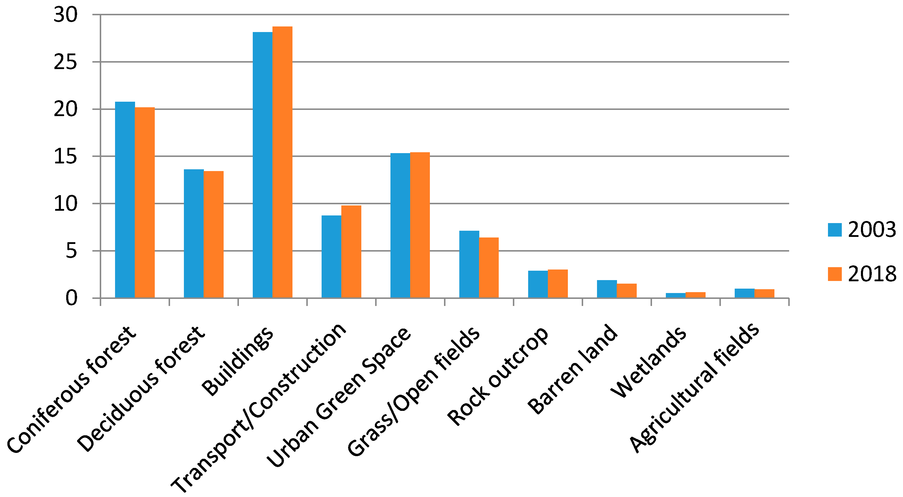
Urban areas increased and nonurban land-cover decreased by 1.7% of the city land area or roughly 327 hectares between 2003 and 2018. Urban areas increased by approximately 4% while nonurban areas decreased by 2% of their 2003 land area. Land area percentage changes for the different land-cover classes are shown in Figure 3.
In relation to their 2003 class areas, buildings increased by 2.3% or approximately 125 ha and transport/construction areas increased by 12% or roughly 202 ha. The classes most impacted by this expansion were coniferous forest, which decreased by approximately 3% or 101 ha, and grassland/open land which were reduced by 10% or 134 ha. Deciduous forest decreased by about 1% or 34 ha. The largest proportional decrease was for barren land which underwent a 19% decrease. This was largely due to the conversion of dirt sports fields to artificial grass, a type of land-cover which was classified as rock outcrop in the 2018 classification and accounts for a small percentage increase in the rock outcrop class. Wetlands and agricultural fields remained relatively stable with a slight increase for wetlands due to the later summer vegetation conditions in the 2018 imagery and a slight decrease in agricultural areas. Urban green space registered a very slight increase of less than 1%.
3.2.2. Land-Cover Change at District Level and within the Green Infrastructure
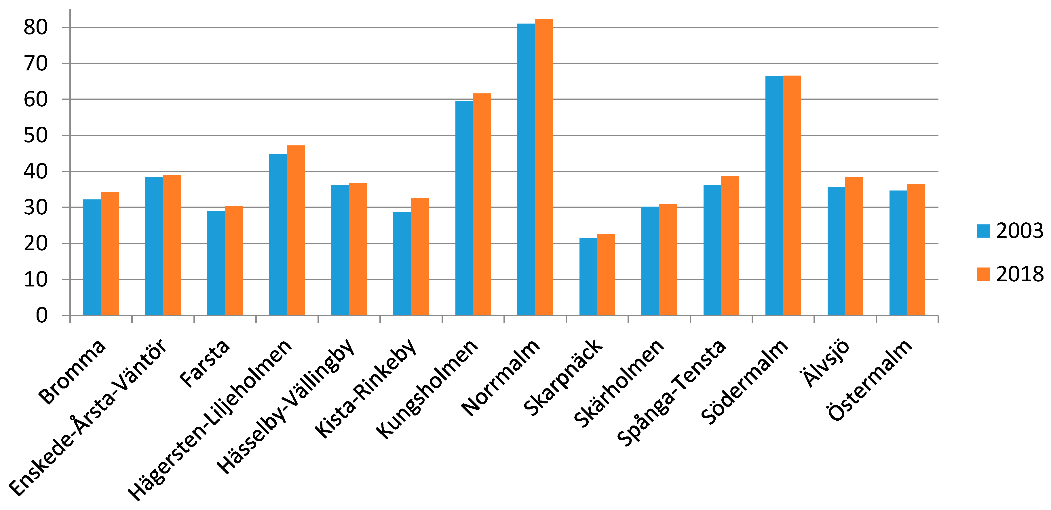
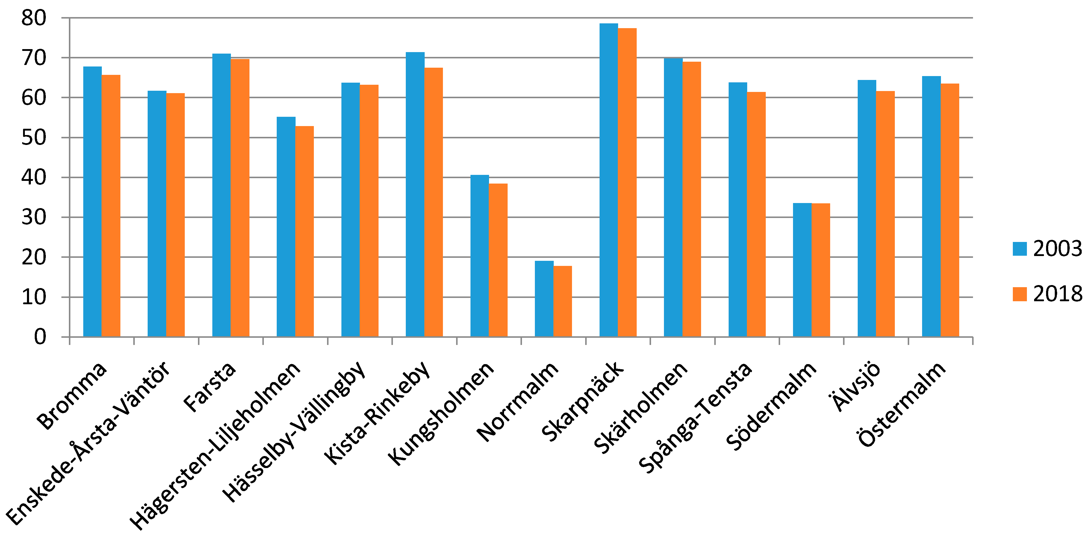
Land area percentages of urban areas (comprised of buildings and the transport/construction classes) and of green areas (comprised of deciduous/coniferous forest, urban green space, grassland/open fields, agriculture, barren land, bare rock and wetlands) for 2003 and 2018 are shown per city district in Figure 4 and Figure 5 respectively. Figure 4 displays how “urban” each district is with Kungsholmen, Norrmalm and Södermalm as the clear leaders in terms of urban areas with more than 50% urban land-cover and districts like Skarpnäck and Farsta covered by about 30% or less urban land-cover classes. The ratio of urban land-cover to green areas in the majority of the remaining districts is roughly 35/65, which indicates that on the whole Stockholm is still a very green city.
The amount of growth in hectares for urban areas and the percentage loss of green areas are listed per district in Table 3. The values are listed from largest to smallest. This listing makes clear that Södermalm experienced the least amount of change over the 15 years, while Bromma had the most hectares converted to urban land-cover and Kista-Rinkeby had the greatest percentage loss of green areas. In Kista-Rinkeby, a good deal of the green area conversion was due to the expansion of the transportation network. For Bromma, this was also true near its airport, although there were instances of building construction as well.
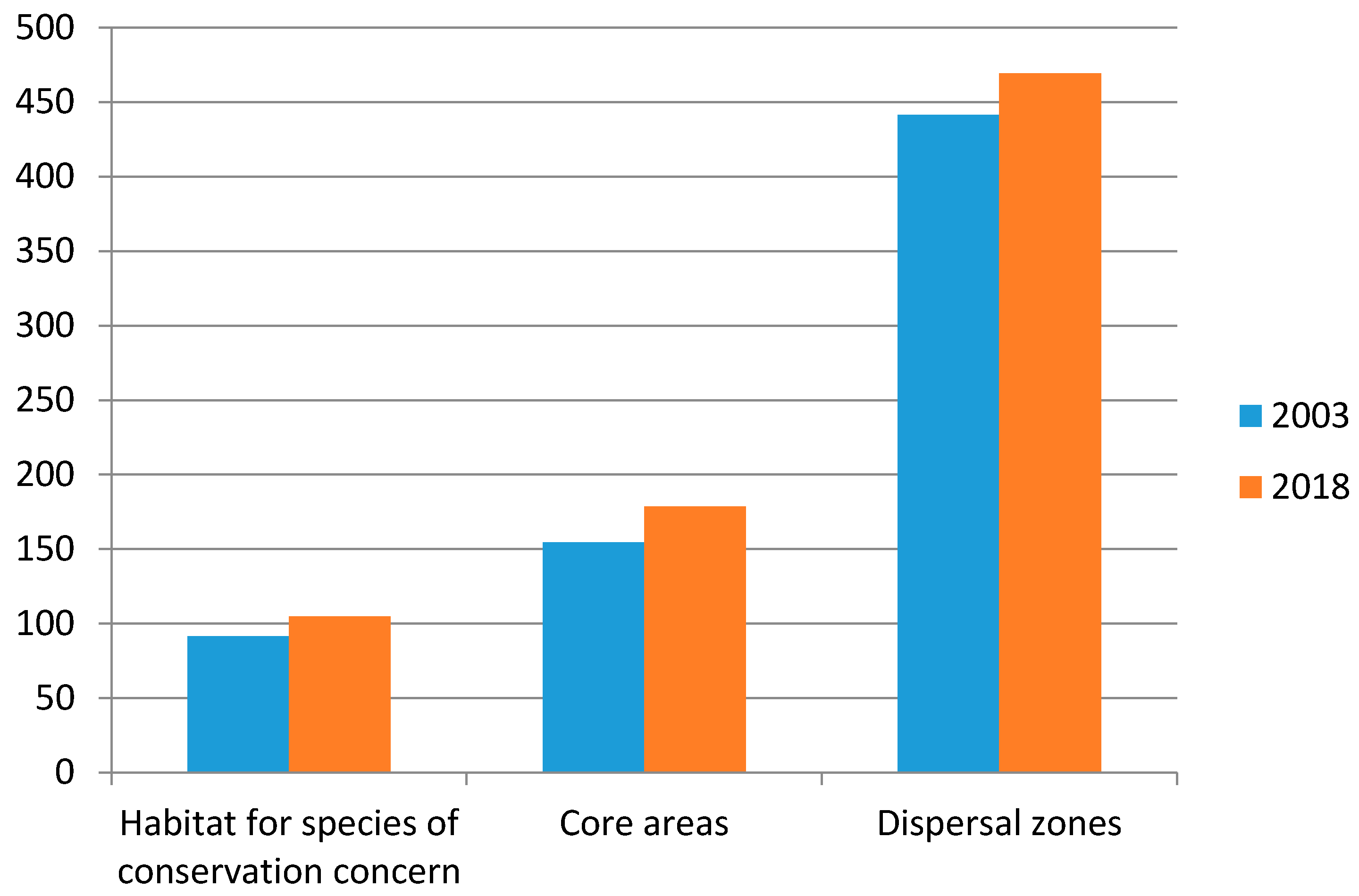
In total, there was a 9% increase in urban areas within the green infrastructure over the time period. Table 4 reports the areal and percentage increases in urban land-cover in each ecologically significant category of the green infrastructure, also shown in Figure 6.
Figure 7 illustrates the location of “newer” urban areas within the green infrastructure that appeared after 2003. These urban areas are shown in yellow while the different ecologically significant categories of the green infrastructure are highlighted in various shades of blue/purple. Roughly two-thirds of the increase within habitat for species of conservation concern was due to the construction of buildings, in areas such as Norra Sköndal (Farsta district). The other third was due to road construction and an increase in paved surfaces occurring, for example, in Solvalla near Bromma airport. Urban growth within core areas was almost exclusively due to the expansion of the transport network, most notably in the core areas located in the Kista-Rinkeby and Spånga-Tensta districts. Dispersal zones were slightly more impacted by transport network expansion, for example by the construction of new piers in the Östermalm district, than they were by new buildings of which there are examples in Beckomberga (Bromma) and Långbro/Solberga (Älvsjö).
3.2.3. Changes in Habitat Connectivity and Availability
The habitat network analysis revealed that crested tit habitat connectivity and availability decreased over the 15-year period. Table 5 shows the amount of decrease in the connectivity indices between 2003 and 2018.
The overall probability of connectivity decreased slightly for the habitat network. The decrease in ECA signifies that a single habitat patch (maximally connected) providing the same PC value as the habitat pattern in the landscape would in 2018 only be 508 ha as opposed to 530 ha in 2003. The relationship between change in overall habitat area (dA) and the change in the equivalent connected area (dECA) based on the 2003 and 2018 landscapes is dECA < dA < 0 or specifically –0.04 < –0.03 < 0 which meant that the decrease in connectivity was larger than the decrease in the area of habitat patches.
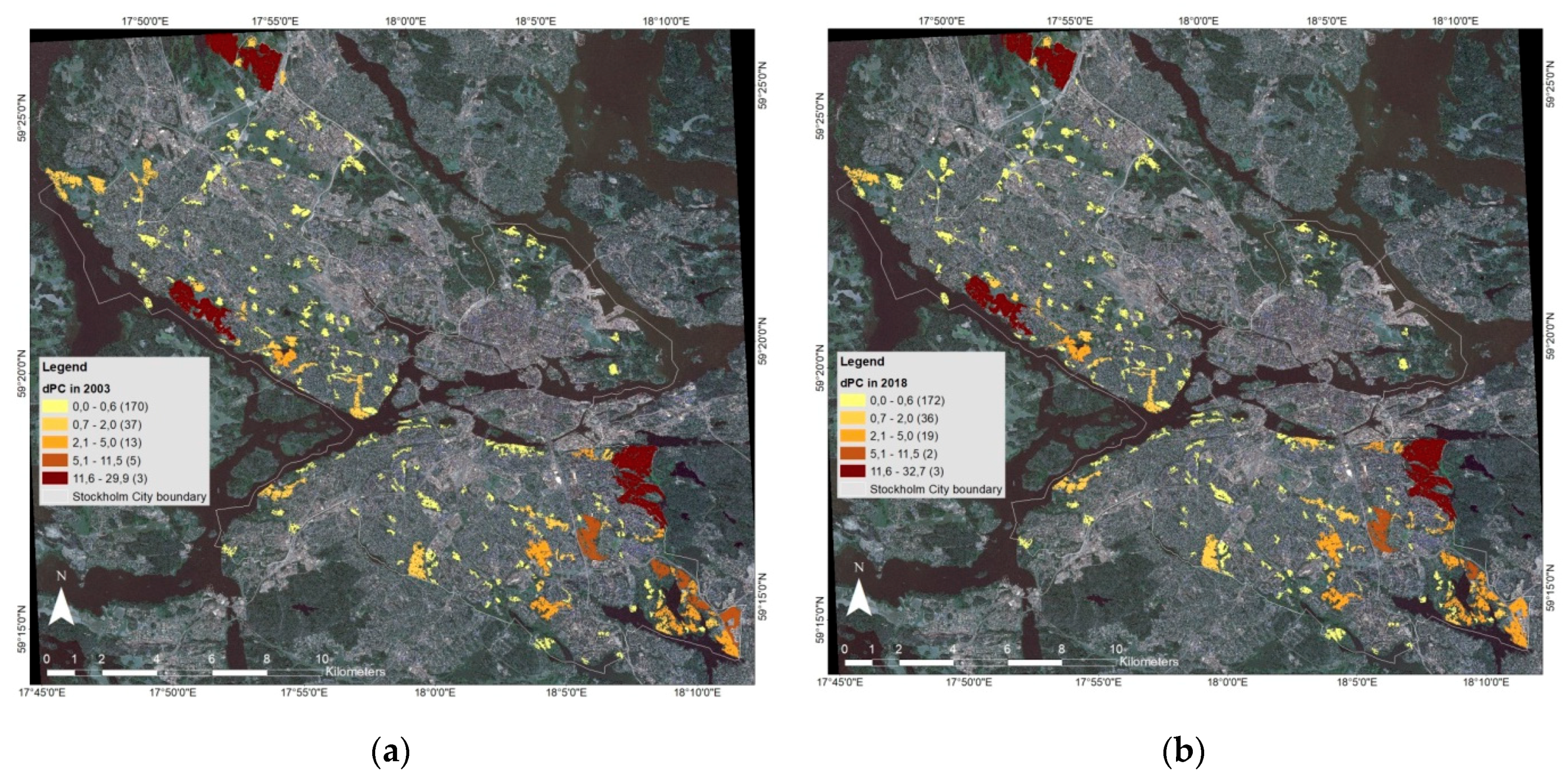
dPC values for all crested tit habitat patches in the 2003 and 2008 landscapes are illustrated in Figure 8. The darker patches are those that are most important in terms of overall connectivity. It is evident that the patch area has a significant influence on dPC value since the largest patches are also the darkest. This is indeed the case since two of the three component fractions of dPC are determined by or strongly connected to patch area: dPCintra measures internal patch connectivity (area) and dPCflux is a measure of area-weighted dispersal probabilities. Areas of high-quality habitat for the crested tit highlighted in the report by Mörtberg et al. [63] are the same as those with relatively higher dPC values in the figures, with the exception of Årstaskogen (on the waterfront in the northern part of the Enskede-Årsta-Vantör district). The number of habitat patches in each value interval is reported in parentheses and there is a slight shift towards lower dPC values in 2018.
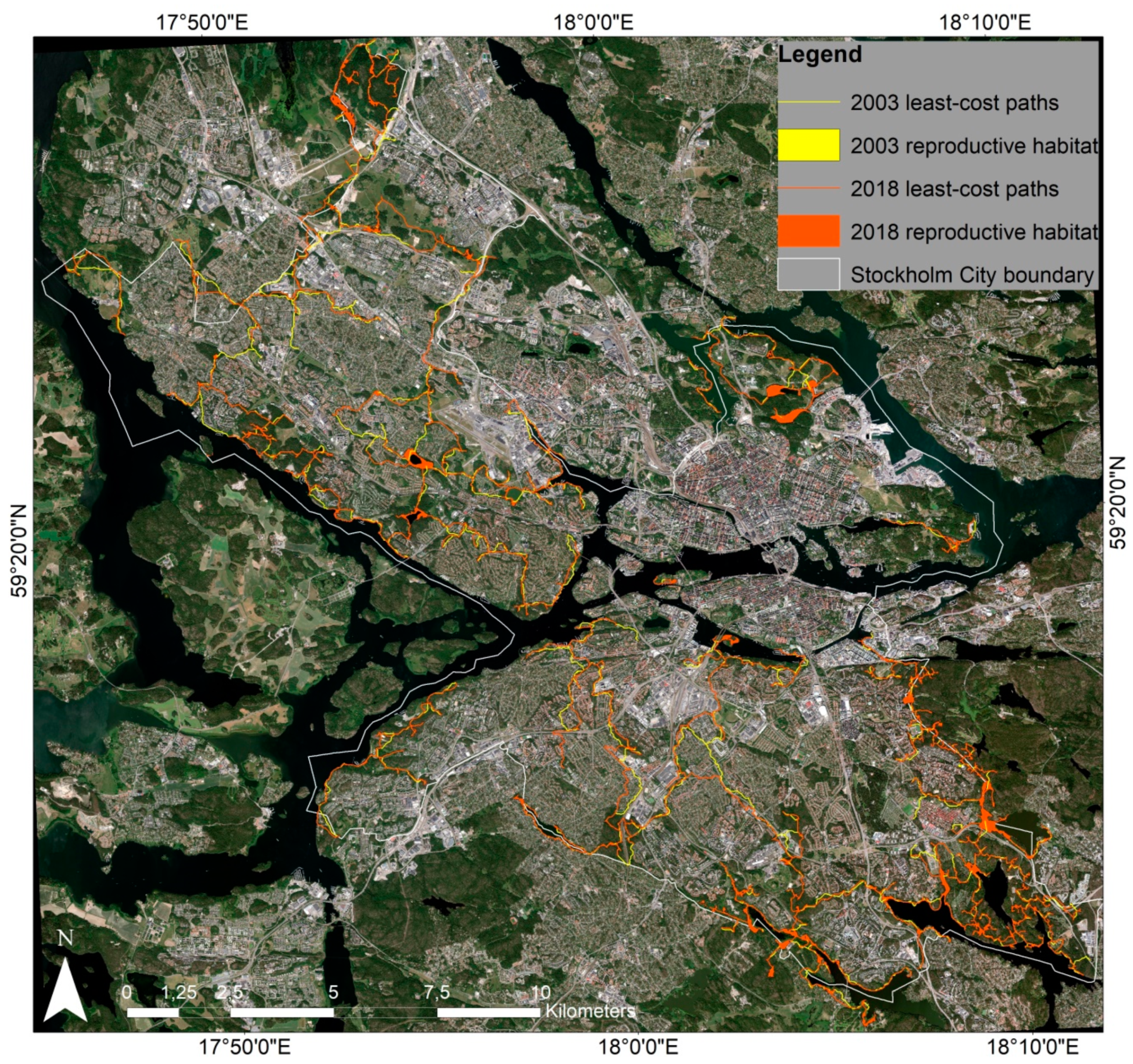
Habitat patches and least-cost pathways in the common toad habitat network for 2003 (in yellow) and 2018 (in orange) are shown in Figure 9. The habitat patches are in general small (average size 0.04 ha) but the links between them are more visible and the image makes clear that least-cost paths for toads often run through green spaces or along the outer edge of built-up areas. It also shows how certain parts of the network are isolated, notably in the northeast and southwest of Stockholm City. Very low values for PC were obtained for these networks with no noted change in the index, as displayed in Table 6. This is a limitation of PC acknowledged by Saura et al. [54] which can occur when habitat patches are small compared to the total landscape area. ECA as recommended by Saura et al. [54] can overcome this since it has areal units and will not be smaller than the largest patch in the landscape. From Table 6, we see that ECA decreased slightly signifying a drop in connectivity.
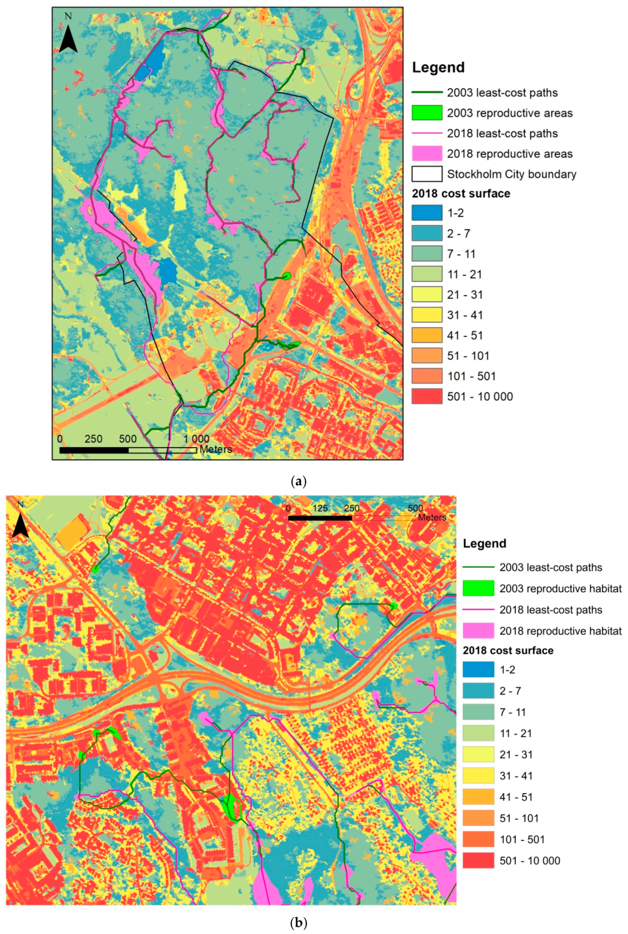
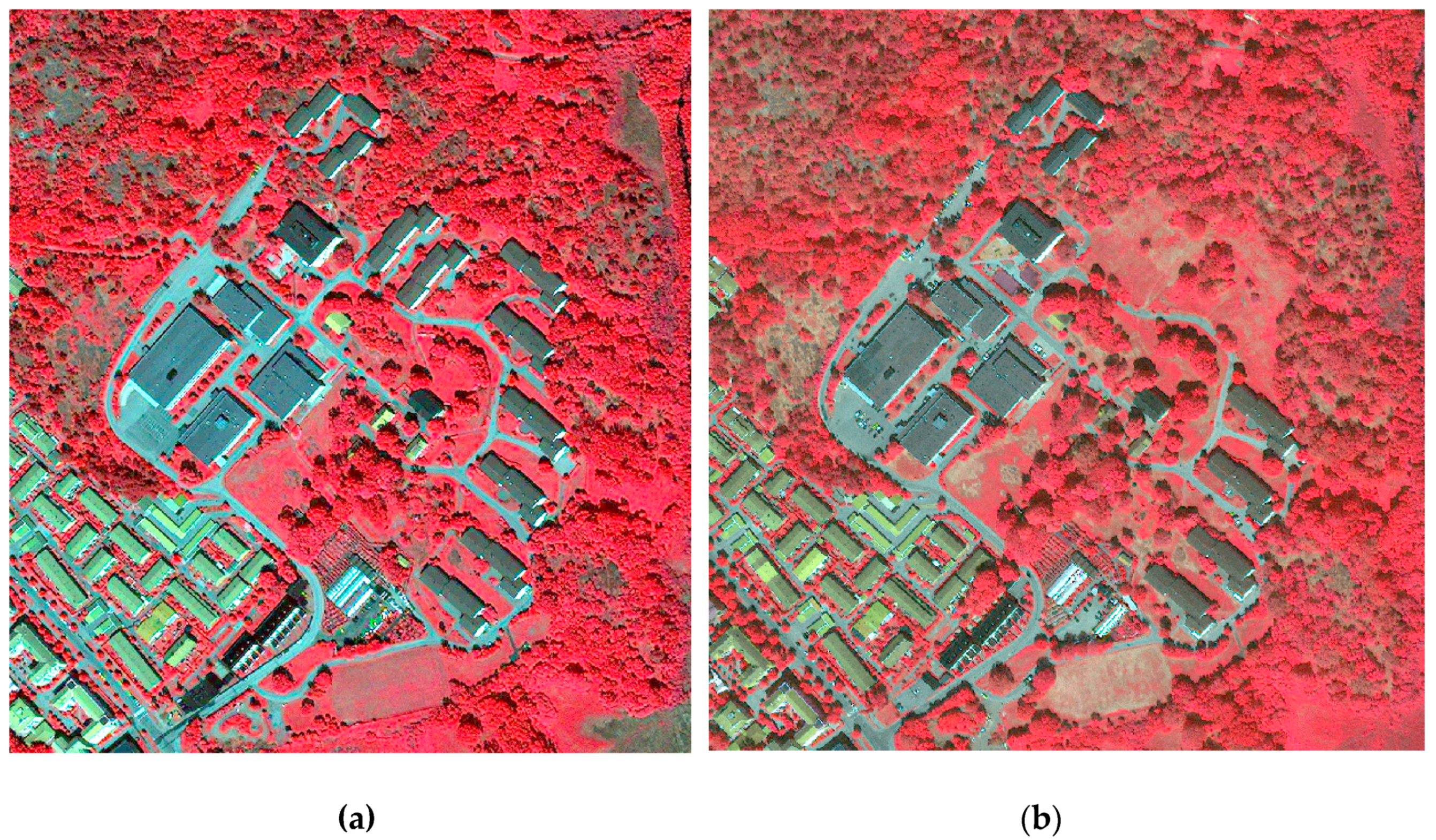
Yet dA decreased more than dECA, which indicates that the loss of habitat area was more significant between 2003 and 2018 than was the loss of connectivity in the network over the same time period. This is likely due to the fact that whole albeit small patches were lost due to the construction of new urban areas, examples of which are shown in Figure 10. Figure 10a shows an area near the Hansta Nature Reserve where 2003 patches (in green) were replaced by the expansion of transport infrastructure, while Figure 10b shows an area near Skarpnäck where 2003 patches were replaced by housing developments. For the crested tit, habitat patches were often reduced in size or divided but did not disappear altogether. The disappearance of patches and associated links in the common toad habitat meant that the network was reshaped and even to some extent consolidated, as illustrated in Figure 9 and Figure 10. Therefore most impact registered through the loss of habitat area rather than connectivity.
In order to understand more about the nature of the changes in PC and ECA values in both networks and since dPC is strongly influenced by habitat area, it is of interest to break down the metric into its component fractions and so that the value of patches as connectors or stepping stones can be assessed. Table 7 shows the percent contribution of each component of the PC index (dPCintra, dPCflux and dPCconnector) in 2003, 2018 and the interperiod change for both the crested tit and common toad habitat networks. For the crested tit habitat, dPCflux of habitat patches contributes most to connectivity in the landscape (approximately 50%) given the median distance of 200 m, followed by dPCintra (approximately 27%) and then dPCconnector (approximately 23%). By contrast for the common toad habitat network, dPCintra was the largest contributing factor to PC (approximately 93%) meaning that patches contributed most to connectivity through their size, rather than via flux (approximately 7%) or their connector role (0.2%). It is clear that the patches in the common toad habitat play a very small role as connectors or stepping stones in the network and that the loss in connectivity was due to a small decrease in flux. This differs from how connectivity changed in the crested tit habitat where the decrease was mainly due to patches playing less of a connector role in the network, although the flux was also negatively affected to a lesser degree.
Values of dPCflux in the crested tit habitat network are worth examining since this fraction is the largest contributor to overall PC and since the impact on probable connectivity was greater than the impact on habitat area as indicated by the change in ECA (Table 5). Slight decreases in value for some patches were noted in the northwest (Hässelby-Vällingby and Kista-Rinkeby districts) and southeast (southern Skarpnäck) of the city which are due to the construction of new roads resulting in fragmentation of patches in and near Hässelby-Vällingby and loss of habitat area for the two others in Kista-Rinkeby and Skarpnäck. Figure 11 shows the dPCflux values per habitat patch for each year in Hässelby-Vällingby and in southern Skarpnäck. These changes influence the value of nearby patches in the case of dPCflux since decreases in habitat area and increases in distance between patches will affect area-weighted (maximum) probabilities of dispersal. Otherwise, there is an observed consistency of values over most of the remaining landscape.
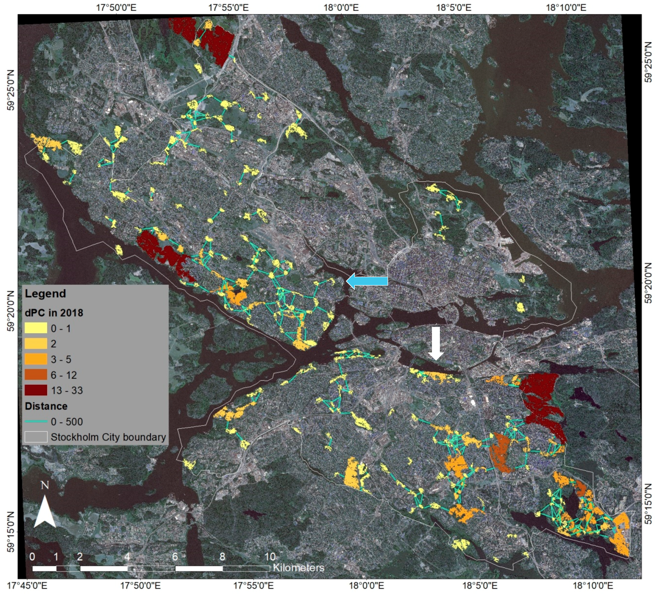
Examining the link structure from the analysis can reveal areas where restorative conservation efforts may have the most benefit. Figure 12 shows connecting links of up to 500 m in distance with dPC of crested tit habitat patches in 2018. Roughly 20% of crested tits would travel 500 m according to the median distance assumed here (200 m corresponding to probability 0.5). As an example, from this image, we can see that Årstaskogen (white arrow), one of the high-value habitat patches highlighted by Mörtberg et al. [67], appears isolated from the rest of the network. Patches that are exposed and at risk of becoming isolated also become apparent (blue arrow). The most important links for connectivity in the network based on testing patch removal (Equation (2)) were found in the areas of patches that were most well-connected, specifically in Flaten Nature Reserve in southern Skarpnäck and in Bromma. Figure 9 also reveals areas of relatively higher connectivity for the common toad, most notably again in and around Flaten Nature Reserve and Grimsta forest between Hässelby-Vällingby and Bromma.
Figure 12 also reveals why the PC values are very low in general for the crested tit habitat network. It is made up of several separate groupings of connected habitat patches. Therefore, the probability that two crested tits, if placed randomly within the network, would be able to reach one another is very low at the outset in 2003 (0.06%) and decreased very slightly (-0.01%) by 2018. Recommendations for future planning could include a focus on preserving crested tit habitat particularly in areas where connectivity is still good but where links may be exposed or at risk, such as in south-central Stockholm City and in Bromma. For the common toad, more focus may be necessary on preserving smaller habitat areas since many of the larger habitat patches are already part of the national urban park or nature reserves (such as Grimsta, Judarskogen, Kyrksjölöten, etc.). Attention and planning measures could be directed to preserving the patches that enable links between these areas.
4. Discussion
Urban growth in Stockholm City between 2003 and 2018 was modest given the increase in its population over the same time period. In relation to their 2003 class areas, buildings increased by 2.3% and transport/construction areas increased by 12% over the study time period. Coniferous forest and grasslands/open fields were the vegetated land-cover types most impacted by this urban growth, with a loss greater than 100 ha each. Expansion of the transport network negatively affected the core areas of the green infrastructure, while construction of buildings had a greater impact on habitat for species of conservation concern. Dispersal zones were affected by both types of urban growth and had the largest area converted (28 ha). Overall, there was a 9% increase in urban areas within the green infrastructure of Stockholm City. Investigation of change in habitat connectivity and availability revealed a more significant impact on probable network connectivity than habitat area for the crested tit, while by contrast common toad habitat area was more negatively affected than connectivity of the network. The impacts were due to loss, shrinkage and fragmentation of habitat patches, mainly as a result of the expansion of the transport network near the northwest and southeast outskirts of the city. Examination of the link structure of the network highlighted vulnerable or isolated parts possibly in need of strengthening or restorative efforts. Calculation of change in urban and green areas within administrative boundaries revealed that Stockholm City still has a significant proportion of green areas in comparison to urban areas, roughly 62%/38%, even if these green areas decreased slightly (–2%) as a result of urban growth over the 15-year study period.
The land-cover changes reported here are net increases in urban areas and net decreases of green areas. Yet, it is likely that there were smaller changes in the opposite direction during the study period. Indeed, during the classification process, examples of “regreening” in Stockholm City became evident. For example, an area that was previously a construction/industrial site became grassland in west Hässelby-Vällingby, buildings were removed and replaced by grassland in Nybygget in Skarpnäck and patches of barren land can be found north of Solvalla in Bromma where there were formerly buildings. There was also an example of the restoration of an edge of the green infrastructure core area in Skarpnäck as can be seen in Figure 13. Spatiotemporal land-cover analysis is effective in quantifying overall change, and classified data can be manipulated and analyzed to bring out both kinds of change. However, if an investigation requires monitoring all types of land-cover conversions, change detection techniques may be a more straightforward or practical means of highlighting changes in both directions or may be incorporated with classification techniques to provide more detailed change information, e.g., [87].
The habitat network analysis is limited to and by the city boundary, which is administrative rather than ecological in nature. Impacts on connectivity have mainly been detected on the outskirts of the study area, and for this reason, it would be interesting to shift the extent of examination to see if these impacts have more far-reaching consequences for habitat connectivity than it is possible to observe here. It should also be noted that the input parameters to the Conefor model come with some uncertainties, which will need to be further explored. In addition, the crested tit and common tit were selected as model species and a suite of representative and sensitive species will be needed to fulfill the target of representing the green infrastructure of the City. However, in this study, the purpose is to demonstrate the model development and novel linkage of remotely sensed land-cover change with habitat network analysis.
The monitoring of urban green infrastructure is an important part of sustainable urban development, supported by several policy documents, e.g., [88,89]. However, a recent study by Wellmann et al. [90] showed limited integration between ecology, remote sensing and urban planning, and that actionable knowledge and methods for planners and policymakers are rarely developed. This calls for method development of both planning tools and monitoring schemes. In fact, only a few studies have used medium- to high-resolution satellite data for urban green space mapping and change monitoring, e.g., [17,76]. The urban green space mapped, however, only included larger urban green spaces such as forest and parks while gardens and small green spaces were classified into other classes. For example, gardens were included in low-density built-up areas. Using Sentinel-2 data, Kopecká et al. [91] attempted to classify urban green space into 15 different classes including gardens and allotments. However, the reliability of their results is uncertain due to the lack of accuracy assessment. The highly heterogeneous urban landscape with a complex mix of impervious surfaces and vegetation requires mapping at a finer scale. As a result, very high-resolution satellite data have been exploited to classify urban green spaces in Europe and around the world, e.g., [28,29,92,93]. These studies, however, mainly focused on methods to map urban green space. No studies were found to utilize their urban green space result to further develop planning tools and monitoring schemes. This research is the first attempt to integrate high-resolution data and ecological tools for urban green space monitoring and environmental impact analysis to support planning actions. The spatiotemporal analysis of the green infrastructure and habitat network analysis could play a useful role in the local planning authority’s environmental assessment and monitoring.
Stockholm City as well as Stockholm Region have developed a formal policy for biodiversity management and have been using several planning tools including green infrastructure. Consequently, a viable green infrastructure is one of the goals for urban development according to the comprehensive plan of Stockholm City [9]. Stockholm City’s proposed biodiversity and related ecosystem service monitoring program [89] relies in part on locally conducted species inventories and also has planned measures such as habitat network analysis and spatiotemporal assessment of change in mapped biotopes. It mentions possible specific response measures such as installation and restoration of amphibian ponds. Results of the common toad network analysis revealed modifications to the network and provided information on where habitat has been lost and where reinstallation might be most beneficial to the network. In this way, status and change information from habitat network analysis could inform and help target restorative or conservation measures. However, there is a need for further development of these tools including the underlying habitat network analyses, and monitoring frameworks and practices. The analyses performed here are examples of practical development and implementation of habitat network and green infrastructure monitoring. The habitat networks need to be expanded to include main biodiversity components and ecosystem services, and be integrated with smart monitoring schemes to follow the changes. Lastly, the state and change of prioritized habitat networks need to be integrated into urban planning practice in order to reach sustainable urban development.
5. Conclusions
In this research, object-oriented SVM classifications of WorldView-2 and QuickBird-2 satellite data were used to investigate urban expansion in Stockholm City between 2003 and 2018 and the resulting environmental impacts on green areas and green infrastructure. The classifications had similar high accuracies (kappa: 0.90 and 0.92). Quantitative analysis based on the classifications has estimated broad changes, i.e., land-cover change at city landscape, down to detailed impacts, i.e., changes in terms of habitat connectivity and availability of individual habitat patches, by examining different analysis levels in Stockholm City. These are in relation to urban growth within city districts, green infrastructure and by evaluating changes in habitat connectivity and availability for selected sensitive species in the Stockholm City context. This information provides insight into where and relatively how much change occurred in different areas within the city and can inform decisions about where future urban growth should or can take place.
Between 2003 and 2018, urban areas increased and nonurban land-cover decreased by 1.7% of the city landscape area or 327 ha. Green areas decreased by 2% while urban areas increased by 4% in comparison with their 2003 aerial extent. An increase in the transport network, paved surfaces and construction sites made up 60% of the urban growth that occurred in Stockholm City between 2003 and 2018, while the remaining 40% was a net increase in buildings. This growth affected the city’s green infrastructure: core areas and dispersal zones were mainly impacted by the expansion of transport and construction sites while habitat for species of conservation concern was more affected by the addition of new buildings. Expansion of the transport network and construction sites also negatively influenced connectivity in the crested tit habitat network through patch shrinkage and fragmentation mainly on the outskirts of the city. The common toad habitat network was more affected by an outright loss of patches due to the expansion of both residential areas and transport infrastructure. A continually updated spatiotemporal analysis of the green infrastructure and habitat network analysis could play a useful role in future environmental assessment by planning authorities and increase the effectiveness of restorative efforts and resources for biodiversity conservation in cities.
Author Contributions
Conceptualization: Y.B., D.F. and U.M.; methodology: D.F., Y.B. and U.M.; validation: D.F.; formal analysis: D.F.; investigation: D.F.; resources: Y.B.; data curation: D.F.; writing—original draft preparation: D.F.; writing—review and editing: Y.B. and U.M.; visualization: D.F.; supervision: Y.B. and U.M.; project administration: Y.B. and D.F.; funding acquisition: Y.B. All authors have read and agreed to the published version of the manuscript.
Funding
This research was funded by KTH Digital Futures and the European Space Agency, Contract No. 4000122145/18/I-NB.
Acknowledgments
This research is part of the project ‘Earth Observation for Smart Cities and Sustainable Urbanization’ (European Lead PI: Yifang Ban) within the European Space Agency (ESA) and Chinese Ministry of Science and Technology (MOST) Dragon 4 program. Satellite images were provided courtesy of the DigitalGlobe Foundation. The authors are grateful to the Stockholm City Environmental Management Department (Miljöförvaltningen) for provision of the Stockholm City green infrastructure geographic datasets.
Conflicts of Interest
The authors declare no conflict of interest.
Appendix A

Table A1.
Crested tit and common toad species criteria according to Mörtberg et al. [66,67] and corresponding parameters used in the present study.
| Criteria | Reference | Parameter Used | |
|---|---|---|---|
| Crested Tit | |||
| Habitat preference | Mature and old pine and spruce forests | [77,94] | Land-cover for habitat patches: coniferous forest |
| Nesting areal requirement | Roughly 2–3 ha | [95] | Patch size minimum: 2 ha |
| Dispersal distance | Several kilometers within habitat but reluctant to cross open spaces | [78,79,80] | Assumed median dispersal/movement distance in urban environment: 200 m |
| Common Toad | |||
| Dispersal distance | Up to 2 km over optimal land-cover but only a few meters over unsuitable land-cover (Table A3) | [96,97,98,99] | Assumed maximum dispersal/movement distance in urban environment: 2 km |
Table A2.
Resource profile for the common toad according to Mörtberg et al. [66].
Table A2.
Resource profile for the common toad according to Mörtberg et al. [66].
| Habitat | Quality | Biotope/Land-Cover |
|---|---|---|
| Reproductive habitat | Optimal | Wetlands, water with vegetation, streams, water-filled ditches |
| Summer habitat | Optimal | Deciduous forest, mixed forest, moist grassland |
| Suboptimal | Low-density built-up areas with trees/bushes, older coniferous forest, managed grassland | |
| Marginal | Low-density built-up areas without vegetation, young coniferous/mixed forest, heavily managed grassland, agricultural areas | |
| Winter habitat | Optimal | Deciduous forest |
| Suboptimal | Mixed forest, grassland with trees/bushes, low-density built-up areas with trees/bushes | |
| Marginal | Coniferous forest |
Table A3.
Dispersal profile for the common toad according to Mörtberg et al. [66]
Table A3.
Dispersal profile for the common toad according to Mörtberg et al. [66]
| Quality for Dispersal | Biotope/Land-Cover |
|---|---|
| Optimal | Deciduous forest, older coniferous/mixed forest, moist grassland |
| Medium | Low-density built-up areas with trees/bushes, young coniferous/mixed forest |
| Unsuitable | Built-up areas with sealed surfaces, including roads, low-density built-up areas without or with heavily managed vegetation, clear-cut areas |
| Barrier | Buildings, sound berms, steep slopes |
References
- Aronson, M.; LaSorte, F.A.; Nilon, C.H.; Katti, M.; Goddard, M.A.; Lepczyk, C.A.; Warren, P.S.; Williams, W.P.S.; Cilliers, S.; Clarkson, B.; et al. A global analysis of the impacts of urbanization on bird and plant diversity reveals key anthropogenic drivers. Proc. Biol. Sci. 2014, 281, 20133330. [Google Scholar] [CrossRef]
- European Commission. Green Infrastructure (GI)—Enhancing Europe’s Natural Capital. Communication COM 249. 2013. Available online: https://eur-lex.europa.eu/legal-content/EN/TXT/?uri=CELEX:52013DC0249 (accessed on 20 July 2020).
- European Commission. EU Biodiversity Strategy for 2030: Bringing Nature Back into Our Lives. Communication COM 380. 2020. Available online: https://eur-lex.europa.eu/resource.html?uri=cellar:a3c806a6-9ab3-11ea-9d2d-01aa75ed71a1.0001.02/DOC_1&format=PDF (accessed on 3 September 2020).
- Swedish Environmental Protection Agency. Regionala Handlingsplaner för Grön Infrastruktur och Prioritering av Naturvårdsinsatser [Regional Action Plans for Green Infrastructure and Priorization of Nature Conservation Efforts]. 2017. Available online: https://www.naturvardsverket.se/upload/stod-i-miljoarbetet/vagledning/samhallsplanering/Vagledning-GI-naturvardsprioriteringar.pdf (accessed on 20 July 2020). (In Swedish)
- Stockholm County Administrative Board. Grön infrastruktur—Regional Handlingsplan för Stockholms län [Green infrastructure—Regional Action Plan for Stockholm County]. Report December 2019. Available online: https://www.lansstyrelsen.se/download/18.35db062616a5352a22a21fa1/1560332365801/R2019-12%20Gr%C3%B6n%20infrastruktur-Handlingsplan.pdf (accessed on 20 July 2020). (In Swedish)
- Tzoulas, K.; Korpela, K.; Venn, S.; Yli-Pelkonen, V.; Kaźmierczak, A.; Niemela, J.; James, P. Promoting ecosystem and human health in urban areas using Green Infrastructure: A literature review. Landsc. Urban Plan. 2007, 81, 167–178. [Google Scholar] [CrossRef] [Green Version]
- Pauleit, S.; Ambrose-Oji, B.; Andersson, E.; Anton, B.; Buijs, A.; Haase, D.; Elands, B.; Hansen, R.; Kowarik, I.; Kronenberg, J.; et al. Advancing urban green infrastructure in Europe: Outcomes and reflections from the GREEN SURGE project. Urban For. Urban Green. 2019, 40, 4–16. [Google Scholar] [CrossRef]
- Mörtberg, U.; Zetterberg, A.; Brokking Balfors, B. Urban landscapes in transition: Lessons from integrating biodiversity and habitat modelling in planning. J. Environ. Assess. Policy Manag. 2012, 14, 1250002. [Google Scholar] [CrossRef]
- Stockholm City. Översiktsplan för Stockholms stad [Comprehensive plan for the City of Stockholm]. 2018. Available online: https://vaxer.stockholm/globalassets/tema/oversiktsplanen/uppdatering-av-op/godkannade-op/oversiktsplan-for-stockholms-stad-godkannandehandling.pdf (accessed on 20 July 2020). (In Swedish)
- Stockholm City. Hållbar mark-och Vattenanvändning [Sustainable Land and Water Use]. 2019. Available online: http://miljobarometern.stockholm.se/miljomal/miljoprogram-2016-2019/hallbar-mark-och-vattenanvandning/ (accessed on 20 July 2020). (In Swedish)
- Stadsbyggnadskontoret Stockholm city building office. In Proceedings of the Communication within EO&AI4ChangeDetection Project Meeting, Stockholm, Sweden, 10 October 2019.
- Herold, M.; Couclelis, H.; Clarke, K.C. The role of spatial metrics in the analysis and modeling of urban land use change. Comput. Environ. Urban Syst. 2005, 29, 369–399. [Google Scholar] [CrossRef]
- Gamba, P.; Herold, M. Global Mapping of Human Settlement: Experiences, Datasets, and Prospects; CRC Press: Boca Raton, FL, USA, 2009. [Google Scholar]
- Furberg, D.; Ban, Y. Satellite monitoring of urban sprawl and assessment of its potential environmental impact in the greater toronto area between 1985 and 2005. Environ. Manag. 2012, 50, 1068–1088. [Google Scholar] [CrossRef]
- Wang, L.; Li, C.; Ying, Q.; Cheng, X.; Wang, X.; Li, X.; Hu, L.; Liang, L.; Yu, L.; Huang, H.; et al. China’s urban expansion from 1990 to 2010 determined with satellite remote sensing. Chin. Sci. Bull. 2012, 57, 2802–2812. [Google Scholar] [CrossRef] [Green Version]
- Liu, T.; Yang, X. Monitoring land changes in an urban area using satellite imagery, GIS and landscape metrics. Appl. Geogr. 2015, 56, 42–54. [Google Scholar] [CrossRef]
- Haas, J.; Ban, Y. Urban land cover and ecosystem service changes based on sentinel-2a msi and landsat tm data. IEEE J. Sel. Top. Appl. Earth Obs. Remote Sens. 2018, 11, 485–497. [Google Scholar] [CrossRef]
- Ban, Y.; Hu, H.; Rangel, I.M. Fusion of Quickbird MS and RADARSAT SAR data for urban land-cover mapping: Object-based and knowledge-based approach. Int. J. Remote Sens. 2010, 31, 1391–1410. [Google Scholar] [CrossRef]
- Myint, S.W.; Gober, P.; Brazel, A.; Grossman-Clarke, S.; Weng, Q. Per-pixel vs. object-based classification of urban land cover extraction using high spatial resolution imagery. Remote Sens. Environ. 2011, 115, 1145–1161. [Google Scholar] [CrossRef]
- Ma, L.; Li, M.; Ma, X.; Cheng, L.; Du, P.; Liu, Y. A review of supervised object-based land-cover image classification. ISPRS J. Photogramm. Remote Sens. 2017, 130, 277–293. [Google Scholar] [CrossRef]
- Momeni, R.; Aplin, P.; Boyd, D.S. Mapping complex urban land cover from spaceborne imagery: The influence of spatial resolution, spectral band set and classification approach. Remote Sens. 2016, 8, 88. [Google Scholar] [CrossRef] [Green Version]
- Shackelford, A.K.; Davis, C.H. A combined fuzzy pixel-based and object-based approach for classification of high-resolution multispectral data over urban areas. IEEE Trans. Geosci. Remote Sens. 2003, 41, 2354–2363. [Google Scholar] [CrossRef] [Green Version]
- Haas, J.; Ban, Y. Mapping and monitoring urban ecosystem services using multitemporal high-resolution satellite data. IEEE J. Sel. Top. Appl. Earth Obs. Remote Sens. 2017, 10, 669–680. [Google Scholar] [CrossRef]
- Mugiraneza, T.; Nascetti, A.; Ban, Y. WorldView-2 data for hierarchical object-based urban land cover classification in kigali: Integrating rule-based approach with urban density and greenness indices. Remote Sens. 2019, 11, 2128. [Google Scholar] [CrossRef] [Green Version]
- Mutuku, F.M.; Bayoh, M.N.; Hightower, A.W.; Vulule, J.M.; Gimnig, J.E.; Mueke, J.M.; Amimo, F.A.; Walker, E.D. A supervised land cover classification of a western Kenya lowland endemic for human malaria: Associations of land cover with larval Anopheles habitats. Int. J. Health Geogr. 2009, 8, 19. [Google Scholar] [CrossRef] [Green Version]
- Recio, M.R.; Mathieu, R.; Hall, G.B.; Moore, A.B.; Seddon, P.J. Landscape resource mapping for wildlife research using very high resolution satellite imagery. Methods Ecol. Evol. 2013, 4, 982–992. [Google Scholar] [CrossRef]
- Sawaya, K.E.; Olmanson, L.G.; Heinert, N.J.; Brezonik, P.L.; Bauer, M.E. Extending satellite remote sensing to local scales: Land and water resource monitoring using high-resolution imagery. Remote Sens. Environ. 2003, 88, 144–156. [Google Scholar] [CrossRef]
- Mathieu, R.; Freeman, C.; Aryal, J. Mapping private gardens in urban areas using object-oriented techniques and very high-resolution satellite imagery. Landsc. Urban Plan. 2007, 81, 179–192. [Google Scholar] [CrossRef]
- Lang, S.; Blaschke, T.; Kothencz, G.; Hölbling, D. Urban green mapping and valuation. In Urban Remote Sensing, 2nd ed.; Weng, Q., Quattrochi, D., Gamba, P.E., Eds.; CRC Press: Boca Raton, FL, USA, 2018; pp. 287–309. [Google Scholar]
- Lakes, T.; Kim, H.O. The urban environmental indicator “Biotope Area Ratio”—an enhanced approach to assess and manage the urban ecosystem services using high resolution remote-sensing. Ecol. Indic. 2012, 13, 93–103. [Google Scholar] [CrossRef]
- Turner, W.; Rondinini, C.; Pettorelli, N.; Mora, B.; Leidner, A.K.; Szantoi, Z.; Buchanan, G.; Dech, S.; Dwyer, J.; Herold, M.; et al. Free and open-access satellite data are key to biodiversity conservation. Biol. Conserv. 2015, 182, 173–176. [Google Scholar] [CrossRef] [Green Version]
- Pettorelli, N.; Laurance, W.F.; O’Brien, T.G.; Wegmann, M.; Nagendra, H.; Turner, W. Satellite remote sensing for applied ecologists: Opportunities and challenges. J. Appl. Ecol. 2014, 51, 839–848. [Google Scholar] [CrossRef]
- Pettorelli, N.; Safi, K.; Turner, W. Satellite remote sensing, biodiversity research and conservation of the future. Philos. Trans. R. Soc. B 2014, 369, 20130190. [Google Scholar] [CrossRef] [PubMed]
- Mairota, P.; Cafarelli, B.; Didham, R.K.; Lovergine, F.P.; Lucas, R.M.; Nagendra, H.; Rocchini, D.; Tarantino, C. Challenges and opportunities in harnessing satellite remote-sensing for biodiversity monitoring. Ecol. Inform. 2015, 30, 207–214. [Google Scholar] [CrossRef]
- Boyle, S.A.; Kennedy, C.M.; Torres, J.; Colman, K.; Pérez-Estigarribia, P.E.; Noé, U. High-resolution satellite imagery is an important yet underutilized resource in conservation biology. PLoS ONE 2014, 9, e86908. [Google Scholar] [CrossRef]
- Nagendra, H.; Lucas, R.; Honrado, J.P.; Jongman, R.H.; Tarantino, C.; Adamo, M.; Mairota, P. Remote sensing for conservation monitoring: Assessing protected areas, habitat extent, habitat condition, species diversity, and threats. Ecol. Indic. 2013, 33, 45–59. [Google Scholar] [CrossRef]
- Löfvenhaft, K.; Runborg, S.; Sjögren-Gulve, P. Biotope patterns and amphibian distribution as assessment tools in urban landscape planning. Landsc. Urban Plan. 2004, 68, 403–427. [Google Scholar] [CrossRef]
- Hartfield, K.A.; Landau, K.I.; Van Leeuwen, W.J. Fusion of high resolution aerial multispectral and LiDAR data: Land cover in the context of urban mosquito habitat. Remote Sens. 2011, 3, 2364–2383. [Google Scholar] [CrossRef] [Green Version]
- Cleve, C.; Kelly, M.; Kearns, F.R.; Moritz, M. Classification of the wildland–urban interface: A comparison of pixel-and object-based classifications using high-resolution aerial photography. Comp. Environ. Urban Syst. 2008, 32, 317–326. [Google Scholar] [CrossRef]
- Agarwal, S.; Vailshery, L.; Jaganmohan, M.; Nagendra, H. Mapping urban tree species using very high resolution satellite imagery: Comparing pixel-based and object-based approaches. ISPRS Int. J. Geo Inf. 2013, 2, 220–236. [Google Scholar] [CrossRef]
- Qian, Y.; Zhou, W.; Yan, J.; Li, W.; Han, L. Comparing machine learning classifiers for object-based land cover classification using very high resolution imagery. Remote Sens. 2015, 7, 153–168. [Google Scholar] [CrossRef]
- Pande-Chhetri, R.; Abd-Elrahman, A.; Liu, T.; Morton, J.; Wilhelm, V.L. Object-based classification of wetland vegetation using very high-resolution unmanned air system imagery. Eur. J. Remote Sens. 2017, 50, 564–576. [Google Scholar] [CrossRef] [Green Version]
- Fahrig, L. Effects of habitat fragmentation on biodiversity. Annu. Rev. Ecol. Evol. Syst. 2003, 34, 487–515. [Google Scholar] [CrossRef] [Green Version]
- St-Laurent, M.-H.; Dussault, C.; Ferron, J.; Gagnon, R. Dissecting habitat loss and fragmentation effects following logging in boreal forest: Conservation perspectives from landscape simulations. Biol. Conserv. 2009, 142, 2240–2249. [Google Scholar] [CrossRef]
- Hanski, I. Metapopulation models. In Encyclopedia of Ecology; Jorgensen, S.E., Fath, B.D., Eds.; Elsevier: Amsterdam, The Netherlands, 2008; pp. 2318–2325. [Google Scholar]
- Urban, D.; Keitt, T. Landscape connectivity: A graph-theoretic perspective. Ecology 2001, 82, 1205–1218. [Google Scholar] [CrossRef]
- Estrada, E.; Bodin, Ö. Using network centrality measures to manage landscape connectivity. Ecol. Appl. 2008, 18, 1810–1825. [Google Scholar] [CrossRef] [Green Version]
- Bodin, Ö.; Zetterberg, A. MatrixGreen: Landscape Ecological Network Analysis Tool–User Manual. Paper V in Connecting the Dots. Doctoral Thesis, KTH Royal Institute of Technology, Stockholm, Sweden, 2011. [Google Scholar]
- Zetterberg, A.; Mörtberg, U.M.; Balfors, B. Making graph theory operational for landscape ecological assessments, planning, and design. Landsc. Urban Plan. 2010, 95, 181–191. [Google Scholar] [CrossRef]
- Saunders, M.I.; Brown, C.J.; Foley, M.M.; Febria, C.M.; Albright, R.; Mehling, M.G.; Kavanaugh, M.T.; Burfeind, D.D. Human impacts on connectivity in marine and freshwater ecosystems assessed using graph theory: A review. Mar. Freshw. Res. 2016, 67, 277–290. [Google Scholar] [CrossRef] [Green Version]
- Huang, Y.; Huang, J.L.; Liao, T.J.; Liang, X.; Tian, H. Simulating urban expansion and its impact on functional connectivity in the Three Gorges Reservoir Area. Sci. Total Environ. 2018, 643, 1553–1561. [Google Scholar] [CrossRef]
- Saura, S.; Pascual-Hortal, L. A new habitat availability index to integrate connectivity in landscape conservation planning: Comparison with existing indices and application to a case study. Landsc. Urban Plan. 2007, 83, 91–103. [Google Scholar] [CrossRef]
- Saura, S.; Rubio, L. A common currency for the different ways in which patches and links can contribute to habitat availability and connectivity in the landscape. Ecography 2010, 33, 523–537. [Google Scholar] [CrossRef]
- Saura, S.; Estreguil, C.; Mouton, C.; Rodríguez-Freire, M. Network analysis to assess landscape connectivity trends: Application to European forests (1990–2000). Ecol. Indic. 2011, 11, 407–416. [Google Scholar] [CrossRef]
- Pérez-Hernández, C.G.; Vergara, P.M.; Saura, S.; Hernández, J. Do corridors promote connectivity for bird-dispersed trees? The case of Persea lingue in Chilean fragmented landscapes. Landsc. Ecol. 2015, 30, 77–90. [Google Scholar] [CrossRef]
- Herrera, L.P.; Sabatino, M.C.; Jaimes, F.R.; Saura, S. Landscape connectivity and the role of small habitat patches as stepping stones: An assessment of the grassland biome in South America. Biodivers. Conserv. 2017, 26, 3465–3479. [Google Scholar] [CrossRef]
- Diniz, M.F.; Machado, R.B.; Bispo, A.A.; Brito, D. Identifying key sites for connecting jaguar populations in the Brazilian Atlantic Forest. Anim. Conserv. 2018, 21, 201–210. [Google Scholar] [CrossRef]
- Bolliger, J.; Silbernagel, J. Contribution of connectivity assessments to Green Infrastructure (GI). ISPRS Int. J. Geo Inf. 2020, 9, 212. [Google Scholar] [CrossRef] [Green Version]
- Zhang, Z.; Meerow, S.; Newell, J.P.; Lindquist, M. Enhancing landscape connectivity through multifunctional green infrastructure corridor modeling and design. Urban For. Urban Green. 2019, 38, 305–317. [Google Scholar] [CrossRef]
- Perkl, R.; Norman, L.M.; Mitchell, D.; Feller, M.; Smith, G.; Wilson, N.R. Urban growth and landscape connectivity threats assessment at Saguaro National Park, Arizona, USA. J. Land Use Sci. 2018, 13, 102–117. [Google Scholar] [CrossRef]
- Nor, A.N.M.; Corstanje, R.; Harris, J.A.; Grafius, D.R.; Siriwardena, G.M. Ecological connectivity networks in rapidly expanding cities. Heliyon 2017, 3, e00325. [Google Scholar] [CrossRef] [Green Version]
- Stockholm City. Statistical Year-Book of Stockholm 2018; Stockholm City: Stockholm, Sweden, 2018. Available online: https://start.stockholm/globalassets/start/om-stockholms-stad/utredningar-statistik-och-fakta/statistik/arsbok/arsbok_2018.pdf (accessed on 20 July 2020).
- Growth and Regional Planning Administration—GRPA (Tillväxt- och Regionplaneförvaltningen). Regional utvecklingsplan för Stockholmsregionen RUFS 2050 [Regional Development Plan for the Stockholm Region RUFS 2050]. Stockholm County Council. 2018. Available online: http://rufs.se/globalassets/e.-rufs-2050/rufs_regional_utvecklingsplan_for_stockholmsregionen_2050_tillganglig.pdf (accessed on 20 July 2020). (In Swedish).
- Stockholm City Environmental Management Department (Miljöförvaltningen, Stockholms stad). Stockholms Ekologiska Infrastruktur—Bakgrund och Beskrivning av Databas och Karta. [Stockholm’s ecological infrastructure—Background and description of the database and map.]. Version 14 February 2014. Available online: http://miljobarometern.stockholm.se/content/docs/mp15/4/ESBO_Bed%C3%B6mningsgrunder.pdf (accessed on 20 July 2020). (In Swedish)
- Gothnier, M.; Hjorth, G.; Östergård, S. Rapport från ArtArken [Report from the Species Ark]. Stockholms artdata-arkiv. Miljöförvaltningen: Stockholm, Sweden, 1999. Available online: http://miljobarometern.stockholm.se/content/docs/tema/natur/Rapport%20fr%C3%A5n%20ArtArken1999%20publ.pdf (accessed on 20 July 2020). (In Swedish)
- Mörtberg, U.; Zetterberg, A.; Gontier, M. Landskapsekologisk analys i Stockholms stad: Metodutveckling med groddjur som exempel [Landscape Ecological Analysis i Stockholm City: Method Development with Amphibians as an Example]; Miljöförvaltningen: Stockholm, Sweden, 2006; Available online: http://miljobarometern.stockholm.se/content/docs/tema/natur/Habitatverktyg_groddjur_2008.pdf (accessed on 20 July 2020). (In Swedish)
- Mörtberg, U.; Zetterberg, A.; Gontier, M. Landskapsekologisk Analys i Stockholms stad: Habitatnätverk för Eklevande Arter och Barrskogsarter [Landscape Ecological Analysis i Stockholm City: Habitat Networks for Oak-Dependent Species and Coniferous Forest Species]; Miljöförvaltningen: Stockholm, Sweden, 2007. Available online: http://miljobarometern.stockholm.se/content/docs/tema/natur/Habitatverktyg_ek_barrskogsarter_2008.pdf (accessed on 20 July 2020). (In Swedish)
- Zhang, Y. 2008. Pan-sharpening for improved information extraction. In Advances in Photogrammetry, Remote Sensing and Spatial Information Sciences; Li, Z., Chen, J., Baltsavias, E., Eds.; CRC Press: Boca Raton, FL, USA, 2008; Volume 7, Chapter 14; pp. 185–203. [Google Scholar]
- Zhang, Y. Problems in the fusion of commercial high-resolution satellite as well as Landsat 7 images and initial solutions. Int. Arch. Photogramm. Remote Sens. Spat. Inf. Sci. 2002, 34, 587–592. [Google Scholar]
- DigitalGlobe. QuickBird Datasheet. 2014. Available online: https://dgv4-cms-production.s3.amazonaws.com/uploads/document/file/131/QuickBird-DS-QB-Prod.pdf (accessed on 20 July 2020).
- DigitalGlobe. WorldView-2 Datasheet. 2016. Available online: https://dgv4-cms-production.s3.amazonaws.com/uploads/document/file/130/WorldView2-DS-WV2-rev2.pdf (accessed on 20 July 2020).
- Blaschke, T. Object based image analysis for remote sensing. ISPRS J. Photogramm. Remote Sens. 2010, 65, 2–16. [Google Scholar] [CrossRef] [Green Version]
- Chen, G.; Weng, Q. Special issue: Remote sensing of our changing landscapes with Geographic Object-based Image Analysis (GEOBIA). GISci. Remote Sens. 2018, 55, 155–158. [Google Scholar] [CrossRef] [Green Version]
- Trimble Germany GmbH. eCognition Developer 9.2 Reference Book; Document Version 9.2.1; Trimble Germany GmbH: Munich, Germany, 2016. [Google Scholar]
- Swedish Environmental Protection Agency. Nationella marktäckedata 2018 basskikt: Produktbeskrivning [National Land-Cover Data 2018 Basic Layer: Product Description]. Version 2.2; 7 July 2020. Available online: https://gpt.vic-metria.nu/data/land/NMD/NMD_Produktbeskrivning_NMD2018Basskikt_v2_2.pdf (accessed on 20 July 2020). (In Swedish)
- Furberg, D.; Ban, Y.; Nascetti, A. Monitoring of urbanization and analysis of environmental impact in Stockholm with Sentinel-2A and SPOT-5 multispectral data. Remote Sens. 2019, 11, 2408. [Google Scholar] [CrossRef] [Green Version]
- Ulfstrand, S. Foraging niche dynamics and overlap in a guild of passerine birds in a south swedish coniferous woodland. Oecologia 1977, 27, 23–45. [Google Scholar] [CrossRef] [PubMed]
- Alatalo, R.V.; Eriksson, D.; Gustafsson, L.; Larsson, K. Exploitation competition influences the use of foraging sites by tits: Experimental evidence. Ecology 1987, 68, 284–290. [Google Scholar] [CrossRef]
- Hansson, L. Vertebrate distributions relative to clear-cut edges in a boreal forest landscape. Landsc. Ecol. 1994, 9, 105–115. [Google Scholar]
- Rodriguez, A.; Andrén, H.; Jansson, G. Habitat-mediated predation risk and decision making of small birds at forest edges. OIKOS 2001, 95, 383–396. [Google Scholar] [CrossRef]
- Groddjur [Amphibians]. Available online: http://miljobarometern.stockholm.se/natur/arter-och-artgrupper/groddjur/groddjur/ (accessed on 16 July 2020). (In Swedish).
- Grodkollen—grodperspektiv på Stockholms natur [Amphibianwatch—Amphibian Perspectives on Stockholm’s Nature]. Available online: http://grodkollen.se/projekt/ (accessed on 16 July 2020). (In Swedish).
- Saura, S.; Torne, J. Conefor Sensinode 2.2: A software package for quantifying the importance of habitat patches for landscape connectivity. Environ. Modell. Softw. 2009, 24, 135–139. [Google Scholar] [CrossRef]
- Hanski, I.; Ovaskainen, O. The metapopulation capacity of a fragmented landscape. Nature 2000, 404, 755–758. [Google Scholar] [CrossRef]
- Moilanen, A.; Nieminen, M. Simple connectivity measures in spatial ecology. Ecology 2002, 83, 1131–1145. [Google Scholar] [CrossRef]
- Jenness Enterprises. Conefor Inputs, Build 1.0.218. 9 April 2016. Available online: http://www.jennessent.com/arcgis/conefor_inputs.htm (accessed on 20 July 2020).
- Liu, S.; Su, H.; Cao, G.; Wang, S.; Guan, Q. Learning from data: A post classification method for annual land cover analysis in urban areas. ISPRS J. Photogramm. Remote Sens. 2019, 154, 202–215. [Google Scholar] [CrossRef]
- European Commission. EU Guidance on Integrating Ecosystems and their Services into Decision-Making. SWD (2019) 305 final; European Commission: Brussels, Belgium, 2019; Available online: https://ec.europa.eu/environment/nature/ecosystems/pdf/SWD_2019_305_F1_STAFF_WORKING_PAPER_EN_V2_P1_1042629.PDF (accessed on 1 September 2020).
- City of Stockholm. Proposed Program for Monitoring Biodiversity and Related Ecosystem Services 2017–2021; Dnr: 2016–16202; Stockholm City Environmental Management Department (Miljöförvaltningen, Stockholms stad): Stockholms, Sweden, 2017. Available online: https://insynsverige.se/documentHandler.ashx?did=1864151 (accessed on 3 September 2020). (In Swedish)
- Wellmann, T.; Lausch, A.; Andersson, E.; Knapp, S.; Cortinovis, C.; Jache, J.; Scheuer, S.; Kremer, P.; Mascarenhas, A.; Kraemer, R.; et al. Remote sensing in urban planning: Contributions towards ecologically sound policies? Landsc. Urban Plan. 2020, 204, 103921. [Google Scholar] [CrossRef]
- Kopecká, M.; Szatmári, D.; Rosina, K. Analysis of urban green spaces based on sentinel-2A: Case studies from slovakia. Land 2017, 6, 25. [Google Scholar] [CrossRef] [Green Version]
- Nichol, J.; Lee, C.M. Urban vegetation monitoring in Hong Kong using high resolution multispectral images. Int. J. Remote Sens. 2005, 26, 903–918. [Google Scholar] [CrossRef]
- Tigges, J.; Lakes, T.; Hostert, P. Urban vegetation classification: Benefits of multitemporal RapidEye satellite data. Remote Sens. Environ. 2013, 136, 66–75. [Google Scholar] [CrossRef]
- Alatalo, R.V.; Gustafsson, L.; Linden, M.; Lundberg, A. Interspecific competition and niche shifts in tits and the goldcrest: An experiment. J. Anim. Ecol. 1985, 54, 977–984. [Google Scholar] [CrossRef]
- Eggers, S. Personal Communication with U. Mörtberg; Swedish University of Agricultural Sciences: Uppsala, Sweden, 2006. [Google Scholar]
- Reading, C.J.; Loman, J.; Madsen, T. Breeding pond fidelity in the common toad, Bufo bufo. J. Zool. 1991, 225, 201–211. [Google Scholar] [CrossRef]
- Andrén, C. Personal Communication with U. Mörtberg; University of Gothenburg: Gothenburg, Sweden, 2005. [Google Scholar]
- Loman, J. Personal Communication with U. Mörtberg; University of Lund: Lund, Sweden, 2005. [Google Scholar]
- Sjögren-Gulve, P. Personal Communication with U. Mörtberg; Swedish Environmental Protection Agency: Stockholm, Sweden, 2005.
Figure 1.
The Stockholm City study area. District boundaries are outlined in white and labeled in yellow. The three types of ecologically significant areas of the city’s green infrastructure are shown in different shades of blue with WorldView-2 imagery from 4 July 2018 as a backdrop.
Figure 1.
The Stockholm City study area. District boundaries are outlined in white and labeled in yellow. The three types of ecologically significant areas of the city’s green infrastructure are shown in different shades of blue with WorldView-2 imagery from 4 July 2018 as a backdrop.

Figure 2.
Methodology flowchart.

Figure 3.
Land area percentage change per land-cover class in Stockholm City between 2003 and 2018.

Figure 4.
Change in urban land area percentage per district in Stockholm City between 2003 and 2018.
Figure 4.
Change in urban land area percentage per district in Stockholm City between 2003 and 2018.

Figure 5.
Change in green area percentage per district in Stockholm City between 2003 and 2018.

Figure 6.
Change in urban hectares between 2003 and 2018 within the three ecologically significant categories of the green infrastructure of Stockholm City.
Figure 6.
Change in urban hectares between 2003 and 2018 within the three ecologically significant categories of the green infrastructure of Stockholm City.

Figure 7.
Urban change within the green infrastructure of Stockholm City. The urban areas from 2018 within the green infrastructure that did not exist in 2003 are shown in yellow.
Figure 7.
Urban change within the green infrastructure of Stockholm City. The urban areas from 2018 within the green infrastructure that did not exist in 2003 are shown in yellow.

Figure 8.
dPC values per crested tit habitat patch in (a) 2003 and in (b) 2018. The number of patches in each value interval is noted in parentheses.
Figure 8.
dPC values per crested tit habitat patch in (a) 2003 and in (b) 2018. The number of patches in each value interval is noted in parentheses.

Figure 9.
Common toad habitat networks composed of habitat patches and interpatch least-cost pathways in 2003 and 2018.
Figure 9.
Common toad habitat networks composed of habitat patches and interpatch least-cost pathways in 2003 and 2018.

Figure 10.
Loss of patches (in green) and consolidation of common toad habitat network near (a) Hansta Nature Reserve in the northwest of Stockholm City and (b) Skarpnäck in southern Stockholm City.
Figure 10.
Loss of patches (in green) and consolidation of common toad habitat network near (a) Hansta Nature Reserve in the northwest of Stockholm City and (b) Skarpnäck in southern Stockholm City.

Figure 11.
dPCflux values per habitat patch in (a) west Hässelby-Vällingby 2003, in (b) west Hässelby-Vällingby 2018, in (c) southern Skarpnäck 2003 and in (d) southern Skarpnäck 2018.
Figure 11.
dPCflux values per habitat patch in (a) west Hässelby-Vällingby 2003, in (b) west Hässelby-Vällingby 2018, in (c) southern Skarpnäck 2003 and in (d) southern Skarpnäck 2018.

Figure 12.
Distance links (up to 500 m) connecting patches of crested tit habitat in 2018. Links are shown in green and patches are shown in colors corresponding to their dPC values.
Figure 12.
Distance links (up to 500 m) connecting patches of crested tit habitat in 2018. Links are shown in green and patches are shown in colors corresponding to their dPC values.

Figure 13.
Example of regreening in Skarpnäck: (a) 2003 and (b) 2018.

Table 1.
Friction values per land-cover type for cost surfaces from Mörtberg et al. [66] and for the 2003 and 2018 classifications in the present study.
Table 1.
Friction values per land-cover type for cost surfaces from Mörtberg et al. [66] and for the 2003 and 2018 classifications in the present study.
| 2006 | 2003 and 2018 | |
|---|---|---|
| Buildings | 10000 (building edge), 100 (interior) | 10000 |
| Transport/construction (roads) | 50, 100, 200, 10000 | 500 |
| Barren land | 90 | 100 |
| Bare rock | 50 | 50 |
| Urban green space | 30, 40, 50 | 40 |
| Agriculture | 25 | 30 |
| Grassland | 15, 25 | 20 |
| Coniferous forest | 10, 20 | 10 |
| Deciduous forest | 5 | 5 |
| Wetlands | 10, 20, 40 | 1 |
| Water | 0–150 m from shore friction gradient that increases exponentially with increased distance, from 1 to 10000 | |
Table 2.
Class and overall accuracies for the 2003 and 2018 classifications (PA = producer’s accuracy, UA = user’s accuracy).
Table 2.
Class and overall accuracies for the 2003 and 2018 classifications (PA = producer’s accuracy, UA = user’s accuracy).
| 2003 QuickBird-2 | 2018 WorldView-2 | |||
|---|---|---|---|---|
| PA | UA | PA | UA | |
| Buildings | 94.8 | 83.4 | 95.4 | 84.4 |
| Transport/Construction | 85.6 | 85.3 | 87.1 | 88.6 |
| Barren Land | 82.3 | 97.4 | 86.0 | 97.9 |
| Grassland/Sports Fields | 98.8 | 96.1 | 89.7 | 92.0 |
| Urban Green Space | 90.1 | 92.5 | 88.4 | 88.7 |
| Coniferous Forest | 98.8 | 92.6 | 96.6 | 86.5 |
| Deciduous Forest | 95.0 | 97.0 | 88.1 | 94.2 |
| Water | 99.8 | 100.0 | 99.1 | 99.7 |
| Bare Rock | 91.3 | 98.0 | 91.1 | 95.1 |
| Overall Accuracy: | 93.0% | 91.5% | ||
| Overall Kappa Statistic: | 0.92 | 0.90 | ||
Table 3.
Urban and green area changes per district.
| City District | Urban Growth in Hectares | City District | Percentage Loss of Green Area |
|---|---|---|---|
| Bromma | 53.9 | Kista-Rinkeby | −3.95 |
| Kista-Rinkeby | 47.1 | Älvsjö | −2.76 |
| Östermalm | 39.0 | Spånga-Tensta | −2.40 |
| Spånga-Tensta | 31.1 | Hägersten-Liljeholmen | −2.34 |
| Hägersten-Liljeholmen | 30.8 | Kungsholmen | −2.16 |
| Farsta | 26.6 | Bromma | −1.40 |
| Älvsjö | 25.4 | Östermalm | −1.85 |
| Skarpnäck | 19.6 | Farsta | −1.40 |
| Enskede-Årsta-Vantör | 13.8 | Norrmalm | −1.23 |
| Kungsholmen | 12.0 | Skarpnäck | −1.21 |
| Hässelby-Vällingby | 10.1 | Hässelby-Vällingby | −0.56 |
| Norrmalm | 7.6 | Skärholmen | −0.79 |
| Skärholmen | 7.3 | Enskede-Årsta-Vantör | −0.63 |
| Södermalm | 3.1 | Södermalm | −0.10 |
Table 4.
Areal (ha) and percentage amounts of urban land-cover increase in the three ecologically significant categories of Stockholm City’s green infrastructure between 2003 and 2018.
Table 4.
Areal (ha) and percentage amounts of urban land-cover increase in the three ecologically significant categories of Stockholm City’s green infrastructure between 2003 and 2018.
| Green Infrastructure Type | Hectares Converted | Urban Area Increase (%) |
|---|---|---|
| Habitat for Species of Conservation Concern | 13 | 14 |
| Core Areas | 18 | 11 |
| Dispersal Zones | 28 | 6 |
Table 5.
Values of the probability of connectivity (PC) index, equivalent connected area (ECA) and percentage changes in total habitat area (dA) and ECA (dECA) for the 2003 and 2018 crested tit habitat networks.
Table 5.
Values of the probability of connectivity (PC) index, equivalent connected area (ECA) and percentage changes in total habitat area (dA) and ECA (dECA) for the 2003 and 2018 crested tit habitat networks.
| Year | PC | ECA (ha) | dA | dECA |
|---|---|---|---|---|
| 2003 | 0.06% | 530 | –3% | –4% |
| 2018 | 0.05% | 508 |
Table 6.
Values of the PC index, ECA and percentage changes in total habitat area (dA) and ECA (dECA) for the 2003 and 2018 common toad habitat networks.
Table 6.
Values of the PC index, ECA and percentage changes in total habitat area (dA) and ECA (dECA) for the 2003 and 2018 common toad habitat networks.
| Year | PC | ECA (ha) | dA | dECA |
|---|---|---|---|---|
| 2003 | 0.00042% | 44.3 | −1.6% | −0.03% |
| 2018 | 0.00042% | 44.1 |
Table 7.
Change in percent contribution of component parts of the PC index between 2003 and 2018 for (a) crested tit habitat networks and (b) common toad habitat networks.
Table 7.
Change in percent contribution of component parts of the PC index between 2003 and 2018 for (a) crested tit habitat networks and (b) common toad habitat networks.
| dPCintra | dPCflux | dPCconnector | |
|---|---|---|---|
| (a) | |||
| 2003 | 26% | 50% | 24% |
| 2018 | 28% | 49% | 23% |
| Difference | 2.2% | −0.9% | −1.3% |
| (b) | |||
| 2003 | 92.2% | 7.6% | 0.16% |
| 2018 | 93.0% | 6.8% | 0.18% |
| Difference | 0.8% | −0.9% | 0.02% |
© 2020 by the authors. Licensee MDPI, Basel, Switzerland. This article is an open access article distributed under the terms and conditions of the Creative Commons Attribution (CC BY) license (http://creativecommons.org/licenses/by/4.0/).
Share and Cite
MDPI and ACS Style
Furberg, D.; Ban, Y.; Mörtberg, U. Monitoring Urban Green Infrastructure Changes and Impact on Habitat Connectivity Using High-Resolution Satellite Data. Remote Sens. 2020, 12, 3072. https://doi.org/10.3390/rs12183072
AMA Style
Furberg D, Ban Y, Mörtberg U. Monitoring Urban Green Infrastructure Changes and Impact on Habitat Connectivity Using High-Resolution Satellite Data. Remote Sensing. 2020; 12(18):3072. https://doi.org/10.3390/rs12183072
Chicago/Turabian StyleFurberg, Dorothy, Yifang Ban, and Ulla Mörtberg. 2020. "Monitoring Urban Green Infrastructure Changes and Impact on Habitat Connectivity Using High-Resolution Satellite Data" Remote Sensing 12, no. 18: 3072. https://doi.org/10.3390/rs12183072
Note that from the first issue of 2016, this journal uses article numbers instead of page numbers. See further details here.