Article

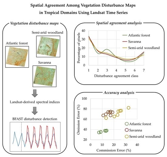
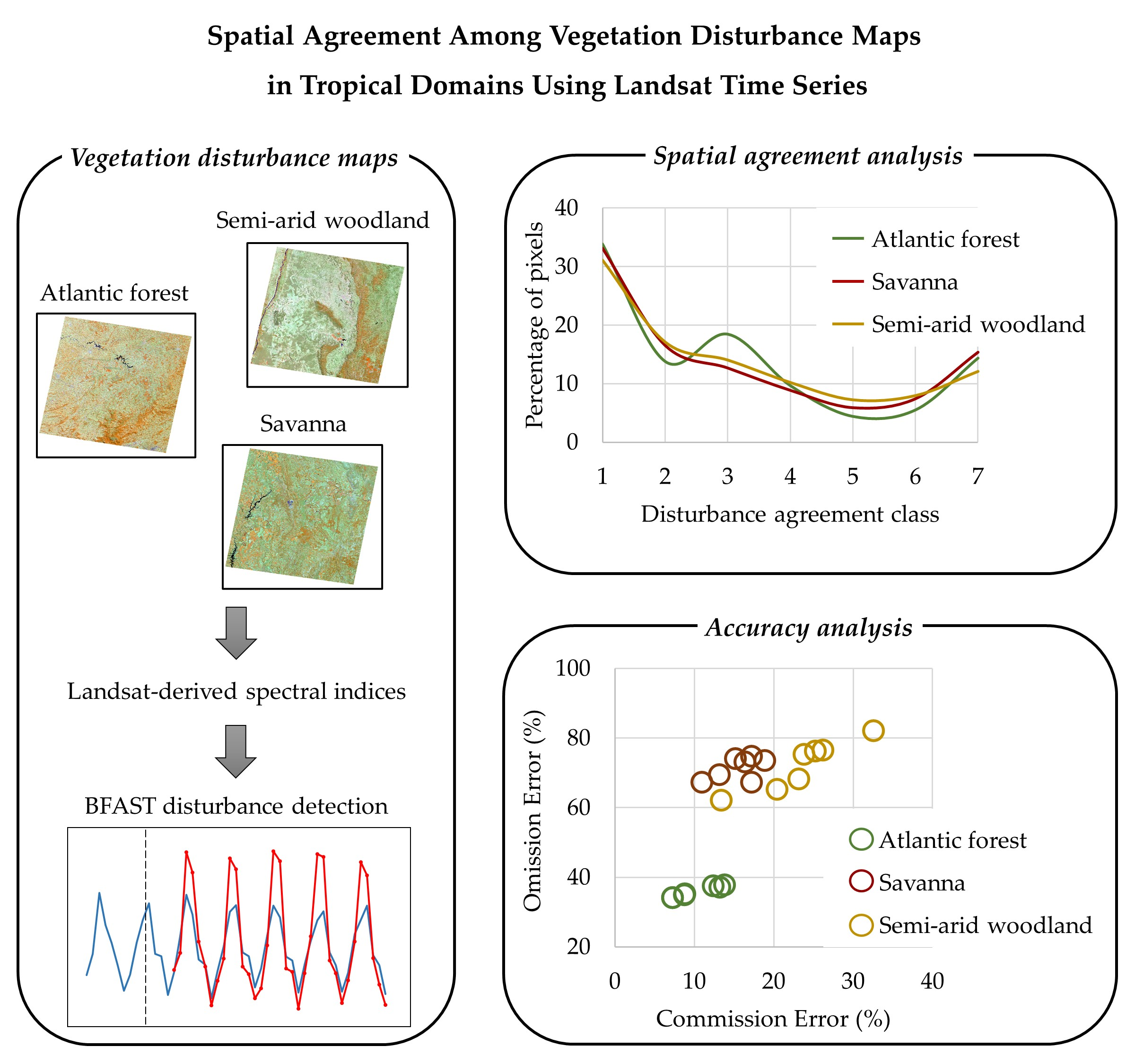
Spatial Agreement among Vegetation Disturbance Maps in Tropical Domains Using Landsat Time Series

by
Inacio T. Bueno
1,
Greg J. McDermid
2,
Eduarda M. O. Silveira
3,*,
Jennifer N. Hird
2,
Breno I. Domingos
1 and
Fausto W. Acerbi Júnior
1
1
Department of Forest Science, Federal University of Lavras, Lavras 37200-000, Brazil
2
Department of Geography, University of Calgary, Calgary, AB T2N 1N4, Canada
3
SILVIS Lab, Department of Forest and Wildlife Ecology, University of Wisconsin-Madison, Madison, WI 53706, USA
*
Author to whom correspondence should be addressed.
Remote Sens. 2020, 12(18), 2948; https://doi.org/10.3390/rs12182948
Submission received: 31 July 2020 / Revised: 31 August 2020 / Accepted: 9 September 2020 / Published: 11 September 2020
(This article belongs to the Special Issue Feature Paper Special Issue on Forest Remote Sensing)

Abstract

:
Detecting disturbances in native vegetation is a crucial component of many environmental management strategies, and remote sensing-based methods are the most efficient way to collect multi-temporal disturbance data over large areas. Given that there is a large range of datasets for monitoring, analyzing, and detecting disturbances, many methods have been well-studied and successfully implemented. However, factors such as the vegetation type, input data, and change detection method can significantly alter the outcomes of a disturbance-detection study. We evaluated the spatial agreement of disturbance maps provided by the Breaks For Additive Season and Trend (BFAST) algorithm, evaluating seven spectral indices in three distinct vegetation domains in Brazil: Atlantic forest, savanna, and semi-arid woodland, by assessing levels of agreement between the outputs. We computed individual map accuracies based on a reference dataset, then ranked their performance, while also observing their relationships with specific vegetation domains. Our results indicated a low rate of spatial agreement among index-based disturbance maps, which itself was minimally influenced by vegetation domain. Wetness indices produced greater detection accuracies in comparison to greenness-related indices free of saturation. The normalized difference moisture index performed best in the Atlantic forest domains, yet performed poorest in semi-arid woodland, reflecting its specific sensitivity to vegetation and its water content. The normalized difference vegetation index led to high disturbance detection accuracies in the savanna and semi-arid woodland domains. This study offered novel insight into vegetation disturbance maps, their relationship to different ecosystem types, and corresponding accuracies. Distinct input data can produce non-spatially correlated disturbance maps and reflect site-specific sensitivity. Future research should explore algorithm limitations presented in this study, as well as the expansion to other techniques and vegetation domains across the globe.

Graphical Abstract

1. Introduction

Anthropogenic disturbances in tropical environments (i.e., selective logging and wildfires) are considered one of the major drivers of biodiversity loss [1] and the second largest source of anthropogenic greenhouse gas emissions [2]. In the 1990–2010 period, global net losses of tropical forests averaged 6 million hectares per year (approximately 0.38% annually) [3]. Such disturbance rates have received worldwide attention as tropical vegetation domains play such a key role in global systems. Overall, they store 200–300 Pg. C (1015 grams of carbon) [4], account for about 60% of the world’s terrestrial photosynthesis [5], provide habitats for more than half of the known species worldwide [6], and are a major regulator of global climate [7].
Mapping disturbances in tropical domains plays a pivotal role in many environmental management strategies, and remote sensing data are the only feasible way to detect and monitor these changes over large areas. However, this is not a trivial task, as change detection is subject to a variety of noise factors including natural forest phenology, cloud cover, atmospheric scattering, and geometric errors [8]. As a result, we require an understanding of the sensitivity and generalizability of change-detection methods across a variety of different vegetation types [9].
The opening of the Landsat archive in 2008 boosted the application of vegetation disturbance detection from satellites. Free global mid-resolution (30 m) remote sensing imagery has enabled more accurate area estimation analysis, characterization of disturbance types, and monitoring post-disturbance conditions [10]. In addition, these new capabilities have been leveraged through the development of new time-series techniques for detecting and tracking disturbances [11]. For example, the Breaks For Additive Season and Trend (BFAST) recently emerged as a reliable automated algorithm for detecting vegetation disturbances across the tropics [12,13,14,15]. BFAST was originally developed for detecting vegetation disturbances from a 16-day Moderate Resolution Imaging Spectroradiometer (MODIS) time series. It computes long-term trends and abrupt disturbances in a dense time series of a spectral index, then produces sub-annual information on disturbances and trends [16]. Later, BFAST Monitor emerged as a near-real time means of identifying disturbances from a stable history period [17].
Recent research has demonstrated the utility of BFAST algorithms and Landsat time series using different spectral indices over a variety of vegetation domains. For example, using Landsat time series and the normalized difference vegetation index (NDVI), BFAST tracked small-scale disturbances in an Afromontane forest [14], and identified annual land cover disturbances and their effect on vegetation greenness in a coastal region [18]. The algorithm was also useful for detecting burned areas in savanna regions, outperforming coarse-resolution burned area products [19]. Moisture-related spectral indices, such as the normalized difference moisture index (NDMI), were also assessed for detecting and attributing causes of disturbances in the Colombian Andes [20], and to identify forest degradation in mixed savanna and dry forest areas [12]. Positive trends in vegetation were evaluated by quantifying vegetation regrowth using the soil-adjusted total vegetation index (SATVI) of abandoned well pads in semi-arid lands [21].
Different spectral indices can return disparate accuracies when mapping disturbances in tropical forests using BFAST. In tropical dry forests, moisture-related indices achieved better spatial accuracies when compared to greenness-related indices [22]. Similar results were found in evergreen forests over the globe, although the canopy-related normalized difference fraction index (NDFI) outperformed moisture-related indices in this instance [13]. Another important element in disturbance detection studies is locational or regional variability, which can influence forest disturbance patterns. Disturbance detection methods over large areas usually opt for generalized vegetation types. A common strategy is to apply a predefined threshold for identifying forested areas and then detecting disturbed pixels when there are significant deviations from the threshold [3,23]. However, disturbance dynamics can differ across forest types, leading to misclassifications in large-scale analysis [24]. Using BFAST, Schultz et al. (2016) [8] observed different levels of edge effects in different sites while detecting forest disturbances. This led the authors to suggest that local forest disturbance patterns must be understood and algorithms must be tuned to account for regional conditions. Furthermore, Grogan et al. (2016) [9], while observing their error distribution over forest types, found a site-specific sensitivity to error imbalances when using a generalized forest model, i.e., they noted disturbance underestimation in evergreen forests and overestimation in dry forests.
Research into Landsat spectral indices is comprehensive and the BFAST algorithms have received attention in tropical forests. However, no study has examined the algorithm’s performance across distinct vegetation domains while also investigating similarities between vegetation disturbance maps derived from different spectral indices. In addition, most recent disturbance detection studies frequently relate to forested areas, while non-forested areas, such as scrublands in savannas or open grasslands in semi-arid lands, are still not yet fully understood.
In this paper, we compare the suitability of several spectral indices for mapping disturbances in different tropical vegetation domains using the BFAST Monitor algorithm. This study addressed the following questions: (1) How do vegetation disturbance maps derived from Landsat-based spectral indices spatially agree? (2) How accurate are these vegetation disturbance maps when compared to a reference dataset? (3) How does the vegetation domain influence these agreements? Thus, our objectives were: (1) To evaluate the spatial agreement between disturbance maps produced using seven spectral indices derived from Landsat Thematic Mapper/Operational Land Imager (TM/OLI) and input into BFAST Monitor, and the influence of vegetation domain on this agreement; and (2) to evaluate the accuracies of these index-derived disturbance maps and their relationship with vegetation domain. To accomplish these objectives, we used a dense Landsat time series from 2003 to 2017 and calculated seven distinct spectral indices to detect disturbed pixels through the BFAST Monitor algorithm. We evaluated the disturbance maps’ accuracies and spatial similarity in three distinct vegetation domains in southeast Brazil: Atlantic forest, savanna, and semi-arid woodland.

2. Materials and Methods
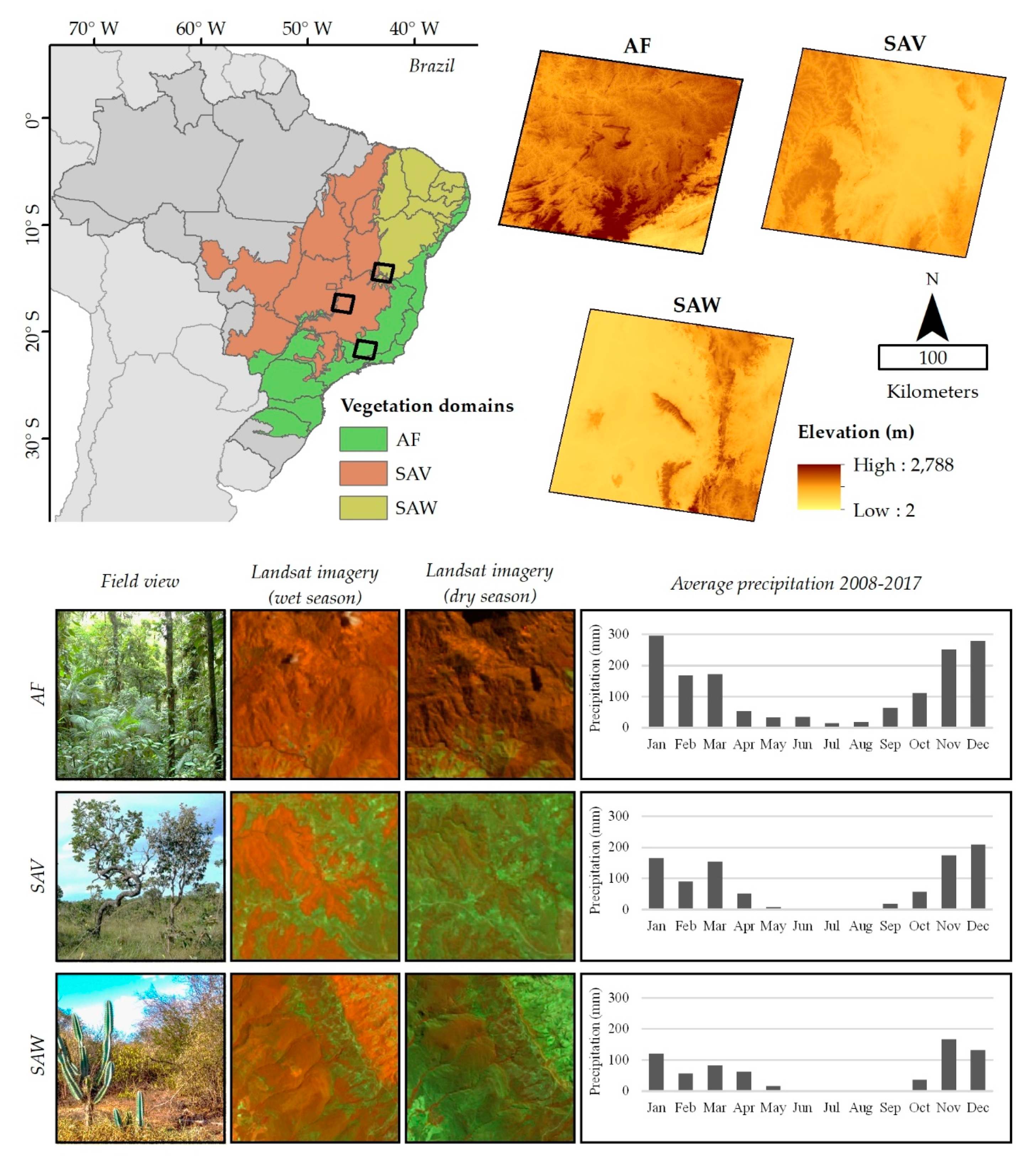
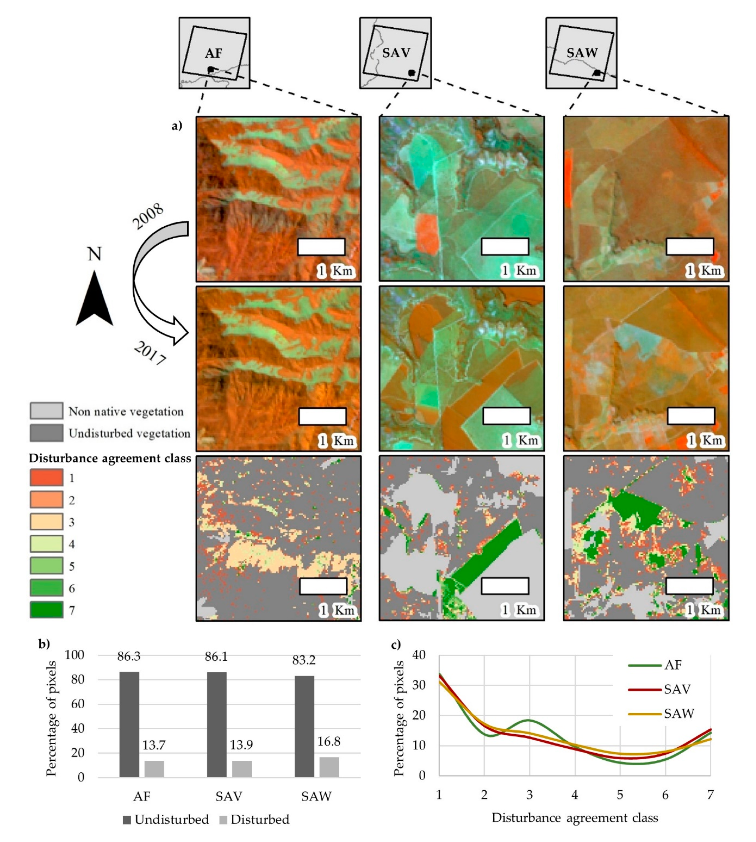
2.1. Study Sites

The study area comprises three Worldwide Reference System grid (WRS-2) scenes dispersed across the Minas Gerais state of southeastern Brazil (Figure 1). These regions represent three distinct Brazilian vegetation domains: Atlantic forest (Path/Row: 218/75), savanna (Path/Row: 220/72), and semi-arid woodland (Path/Row: 218/70).
The Atlantic forest is composed of different types of vegetation, mostly including rainforests, semi-deciduous forests, as well as high-altitude grasslands. This vegetation domain has outstanding levels of species endemism, making the Atlantic forest a biodiversity hotspot [25]. In the past, it was subjected to substantial disturbance activity and was reduced to approximately 14% of its original vegetation [26], becoming one of most vulnerable hotspots to global change [27]. The greatest extent of the Atlantic forest scene is located in the south of the Minas Gerais state, extending over the states of São Paulo and Rio de Janeiro. The region is represented by a mix of plains in the northwest, and the Serra da Mantiqueira mountain complex in the southeast of the scene. This region receives around 2000 mm annual rainfall with lower values into the continent and higher values found at montane areas. Most of the area does not show a climatological water deficit, leading to a low seasonal signal [28].
In Brazil, the savanna vegetation domain is represented by the Cerrado biome, which has a unique vertically structured mosaic of plant formations among the savannas in the world [29]. It ranges from forest formations with dense canopy cover to grasslands with sparse and short twisted trees, also being considered a biodiversity hotspot [25]. The savanna scene is located in western Minas Gerais crossing to Goiás state, where approximately 90% of the rains are concentrated from October to April with annual precipitation ranging from 1200 to 1800 mm. The dry season is quite distinct with monthly precipitation reaching zero millimeters, inducing a wide range of adaptive phenological strategies in vegetation formations in order to overcome water scarcity. The Brazilian savanna has been under increasing anthropic pressure due to policy-driven land conversion processes, as indicated by ~266,000 km2 of gross forest loss in the past twenty years [30].
Semi-arid woodland, also known as the Caatinga biome, is an ecosystem occupied by a mixture of deciduous forests and herbaceous understory. The scene occupies a northeastern portion of Minas Gerais being mostly concentrated in Bahia state, with an extensive area of the Espinhaço mountain range. It receives less than 750 millimeters per year of extremely irregular rainfall, where more than 75% of the total annual rainfall can occur within three months. In addition, annual variations in semi-arid woodland are large where droughts can last for a couple of years. As the Brazilian savanna, these dry forests have been either converted from their native vegetation or modified in a major way, represented by ~90,000 km2 of forest loss with an increase from 0.19% yr−1 to 0.44% yr−1 in the past decades [30].

2.2. Pre-Processing

As our study evaluates disturbances based on a time series modeling algorithm, a non-native vegetation mask is important to limit the procedure to pixels that are established as vegetation at the beginning of the study period. This avoided unnecessary computation time and further uncertainties. For this reason, we used the land use/land cover map of the Brazil’s Rural Environmental Registry (CAR, Cadastro Ambiental Rural in Portuguese) as a vegetation mask. The land use/land cover map used 5 m Rapideye and 30 m Landsat TM imagery to produce a valuable high-resolution large-scale product. This is used as input for land-use, environmental, economic, and territorial policies. CAR’s vegetation class comprises forested areas as well as non-forest native vegetation, i.e. lowland and montane grasslands, shrub lands, scrublands, and wetlands. We additionally masked temporary water bodies that were not accounted for by CAR’s layer using the Global Surface Water information [31], which contains Landsat-based annual maps of the location and temporal distribution of surface water from 1984 to 2018. Temporary surface water is commonly located in the savanna and semi-arid woodland domains represented by veredas and wet grasslands, respectively [32]. They are composed of temporary ponds or streams where water content may range from water-logged soil to water bodies several meters deep. This natural decrease and increase in water levels based on a dry period of varying duration can be a source of noise in vegetation disturbance analysis.

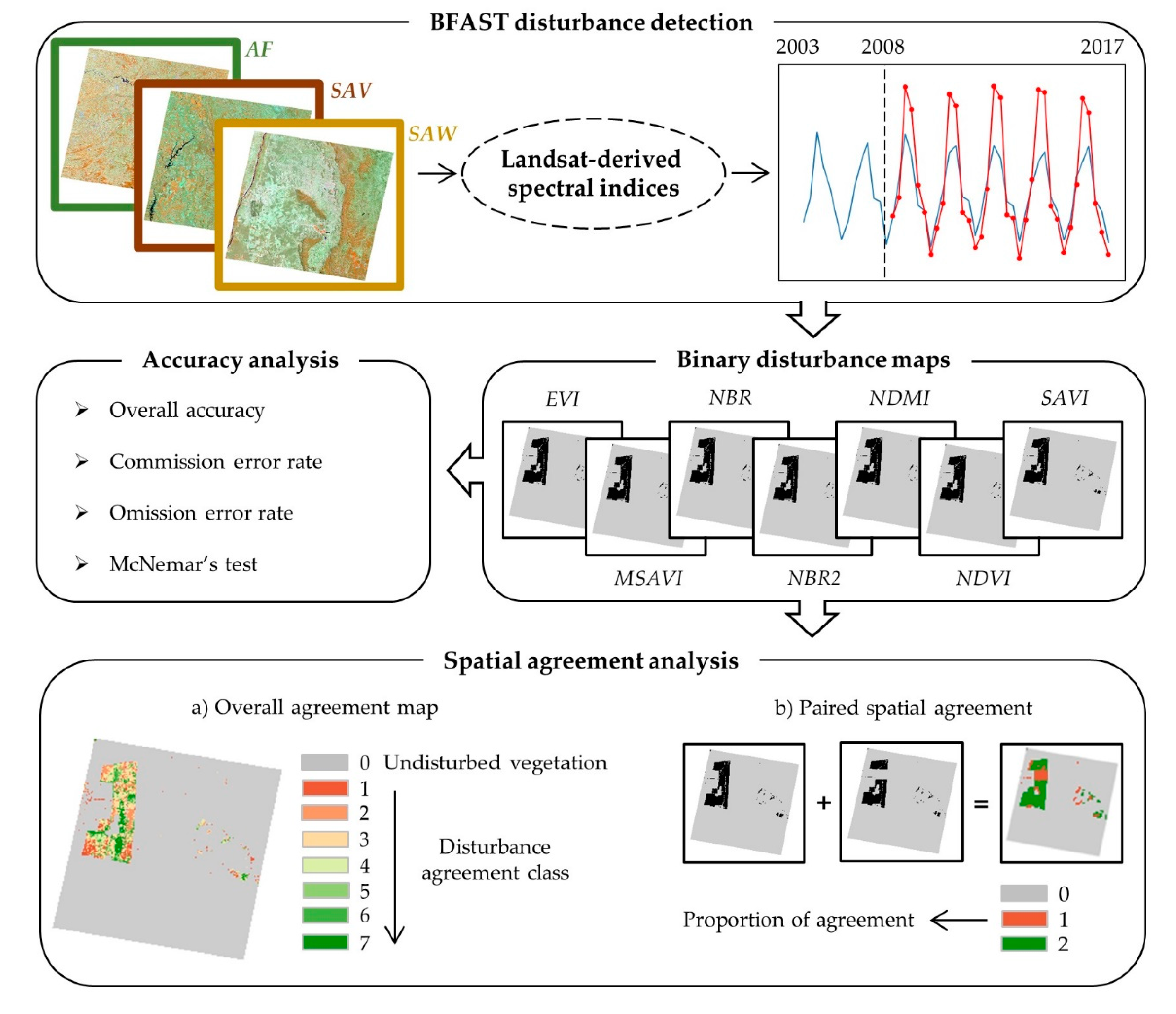
2.3. Landsat-Derived Spectral Indices

We acquired Landsat TM/OLI-derived spectral index products provided by the U.S. Geological Survey’s Earth Resources Observation and Science Center (USGS EROS) [33] from 2003 to 2017 across the three WRS-2 tiles covering the study region. TM and OLI products were converted to surface reflectance using the Landsat Ecosystem Disturbance Adaptive Process (LEDAPS) [34] and Land Surface Reflectance Code (LaSRC) [35], respectively. We selected all images available with less than 50% of cloud cover using the Function of Mask (Fmask) algorithm [36] to generate cloud-free observations.
A set of seven commonly used indices were downloaded from the USGS EROS website, which saved us from performing data preprocessing steps such as geometric and radiometric calibration, and band math calculations. These indices can be grouped into two broad categories based on their calculations using similar spectral wavelengths, and their resultant response to land surface vegetation. The first group employs a combination of red (TM/OLI (0.630–0.690 µm)) and NIR (TM (0.760–0.900 µm), OLI (0.845–0.885 µm)), and respond to actively photosynthesizing biomass. We label these ‘greenness indices.’ They include and are built around the NDVI, the most frequently used index in remote sensing science, that was selected due to its use to quantify vegetation greenness [37]. It is calculated as a normalized ratio between Red and NIR reflectance values (Equation (1)). Higher NDVI values suggest higher amounts of photosynthetic active biomass. As the most popular index, NDVI time series have been used in many forest disturbance detection and monitoring efforts [38,39].
N D V I = N I R R e d N I R + R e d
We include three more greenness indices in this group, all of which are variations of the NDVI and which are designed to reduce saturation issues identified with this index—the enhanced vegetation index (EVI), the soil-adjusted vegetation index (SAVI), and the modified soil-adjusted vegetation index (MSAVI). The EVI, developed by Huete et al. (1999) [40], was selected due its usefulness in regions with dense vegetation as it does not saturate as quickly as other vegetation indices. It incorporates the blue band (TM/OLI (0.450–0.520 µm)), which is atmosphere-sensitive and used to correct aerosol influences in the red band, canopy background adjustment L = 1.0, adjustable coefficients of atmospheric resistance C1 = 6 and C2 = 7.5, and the sensor’s gain factor G = 2.5 (Equation (2)). As an improvement to NDVI regarding saturation issues in highly dense vegetation, EVI also has frequent use in tropical forest disturbance detection [41].
E V I = G × ( N I R R e d N I R + C 1 × R e d C 2 × B l u e + L )
In contrast to EVI, SAVI corrects NDVI by reducing the influence of soil brightness in areas with sparse vegetation [42]. It has a soil brightness correction factor L = 0.5 (Equation (3)), which can be sensitive to deforestation with incomplete forest canopy cover or located at the edge of forest remnants, which is related to forest degradation studies [12].
S A V I = ( 1 + L ) × ( N I R R e d N I R + R e d + L )
Our final greenness index, the MSAVI, modifies SAVI by replacing the constant soil adjustment factor L with a self-adjusting function (Equation (4)) [43]. In this version of MSAVI, the L factor is self-adjusted to the best vegetation density factor, reducing the soil background effects. The MSAVI is shown to increase the dynamic range of the vegetation signal while further minimizing the soil background influences, resulting in greater vegetation sensitivity as defined by a vegetation signal-to-soil noise ratio, showing usefulness for forest degradation studies [44].
M S A V I = 2 × N I R + 1 ( 2 × N I R + 1 ) 2 8 × ( N I R R e d ) 2
In addition to these four greenness indices, we include in our analysis three ‘wetness indices.’ These employ a combination of NIR and shortwave infrared (SWIR) reflectance in their formulae. The latter has shown lower reflectance in vegetation areas compared to other spectral regions due to absorption caused by water and the biochemical content of vegetation. However, they are frequently used in forest fire mapping [45] and forest recovery [46], and due to water-related responses, these indices have also been used in forest disturbances related to anthropic practices [22,47]. The wetness indices included in our analyses are: The normalized burn ratio (NBR), a second version of the NBR (NBR2), and the NDMI. The first two were originally designed for estimating post-wildfire burned area, and burn severity, while the latter is commonly used to track vegetation water content, water stress, and plant biomass changes more closely [48].
The NBR is calculated as a normalized ratio between NIR and the second Landsat SWIR band (SWIR2, TM (2.080–2.350 µm), OLI (2.100–2.300 µm)) reflectance (Equation (5)) [49].
N B R = N I R S W I R 2 N I R + S W I R 2
The second version of normalized burn ratio (NBR2) modifies NBR by replacing the NIR band with the first Landsat SWIR band (SWIR1, TM (1.550–1.750 µm), OLI (1.560–1.660 µm)) (Equation (6)) in order to highlight water sensitivity in vegetation [50]. By using both shortwave infrared channels, this index is very sensitive to leaf moisture and is suitable for deforestation mapping [47].
N B R 2 = S W I R 1 S W I R 2 S W I R 1 + S W I R 2
Finally, the NDMI adjusts the normalized difference formula by replacing the SWIR2 band used in Equation (5) with SWIR1 (Equation (7)). The NDMI has shown good accuracies in forest degradation [12], as well disturbances associated with forest type and harvest intensity [51].
N D M I = N I R S W I R 1 N I R + S W I R 1

2.4. Vegetation Disturbance Maps

In this study, we defined ‘disturbance’ as negative changes to the native vegetation induced by human activity that completely alters the land cover. The main process for this is the conversion of native vegetation to pastures or bare soil by logging practices. To detect these disturbances in native vegetation, we used the R package ‘bfastSpatial’ [17]. BFAST Spatial applies BFAST Monitor over each stack of Landsat indices, where each pixel is represented by a time series. The method of detection is based on fitting a seasonal model on a period defined as having a stable land cover history and then checking the stability of this model during the change analysis period.
We assigned the stable history period to the years 2003 to 2007 and tuned BFAST Monitor to fit a first-order harmonic model in order to describe the native vegetation trajectories under seasonal changes. A first-order harmonic model helps to model the irregular distribution of Landsat observations that can result in model over-fitting [14]. Subsequentially, the monitoring period was assigned to the years 2008 to 2017 where the algorithm detects whether a new observation deviates from the stable history model. By computing a moving sum of the residuals based on an ordinary least squares model, a breakpoint is flagged when the moving sum deviates from zero beyond a 95% significance threshold.
We extracted the magnitude-of-change from model breakpoints, where negative magnitude values are associated with vegetation loss (i.e., deforestation, wildfires, forest degradation) and positive values are with vegetation cover gain (i.e., forest regeneration). However, model breakpoints may be associated with near-zero disturbance magnitudes that are not related to anthropic events; thus, a secondary classification arises as an important step to better distinguish anthropogenic disturbances from stable areas affected by seasonal variations [14]. For this reason, we defined a threshold of disturbance to obtain a binary map (disturbed, undisturbed).
We then applied a threshold-based method to determine the binary changes by setting a fixed percentile of 10% (5% on each tail) of the data distribution. Particularly, a pixel was assigned as disturbed (value = 1) when its magnitude-of-change value was less than 5% of negative values or greater than 5% of positive values. Otherwise, it was assigned as undisturbed (value = 0). Positive change magnitude values (vegetation cover gain) were also classified as disturbance because a vegetation pixel with low reflectance values, i.e., scrublands, may be abruptly converted to high-reflectance land use, i.e., agriculture lands, which can result in a positive value of change along the time series. The selection of a suitable threshold value to identify change has been reported as a difficult task and is arbitrary as it is directly related to the exclusion and inclusion of change areas [52]. However, this procedure guarantees the inclusion of an equal number of pixels of the index gain and loss, making it suitable to compare how change maps are similar through a unique change algorithm.
It is worth recalling that our purpose here was not to produce the most accurate disturbance maps, but rather to compare effects of spectral indices and vegetation domain on different disturbance maps produced with consistent (and reasonable) workflows.

2.5. Spatial Agreement and Accuracy Analysis

Our procedure consisted of a spatial analysis of disturbed pixels adapted from Cohen et al. (2017) [53] and performed on individual study scenes. We then compared disturbance maps with one another (spatial agreement analysis) to a reference dataset (see Section 2.5.3 Accuracy analysis) as illustrated in Figure 2. The first component—spatial agreement—was divided into two parts: (a) Overall agreement among the seven disturbance maps, and (b) paired agreement between maps.

2.5.1. Overall Spatial Agreement

The overall-agreement analysis consisted of summing the seven binary disturbance maps, producing an overall agreement map by vegetation domain. For each pixel, the number of maps labels that pixel as disturbance, producing an overall agreement map with eight numerical classes. These classes varied from one (meaning that only one particular spectral index detected a disturbance in a particular pixel) to seven (meaning a total agreement among disturbance maps for a disturbed pixel). The total agreement for undisturbed pixels was assigned as undisturbed vegetation. The number of pixels per class was extracted and plotted across the vegetation domains. In addition, we isolated classes ‘one’ and ‘two’ from the overall agreement map (hereafter labeled as ‘class1‘ and ‘class2’), then analyzed these by ranking what indices most contributed for these low agreement counts. Class1 and class2 describe the lowest amounts of spatial agreement observed among the spectral indices in that they reflect locations where disturbance is detected by only one or two spectral indices, respectively.
We analyzed these classes to better understand which indices contributed most to disturbance detection disagreements. Furthermore, we compared the influence of vegetation domain in map agreement. A one-way analysis of variance (ANOVA) was used to test whether agreement classes were significantly different across vegetation domains. If the difference was significant, the test indicated that vegetation domains affect the spatial agreement among vegetation disturbance maps.

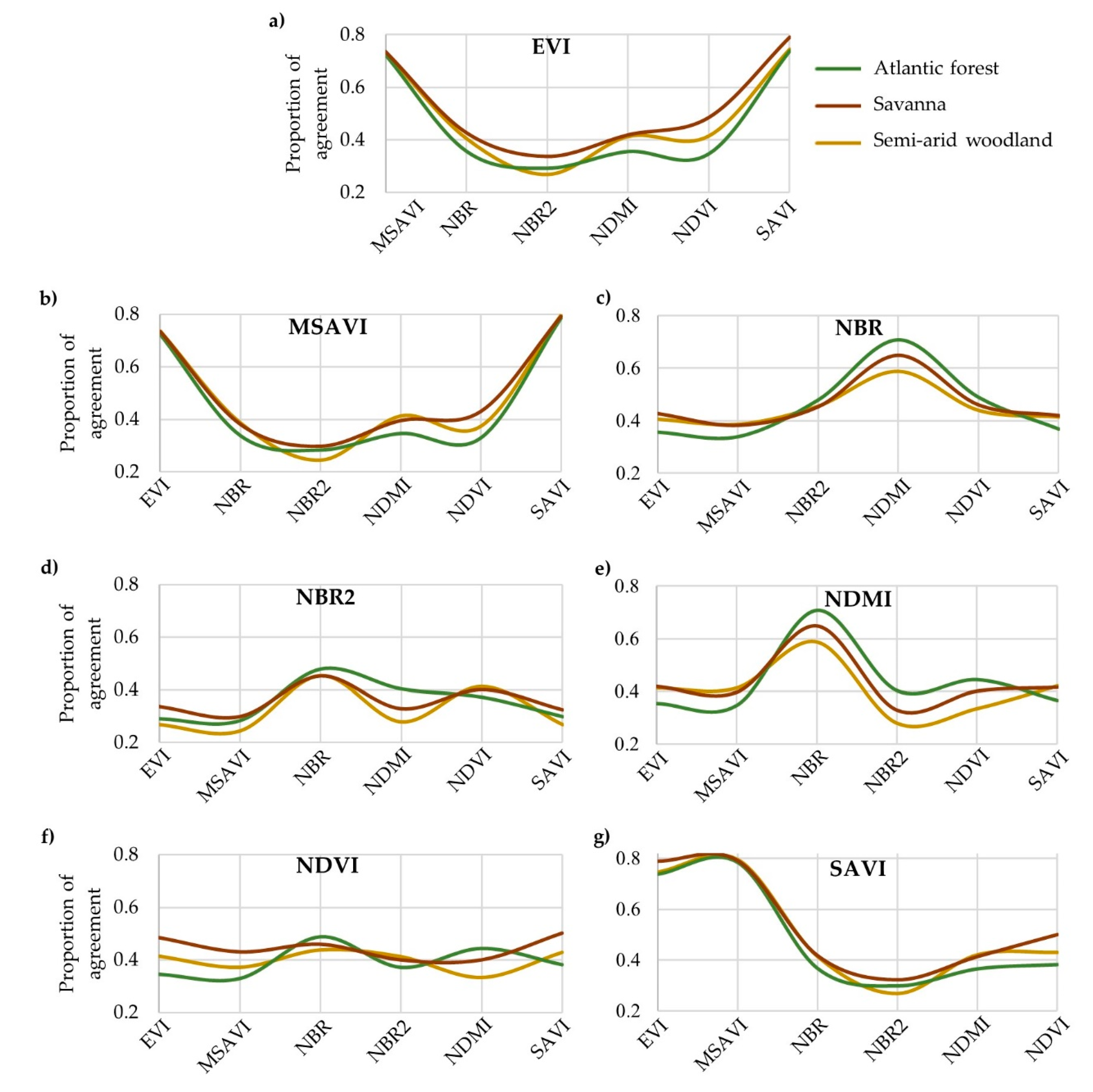
2.5.2. Paired Agreement

To evaluate the spatial agreement of an individual disturbance map with those produced using the other six spectral indices and BFAST Monitor, we assessed paired agreement between individual maps. This paired agreement evaluation consisted of analyzing the similarity between two maps by vegetation domain. Similar to the overall agreement, here, we summed pairs of binary disturbance maps, which returned pixel classes of 0 (agreement to undisturbed class), 1 (disagreement), or 2 (agreement to disturbance class).
We calculated the proportion of agreement of a map i with a map j by summing the agreement of disturbed pixels Nij and dividing by the number of disturbed pixels in both maps Ni and Nj, minus Nij (Equation (8)). Proportions varied from 0 (total disagreement) to 1 (total agreement). Afterward, we plotted the paired agreement across the vegetation domains in order to produce a comprehensive visual interpretation.
A g r e e m e n t i , j = N i j N i + N j N i j

2.5.3. Accuracy Analysis

For the accuracy analysis, we compared each disturbance map with a reference data set to quantify its accuracy. Reference data were compiled by creating fixed-area plots and then delineating disturbance polygons within the plot by visual interpretation using Landsat images. High-resolution imagery from Google Earth were also used, where available, as auxiliary information to infer land cover changes in ambiguous areas, i.e., non-native vegetation areas included in the vegetation map mask. Square plots of 120 km2 were placed across each vegetation domain study area using a systematic point grid of 45 km by 45 km over the scenes. This sampling design represented 5% of each study area and was sufficiently large to contain a suitable number of deforestation observations [54].
In order to balance the number of observations per class, we randomly selected 25 pixels per class (disturbed and undisturbed) in each area plot. A total of 1950 pixels (25 × 2 classes × 13 area plots × 3 scenes) were used to analyze the change maps. We calculated accuracy measures for each map by summing the correctly detected observations and dividing by (a) the total number of observations (overall accuracy), (b) the proportion of the total number of observations labeled as disturbance in the reference but not labeled by a given map (omission rate), and (c) the proportion of the total number of observations labeled as disturbance by a map set but not labeled by the reference (commission rate).
We used ANOVAs to test whether there were significant differences in accuracy statistics across vegetation domains. We performed three separate tests, one for each accuracy statistic: Overall accuracy, producer’s accuracy, and user’s accuracy. Each test had three groups (vegetation domains) of seven samples (indices). The null hypothesis was that the relevant test statistics all came from the same population.
We also performed McNemar’s tests to determine if there were statistically significant differences between the various pairwise map accuracies. McNemar’s test is a non-parametric test based on chi-square (χ2) statistics with 1 degree of freedom, which can be computed from two confusion matrices, and is suitable for assessing distinct mapping performances [55]. McNemar’s test was applied using the R package ‘stats’ at a 95% confidence level and included a continuity correction to account for having a discrete statistic in a continuous distribution.

3. Results

3.1. Spatial Agreement Analysis

Overall disturbance map agreement insets are displayed in Figure 3a. These show the visual agreement between the different index-based maps with regard to the disturbed vegetation class. Considering each vegetation domain, the percentage of disturbed pixels in the overall disturbance map, wherein disturbed pixels are those where disturbance was detected by one or more spectral indices, was 13.7% in the Atlantic forest, 13.9% in the savanna, and 16.8% in the semi-arid woodland (Figure 3b).
In general, the agreement analyses returned a similar trend in disturbance agreement classes across the three vegetation domains, indicating that the latter did not influence patterns of spectral-index performance (Figure 3c). These results are reinforced by the ANOVA that revealed no statistically significant differences across vegetation domains with F(2, 18) = 0.239 (p-value = 0.789). Mean (standard deviation) F-statistics for Atlantic forest, savanna, and semi-arid woodland were 1.95 (1.36), 1.98 (1.28), and 2.39 (1.37), respectively.
For savanna and semi-arid woodland, the highest percentages of disturbed pixels were represented by class1 (33.1% and 31.1%, respectively) and class2 (16.6% and 17.2%, respectively). For Atlantic forest, the highest percentage of disturbed pixels was represented by class1 and class3, with 33.8% and 18.4%, respectively (Figure 3c). Table 1 provides the proportion that each spectral index disturbance map contributes to the classes class1 and class2 of the overall agreement map. NBR2 contributed the most to class1 agreement (Atlantic forest = 39.7%, savanna = 43.1%, and semi-arid woodland = 39.5%) followed by NDVI and NDMI. Class2 was very balanced across the spectral indices in the Atlantic forest domain; however, in the savanna and semi-arid woodland domains, moisture indices, represented by NBR, NBR2, NDMI, and NDVI, were responsible for a high proportion of this class.
Exploring the spatial relationships between individual spectral indices, there was an observable pattern in agreement across vegetation domains (Figure 4). Proportions of paired agreement greater than 0.70 (see Equation (8)) were expressed by EVI, MSAVI, SAVI, and their paired combinations, presenting the highest values of spatial agreement for all vegetation types. In addition, NBR and NDMI also presented high values of similarity among the vegetation domains (Atlantic forest = 0.71, savanna = 0.65, and semi-arid woodland = 0.59).
On the other hand, low proportions of agreement were produced by NBR2 and its combinations with EVI, MSAVI, and SAVI (<0.30) for the three vegetation domains as well. Low values of spatial agreement between the NBR2 index and other indices corroborate our earlier results in Table 1 with regard to the large contribution of this index to class1, at about 40%. Although NBR2 presented very low similarity with most of the indices, exceptions were noticed with NBR (Atlantic forest = 0.48, savanna = 0.45, and semi-arid woodland = 0.46) and NDVI (Atlantic forest = 0.37, savanna = 0.40, and semi-arid woodland = 0.41).

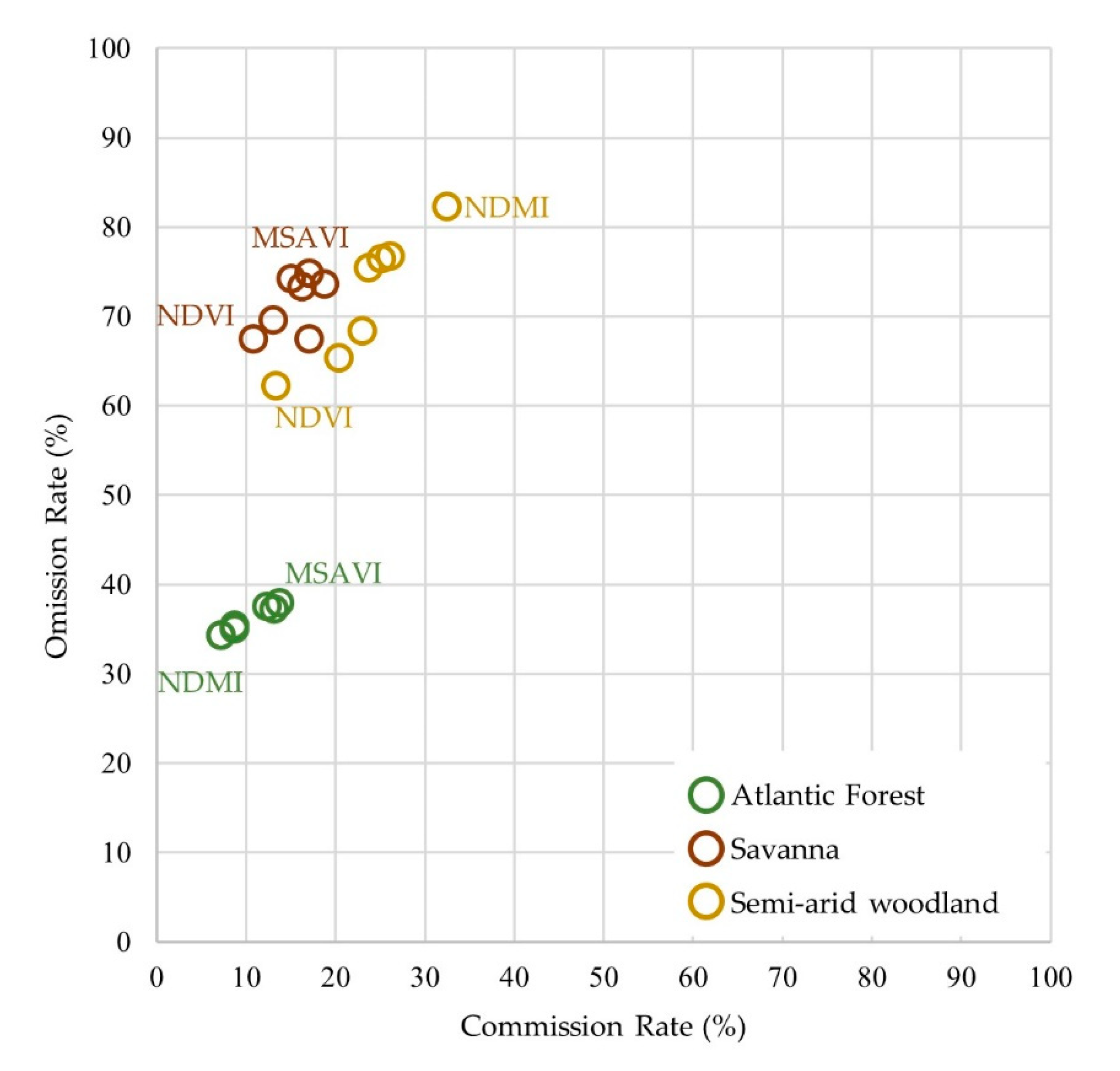
3.2. Accuracy Analysis and Index Performance

Map accuracies are presented in Table 2. Overall accuracies varied across vegetation domains and varied slightly among indices. Among the study areas, NBR and NDMI indices in the Atlantic forest domain presented the highest overall accuracies of 82.1%, while the lowest result was registered by MSAVI map (78.2%). NDMI presented the poorest results for semi-arid woodland at 54.6% overall accuracy. NDVI produced the highest overall accuracy for both semi-arid woodland (66.0%) and savanna (59.6%). Although savanna accuracies fell between the other two domains, it demonstrated a lower overall accuracy average when compared to semi-arid woodland, 56.6% versus 59.8%, respectively.
Commission error, inversely related to the user’s accuracy, was variable among the vegetation types (Figure 5). Atlantic forest commission error rates followed overall accuracy trends across spectral indices, presenting low commission error rates by NDMI and NBR (7.3%), and the highest error rate by MSAVI (13.8%). In the semi-arid woodland vegetation domain, NDMI presented again higher error rates compared to its performance in the Atlantic forest, with the highest commission error for the former vegetation domain at 32.6%. Semi-arid woodland and savanna showed NDVI to produce the lowest commission errors at 10.9% and 13.4%, respectively.
Omission error, inversely related to the producer’s accuracy, presented considerable variability throughout the vegetation domains. A spectral index performance hierarchy similar to what was observed in overall accuracies and commission errors was observed in the Atlantic forest, with NDMI and NBR producing the lowest omission error rates (34.2%), and MSAVI producing a 37.9% error rate. Results for the savanna vegetation domain followed a similar pattern.
Finally, semi-arid woodland possessed the highest omission rate among all disturbance maps, represented by 82.2% in the NDMI disturbance map. As in the commission analysis, NDVI produced the lowest errors of omission in semi-arid woodland and savanna, at 62.2% and 67.4%, respectively. Our ANOVA revealed statistically significant differences for the three measures of accuracy across vegetation domains with F(2, 18) = 165.3, p-value < 0.0001 for overall accuracy; F(2, 18) = 19.0, p-value < 0.0001 for commission error; and F(2, 18) = 140.2, p-value < 0.0001 for omission error. Mean and standard deviations for vegetation domains are presented in Table 2.
The McNemar’s test showed no statistically significant differences between spectral indices’ disturbance map accuracies in either the Atlantic forest or savanna. However, in the semi-arid woodland, there were significant differences between disturbance accuracies. The NDMI disturbance map, which provided the poorest accuracies in this vegetation domain, was statistically different from NBR, NBR2, and NDVI, the top three performing indices. The NDMI also produced the greatest paired difference in accuracies among all map comparisons (χ2 = 16.62, p-value < 0.0001) when tested against NDVI disturbance map accuracy. NDVI also presented significant differences with other spectral index maps, including EVI, SAVI, and MSAVI (Table 3).

4. Discussion

4.1. Vegetation Disturbance Mapping Using BFAST

An initial objective of this study was to identify how maps derived from Landsat based on spectral indices agree in terms of the vegetation change they detect, and how much the vegetation domain impacts their agreement. Vegetation disturbance maps, provided by one change detection algorithm (BFAST Monitor) and seven different spectral indices (EVI, MSAVI, NBR, NBR2, NDMI, NDVI, and SAVI), indicated a low rate of spatial agreement when compared among themselves. This result is consistent with Cohen et al. (2017) [53], who evaluated forest disturbance derived from seven independent Landsat-based algorithms that presented widely varying disturbance rates. However, our observed rates of agreement were higher than those previously reported by Cohen et al. (2017) [53], which can be expected as we exclude the variability by different classification systems associated with land cover, and explored mostly the spectral variation.
In examining our spatial agreement results in more detail, we observed interesting similarities between spectral indices of similar types (i.e., greenness vs. wetness indices) and their disturbance detection maps across the different environments in our three vegetation domains. For instance, the three greenness indices adjusted for signal saturation (i.e., the EVI, SAVI, and MSAVI) increase the dynamic range of the vegetation signal, which induces a higher sensitivity to topographic illuminations effect and leads to significant changes in the observed spectral characteristics of areas with strong topographic relief. This is observed in the unusual trend in the Atlantic forest domain illustrated by a high frequency of agreement pixels in class3 (three spectral indices disturbance detection through the BFAST Monitor in the overall agreement map). In this case, BFAST change detection, based on these three greenness indices adjusted for saturation, detected high rates of disturbance in the Serra da Mantiqueira region (highlighted by the Atlantic forest inset in Figure 3), which represents roughly one quarter of the forested area in the Atlantic forest vegetation domain.
We also observed the two wetness indices that employ NIR in their formulae, i.e., NBR and NDMI showed spatial agreements that reflected the difference in their use of SWIR1 versus SWIR2, respectively. That is, SWIR 2 shows a lower reflectance than SWIR 1 in native vegetation spectral signatures due to higher levels of absorption by leaf water content, which is a contributing factor in the savanna and semi-arid woodland domains. In addition, the agreement of NDMI with other indices (Figure 4e) was influenced by vegetation domains, indicating lower proportions in semi-arid woodland and higher proportions in Atlantic forest domains, with savanna regions lying in between. This suggests an association between NDMI and levels of moisture-related forest seasonality, leading to changes in NDMI performance over dry-deciduous versus evergreen forest.
In contrast to the greenness and wetness spectral indices discussed above, the NBR2 and NDVI showed the lowest rates of spatial agreement with other indices in this study. The first of these—a wetness index—utilizes only shortwave infrared channels in its formula. In part, the low disturbance map agreement produced by this index is clearly demonstrated by class1 in the overall agreement map (Table 1). In this disturbance agreement class, which indicated pixels labeled by only one vegetation disturbance map, NBR2 accounted for 40% of all pixels in the class. In comparison to the other wetness indices, NBR2 presented a higher agreement with NBR (both indices share the SWIR 2 channel in their formulae) than NDMI (indices sharing SWIR 1 channel) in all three vegetation domains (Figure 4d), providing some support for the conceptual premise that both NBR and NBR2 were developed for burn purposes.
The other low-agreement result produced by the NDVI vegetation disturbance map showed an unusual pattern of agreement among the vegetation domains (Figure 4f). This greenness index can be insensitive to high-density vegetation or soil brightness conditions. This may explain the inverse pattern of performance across vegetation domains to what we observed in wetness index disturbance map agreements—a pattern not observed for the other greenness indices that account for signal saturation. That is, we see from NDVI a low spatial agreement with other indices in the Atlantic forest, followed by better agreement in semi-arid woodland and savanna. In the Atlantic forest, this pattern is related to the lower sensitivity of the NDVI to dense vegetation than that of the other greenness indices, leading to a low rate of misclassification due to topographic illumination effects. In the savanna and semi-arid woodland domains, where high-density vegetation is not a typical feature, higher rates of agreement were observed between the NDVI disturbance maps and those from other indices in the semi-arid woodlands due to the presence of mountainous areas comprised mostly of the Serra do Espinhaço mountain range, versus rates of agreement in the savanna domain.

4.2. Vegetation Sensitivity to Spectral Indices

Our second research question was concerned with how accurate forest disturbance maps are based on real change events. In general, previous studies have mapped vegetation disturbance using BFAST and Landsat time series, reaching satisfactory accuracies. For example, in evergreen forested areas, DeVries et al. (2015) [14] estimated an overall accuracy of 78% with commission and omission rates of 17% in southern Ethiopia. In our study, we found similar results in the Atlantic forest domain, with average overall accuracies at 80.3%, and commission and omission rates of 10.2% and 35.9%, respectively. On the other hand, vegetation domains in this study that are more affected by seasonal variations—savanna and semi-arid woodland—presented poor overall accuracy results ranging from 54.7 to 66.0%. Others studies using BFAST in dry regions reached satisfactory accuracies, such as Schultz et al. (2018) [12] who assessed vegetation degradation in Africa savannas, and found a drop in detection performance as vegetation cover decreased. Likewise, Watts and Laffan (2014) [56] using MODIS EVI assessed vegetation greening changes related to known floods in Australia’s semi-arid regions, finding a BFAST sensitivity to vegetation cover type and seasonal patterns. However, our study faced broad seasonal vegetation domains encompassing mixed forest landscapes and grassland ranges, without a more detailed vegetation classification.
Similar to spatial agreement results, spectral indices can be grouped by their individual accuracy performances. In general, wetness indices and NDVI presented higher accuracies in all vegetation types. These results reflect those of Schultz et al. (2016) [13] and DeVries et al. (2016) [50] who also found particular moisture indices highly correlated with disturbances in tropical forests. SWIR-based indices were also highly related to vegetation change detection in seasonal savannas [47] and herbaceous biomass in semi-arid areas [57]. However, the high accuracies presented by NDVI is somewhat surprising given the fact that studies showed low accuracies related to this index in tropical forests [13,47]. This is a particularly useful result indicating why NDVI is still the most frequently used index in remote sensing, and has been presented in forest disturbances detection and monitoring [38,39].
Another particular occurrence observed in our accuracy analysis was related to the NDMI, which presented a distinct accuracy pattern among vegetation domains. In the Atlantic forest domain, this index had the highest accuracies, as highlighted in Figure 5. In savanna, it was the fourth-best performing among the indices, producing the lowest accuracy among the wetness indices but still higher than that of the greenness indices. However, this index had the lowest accuracies in dry forests, which were statistically different from those of other indices when analyzed by McNemar’s test. These results confirm the relationship between NDMI and vegetation domains observed in our map agreement results, reinforcing a specific sensitivity to vegetation water content, which is more abundant when more vegetation is present.
Greenness-related indices used in this study that adjusted for signal saturation (EVI, MSAVI, and SAVI) were less successful in our accuracy analysis. They were not able to properly isolate the change signal when run through the BFAST Monitor algorithm, generating disturbance misclassifications. Most of their inaccuracies were due to the topographic illumination artifacts, which were also reported by Tan et al. (2013) [58] who found a decrease in the accuracy of disturbance detection practices using Landsat imagery.
Vegetation densities were also a source of error for these greenness indices as high densities can increase the dynamic range of the vegetation signal, which renders it more sensitive to topographic illuminations effects, whereas low vegetation densities can be confused with the corrected soil signals, affecting the disturbance detection accuracy. These results are in keeping with previous observational studies, in which EVI and SAVI also proved to be unsuitable for deforestation detection by [13], or in the case of SAVI, unsatisfactory for assessing forest fire disturbances and recovery [59].

4.3. Considerations and Future Research

Further research on this topic needs to be undertaken before we can clearly understand the relationship between spectral indices using BFAST and their vegetation disturbance detection performances in distinct vegetation types. Some considerations are apparent from this study, such as concerns regarding (1) image preprocessing, (2) algorithm implications, (3) generalization error, and (4) computation timing over large areas.
Image preprocessing is a crucial procedure in disturbance detection studies. The data quality of Landsat products processed at the surface reflectance level by LEDAPS and LaSRC supports time series analysis and data stacking with satisfactory precision (RMSE < 12 m) [11]. In addition, the detection of clouds and cloud shadows is an inevitably required step in time series disturbance detection analysis, particularly in the BFAST Monitor concept that runs on image stacks, not composites. However, Landsat cloud- and cloud shadow-masked products still contribute to misclassifications and may impact disturbance detection analysis as we selected images available with less than 50% of cloud cover detected by the Fmask [36]. These misclassifications can be observed in cloudy regions, such the Serra da Mantiqueira. In addition to preprocessing, another source of uncertainty is related to non-native vegetation mask errors, which also influence the analysis. As is the case for the cloud mask, land cover/land use and surface water maps were not perfect and also include misclassifications. Besides commission- and omission-related class errors, mask boundaries and spectrally mixed pixels were sources of commission rates in this study.
Some sources of error regarding deforestation detection using BFAST on Landsat time series were previously reported by Schultz et al. (2016) [8]. The authors demonstrated radiometric correction strategies for monitoring change in the tropics in relation to differences resulting from data availability, signal-to-noise ratio, atmospheric contamination, and deforestation type. Grogan et al. (2016) [9] reported the use of filtered MODIS time series in order to improve forest change detection, despite BFAST being able to handle unfiltered data. Although we did not analyze the accuracy outputs as they related to image observation frequency, it is was also described as a methodological challenge by Schultz et al. (2016) [13], who demonstrated improved performance in particular spectral indices as a result of increased observation frequencies.
Additional uncertainty arises from the fact that BFAST Monitor was employed across our vegetation domains without substantive calibration for extant conditions within those particular study areas, such as the order of the harmonic model used to fit the stable land cover history, and the h parameter used to determine the potential number of breaks that can be detected by the algorithm. This perhaps points to a need for a more thorough examination of the algorithm performance for each new forest system encountered [53].
In our study, single index performances were related to vegetation domains, where a particular spectral variable produced high accuracies in one domain and lower accuracies in another. For example, NDMI was the most successful index in the Atlantic forest with regard to accuracy while producing the poorest results in the semi-arid woodland. This highlights the fact that large-area monitoring programs covering different ecosystems and land cover types therefore require region-specific spectral variables and individual model calibrations [12], as the highly variable and complex spectral response of different types of forest disturbances across diverse ecosystems clearly increase the odds of generalization errors. These results also support the data fusion approach in change detection applications. This particular method proposes the combination of data inputs (in this case, spectral indices) and their distinctive features in order to increase the global performance. Data fusion methods have already been used by some forest change detection studies, i.e., Healey et al. (2018) [60] mapped forest change detection using an ensemble method of eight Landsat-based algorithms and spatial predictors, reaching higher accuracies with all datasets combined. By fusing multiple index-based disturbance maps derived from LandTrendr [61] and BFAST [13] algorithms, through a random forest scheme, error rates were reduced in comparison to single index outputs. Combining multiple algorithms and spectral indices, Hislop et al. (2019) [62] integrated two algorithms—LandTrendr and a statistical boundary approach—and three spectral indices—NBR, NDVI, and TCW—in order to detect abrupt disturbances in forest environments, which resulted in satisfactory disturbance detection accuracies. Thus, a further study with more focus on data fusion models of different types of forest disturbances across diverse vegetation domains is, therefore, suggested, as feature-level data fusion may produce better results for deforestation disturbance detection than the application of individual spectral indices.
In addition, ancillary data as land cover/land use classifications should be explored in order to mitigate sources of error. Mainly in heterogeneous landscapes, detailed land classes, i.e., classifying woodland from scrublands in savanna regions, are an important approach for avoiding generalization errors and improving BFAST detection accuracies. Another source of uncertainty in this work is related to disturbance types and their magnitudes, as we only assigned disturbances in vegetation as human-induced activities that abruptly remove the native vegetation. Alternative input data are also important as previous studies have reported that canopies can cover sensitive spectral indices such as the NDFI, which demonstrated good performance in tropical forests disturbance detection, and it is calculated using spectral mixture analysis [13]. However, the decision to conduct our study using easily requested spectral index products available on the USGS website avoided data preprocessing steps.
Finally, further challenges in applying BFAST Monitor for Landsat time series analyses relate to processing time when assessing large-scale vegetation disturbance scenarios. Although high-performance and cloud-computing systems are becoming popular, we used parallel processing capabilities on a desktop computer and experienced considerable computational times while processing our data. Advances in high-performance or cloud computing for vegetation disturbance mapping using BFAST Monitor should be explored. For instance, the establishment of cloud platforms such as Google Earth Engine (GEE) provide many advantages for change detection studies, such as direct access to image time series, the straightforward management of time series stacks, and agile computation through parallel processing [63]. These advances might enable the development of large-scale vegetation disturbance maps, and also a user-friendly format to run the BFAST Monitor algorithm.

5. Conclusions

This work contributes to existing knowledge of the performance of vegetation indices from Landsat time series in vegetation disturbance detection by comparing the suitability of spectral indices and their agreement in tropical vegetation domains using BFAST Monitor. We demonstrated that (1) vegetation disturbance maps provided by one change detection algorithm and seven different spectral indices can produce a low rate of spatial agreement when compared, and (2) vegetation domains do not influence this spatial agreement.
With regard to disturbance detection accuracies, wetness indices (NBR, NBR2, and NDMI) outperformed other spectral indices, including greenness-related indices (EVI, MSAVI, and SAVI). NDMI presented the highest accuracy in the Atlantic forest domain while NDVI performed better across savanna and semi-arid woodland domains.
Despite its exploratory nature, this study offered some insight into vegetation disturbance maps and the influence of spectral index choice on the spatial distribution of results, and on detection accuracies. This research has raised many questions in need of further investigation, such as the use of region-specific approaches in order to mitigate the generalization error. Future research should also explore the BFAST Monitor algorithm’s computational limitations presented in this study, as well as its expansion to other techniques and regions across the globe, perhaps with the help of cloud-based processing and analysis platforms.

Author Contributions

Methodology, I.T.B. and B.I.D.; writing—original draft preparation, I.T.B.; writing—review and editing, I.T.B., G.J.M., E.M.O.S., J.N.H., and F.W.A.J.; supervision, G.J.M. and F.W.A.J.; project administration, I.T.B. All authors have read and agreed to the published version of the manuscript.

Funding

This research received no external funding.

Acknowledgments

The authors are grateful to the Coordenação de Aperfeiçoamento de Pessoal de Nível Superior (CAPES) for supporting this work.

Conflicts of Interest

The authors declare no conflict of interest.

References

  1. Barlow, J.; Lennox, G.D.; Ferreira, J.N.; Berenguer, E.; Lees, A.C.; Mac Nally, R.; Thomson, J.R.; Ferraz, S.F.B.; Louzada, J.; Oliveira, V.H.F.; et al. Anthropogenic disturbance in tropical forests can double biodiversity loss from deforestation. Nature 2016, 535, 144–147. [Google Scholar] [CrossRef] [Green Version]
  2. van der Werf, G.R.; Morton, D.C.; DeFries, R.S.; Olivier, J.G.J.; Kasibhatla, P.S.; Jackson, R.B.; Collatz, G.J.; Randerson, J.T. CO2 emissions from forest loss. Nat. Geosci. 2009, 2, 737–738. [Google Scholar] [CrossRef]
  3. Achard, F.; Beuchle, R.; Mayaux, P.; Stibig, H.-J.; Bodart, C.; Brink, A.; Carboni, S.; Desclée, B.; Donnay, F.; Eva, H.D.; et al. Determination of tropical deforestation rates and related carbon losses from 1990 to 2010. Glob. Chang. Biol. 2014, 20, 2540–2554. [Google Scholar] [CrossRef] [PubMed]
  4. Pan, Y.; Birdsey, R.A.; Fang, J.; Houghton, R.; Kauppi, P.E.; Kurz, W.A.; Phillips, O.L.; Shvidenko, A.; Lewis, S.L.; Canadell, J.G.; et al. A large and persistent carbon sink in the world’s forests. Science 2011, 333, 988–993. [Google Scholar] [CrossRef] [PubMed] [Green Version]
  5. Mitchard, E.T.A. The tropical forest carbon cycle and climate change. Nature 2018, 559, 527–534. [Google Scholar] [CrossRef] [PubMed]
  6. Tovo, A.; Suweis, S.; Formentin, M.; Favretti, M.; Volkov, I.; Banavar, J.R.; Azaele, S.; Maritan, A. Upscaling species richness and abundances in tropical forests. Sci. Adv. 2017, 3, e1701438. [Google Scholar] [CrossRef] [PubMed] [Green Version]
  7. Lawrence, D.; Vandecar, K. Effects of tropical deforestation on climate and agriculture. Nat. Clim. Chang. 2015, 5, 27–36. [Google Scholar] [CrossRef]
  8. Schultz, M.; Verbesselt, J.; Avitabile, V.; Souza, C.; Herold, M. Error Sources in Deforestation Detection Using BFAST Monitor on Landsat Time Series Across Three Tropical Sites. IEEE J. Sel. Top. Appl. Earth Obs. Remote Sens. 2016, 9, 3667–3679. [Google Scholar] [CrossRef]
  9. Grogan, K.; Pflugmacher, D.; Hostert, P.; Verbesselt, J.; Fensholt, R. Mapping Clearances in Tropical Dry Forests Using Breakpoints, Trend, and Seasonal Components from MODIS Time Series: Does Forest Type Matter? Remote Sens. 2016, 8, 657. [Google Scholar] [CrossRef] [Green Version]
  10. Wulder, M.A.; Loveland, T.R.; Roy, D.P.; Crawford, C.J.; Masek, J.G.; Woodcock, C.E.; Allen, R.G.; Anderson, M.C.; Belward, A.S.; Cohen, W.B.; et al. Current status of Landsat program, science, and applications. Remote Sens. Environ. 2019, 225, 127–147. [Google Scholar] [CrossRef]
  11. Zhu, Z. Change detection using landsat time series: A review of frequencies, preprocessing, algorithms, and applications. ISPRS J. Photogramm. Remote Sens. 2017, 130, 370–384. [Google Scholar] [CrossRef]
  12. Schultz, M.; Shapiro, A.; Clevers, J.; Beech, C.; Herold, M. Forest Cover and Vegetation Degradation Detection in the Kavango Zambezi Transfrontier Conservation Area Using BFAST Monitor. Remote Sens. 2018, 10, 1850. [Google Scholar] [CrossRef] [Green Version]
  13. Schultz, M.; Clevers, J.G.P.W.; Carter, S.; Verbesselt, J.; Avitabile, V.; Quang, H.V.; Herold, M. Performance of vegetation indices from Landsat time series in deforestation monitoring. Int. J. Appl. Earth Obs. Geoinf. 2016, 52, 318–327. [Google Scholar] [CrossRef]
  14. DeVries, B.; Verbesselt, J.; Kooistra, L.; Herold, M. Robust monitoring of small-scale forest disturbances in a tropical montane forest using Landsat time series. Remote Sens. Environ. 2015, 161, 107–121. [Google Scholar] [CrossRef]
  15. Dutrieux, L.P.; Verbesselt, J.; Kooistra, L.; Herold, M. Monitoring forest cover loss using multiple data streams, a case study of a tropical dry forest in Bolivia. ISPRS J. Photogramm. Remote Sens. 2015, 107, 112–125. [Google Scholar] [CrossRef]
  16. Verbesselt, J.; Hyndman, R.; Newnham, G.; Culvenor, D. Detecting trend and seasonal changes in satellite image time series. Remote Sens. Environ. 2010, 114, 106–115. [Google Scholar] [CrossRef]
  17. Verbesselt, J.; Zeileis, A.; Herold, M. Near real-time disturbance detection using satellite image time series. Remote Sens. Environ. 2012, 123, 98–108. [Google Scholar] [CrossRef]
  18. Li, D.; Lu, D.; Li, N.; Wu, M.; Shao, X. Quantifying annual land-cover change and vegetation greenness variation in a coastal ecosystem using dense time-series Landsat data. GISci. Remote Sens. 2019, 56, 769–793. [Google Scholar] [CrossRef]
  19. Liu, J.; Heiskanen, J.; Maeda, E.E.; Pellikka, P.K.E. Burned area detection based on Landsat time series in savannas of southern Burkina Faso. Int. J. Appl. Earth Obs. Geoinf. 2018, 64, 210–220. [Google Scholar] [CrossRef] [Green Version]
  20. Murillo-Sandoval, P.; Hilker, T.; Krawchuk, M.; Van Den Hoek, J. Detecting and Attributing Drivers of Forest Disturbance in the Colombian Andes Using Landsat Time-Series. Forests 2018, 9, 269. [Google Scholar] [CrossRef] [Green Version]
  21. Waller, E.K.; Villarreal, M.L.; Poitras, T.B.; Nauman, T.W.; Duniway, M.C. Landsat time series analysis of fractional plant cover changes on abandoned energy development sites. Int. J. Appl. Earth Obs. Geoinf. 2018, 73, 407–419. [Google Scholar] [CrossRef]
  22. Smith, V.; Portillo-Quintero, C.; Sanchez-Azofeifa, A.; Hernandez-Stefanoni, J.L. Assessing the accuracy of detected breaks in Landsat time series as predictors of small scale deforestation in tropical dry forests of Mexico and Costa Rica. Remote Sens. Environ. 2019, 221, 707–721. [Google Scholar] [CrossRef]
  23. Hansen, M.C.; Potapov, P.V.; Moore, R.; Hancher, M.; Turubanova, S.A.; Tyukavina, A.; Thau, D.; Stehman, S.V.; Goetz, S.J.; Loveland, T.R.; et al. High-Resolution Global Maps of 21st-Century Forest Cover Change. Science 2013, 342, 850–853. [Google Scholar] [CrossRef] [Green Version]
  24. Curtis, P.G.; Slay, C.M.; Harris, N.L.; Tyukavina, A.; Hansen, M.C. Classifying drivers of global forest loss. Science 2018, 361, 1108–1111. [Google Scholar] [CrossRef]
  25. Myers, N.; Mittermeier, R.A.; Mittermeier, C.G.; Fonseca, G.A.B.; Kent, J. Biodiversity hotspots for conservation priorities. Nature 2000, 403, 853–858. [Google Scholar] [CrossRef]
  26. Ribeiro, M.C.; Metzger, J.P.; Martensen, A.C.; Ponzoni, F.J.; Hirota, M.M. The Brazilian Atlantic Forest: How much is left, and how is the remaining forest distributed? Implications for conservation. Biol. Conserv. 2009, 142, 1141–1153. [Google Scholar] [CrossRef]
  27. Bellard, C.; Leclerc, C.; Leroy, B.; Bakkenes, M.; Veloz, S.; Thuiller, W.; Courchamp, F. Vulnerability of biodiversity hotspots to global change. Glob. Ecol. Biogeogr. 2014, 23, 1376–1386. [Google Scholar] [CrossRef]
  28. Miranda, P.L.S.; Oliveira-Filho, A.T.; Pennington, R.T.; Neves, D.M.; Baker, T.R.; Dexter, K.G. Using tree species inventories to map biomes and assess their climatic overlaps in lowland tropical South America. Glob. Ecol. Biogeogr. 2018, 27, 899–912. [Google Scholar] [CrossRef]
  29. Ferreira, L.; Yoshioka, H.; Huete, A.; Sano, E.E. Seasonal landscape and spectral vegetation index dynamics in the Brazilian Cerrado: An analysis within the Large-Scale Biosphere–Atmosphere Experiment in Amazônia (LBA). Remote Sens. Environ. 2003, 87, 534–550. [Google Scholar] [CrossRef]
  30. Beuchle, R.; Grecchi, R.C.; Shimabukuro, Y.E.; Seliger, R.; Eva, H.D.; Sano, E.; Achard, F. Land cover changes in the Brazilian Cerrado and Caatinga biomes from 1990 to 2010 based on a systematic remote sensing sampling approach. Appl. Geogr. 2015, 58, 116–127. [Google Scholar] [CrossRef]
  31. Pekel, J.F.; Cottam, A.; Gorelick, N.; Belward, A.S. High-resolution mapping of global surface water and its long-term changes. Nature 2016, 540, 418–422. [Google Scholar] [CrossRef] [PubMed]
  32. Junk, W.J.; Piedade, M.T.F.; Lourival, R.; Wittmann, F.; Kandus, P.; Lacerda, L.D.; Bozelli, R.L.; Esteves, F.A.; Nunes da Cunha, C.; Maltchik, L.; et al. Brazilian wetlands: Their definition, delineation, and classification for research, sustainable management, and protection. Aquat. Conserv. Mar. Freshw. Ecosyst. 2014, 24, 5–22. [Google Scholar] [CrossRef]
  33. USGS Landsat 4-7 Collection 1 (C1) Surface Reflectance (LEDAPS) Product Guide (Version 3.0) 2020. Available online: https://www.usgs.gov/media/files/landsat-4-7-collection-1-surface-reflectance-code-ledaps-product-guide (accessed on 12 July 2020).
  34. Masek, J.G.; Vermote, E.F.; Saleous, N.E.; Wolfe, R.; Hall, F.G.; Huemmrich, K.F.; Gao, F.; Kutler, J.; Lim, T.-K. A Landsat Surface Reflectance Dataset for North America, 1990–2000. IEEE Geosci. Remote Sens. Lett. 2006, 3, 68–72. [Google Scholar] [CrossRef]
  35. Vermote, E.F.; Justice, C.; Claverie, M.; Franch, B. Preliminary analysis of the performance of the Landsat 8/OLI land surface reflectance product. Remote Sens. Environ. 2016, 185, 46–56. [Google Scholar] [CrossRef] [PubMed]
  36. Zhu, Z.; Woodcock, C.E. Object-based cloud and cloud shadow detection in Landsat imagery. Remote Sens. Environ. 2012, 118, 83–94. [Google Scholar] [CrossRef]
  37. Tucker, C.J. Red and photographic infrared linear combinations for monitoring vegetation. Remote Sens. Environ. 1979, 8, 127–150. [Google Scholar] [CrossRef] [Green Version]
  38. Gao, Y.; Quevedo, A.; Szantoi, Z.; Skutsch, M. Monitoring forest disturbance using time-series MODIS NDVI in Michoacán, Mexico. Geocarto Int. 2019, 1–17. [Google Scholar] [CrossRef]
  39. Wu, L.; Li, Z.; Liu, X.; Zhu, L.; Tang, Y.; Zhang, B.; Xu, B.; Liu, M.; Meng, Y.; Liu, B. Multi-Type Forest Change Detection Using BFAST and Monthly Landsat Time Series for Monitoring Spatiotemporal Dynamics of Forests in Subtropical Wetland. Remote Sens. 2020, 12, 341. [Google Scholar] [CrossRef] [Green Version]
  40. Huete, A.; Justice, C.; Leeuwen, W.V. MODIS Vegetation Index (MOD 13) Algorithm Theoretical Basis Document; NASA Goddard Space Flight Center: Greenbelt, MD, USA, 1999. [Google Scholar]
  41. Grings, F.; Roitberg, E.; Barraza, V. EVI Time-Series Breakpoint Detection Using Convolutional Networks for Online Deforestation Monitoring in Chaco Forest. IEEE Trans. Geosci. Remote Sens. 2019, 58, 1303–1312. [Google Scholar] [CrossRef]
  42. Huete, A.R. A soil-adjusted vegetation index (SAVI). Remote Sens. Environ. 1988, 25, 295–309. [Google Scholar] [CrossRef]
  43. Qi, J.; Chehbouni, A.; Huete, A.R.; Kerr, Y.H.; Sorooshian, S. A Modified Soil Adjusted Vegetation Index. Remote Sens. Environ. 1994, 48, 119–126. [Google Scholar] [CrossRef]
  44. Matricardi, E.A.T.; Skole, D.L.; Pedlowski, M.A.; Chomentowski, W.; Fernandes, L.C. Assessment of tropical forest degradation by selective logging and fire using Landsat imagery. Remote Sens. Environ. 2010, 114, 1117–1129. [Google Scholar] [CrossRef]
  45. Collins, L.; Griffioen, P.; Newell, G.; Mellor, A. The utility of Random Forests for wildfire severity mapping. Remote Sens. Environ. 2018, 216, 374–384. [Google Scholar] [CrossRef]
  46. Bright, B.C.; Hudak, A.T.; Kennedy, R.E.; Braaten, J.D.; Henareh Khalyani, A. Examining post-fire vegetation recovery with Landsat time series analysis in three western North American forest types. Fire Ecol. 2019, 15. [Google Scholar] [CrossRef] [Green Version]
  47. Bueno, I.T.; Acerbi Júnior, F.W.; Silveira, E.M.O.; Mello, J.M.; Carvalho, L.M.T.; Gomide, L.R.; Withey, K.; Scolforo, J.R.S. Object-Based Change Detection in the Cerrado Biome Using Landsat Time Series. Remote Sens. 2019, 11, 570. [Google Scholar] [CrossRef] [Green Version]
  48. Wilson, E.H.; Sader, S.A. Detection of forest harvest type using multiple dates of Landsat TM imagery. Remote Sens. Environ. 2002, 80, 385–396. [Google Scholar] [CrossRef]
  49. Key, C.H.; Benson, N.C. Landscape assessment: Ground measure of severity, the composite burn index; and remote sensing of severity, the normalized burn ratio. In FIREMON: Fire effects Monitoring and Inventory System. Gen. Tech. Rpt. RMRS-GTR-164-CD: LAI-15; USDA Forest Service, Rocky Mountain Research Station: Ogden, UT, USA, 2006; p. 51. ISBN RMRS-GTR-164-CD. [Google Scholar]
  50. DeVries, B.; Pratihast, A.K.; Verbesselt, J.; Kooistra, L.; Herold, M. Characterizing Forest Change Using Community-Based Monitoring Data and Landsat Time Series. PLoS ONE 2016, 11, e0147121. [Google Scholar] [CrossRef] [PubMed]
  51. Jin, S.; Sader, S.A. Comparison of time series tasseled cap wetness and the normalized difference moisture index in detecting forest disturbances. Remote Sens. Environ. 2005, 94, 364–372. [Google Scholar] [CrossRef]
  52. Hussain, M.; Chen, D.; Cheng, A.; Wei, H.; Stanley, D. Change detection from remotely sensed images: From pixel-based to object-based approaches. ISPRS J. Photogramm. Remote Sens. 2013, 80, 91–106. [Google Scholar] [CrossRef]
  53. Cohen, W.; Healey, S.; Yang, Z.; Stehman, S.; Brewer, C.; Brooks, E.; Gorelick, N.; Huang, C.; Hughes, M.; Kennedy, R.; et al. How Similar Are Forest Disturbance Maps Derived from Different Landsat Time Series Algorithms? Forests 2017, 8, 98. [Google Scholar] [CrossRef]
  54. Olofsson, P.; Foody, G.M.; Herold, M.; Stehman, S.V.; Woodcock, C.E.; Wulder, M.A. Good practices for estimating area and assessing accuracy of land change. Remote Sens. Environ. 2014, 148, 42–57. [Google Scholar] [CrossRef]
  55. Shimizu, K.; Ota, T.; Mizoue, N.; Yoshida, S. A comprehensive evaluation of disturbance agent classification approaches: Strengths of ensemble classification, multiple indices, spatio-temporal variables, and direct prediction. ISPRS J. Photogramm. Remote Sens. 2019, 158, 99–112. [Google Scholar] [CrossRef]
  56. Watts, L.M.; Laffan, S.W. Effectiveness of the BFAST algorithm for detecting vegetation response patterns in a semi-arid region. Remote Sens. Environ. 2014, 154, 234–245. [Google Scholar] [CrossRef]
  57. Jacques, D.C.; Kergoat, L.; Hiernaux, P.; Mougin, E.; Defourny, P. Monitoring dry vegetation masses in semi-arid areas with MODIS SWIR bands. Remote Sens. Environ. 2014, 153, 40–49. [Google Scholar] [CrossRef]
  58. Tan, B.; Masek, J.G.; Wolfe, R.; Gao, F.; Huang, C.; Vermote, E.F.; Sexton, J.O.; Ederer, G. Improved forest change detection with terrain illumination corrected Landsat images. Remote Sens. Environ. 2013, 136, 469–483. [Google Scholar] [CrossRef]
  59. Hislop, S.; Jones, S.; Soto-Berelov, M.; Skidmore, A.; Haywood, A.; Nguyen, T. Using Landsat Spectral Indices in Time-Series to Assess Wildfire Disturbance and Recovery. Remote Sens. 2018, 10, 460. [Google Scholar] [CrossRef] [Green Version]
  60. Healey, S.P.; Cohen, W.B.; Yang, Z.; Kenneth Brewer, C.; Brooks, E.B.; Gorelick, N.; Hernandez, A.J.; Huang, C.; Joseph Hughes, M.; Kennedy, R.E.; et al. Mapping forest change using stacked generalization: An ensemble approach. Remote Sens. Environ. 2018, 204, 717–728. [Google Scholar] [CrossRef]
  61. Cohen, W.B.; Yang, Z.; Healey, S.P.; Kennedy, R.E.; Gorelick, N. A LandTrendr multispectral ensemble for forest disturbance detection. Remote Sens. Environ. 2018, 205, 131–140. [Google Scholar] [CrossRef]
  62. Hislop, S.; Jones, S.; Soto-Berelov, M.; Skidmore, A.; Haywood, A.; Nguyen, T.H. A fusion approach to forest disturbance mapping using time series ensemble techniques. Remote Sens. Environ. 2019, 221, 188–197. [Google Scholar] [CrossRef]
  63. Gorelick, N.; Hancher, M.; Dixon, M.; Ilyushchenko, S.; Thau, D.; Moore, R. Google Earth Engine: Planetary-scale geospatial analysis for everyone. Remote Sens. Environ. 2017, 202, 18–27. [Google Scholar] [CrossRef]
Figure 1. The study scenes location and monthly precipitation information for Atlantic forest (AF), savanna (SAV), and semi-arid woodland (SAW) vegetation domains. Both Landsat views in wet and dry season are represented by a false color composition (Red = near-infrared (NIR), Green = shortwave infrared (SWIR), Blue = red).
Remotesensing 12 02948 g001
Figure 2. Schematic illustrating the data agreement analysis. Vegetation domains are represented by Atlantic forest (AF), savanna (SAV), and semi-arid woodland (SAW).
Remotesensing 12 02948 g002
Figure 3. Overall agreement results. (a) Map insets for Atlantic forest (AF), savanna (SAV), and semi-arid woodland (SAW); (b) percentage of disturbed pixels by vegetation domain; (c) percentage of disturbed pixels by agreement class.
Remotesensing 12 02948 g003
Figure 4. Paired spatial agreement in detected disturbance between the seven spectral index disturbance maps. Individual spatial relationships are represented by (a) EVI, (b) MSAVI, (c) NBR, (d) NBR2, (e) NDMI, (f) NDVI, and (g) SAVI. Proportions of agreement varied from 0 (total disagreement) to 1 (total agreement) between indices.
Remotesensing 12 02948 g004
Figure 5. Omission and commission rates of the disturbances maps.
Remotesensing 12 02948 g005
Table 1. Summary of proportions each spectral index disturbance map contributes to the classes class1 and class2. Vegetation domains are represented by the following acronyms: Atlantic forest—AF, savanna—SAV, and semi-arid woodland—SAW.
Class1 (%)Class2 (%)
AFSAVSAWAFSAVSAW
EVI11.45.16.012.05.96.4
MSAVI8.69.76.015.98.19.8
NBR4.05.35.117.826.122.6
NBR239.743.139.515.219.621.8
NDMI9.816.219.413.819.715.0
NDVI22.818.820.711.713.615.7
SAVI3.61.73.213.77.08.8
Total100.0100.0100.0100.0100.0100.0
Table 2. Overall accuracy results (in percentage) from all vegetation disturbance maps—Atlantic forest (AF), savanna (SAV), and semi-arid woodland (SAW). Average and standard deviation by vegetation domain are also presented.
EVIMSAVINBRNBR2NDMINDVISAVIAvg.Std.
AF78.978.282.181.282.181.178.780.31.6
SAV54.954.758.058.055.659.655.456.61.8
SAW57.857.561.162.954.666.058.559.83.5
Table 3. Comparison of spectral indices disturbance accuracies using McNemar’s test in semi-arid woodland vegetation domain. The upper number indicates the chi-squared value, the number in parentheses indicates the p-value, and bold values indicate statistical significance.
EVIMSAVINBRNBR2NDMINDVISAVI
EVI0.00 (1.0000)
MSAVI0.01 (0.9337)0.00 (1.0000)
NBR1.29 (0.2555)1.56 (0.2120)0.00 (1.0000)
NBR23.25 (0.0714)3.66 (0.0557)0.41 (0.5235)0.00 (1.0000)
NDMI1.29 (0.2555)1.05 (0.3048)5.30 (0.0213)8.81 (0.0030)0.00 (1.0000)
NDVI8.48 (0.0036)9.14 (0.0025)3.05 (0.0806)1.17 (0.2794)16.62 (<0.0001)0.00 (1.0000)
SAVI0.04 (0.8461)0.09 (0.7603)0.84 (0.3601)2.50 (0.1139)1.85 (0.1741)7.24 (0.0071)0.00 (1.0000)

