A Semi-Empirical Chlorophyll-a Retrieval Algorithm Considering the Effects of Sun Glint, Bottom Reflectance, and Non-Algal Particles in the Optically Shallow Water Zones of Sanya Bay Using SPOT6 Data


Abstract
:
1. Introduction
2. Materials
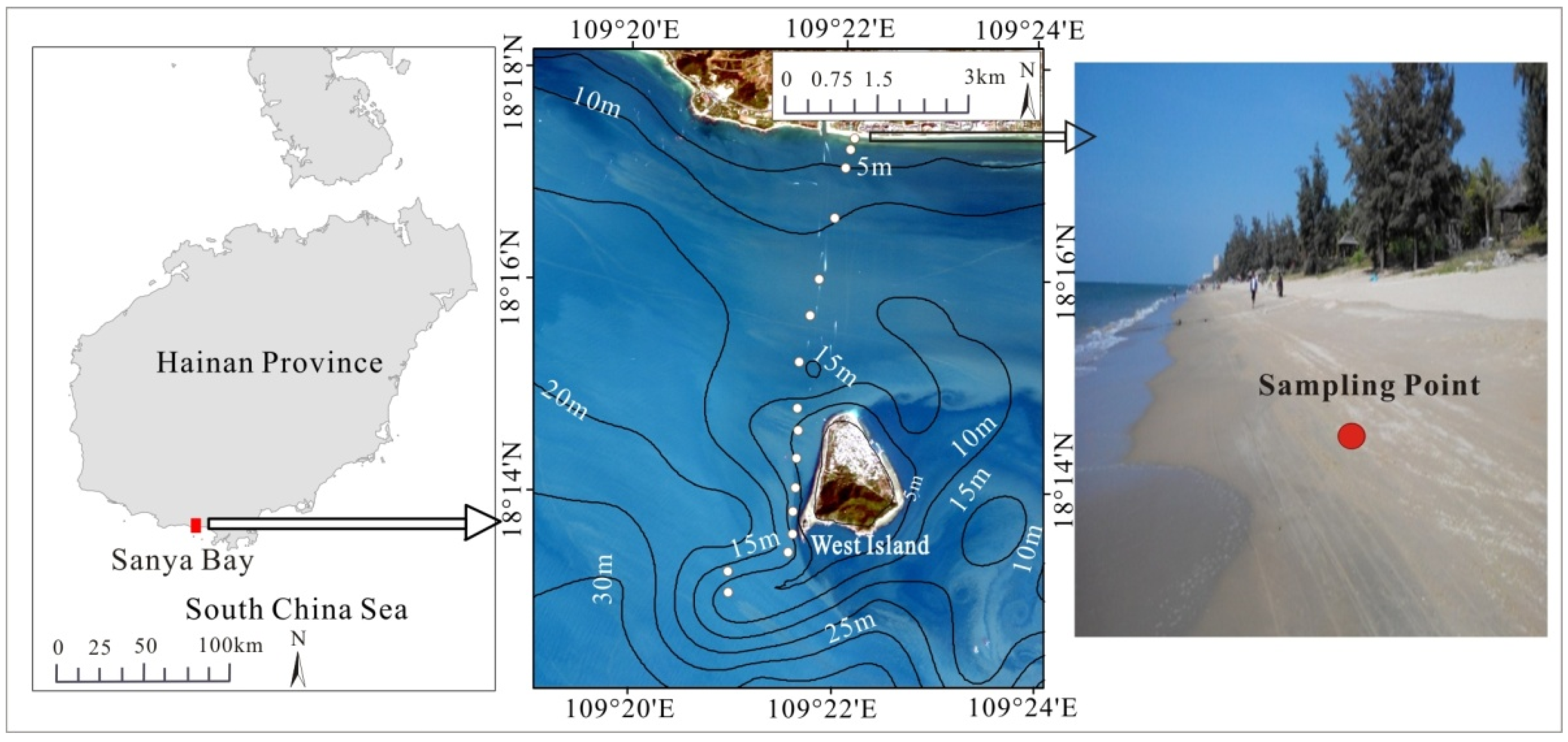
2.1. Study Area
2.2. SPOT6 Data
2.3. In Situ Measured Dataset
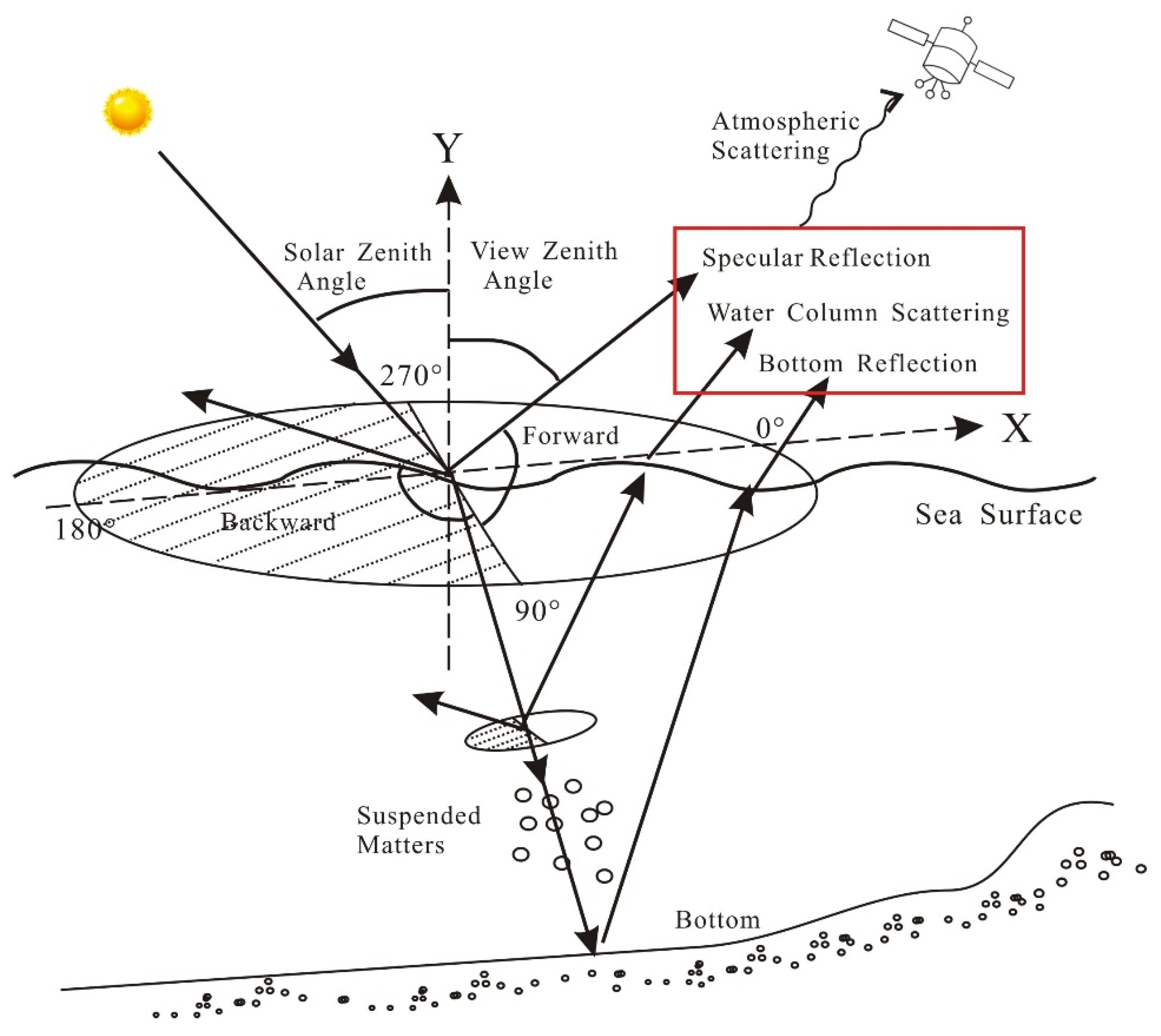
3. Remote Sensing Reflectance Algorithm
3.1. Sun Glint Effect
3.2. Water-Leaving Reflectance Contributed by Bottom Reflectance (Rbw)
4. Chl-a Concentration Retrieval Algorithm
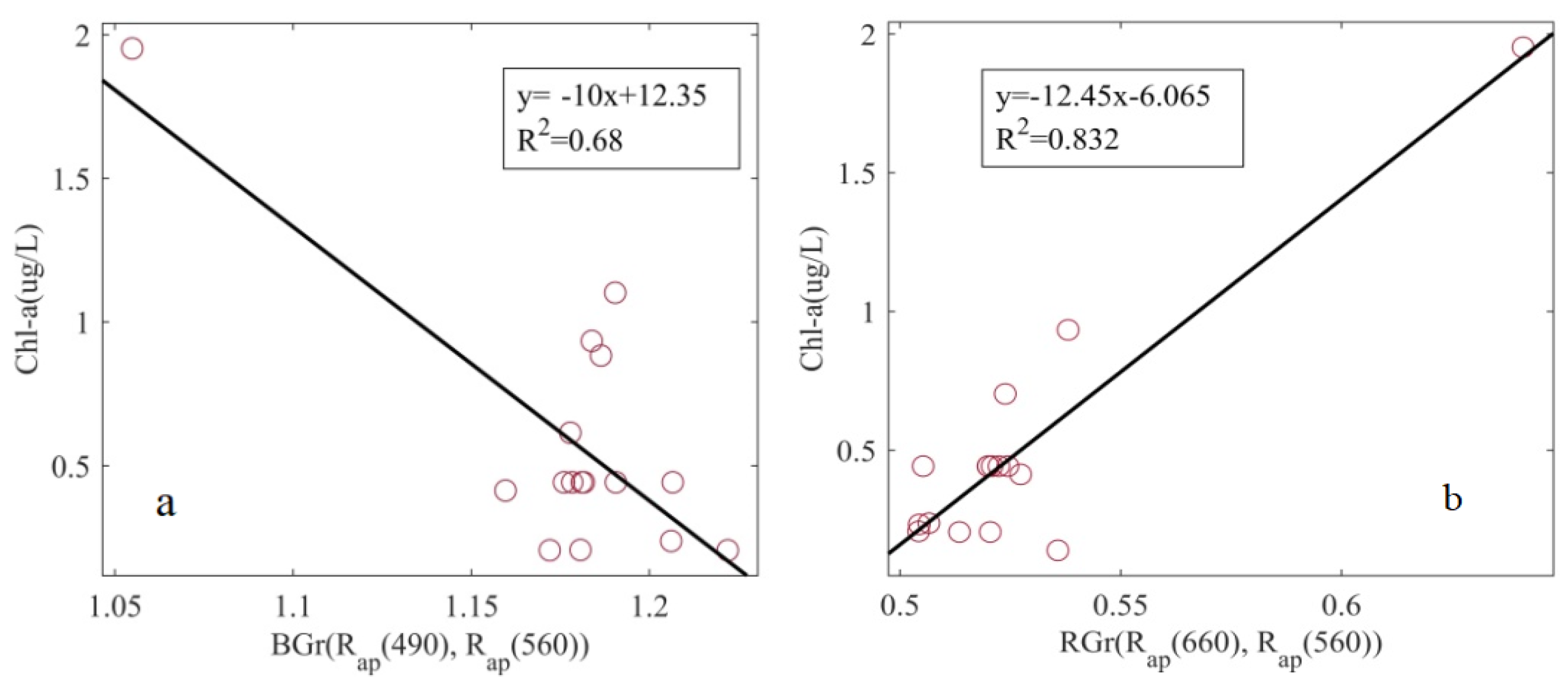
4.1. Review of the Chl-a Retrieval Algorithm
4.2. Improved Chl-a Concentration Algorithm
5. Results
5.1. SPOT6 Data Atmospheric Correction
5.2. Parameter u(λ) Correction
5.3. Comparison of the Different Algorithms
5.4. Statistical Analysis
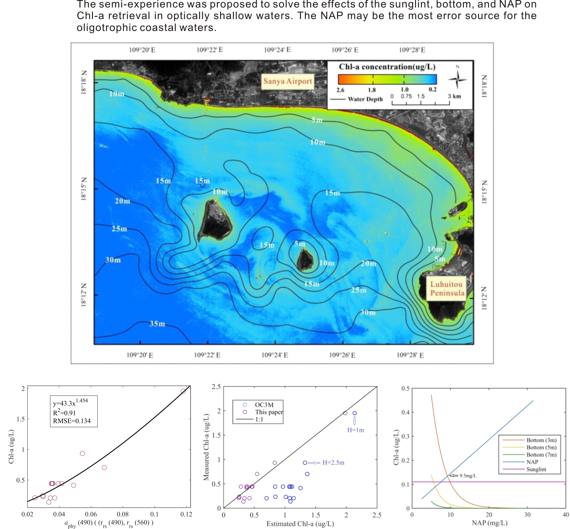
5.5. Sun Glint Effect
5.6. Bottom Effect
5.7. The Effect of NAP on Spatial Distribution
5.8. Chl-a Retrieval of SYB
6. Discussion
7. Conclusions
Author Contributions
Funding
Acknowledgments
Conflicts of Interest
Appendix A
Appendix A.1. The Relative Spectral Response Function (RSRF) of SPOT6 Data

Appendix A.2. Diffuse Attenuation Coefficient
Appendix A.3. Estimating the NAP Concentration

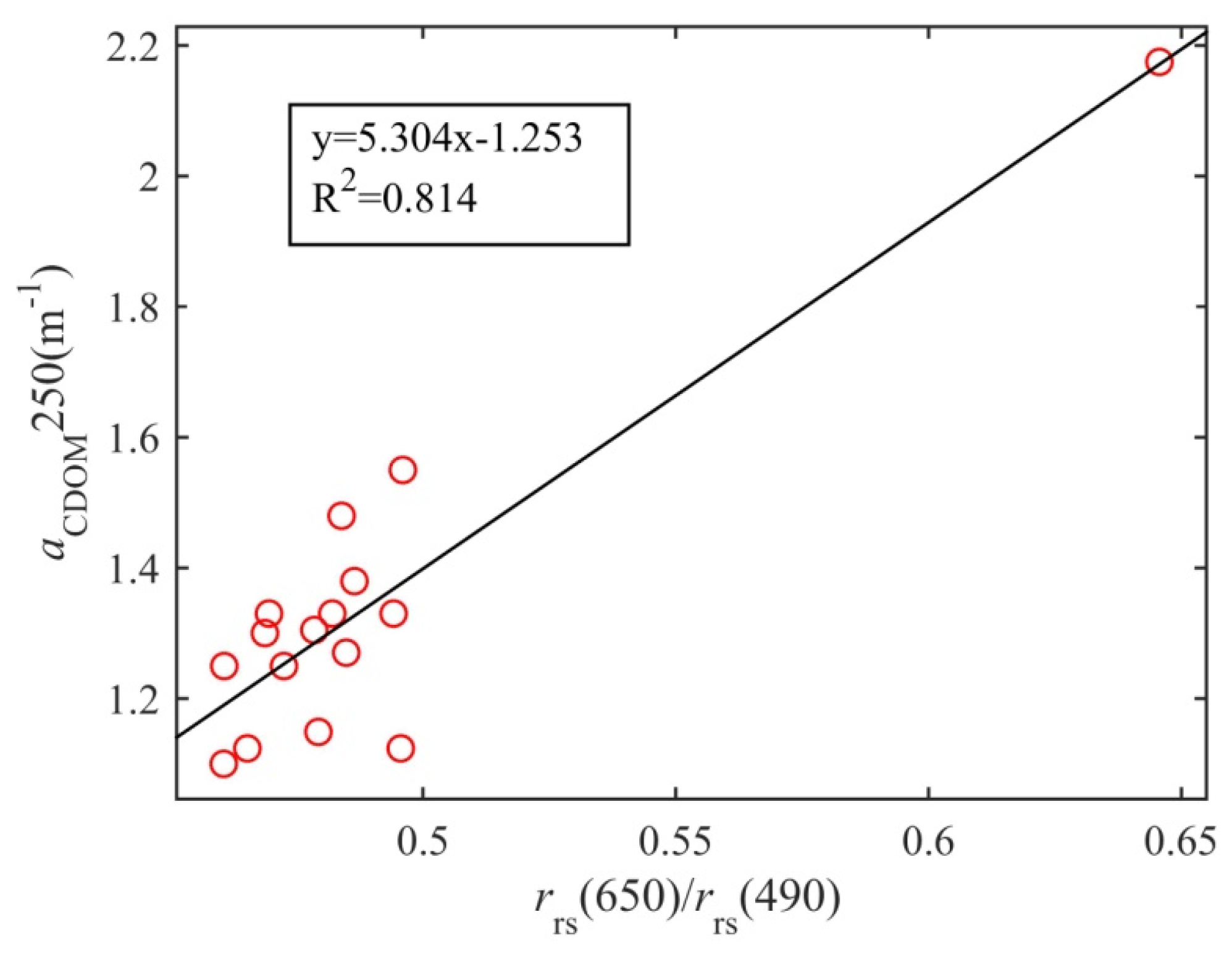
Appendix A.4. Absorption Coefficient of the Colored Dissolved Organic Matter (CDOM) Estimation

References
- Mcgranahan, G.; Balk, D.; Anderson, B. The Rising Tide: Assessing the Risks of Climate Change and Human Settlements in Low Elevation Coastal Zones. Environ. Urban. 2007, 19, 17–37. [Google Scholar] [CrossRef]
- Blondeau-Patissier, D.; Gower, J.F.R.; Dekker, A.G.; Phinn, S.R.; Brando, V.E. A Review of Ocean Color Remote Sensing Methods and Statistical Techniques for the Detection, Mapping and Analysis of Phytoplankton Blooms in Coastal and Open Oceans. Prog. Oceanogr. 2014, 123, 123–144. [Google Scholar] [CrossRef] [Green Version]
- Yu, Y.; Chen, S.; Lu, T.Q.; Tian, S. Coastal Disasters and Remote Sensing Monitoring Methods. In Sea Level Rise and Coastal Infrastructure, 1st ed.; Zhang, Y.Z., Hou, Y.J., Eds.; IntechOpen: London, UK, 2018; pp. 119–138. [Google Scholar] [CrossRef] [Green Version]
- Gordon, H.R.; Morel, A.Y. Remote Assessment of Ocean Color for Interpretation of Satellite Visible Imagery. In A Review Lecture Notes on Coastal and Estuarine Studies; Springer: New York, NY, USA, 1983; Volume 4, p. 114. [Google Scholar]
- Morel, A. Optical Modeling of the Upper Ocean in Relation to its Biogenous Matter Content (Case-1 Waters). J. Geophys. Res. Oceans 1988, 93, 10749–10768. [Google Scholar] [CrossRef] [Green Version]
- Aiken, J.; Moore, G.F.; Trees, C.C.; Hook, S.B.; Clark, D.K. The SeaWiFS CZCS-type pigment algorithm. In SeaWiFS Technical Report Series; Goddard Space Flight Center: Greenbelt, MD, USA, 1995. [Google Scholar]
- Carder, K.L.; Chen, F.R.; Cannizzaro, J.P.; Campbell, J.W.; Mitchell, B.G. Performance of the MODIS Semi-analytical Ocean Color Algorithm for Chlorophyll-a. Adv. Space Res. 2004, 33, 1152–1159. [Google Scholar] [CrossRef]
- Ha, N.T.T.; Koike, K.; Nhuan, M.T. Improved Accuracy of Chlorophyll-a Concentration Estimates from MODIS Imagery Using a Two-Band Ratio Algorithm and Geostatistics: As Applied to the Monitoring of Eutrophication Processes over Tien Yen Bay (Northern Vietnam). Remote Sens. 2014, 6, 421–442. [Google Scholar] [CrossRef] [Green Version]
- Gordon, H.R.; Clark, D.K.; Brown, J.W.; Brown, O.B.; Evans, R.H. Phytoplankton Pigment Concentrations in the Middle Atlantic Bight: Comparison of Ship Determinations and CZCS Estimates. Appl. Opt. 1983, 22, 20–36. [Google Scholar] [CrossRef]
- O’Reilly, J.E.; Maritorena, S.; Mitchell, B.G.; Siegel, D.A.; Carder, K.L.; Garver, S.A.; Kahru, M.; McClain, C. Ocean Color Chlorophyll Algorithms for SeaWiFS. J. Geophys. Res. 1998, 103, 24937–24953. [Google Scholar] [CrossRef] [Green Version]
- O’Reilly, J.E.; Maritorena, S.; Mitchell, B.G.; Siegel, D.A.; Carder, K.L.; Garver, S.A.; Kahru, M.; McClain, C. Ocean Color Chlorophyll a Algorithms for SeaWiFS, OC2, and OC4: Version 4. In SeaWiFS Postlaunch Calibration and Validation Analyses, Part 3, SeaWiFS Postlaunch Technical Report Series; Hooker, S.B., Firestone, E.R., Eds.; NASA Goddard Space Flight Center: Greenbelt, MD, USA, 2000; Volume 11, pp. 9–23. [Google Scholar]
- Carder, K.L.; Chen, F.R.; Lee, Z.P.; Hawes, S.K.; Cannizzaro, J.P. MODIS Ocean Science Team Algorithm Theoretical Basis Document, ATBD 19, Case 2 Chlorophyll-a, Version 7. Available online: http://modis.gsfc.nasa.gov/data/atbd/atbd_mod19.pdf.2003 (accessed on 6 June 2014).
- Thu, H.N.T.; Phuong, T.N.T.; Katsuaki, K.; Trong, N.M. Selecting the Best Band Ratio to Estimate Chlorophyll-a Concentration in a Tropical Freshwater Lake Using Sentinel 2a Images from a Case Study of Lake Ba Be (Northern Vietnam). ISPRS Int. J. Geo-Inf. 2017, 6, 290. [Google Scholar]
- Liu, G.; Li, L.; Song, K.S.; Li, Y.M.; Lyu, H.; Wen, Z.; Fang, C.; Bi, S.; Sun, X.; Wang, Z.; et al. An OLCI-based Algorithm for Semi-Empirically Partitioning Absorption Coefficient and Estimating Chlorophyll a Concentration in Various Turbid Case-2 Waters. Remote Sens. Environ. 2020, 239. [Google Scholar] [CrossRef]
- Lee, Z.P.; Carder, K.L.; Arnone, R.A. Deriving Inherent Optical Properties from Water Color: A Multiband Quasi-analytical Algorithm for Optically Deep Waters. Appl. Opt. 2002, 41, 5755–5772. [Google Scholar] [CrossRef]
- Chen, J.; Zhang, X.; Quan, W. Retrieval Chlorophyll-a Concentration from Coastal Waters: Three-band Semi-Analytical Algorithms Comparison and Development. Opt. Express 2013, 21, 9024–9042. [Google Scholar] [CrossRef] [PubMed]
- Chen, J.; Quan, W.; Wen, Z.; Cui, T. An Improved Three-band Semi-analytical Algorithm for Estimating Chlorophyll-a Concentration in Highly Turbid Coastal Waters: A Case Study of the Yellow River Estuary, China. Environ. Earth Sci. 2013, 69, 2709–2719. [Google Scholar] [CrossRef]
- Gitelson, A.A.; Dall’Olmo, G.; Moses, W.; Rundquist, D.C.; Barrow, T.; Fisher, T.R.; Gurlin, D.; Holz, J. A Simple Semi-Analytical Model for Remote Estimation of Chlorophyll-a in Turbid Waters: Validation. Remote Sens. Environ. 2008, 112, 3582–3593. [Google Scholar] [CrossRef]
- Matthews, M.W.; Bernard, S.; Winter, K. Remote Sensing of Cyanobacteria-Dominant Algal Blooms and Water Quality Parameters in Zeekoevlei, a Small Hypertrophic Lake, Using MERIS. Remote Sens. Environ. 2010, 114, 2070–2087. [Google Scholar] [CrossRef]
- Gilerson, A.A.; Gitelson, A.A.; Zhou, J.; Gurlin, D.; Moses, W.; Ioannou, I.; Ahmed, S.A. Algorithms for Remote Estimation of Chlorophyll-a in Coastal and Inland Waters Using Red and Near-infrared Bands. Opt. Express 2010, 18, 24109–24125. [Google Scholar] [CrossRef] [PubMed] [Green Version]
- Toming, K.; Kutser, T.; Laas, A.; Sepp, M.; Paavel, B.; Nõges, T. First Experiences in Mapping Lake Water Quality Parameters with Sentinel-2 MSI Imagery. Remote Sens. 2016, 8, 640. [Google Scholar] [CrossRef] [Green Version]
- Dahanayaka, D.D.G.L.; Tonooka, H.; Wijeyaratne, M.J.S.; Minato, A.; Ozawa, S. Two Decadal Trends of Surface Chlorophyll-a Concentrations in Tropical Lagoon Environments in Sri Lanka Using Satellite and In-situ data. Asian J. Geoinform. 2013, 13, 7–16. [Google Scholar]
- Fernanda, W.; Enner, A.; Thanan, R.; Nilton, I.; Cláudio, B.; Luiz, R. Estimation of Chlorophyll-a Concentration and the Trophic State of the Barra Bonita Hydroelectric Reservoir Using OLI/Landsat-8 Images. Int. J. Environ. Res. Public Health 2015, 12, 10391–10417. [Google Scholar] [CrossRef]
- Ha, N.T.T.; Koike, K.; Nhuan, M.T.; Canh, B.D.; Thao, N.T.P.; Parsons, M. Landsat 8/OLI Two Bands Ratio Algorithm for Chlorophyll-a Concentration Mapping in Hypertrophic Waters: An Application to West Lake in Hanoi (Vietnam). IEEE J. Sel. Top. Appl. Earth Obs. Remote Sens. 2017, 10, 4919–4929. [Google Scholar] [CrossRef]
- Cox, C.; Munk, W. Statistics of the Sea Surface Derived from Sun Glitter. J. Mar. Res. 1954, 13, 198–227. [Google Scholar]
- Cox, C.; Munk, W. Slopes of the Sea Surface Deduced from Photographs of Sun Glitter. Bull Scripps Inst. Oceanogr. Univ. Calif. 1956, 6, 401–488. [Google Scholar]
- Zhang, H.; Wang, M. Evaluation of Sun Glint Models Using MODIS Measurements. J. Quant. Spectrosc. Radiat. Transf. 2010, 111, 492–506. [Google Scholar] [CrossRef]
- Zhang, H.; Yang, K.; Lou, X.; Li, Y.; Zheng, G.; Wang, J.; Wang, X.; Ren, L.; Li, D.; Shi, A. Observation of Sea Surface Roughness at a Pixel Scale Using Multi-angle Sun Glitter Images Acquired by the ASTER Sensor. Remote Sens. Environ. 2018, 208, 97–108. [Google Scholar] [CrossRef]
- Hu, C. An Empirical Approach to Derive MODIS Ocean Color Patterns under Severe Sun Glint. Geophys. Res. Lett. 2011, 38. [Google Scholar] [CrossRef]
- Harmel, T.; Chami, M.; Tormos, T.; Reynaud, N.; Danis, P.A. Sunglint Correction of the Multi-Spectral Instrument (MSI)-Sentinel-2 Imagery over inland and Sea Waters from SWIR Bands. Remote Sens. Environ. 2017, 204, 308–321. [Google Scholar] [CrossRef]
- Hlaing, S.; Gilerson, A.; Harmel, T.; Tonizzo, A.; Weidemann, A.; Arnone, R.; Ahmed, S. Assessment of a Bidirectional Reflectance Distribution Correction of above Water and Satellite Water-Leaving Radiance in Coastal Waters. Appl. Opt. 2012, 51, 220–237. [Google Scholar] [CrossRef] [Green Version]
- Lee, Z.; Carder, K.L.; Mobley, C.D.; Steward, R.G.; Patch, J.S. Hyperspectral Remote Sensing for Shallow Waters: 2. Deriving Bottom Depths and Water Properties by Optimization. Appl. Opt. 1999, 38, 3831–3843. [Google Scholar] [CrossRef] [Green Version]
- Lee, Z.; Carder, K.L.; Hawes, S.K.; Steward, R.G.; Peacock, T.G.; Davis, C.O. Model for the Interpretation of Hyperspectral Remote-Sensing Reflectance. Appl. Opt. 1994, 33, 5721–5732. [Google Scholar] [CrossRef] [Green Version]
- Lee, Z.; Carder, K.L.; Mobley, C.D.; Steward, R.G.; Patch, J.S. Hyperspectral Remote Sensing for Shallow Waters: 1. A Semianalytical Model. Appl. Opt. 1998, 37, 6329–6338. [Google Scholar] [CrossRef]
- Albert, A.; Mobley, C. An Analytical Model for Subsurface Irradiance and Remote Sensing Reflectance in Deep and Shallow Case-2 Waters. Opt. Express 2003, 11, 2873–2890. [Google Scholar] [CrossRef]
- Conrad, C.; Fritsch, S.; Zeidler, J.; Rucker, G.; Dech, S. Per-Field Irrigated Crop Classification in Arid Central Asia Using SPOT and ASTER Data. Remote Sens. 2010, 2, 1035–1056. [Google Scholar] [CrossRef] [Green Version]
- Ali, H.T.O.; Niculescu, S.; Sellin, V.; Bougault, C. Contribution of the New satellites (Sentinel-1, Sentinel-2, and SPOT-6) to the Coastal Vegetation Monitoring in the Pays de Brest (France). In Remote Sensing for Agriculture, Ecosystems, and Hydrology XIX; International Society for Optics and Photonics: Bellingham, WA, USA, 2017; Volume 10421, p. 1042129. [Google Scholar]
- Motlagh, M.G.; Kafaky, S.B.; Mataji, A.; Akhavan, R. Estimating and Mapping Forest Biomass Using Regression Models and SPOT-6 Images (Case Study: Hyrcanian Forests of North of Iran). Environ. Monit. Assess. 2018, 190, 352. [Google Scholar] [CrossRef] [PubMed]
- Ritchie, J.C.; Zimba, P.V.; Everitt, J.H. Remote Sensing Techniques to Assess Water Quality. Photogramm. Eng. Remote Sens. 2003, 69, 695–704. [Google Scholar] [CrossRef] [Green Version]
- Dekker, A.G.; Peters, S.W.M. The use of the Thematic Mapper for the Analysis of Eutrophic Lakes: A case Study in the Netherlands. Int. J. Remote Sens. 1993, 14, 799–821. [Google Scholar] [CrossRef]
- Ritchie, J.C.; Schiebe, F.R.; Cooper, C.M.; Harrington, J.A. Chlorophyll Measurements in the Presence of Suspended Sediment Using Broad Band Spectral Sensors Aboard Satellites. J. Freshw. Ecol. 1994, 9, 197–206. [Google Scholar] [CrossRef]
- The Free Dictionary by FARLEX, Sanya. Available online: https://encyclopedia.thefreedictionary.com/Sanya (accessed on 6 June 2014).
- Li, S.J.; Li, Y.W.; Fan, B.; Gao, X.M.; Xu, X.Q.; Teng, Y.; Ye, Q. Wave Observation and Statistical Analysis in the Southeast Coast of Hainan Island. Adv. Mar. Sci. 2016, 34, 2–9. [Google Scholar]
- Bricaud, A.; Stramski, D. Spectral Absorption Coefficients of Living Phytoplankton and Non-Algal Biogenous Matter: A comparison Between the Peru Upwelling Area and the Sargasso Sea. Limnol. Oceanogr. 1990, 35, 562–582. [Google Scholar] [CrossRef]
- Xi, H.Y.; Larouche, P.; Michlel, C.; Tang, S.L. Beam Attenuation, Scattering and Backscattering of Marine Particles in relation to Particle Size Distribution and Composition in Hudson Bay (Canada). J. Geophys. Res. Oceans 2015, 120, 3286–3300. [Google Scholar] [CrossRef] [Green Version]
- Neil, C.; Cunningham, A.; Mckee, D. Relationships between Suspended Mineral Concentrations and Red-Waveband Reflectances in Moderately Turbid Shelf Seas. Remote Sens. Environ. 2011, 115. [Google Scholar] [CrossRef]
- Whitmire, A.L.; Pegau, W.S.; Lee, K.B.; Boss, B.; Cowles, T.J. Spectral Backscattering Properties of Marine Phytoplankton Cultures. Opt. Express 2010, 18, 15073–15093. [Google Scholar] [CrossRef] [Green Version]
- Mobley, C.D. Estimation of the Remote-Sensing Reflectance from Above-Surface Measurements. Appl. Opt. 1999, 38, 7442–7455. [Google Scholar] [CrossRef] [PubMed]
- Zhang, H.; Voss, K.J. Bidirectional Reflectance Measurements of Sediments in The Vicinity of Lee Stocking Island, Bahamas. Limnol. Oceanogr. 2013, 48, 380–389. [Google Scholar] [CrossRef]
- Hu, C.; Muller-Karger, F.E.; Taylor, C.; Carder, K.L.; Kelble, C.; Johns, E.; Heil, C.A. Red Tide Detection and Tracing Using MODIS Fluorescence Data: A Regional Example in SW Florida Coastal Waters. Remote Sens. Environ. 2005, 97, 311–321. [Google Scholar] [CrossRef]
- Hu, C.; Lee, Z.; Franz, B. Chlorophyll-a Algorithms for Oligotrophic Oceans: A Novel Approach Based on Three-Band Reflectance Difference. J. Geophys. Res. Oceans. 2012, 117. [Google Scholar] [CrossRef] [Green Version]
- Gower, J.; King, S.; Yan, W.; Borstad, G.; Brown, L. Use of the 709 nm Band of MERIS to Detect Intense Plankton Blooms and Other Conditions in Coastal Waters. Eur. Space Agency 2005, 31. [Google Scholar]
- Gitelson, A.A.; Guilin, D.; Moses, W.J.; Barrow, T. A Bio-Optical Algorithm for the Remote Estimation of the Chlorophyll-A Concentration in Case 2 Waters. Environ. Res. Lett. 2009, 4, 045003. [Google Scholar] [CrossRef]
- Gordon, H.R.; Brown, J.W.; Brown, O.B.; Evans, R.H.; Smith, R.C. A Semi-Analytic Radiance Model of Ocean Color. J. Geophys. Res. Atmos. 1988, 93, 10909–10924. [Google Scholar] [CrossRef]
- Park, Y.J.; Ruddick, K. Model of remote-sensing reflectance including bidirectional effects for case 1 and case 2 waters. Appl. Opt. 2005, 44, 1236–1249. [Google Scholar] [CrossRef]
- Stramski, D.; Bricaud, A.; Morel, A. Modeling the Inherent Optical Properties of the Ocean Based on the Detailed Composition of the Planktonic Community. Appl. Opt. 2001, 40, 2929–2945. [Google Scholar] [CrossRef]
- Mitchell, B.G.; Kahru, M.; Wieland, J. Determination of Spectral Absorption Coefficients of Particles, Dissolved Material and Phytoplankton for Discrete Water Samples. Ocean Opt. Protoc. Satell. Ocean Color Sens. Valid. Revis. 2002, 3, 231–257. [Google Scholar]
- Smith, R.C.; Baker, K.S. Optical Properties of the Clearest Natural Waters (200–800 nm). Appl. Opt. 1981, 20, 177–184. [Google Scholar] [CrossRef] [PubMed]
- Twardowski, M.S.; Claustre, H.; Freeman, S.A.; Stramski, D.; Huot, Y. Optical Backscattering Properties of the “Clearest” Natural Waters. Biogeosciences 2007, 4, 1041–1058. [Google Scholar] [CrossRef] [Green Version]
- Antoite, D.; Andre, J.M.; Morel, A. Oceanic Primary Production 2: Estimation of Global Scale from Satellite (Coastal Zone Color Scanner) Chlorophyll. Glob. Biogeochem. Cy. 1996, 10, 57–69. [Google Scholar] [CrossRef]
- McKee, D.; Cunningham, A.; Slater, J.; Jones, K.J.; Griffiths, C.R. Inherent and Apparent Optical Properties in Coastal Waters: A study of the Clyde Sea in Early Summer. Estuar. Coast. Shelf Sci. 2002, 56, 369–376. [Google Scholar] [CrossRef]
- McKee, D.; Cunningham, A. Identification and Characterization of Two Optical Water Types in the Irish Sea from in Situ Inherent Optical Properties and Seawater Constituents. Estuar. Coast. Shelf Sci. 2006, 68, 305–316. [Google Scholar] [CrossRef]
- Pope, R.M.; Fry, E.S. Absorption Spectrum (380–700 nm) of Pure Water II. Integrating Cavity Measurements. Appl. Opt. 1997, 36, 8710–8723. [Google Scholar] [CrossRef]
- Wang, M. A Sensitivity Study of the SeaWiFS Atmospheric Correction Algorithm: Effects of Spectral Band Variations. Remote Sens. Environ. 1999, 67, 348–359. [Google Scholar] [CrossRef]
- Adler-Golden, S.M.; Matthew, M.W.; Bernstein, L.S.; Levine, R.Y.; Berk, A.; Richtsmeier, S.C.; Acharya, P.K.; Anderson, G.P.; Felde, G.; Gardner, J.; et al. Atmospheric Correction for Short Wave Spectral Imagery Based on MODTRAN4. SPIE Proc. Imaging Spectr. 1999, 3753, 61–69. [Google Scholar]
- Vis, I. Atmosphere Correction Module: QUAC and FLAASH User’s Guide. In ITT Visual Information Solutions, 4th ed.; ITT: Boulder, CO, USA, 2009. [Google Scholar]
- Rotta, L.H.S.; Alcantara, E.H.; Watanabe, F.S.Y.; Rodrigues, T.W.P.; Imai, N.N. Atmospheric Correction Assessment of SPOT-6 Image and its Influence on Models to Estimate Water Column Transparency in Tropical Reservoir. Remote Sens. Appl. Soc. Environ. 2016, 4, 158–166. [Google Scholar] [CrossRef]
- Lu, T.Q.; Chen, S.B.; Tu, Y.; Yu, Y.; Cao, Y.J.; Jiang, D.Y. Comparative Study on Coastal Depth Inversion Based on Multi-source Remote Sensing Data. Chin. Geogr. Sci. 2019, 29, 192–201. [Google Scholar] [CrossRef] [Green Version]
- Chen, Q.D.; Deng, R.R.; QIN, Y.; Xiong, L.H.; He, Y.Q. Analysis of Spectral Characteristics of Coral Under Different Growth Patterns. Acta Ecol. Sin. 2015, 35, 3394–3402. [Google Scholar]
- Carlson, R.E. A Trophic State Index for Lakes. Limnol. Oceanogr. 1977, 22, 361–369. [Google Scholar] [CrossRef] [Green Version]
- Lamparelli, M.C. Graus De Trofia Em Corpos D’Água Do Estado De São Paulo. Ph.D. Thesis, University of São Paulo, São Paulo, Brazil, 2004. [Google Scholar]
- Ocean Color Web. Available online: http://oceancolor.gsfc.nasa.-gov/ANALYSIS/ocv6/ (accessed on 6 June 2014).
- Tassan, S. Local Algorithms Using SeaWiFS data for the Retrieval of Phytoplankton, Pigments, Suspended Sediment, and Yellow Substance in Coastal Waters. Appl. Opt. 1994, 33, 2369–2378. [Google Scholar] [CrossRef] [PubMed]
- Kallio, K. Optical Properties of Finnish Lakes Estimated with Simple Bio-Optical Models and Water Quality Monitoring Data. Hydrol. Res. 2006, 37, 183–204. [Google Scholar] [CrossRef]
- Brezonik, P.; Olmanson, L.; Finlay, J.; Bauer, M. Factors Affecting the Measurement of CDOM by Remote Sensing of Optically Complex Inland Waters. Remote Sens. Environ. 2015, 157, 199–215. [Google Scholar] [CrossRef]
- Ana, R.; Martin, H.; Gonzalo, M.G.; Sampsa, K.; Kari, K.; Gustau, C.V. Machine Learning Regression Approaches for Colored Dissolved Organic Matter (CDOM) Retrieval with S2-MSI and S3-OLCI Simulated Data. Remote Sens. 2018, 10, 786. [Google Scholar]
- Bricaud, A.; Morel, A.; Prieur, L. Absorption by Dissolved Organic Matter of the Sea (YELLOW SUBSTANCE) in the UV and Visible Domains. Limnol. Oceanogr. 1981, 26, 43–53. [Google Scholar] [CrossRef]
- Song, K.S.; Shang, Y.X.; Wen, Z.D.; Jacinthe, P.A.; Liu, G.; Lyu, L.L.; Fang, C. Characterization of CDOM in Saline and Freshwater Lakes Across China Using Spectroscopic Analysis. Water Res. 2019, 150, 403–417. [Google Scholar] [CrossRef] [Green Version]


| Wavelength (nm) | aphy (m−1) | aNAP (m−1) | aCDOM (m−1) | aw (m−1) | bb*NAP (m2 g−1) | Chl-a (ug/L) | NAP (mg/L) | H (m) | |
|---|---|---|---|---|---|---|---|---|---|
| mean | 490 | 0.034 | 0.1 | 0.037 | 0.019 | 0.0156 | 0.587 | 5.565 | 7.803 |
| 560 | 0.011 | 0.076 | 0.013 | 0.071 | 0.0150 | ||||
| 660 | 0.017 | 0.033 | 0.003 | 0.410 | 0.0141 | ||||
| max | 490 | 0.171 | 0.562 | 0.059 | - | 1.952 | 23.570 | 15.000 | |
| 560 | 0.039 | 0.218 | 0.021 | - | |||||
| 660 | 0.063 | 0.151 | 0.005 | - | |||||
| min | 490 | 0.023 | 0.02 | 0 | - | 0.205 | 2.670 | 1.0 | |
| 560 | 0.006 | 0.012 | 0 | - | |||||
| 660 | 0.011 | 0.006 | 0 | - |
| Symbols and Abbreviations | Description | Units |
|---|---|---|
| aw | Absorption coefficient of pure water | m−1 |
| aphy | Absorption coefficient of algal pigments | m−1 |
| aNAP | Absorption coefficient of non-algal pigments | m−1 |
| aCDOM | Absorption coefficient of CDOM | m−1 |
| a | Absorption coefficient of the total (=aw + aphy + aNAP + aCDOM) | m−1 |
| b | Scattering coefficients | m−1 |
| B | Backscattering ratio | |
| bb | Backscattering coefficients | m−1 |
| Chl-a | Chlorophyll-a concentration | ug/L |
| β(ψ,λ) | Volume scattering function (VSF) | |
| f/Q | Water column bidirectional factor | sr−1 |
| D | Bottom slope | deg |
| D′ | Bottom aspect | deg |
| H | Water depth | m |
| tgas(λ) | Gaseous transmittance | m−1 |
| t(λ) | Total diffuse atmospheric transmission | m−1 |
| ρt(λ) | Irradiance reflectance just above the water surface | |
| ρA(λ) | Aerosol reflectance | |
| ρr(λ) | Molecular Rayleigh scattering reflectance | |
| Rrs | Remote sensing reflectance | sr−1 |
| Rap | Apparent remote sensing reflectance | sr−1 |
| Rsg | Surface specular reflectance | sr−1 |
| Rcw | Remote sensing reflectance from water-column scattering | sr−1 |
| Rbw | Remote sensing reflectance from bottom reflectance | sr−1 |
| θ0 | Solar zenith angle above water surface | deg |
| θ | View angle above the water surface | deg |
| θ0′ | Subsurface solar zenith angle | deg |
| θ′ | Subsurface view zenith angle | deg |
| θn | Water surface slope gradient | deg |
| μ0 | Cosine of θ0 | |
| μ | Cosine of θ | |
| μn | Cosine of θn | |
| tu | Water–air transmittance | sr−1 |
| td | Air–water transmittance | sr−1 |
| L | Optical path-elongation factor | m−1 |
| k | Beam attenuation coefficient (=a + bb) | m−1 |
| φ | Relative azimuth angle | de |
| Θ | Sun–satellite relative phase angle | deg |
| σu | Mean square slope in an upwind direction | deg |
| σc | Mean square slop in the crosswind direction | deg |
| λ | Wavelength | nm |
| W | Wind speed | m/s |
| △φ | Wind direction | deg |
| n | Water refractive index (≈1.34 in seawater) | |
| SYB | Sanya Bay | |
| CDOM | Coloured dissolved organic matter | m−1 |
| Chl-a | Chlorophyll-a | |
| CZCS | Coastal zone color scanner | |
| IOPs | Inherent optical properties | |
| MODIS | Moderate resolution imaging spectroradiometer | |
| 2Br | Two-band-ratio | |
| BGr | Blue-green band-ratio | |
| DCI | Difference Chl-a index | |
| NAP | Suspended mineral particle | mg/L |
| NIR | Near-infrared | |
| NRr | NIR-red band-ratio | |
| RGr | Red-green band–ratio | |
| RSRF | Relative spectral response function | |
| RTM | Radiative transfer model | |
| SeaWiFS | Sea-viewing wide field of view sensor | |
| SAA | Solar azimuth angle | deg |
| SGR | Sun–satellite geometric relationship | deg |
| SZA | Solar zenith angle | deg |
| VZA | View zenith angle | deg |
| VAA | View azimuth angle | deg |
| Algorithm | Sensor | Band | Water Type | Reference |
|---|---|---|---|---|
| BGr | OLI | 483, 562 | Eutrophic inland | [23,24] |
| RGr | Sentinel-2 | 665, 560 | Eutrophic inland | [13] |
| OC3M | MODIS | 443, 488, 555 | Case-2 coastal | [12] |
| QAA | SeaWiFS | 443, 490, 550, 667 | Case-2 coastal | [10,11] |
| FLH | MODIS | 667, 678, 746 | Eutrophic coastal | [50] |
| CI | MERIS | 443, 555, 670 | Oligotrophic | [51] |
| MCI | MERIS | 681, 709, 753 | Eutrophic coastal | [52,53] |
| Sensor Type | SPOT 6 | Atmospheric Model | Tropical |
|---|---|---|---|
| Sensor altitude | 695 km | Aerosol model | Maritime |
| Ground elevation | 0 m | Initial visibility | 30 km |
| Flight data | 21 January 2013 | View zenith angle | 22° |
| Flight time | 10:58 | View azimuth angle | 135° |
| Algorithm | Data | Empirical Coefficients | R2 | RMSE | MAPE |
|---|---|---|---|---|---|
| BGr | Rap (λ) | y = 67.85x2 − 163.9x + 99.31 | 0.72 | 0.2255 | 41.72% |
| Y = −10x + 12.35 | 0.68 | 0.2565 | 66.23% | ||
| Rrs (λ) | y = 42.98x2 − 108.9 + 68.18 | 0.74 | 0.2243 | 36.28% | |
| y = −7.66x + 9.859 | 0.7 | 0.2444 | 50.46% | ||
| rrs (λ) | y = 47.85x2 − 116.9 + 71.78 | 0.75 | 0.2223 | 40.93% | |
| y = −7.57x + 9.5 | 0.72 | 0.2422 | 41.56% | ||
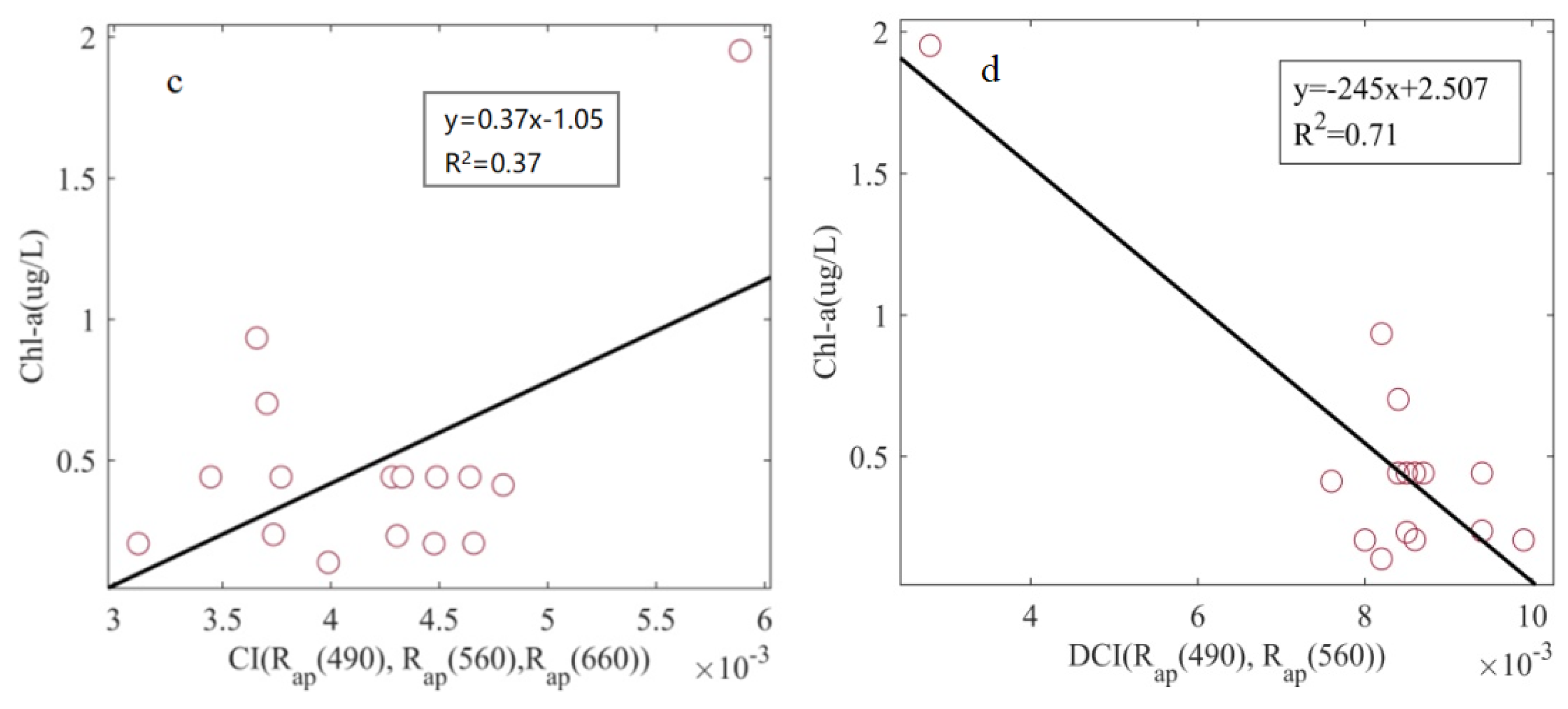
| DCI | Rap (λ) | y = −8901x2 − 1042x + 2.061 | 0.76 | 0.2151 | 36.09% |
| y=-245x + 2.507 | 0.71 | 0.2277 | 45.92% | ||
| Rrs (λ) | y = −8901x2 − 1025x + 2.04 | 0.76 | 0.2151 | 36.04% | |
| Y = −245x + 2.475 | 0.71 | 0.2277 | 45.76% | ||
| rrs (λ) | y = −4478x2 − 558.2x + 1.843 | 0.77 | 0.2141 | 36.15% | |
| y = −131.3x + 2.057 | 0.75 | 0.2253 | 38.97% | ||
| aphy (490) | rrs (λ) | y = 43.3x1.454 | 0.91 | 0.11 | 21.51% |
© 2020 by the authors. Licensee MDPI, Basel, Switzerland. This article is an open access article distributed under the terms and conditions of the Creative Commons Attribution (CC BY) license (http://creativecommons.org/licenses/by/4.0/).
Share and Cite
Yu, Y.; Chen, S.; Qin, W.; Lu, T.; Li, J.; Cao, Y. A Semi-Empirical Chlorophyll-a Retrieval Algorithm Considering the Effects of Sun Glint, Bottom Reflectance, and Non-Algal Particles in the Optically Shallow Water Zones of Sanya Bay Using SPOT6 Data. Remote Sens. 2020, 12, 2765. https://doi.org/10.3390/rs12172765
Yu Y, Chen S, Qin W, Lu T, Li J, Cao Y. A Semi-Empirical Chlorophyll-a Retrieval Algorithm Considering the Effects of Sun Glint, Bottom Reflectance, and Non-Algal Particles in the Optically Shallow Water Zones of Sanya Bay Using SPOT6 Data. Remote Sensing. 2020; 12(17):2765. https://doi.org/10.3390/rs12172765
Chicago/Turabian StyleYu, Yan, Shengbo Chen, Wenhan Qin, Tianqi Lu, Jian Li, and Yijing Cao. 2020. "A Semi-Empirical Chlorophyll-a Retrieval Algorithm Considering the Effects of Sun Glint, Bottom Reflectance, and Non-Algal Particles in the Optically Shallow Water Zones of Sanya Bay Using SPOT6 Data" Remote Sensing 12, no. 17: 2765. https://doi.org/10.3390/rs12172765