Long-Term Discharge Estimation for the Lower Mississippi River Using Satellite Altimetry and Remote Sensing Images


Deutsches Geodätisches Forschungsinsitut der Technischen Universität München (DGFI-TUM), Arcisstraße 21, 80333 München, Germany
*
Author to whom correspondence should be addressed.
Remote Sens. 2020, 12(17), 2693; https://doi.org/10.3390/rs12172693
Submission received: 26 June 2020
/
Revised: 5 August 2020
/
Accepted: 17 August 2020
/
Published: 20 August 2020
Abstract
:Despite increasing interest in monitoring the global water cycle, the availability of in situ gauging and discharge time series is decreasing. However, this lack of ground data can partly be compensated for by using remote sensing techniques to observe river stages and discharge. In this paper, a new approach for estimating discharge by combining water levels from multi-mission satellite altimetry and surface area extents from optical imagery with physical flow equations at a single cross-section is presented and tested at the Lower Mississippi River. The datasets are combined by fitting a hypsometric curve, which is then used to derive the water level for each acquisition epoch of the long-term multi-spectral remote sensing missions. In this way, the chance of detecting water level extremes is increased and a bathymetry can be estimated from water surface extent observations. Below the minimum hypsometric water level, the river bed elevation is estimated using an empirical width-to-depth relationship in order to determine the final cross-sectional geometry. The required flow gradient is derived from the differences between virtual station elevations, which are computed in a least square adjustment from the height differences of all multi-mission satellite altimetry data that are close in time. Using the virtual station elevations, satellite altimetry data from multiple virtual stations and missions are combined to one long-term water level time series. All required parameters are estimated purely based on remote sensing data, without using any ground data or calibration. The validation at three gauging stations of the Lower Mississippi River shows large deviations primarily caused by the below average width of the predefined cross-sections. At 13 additional cross-sections situated in wide, uniform, and straight river sections nearby the gauges the Normalized Root Mean Square Error (NRMSE) varies between 10.95% and 28.43%. The Nash-Sutcliffe Efficiency (NSE) for these targets is in a range from 0.658 to 0.946.
Keywords:
river discharge; satellite altimetry; remote sensing; bathymetry; Manning; roughness; flow gradient; DAHITI
1. Introduction
Water is essential for all aspects of life on Earth and the global water cycle influences the climate decisively. In particular, freshwater is elementary as people’s livelihood. While rivers store only 0.006% of the global freshwater resources, they are the main source for freshwater consumption and irrigation [1]. With growing needs of the Earth’s increasing population and growing attention of climate change, water management developments are required to be sustainable. River discharge measurements provide the foundation for water resource planning, decision making, and design and operation of related infrastructure [2]. Moreover, they are of extreme importance for monitoring hydrological change in space and time. As discharge combines a variety of different flow and transfer processes within the up-stream catchment, it is an essential hydrological variable widely used for tuning and calibrating hydrological models [3]. Such models help to increase our knowledge about the global water cycle. While the water cycle is affected by global warming, it also influences the climate. As water cycles between the land, oceans, and atmosphere, it changes the dynamics and thermodynamics of the climate system [4].
In situ discharge is usually calculated using the water level measured at a gauge and a functional relation (rating curve), which is calibrated and regularly adjusted by in situ velocity measurements and depth soundings [5,6]. Establishing and maintaining such a discharge station is an involved and complicated process, which is cost- and time-intensive [7]. Thus, despite the need for increased attention to the global water cycle and freshwater resources, the number of freely available in situ discharge time-series in public databases such as the Global Runoff Data Centre (GRDC) is rapidly declining since about 1980, especially in remote areas outside Europe or the USA [8]. Therefore, there is a strong motivation to estimate discharge with remote sensing techniques.
In contrast to discharge, which cannot be measured directly from remote sensing data [9], many hydrological and hydraulic variables such as inundated area [10], lake surface area [11,12], and river widths [13,14,15] can be measured reliably with multispectral or hyperspectral sensors on board of satellites [16,17], such as the MODIS, Landsat, and Sentinel-2 satellites. In addition to the widely used sensors covering the visible and infrared spectrum, water surface area can also be acquired using other techniques such as SAR or passive microwave radiometers [16,18]. Although intended to monitor oceans, satellite altimetry can presently be used to measure water levels of inland water bodies such as lakes and reservoirs [19,20,21,22]. Furthermore, satellite altimetry is capable of measuring the water level and longitudinal topography of rivers wider than 200 m [23,24]. Combining water level and surface area data, reservoir bathymetry and storage variations can be derived but are limited by the minimum observed water level [25,26]. Rating curves between previously sampled in situ discharge measurements and water level from satellite altimetry observations [27,28,29] are established to allow discharge estimation beyond the period of the in situ time series. These approaches are constrained by the need for in situ discharge measurements in order to establish and maintain the rating curve similar to. Estimating discharge solely from remote sensing data, however, is a big challenge, but allows to obtain discharge data even in remote, low developed, or crisis-affected regions where it may not be possible to maintain a network of gauging stations, although these regions are among those most affected by water scarcity [30,31].
With the announcement and preparation of the Surface Water and Ocean Topography (SWOT) mission, which will synchronously measure water level, water surface slope, and inundated areas [32], several studies discussed discharge estimation based on remote sensing data using basic hydraulic flow laws, e.g., the Manning formula [33], which requires an estimated roughness coefficient. The developed algorithms can be divided into two approaches: The At-a-station Hydraulic Geometry (AHG), estimates discharge based on the hydraulic parameters at single stations. Reach averaging methods such as the At-Many-stations Hydraulic Geometry (AMHG) combine multiple AHG relations along river reaches, which interact stably and predictably, considering the river equilibrium and conservation of mass [9,34,35].
Durand et al. [36] developed an reach averaging algorithm called MetroMan that calculates a best estimate of reach averaged river bathymetry and roughness coefficient based on input measurements of water level and water surface slope using the Metropolis algorithm in a Bayesian Markov Chain Monte Carlo scheme to estimate discharge with an normalized root-mean-squared error (NRMSE) of 36% in a case study for the river Severn. Water levels and time variable slopes are derived from gauge measurements. Additionally, a high resolution LiDAR digital elevation model (DEM) is used for the floodplain. This method sucessfully estimates the roughness coefficient, but underestimates the cross-sectional area. In a previous study [37], the authors emphasize the importance of time variable flow gradient data, which will be measured by SWOT. Other studies notice only small errors when using a constant value [38,39]. The GaMo algorithm by Garambois and Monnier [40] works similar to MetroMan, using an AMHG approach, synthetic SWOT such as data and the Levenberg-Marquardt solver to estimate the unknown parameters. The method is tested on 91 synthetic test cases and the river Garonne. Overall the NRMSE is about 15% without using in situ data. Bjerklie et al. [41] estimate the bankfull discharge of the Yukon River at two locations in Alaska using a combination of the Manning formula and the Prandtl-von Karman equation in an AHG approach. The roughness coefficient is expressed by the Froude number, which is estimated using the meander length and the water surface slope, derived from satellite altimetry [42]. A parabolic cross-sectional shape is assumed using four Landsat scenes and an empirical dataset of hydraulic parameters measured at a large variety of rivers in the US. On average, the uncalibrated discharge results are within 20% of the validation data. In a recent study, Zakharova et al. [38] use an AHG approach to estimate daily discharge for the Ob river in Siberia from radar altimetry and a selection of nine Landsat scenes. The NRMSE is 23% using depth information from topographic maps and 20% after calibration of the parameters of the Manning formula. Kebede et al. [43] estimate discharge time series for the Lhasa River using only Landsat and SRTM data. The NRMSE is in a range of 25.7% to 41.4% and the NSE is between 0.886 and 0.956.
No universally applicable approach can be found in a comparison [44] of algorithms for the upcoming SWOT mission, which shows the need for further algorithm improvements to handle special cases such as extreme flood events or braided rivers. However, for most rivers there is at least one approach, but not always the same one, that can estimate the discharge within an NRMSE of 35%. There are several other studies that estimate discharge from remote sensing data (e.g., [45,46]). However, these require in situ data for calibration. The biggest challenge is the estimation of the flow velocity. Besides the mentioned methods using hydraulic flow laws, MODIS data was used to estimate the velocity by measuring the time lag of width variations between two stations [47].
In this paper, we use only remote sensing data without calibration, because we are aiming to develop a method applicable to ungauged regions. However, a large variety of in situ data is required for the validation. Therefore, we chose the well surveyed Lower Mississipi River as study area. In contrast to existing similar AHG and also reach averaging approaches, we use significantly more remote sensing and satellite altimetry data. In addition to satellite altimetry, the Database for Hydrological Time Series over Inland Waters (DAHITI) [21] provides long-term land-water masks and surface area time series since 1982 using satellite imagery from Landsat and Sentinel-2. Observational data gaps in these satellite images caused by clouds or sensor errors are filled using a long-term water occurrence mask allowing us to use every available satellite image [12]. To obtain a long-term water level time series from satellite altimetry observations available in DAHITI, we combine multiple virtual stations of the Envisat, Jason-2/-3, and Sentinel-3A/-3B missions covering different observation periods. We further increase the temporal coverage of available data by fitting a hypsometric function to synchronized satellite altimetry and surface area observations. Using the resulting hypsometry, we can predict the water level for each surface area observation derived from the images of the Landsat mission, which launched more than 20 years before the first satellite altimetry measurements over inland waters. The long-term satellite altimetry and remote sensing data allows us to construct large parts of the river bathymetry using observed instead of estimated data, because there are multiple occurrences of low water levels. Based on the predicted geometry, the velocity is estimated with the Manning Formula. The required roughness coefficient is estimated similar to other studies using adjustment factors [38,43,47]. The flow gradient is derived from satellite altimetry measurements at multiple stations along the river. The resulting discharge time series are validated using in situ data. In situ measurements are substituted for the estimated parameters in order to analyze each parameter’s error and its effect on the residuals in the resulting discharge time series.
The article is structured as follows. In Section 2 we introduce the selected study areas and describe the data used for processing and validation. In Section 3 the methodology for estimating river discharge from remote sensing data is explained. In Section 4 the results are presented and validated for each study area. The paper concludes with a discussion of the results in Section 5 and a conclusion (Section 6).
2. Study Area and Data
Section 2.1 gives an overview of the Lower Mississippi River and the selected study areas. The results of our study are validated with in situ data which are described in Section 2.2. For the method of this paper, only remote sensing and satellite altimetry data are required which we describe in Section 2.3. Additionally, a river centerline is required (Section 2.4).
2.1. Study Areas
The Lower Mississippi River is an alluvial river, with a gradual longitudinal profile. Although the river is maintained to allow safe navigation for ships and barges, it is still naturally shaped with shallows, meander, and without artificial dams. Nevertheless, it is modified by human activities such as riverbank protections to prevent further natural meandering [48]. A long-term assessment of the historical trends in hydrology, sedimentation, and channel geometry shows a large spatial and temporal variability of morphological trends in the study area [49]. The Mississippi River basin has a drainage area of 3.23 million km and the water transported by the river comes mostly from winter snowfall, frontal storms, and convective storms [50]. Measurements at Vicksburg between 1931 and 2017 show a mean daily discharge of 17,543 m/s with a peak of 65,411 m/s recorded in May 2011 [51]. The three selected study areas for this paper are located along a 525 km long segment of the Lower Mississippi River between the cities of Greenville (MS, USA) and Baton Rouge (LA, USA). Figure 1 shows an overview map of the river segment and study areas (red). Each study area includes one of the in situ gauges at Vicksburg, Natchez, and Tarbert Landing, that we use to validate the respective results. The study areas also include river reaches up- and downstream of the gauge locations where we apply our methodology to additional cross-sections. However, the study area at Tarbert Landing covers only the river reaches downstream of the gauge, because the flow is diverted into the Atchafalaya River at the Old River Control Complex [52] which is located just upstream the gauge.
2.2. In-Situ Validation Data
We use in situ data collected and distributed by the United States Army Corps of Engineering (USACE) and the United States Geological Survey (USGS) to validate the predicted river bathymetry, the resulting discharge time series, and the satellite altimetry time series.
2.2.1. Water Levels and Discharge
In situ discharge time series of the Mississippi River at Vicksburg, available from the USGS National Water Information System (NWIS) [53], and at Natchez and Tarbert Landing, available from the USACE RiverGages.com website [54] are used to validate the resulting discharge time series of this paper. Additionally, water level time series from the stage gauges at Greenville, Vicksburg, Natchez, Knox Landing, Red River Landing, St. Francisville, and Baton Rouge, available from RiverGages.com are used to evaluate the quality of the input satellite altimetry data (see Section 2.3.1). The gauge locations are shown in Figure 1.
2.2.2. River Bathymetry
Multibeam and singlebeam bathymetric point cloud data collected by the USACE in several hydrographic surveys between June 2018 and September 2019 are available on the eHydro website [55]. Additional multibeam data collected for the 2013 hydrographic survey are available on the the USACE New Orleans District website [56] for areas not covered by the more recent surveys. The point cloud data is merged, interpolated, and exported as a raster with CloudCompare [57]. The surveyed bathymetry is used to evaluate the quality of the predicted bathymetry.
2.3. Remote Sensing Data
All remotely sensed data used in this study are processed and provided by the Database for Hydrological Time Series over Inland Waters (DAHITI) [21], which is developed and maintained by the Deutsches Geodätisches Forschungsinstitut der Technischen Universität München (DGFI-TUM). All datasets are freely available on the DAHITI website (http://dahiti.dgfi.tum.de) after registration.
2.3.1. Satellite Altimetry
Satellite altimetry provides profiled along-track data nearly globally, only limited by the orbital parameters of the satellite. As the sensors are measuring in nadir direction only, the available data is limited to the satellite’s ground track. Unlike ocean applications, the major challenge of satellite altimetry over inland waters are the different reflections caused from multiple land and water features within the sensor footprint. Depending on the sensor, the reflection of water bodies narrower than 300 m may be too weak and unidentifiable in the received radar waveform to measure the water level. Comparisons to in situ time series reveal a Root Mean Square Error (RMSE) of a few centimeters (for larger lakes) up to some decimeters for smaller rivers [21]. Satellite altimetry water level measurements are possible also in remote areas with no infrastructure at so-called virtual stations where the ground track of the satellite crosses a river of suitable width. However, in contrast to continuous in situ observations, the temporal resolution is low, with one observation every 10 to 35 days depending on the mission.
Within the study area, 21 virtual stations at the Lower Mississippi River are available on the DAHITI website [21]. To achieve homogeneous altimetry data over multiple satellite missions and sensors a multi-mission cross-calibration is performed in the preprocessing of the DAHITI data [58]. Additionally, an extended outlier rejection is applied and a Kalman filter approach is used to estimate water level time series. In this study, we use time series of water heights with respect to the EIGEN-6c4 global gravity field model and formal errors from the Kalman filtering derived from measurements by the Envisat, Jason-2/-3, and Sentinel-3A/-3B missions. Figure 1 shows the nominal tracks of the altimetry satellites passing the study area and the available virtual stations at the Mississippi River. The identifiers of the virtual stations are assigned by DAHITI. An additional short identifier for this paper is shown in brackets. The time series at each station contains one averaged water level per crossing and additionally the formal error and acquisition date. Figure 2 shows a Hovmöller diagram [59] of the satellite altimetry data with every available measurement plotted as its deviation from the mean height which is shown per station in brackets at the y-axis.
Envisat orbited the Earth from 2002 to 2010 with a repeat cycle of 35 days. Jason-2 (launched in 2008) and its successor Jason-3 (launched in 2016) are on an orbit with a repeat cycle of 10 days. The orbits of Sentinel-3A (launched in 2016) and the structurally identical satellite Sentinel-3B (launched in 2018) are congruent but shifted and thus interleaved with a repeat cycle of 27 days each. For a comparison of the water level time series measured at the virtual and in situ stations, Table 1 shows the closest gauge per virtual station, the along river distance, the number n of synchronous observations and the respective median offset, RMSE, NRMSE, and the squared Pearson correlation coefficient . The last column shows the number of removed in situ outliers detected by a simple outliers detection algorithm which is required because the in situ data is preliminary [54]. The average RMSE is 0.46 m and the mean is 0.976.
2.3.2. Water Surface Extent
The DAHITI land-water masks and water occurrence masks used in this study, are extracted using the Automated Water Area Extraction Tool (AWAX) [12], originally designed to extract the time-variable surface area of lakes and reservoirs. Using five different indices, AWAX calculates a land-water mask for every multispectral satellite image acquired by the Landsat-4/-5/-7/-8 missions whose spatial resolution is 30 m and the Sentinel-2A/-2B satellites which use a similar bandwidth as Landsat, but the spatial resolution improved to 10 m and 20 m, respectively. Additionally, a quality mask indicating data gaps caused by voids, clouds, cloud shadows, or snow is extracted for every scene. All land-water masks are stacked to get a long-term water occurrence mask, which is used in an iterative approach to fill the remaining data gaps in the land-water masks for every scene. This leads to a gapless water surface area time series which can be obtained from DAHITI for selected targets together with the void free land-water masks and the water occurrence masks. In this paper, subsets of the void free land-water masks are used to compute the water surface extent and river width of the Mississippi River within the study area. On average, 407 land-water masks per target are used in this paper. The maximum number of available land-water masks is 524 and the minimum 223. The respective scenes were acquired between January 1983 and December 2019 with an average interval of 21 days. From 17 June 2002, the date of the first available altimetry measurement, the average interval is 15 days.
2.4. River Centerline
The determination of the flow gradient and sinuosity requires a continuous river centerline, which is available from OpenStreetMaps (OSM) [60]. The centerline is used to measure the distances between the stations and to define the river kilometer of the virtual-stations, gauges, and cross-sections.
3. Methodology
In this section, we describe the methodology used to estimate river discharge from remote sensing data at a given cross-section (CS) in detail. The methodology is similar to the AHG relations. Therefore, the fundamental equations to calculate discharge and flow velocity, described in Section 3.1, require the determination of the at-a-station hydrographic parameters shown in Figure 3. All parameters at a CS that are a function of stage are elements of the AHG [35].
Next, we describe the estimation of the shown parameters, starting with the flow gradient which requires a linear adjustment of the satellite altimetry data (Section 3.2) to derive the elevation differences between the virtual stations. Additionally, the resulting elevations enable us to combine short-term satellite altimetry data from multiple virtual stations to one long-term time series. In Section 3.3, we estimate the geometric parameters by synchronizing the long-term water level time series with land-water masks to fit a hypsometric curve, construct a bathymetry, and extract the cross-sectional geometry. The hypsometry fitting requires the estimation of the river depth using empirically established width to depth relations. The estimation of the roughness coefficient using geomorphological adjustment factors is described in Section 3.4. Figure 4 shows a detailed flowchart of the explained approach with the processing steps and data grouped by the describing sections.
3.1. Discharge and Velocity Calculation
In this paper, commonly established equations are used to calculate the hydraulic parameters and derive a discharge time series. The fundamental equation to calculate the discharge Q at a river CS for time t is defined as follows [35]:
where n is the number of subsections of CS, is the mean velocity in the subsection, and is the cross-sectional area of the subsection. The CS is divided to consider the velocity distribution [61]. We divide each channel in 30 subsections analogous to the recommendation for in situ measurements [5].
The mean velocity is calculated with the Gauckler-Manning-Strickler formula [33], which is also known as the Manning Formula:
where is the roughness coefficient and I is the flow gradient, both assumed to be constant over the width of a given CS and time in this study even if they are actually variable. This simplification is necessary to adapt the equation to the possibilities of remote sensing data. is the variable hydraulic radius of the subsection, which is expressed as:
where is the cross-sectional area and is the wetted perimeter of the subsection. Both variables are related to the change of the water level h over time obtained from the satellite altimetry time series. The estimations of each parameter are described in the following sections, starting with I in Section 3.2, followed by A and P in Section 3.3 and in Section 3.4.
3.2. Elevation Determination
The elevation differences of the virtual stations are required for two purposes. First, to calculate the flow gradient (Section 3.2.1) and second, to combine short-term satellite altimetry data of multiple virtual stations to one long-term water level time series per study area by subtracting the virtual station elevations (Section 3.2.2). The mean value of each virtual station is not accurate enough to be used as the reference elevation. Therefore, the elevations of all virtual stations are determined using a linear least-squares adjustment of the observed water level differences, which is applicable for alluvial rivers with a gradual longitudinal profile without flow control structures so we can assume the functional model for the difference between two stations to be linear:
The most downstream station is defined as reference station with elevation 0. The elevations of all u remaining stations are unknown. For every water level measurement at every station i the temporally closest measurement is searched at each remaining station j. If the time difference between two measurements is lower than a threshold of 3 days, the water level difference is added as an observation b to the vector of observations and is considered to be . Although a lower threshold would be beneficial to obtain more accurate values, it is not feasible with the satellite altimetry constellation over the past 18 years because of the low temporal resolution of the water level measurements. At the end of the iterations, has the shape , where k is the number of observed water level differences. With a linear least-squares adjustment [62] the unknown elevations above the reference station can be estimated:
where is a ()-design matrix indicating the stations i and j of each observation b. The weights, or diagonal elements of the weighting matrix , are calculated for every observation b using the time differences of the water level measurements at the two stations as follows:
Additionally, this method provides the inaccuracies of the adjusted heights to evaluate the accuracy of the derived data.
3.2.1. Flow Gradient Calculation
The flow gradient I at a CS is calculated by the elevation difference of two virtual stations upstream and downstream of the CS and their distance s along the river:
The distance s is extracted from the river centerline. is calculated using .
3.2.2. Altimetry Combination
Figure 1 and Figure 2 show that the altimetry observations are not evenly distributed in space and time. To achieve a long-term discharge estimation, we combine water level data from multiple selected virtual stations within and nearby the study area by subtracting the linear adjusted station elevation (Equation (5)) from every water level observation in the time series of each respective virtual station i. For the combination to be valid, it must be ensured that the flow between the selected virtual stations is not interrupted or diverted. Appendix A describes further offsets that are applied to the long-term water level time series in order to validate the derived bathymetry.
3.3. Geometric Parameters
To estimate the parameters A and P, a geometric representation of the river’s cross-sectional shape is required. The location of the CS is defined by two coordinates at the river bank, which are manually selected using the river centerline and the DAHITI water occurrence mask to assure the CS includes the maximum contiguous water extent but no standing water nearby the river. We first construct the river bathymetry within an area of interest (AOI) enclosing the CS (Section 3.3.1). Then, we extract the cross-sectional geometry and geometric parameters from the bathymetry (Section 3.3.2). The AOI is square-shaped with an edge length of 1.5 times the distance between the coordinates defining the CS and centered on the midpoint of the CS. The chosen size of the AOI ensures that the AOI includes the morphologic features of the respective reach and a wide surface area range to derive a robust area-height relationship in the following steps.
3.3.1. Bathymetry
The bathymetry is constructed using the method by Schwatke et al. [26] whose details and adaption to rivers are described in the following paragraphs. It combines water levels from satellite altimetry and land-water masks to estimate the bathymetry and volume variations of lakes and reservoirs. The two datasets are combined by fitting a hypsometry, which considers the water level as a monotonically increasing function of surface area. To adapt this method to the application on rivers, we clip the land-water masks to the AOI and remove non-contiguous water surfaces using image segmentation methods which ensures that the area-height relationship is monotonically increasing within the AOI.
Observation Synchronization
The fitting of the hypsometric curve requires contemporaneous observations of water level measured by satellite altimetry and surface area derived from land-water masks. As the altimetry and multispectral sensors are onboard of different satellites which do not acquire data synchronously, the observations have to be synchronized. For an optimized fitting result, it is best to have a large number of observations with a high correlation of water level and surface area. The correlation is expected to decrease with a longer time between the observations, because of changing conditions of water level and inundated area. To get a suitable data set, the synchronizing process iterates from a long to a short time delta between the observations, reducing the number of pairs with every iteration. Once the pairs have a correlation higher than a threshold of 0.75, the iteration stops, and the data is used in the following processing steps. If no iteration yields a sufficient correlation, the threshold is lowered and the iterations are repeated. As the relation of surface area and water level is not necessarily linear, the correlation coefficient by Spearman [63] is used.
Depth Estimation
In contrast to the study by Schwatke et al. [26] which only requires a good quality topography above the minimum water level to estimate volume variations, it is necessary for our methodology to also characterize the submerged topography or bathymetry and thus, the river bed elevation in order to estimate the cross-sectional geometry. Using we can optimize the fitting of the hypsometric function and estimate the cross-sectional geometry below the minimum water level. The elevation of the riverbed is required in order to optimize the fitting of the hypsometric curve to the observed synchronized data and limit the predictions to a reasonable minimum water level. Moody and Troutman [64] studied the relationship of depth, width, and discharge for a large dataset of world-wide distributed rivers, from small mountain streams to large alluvial rivers. They obtained the following regression relations:
where Q is the discharge, is the mean water-surface width and is the mean depth at a CS. By solving Equation (8) for Q and substituting Q in Equation (9) with the resulting term, can be calculated by measurements of :
To estimate the bed elevation , the cross-sectional river width is extracted from the land-water masks of the synchronized observations. is inserted in Equation (10) to calculate , which is subtracted from the synchronous water level to obtain . Finally, we use the median result of all synchronous observations as .
Hypsometry Fitting
Because the land-water masks are clipped to the AOI and contain only contiguous water surfaces, a fixed area-height relationship of the river reach can be described by a hypsometric curve. Due to the bathymetry and the surrounding topography, the adjusted hypsometric function must always be monotonically increasing. Following Schwatke et al. [26], we fit a modified hypsometric Strahler [65] function to the synchronous observations of water level y and surface area x within the AOI:
Six parameters of Equation (11) have to be fitted to the x and y data. defines the minimum surface area and the maximum surface area of the hypsometric curve. The minimum water level is defined as and the variations of water level is defined by . The exponent z describes the shape of the hypsometric curve and represents the abscissa of the curves inflection point. To limit and improve the resulting curve, bounds are given to the fitting process. In contrast to [26], we set the minimum water level boundary to the estimated river bed elevation . The function is necessary because, although for the period from January 1983 until 2002 land-water masks are available, there are no contemporaneous satellite altimetry observations. Using the hypsometric function we obtain water levels for each land-water mask and increase the number of data. Additionally, the use of a hypsometric function fitted to water level and surface area observations reduces the influence of observational errors in the satellite altimetry data. In contrast to a width-height relationship, the variation amplitude of the area-height relationship is larger and incorrectly classified pixels in the land-water masks have a smaller effect on the resulting water level.
Bathymetry Construction
In this step, all available land-water masks are stacked and sorted by the respective hypsometric water level. Analogous to [26], each pixel column is analyzed and filtered with a median filter to obtain a bathymetric layer whose pixel values represent the respective minimum water level, disregarding outliers. Figure 5a shows the resulting bathymetry within the AOI and the CS between the user defined coordinates A and B.
3.3.2. Cross-Sectional Geometry
We use evenly spaced samples along the CS with a distance of 1 m to obtain the cross-sectional geometry from the bathymetric raster. However, the geometry is incomplete below the baseflow , which is the minimum water level either observed by satellite altimetry or estimated using the hypsometry for the minimum observed surface area. Therefore, we fill the gap between and the river bed elevation with a parabola as proposed by Bjerklie et al. [41]. The parabola is fitted to the two lowest points of the observed geometry and their midpoint whose ordinate is replaced by the predicted bed elevation. Figure 5b shows the resulting complete cross-sectional profile with the sampled geometry above and the parabolic fill to below .
3.3.3. Geometric Parameter Extraction
Using the cross-sectional geometry, the geometric parameters A and P are extracted for each water level h in the combined long-term satellite altimetry time series Section 3.2.2. P is the length of the profile line below h and A is the area of the polygon enclosed by the profile line and the water line at h. As we split the CS in subsections, is only the part of the wetted perimeter touching the river bed in the subsection and not the border part to a neighboring subsection. Figure 5b illustrates an example subsection i and the respective parameters and .
3.4. Roughness Estimation
The roughness of the river bed is specified by the roughness coefficient which can be interchanged with the expression where n is the Gauckler Manning coefficient. The lower the value of , the higher is the disturbance of flow from the river bed. The roughness coefficient can be determined objectively based on different factors [66,67]:
In Equation (12), is a base value for the channel material, is a correction factor for surface irregularities, is a value for variations in shape and size of the channel CS, is a value for obstructions and is a value for vegetation and flow conditions. Arcement and Schneider [67] provide a decision guide to select suitable adjustment factors. m is a correction factor for the channel meandering depending on the sinuosity s:
s is calculated using a segment of the river centerline around the selected CS that has a length of 20 times the maximum width, since this distance is likely to include at least one meander wavelength [68,69,70]. This method was also used in other related studies, e.g., for the Yangtze River [47], the Lhasa River [43] and two siberian rivers [38]. Except for m, we use constant adjustment factors for all cross-sections. Because the Lower Mississippi River is an alluvial and meandering river with a low flow gradient and as there are many locks and dams at the Upper Mississippi River we assume the bed material to be fine sand or firm soil, which is confirmed by in situ surveys [71]. Therefore, we set the base value to 0.02 according to the decision guide [67]. Each CS is selected to be situated in straight river segments without obstructions or irregularities such as banks or multiple channels. Therefore, the adjustment factors for irregularity , shape and size variation , and obstruction are set to 0. The vegetation factor is set to 0, as well, because the effect of bank vegetation in wide channels with small depth-to-width ratios is small [67]. Depending on the degree of meandering the resulting is 38.46, 43.48, or 50.00. These values are comparable to literature values for natural channels with moderate sediment transport (), natural channels with solid bed and no irregularities (), and maintained channels with solid sand and clay or gravel () [72]. Therefore, the estimated values are plausible and suitable to estimate the velocity.
4. Results and Validation
In this section, we present and validate the results for the Lower Mississippi River. Section 4.1 covers the estimated flow gradient and different validation methods. In Section 4.2, we present and validate the estimated cross-sectional geometries and resulting discharge time series for multiple CS within each of the three study areas shown in Figure 1.
4.1. Flow Gradient
Figure 6 shows the virtual stations at the adjusted elevations above the reference station S11 (12347) and the flow gradient I of the resulting longitudinal profile in blue. Additionally, the upper table shows the maximum, median, and minimum flow gradient between the water level gauges for validation. In order to obtain these statistics, we calculate the flow gradient between the gauges for each date that is consistently included across all in situ time series. We ignore any resulting gradient below 0, assuming bad data or extreme events. This shows the high variability of the flow gradient.
The most extreme values occur around Knox Landing which is nearest to the Old River Control Complex where the flow is partially diverted into the Atchafalaya River. Figure 6 also shows a longitudinal profile in black which is derived from single beam soundings conducted in 2019. The sounding data includes the measured water level at the survey site. The Baton Rouge water level measured at the survey date and the constant offset between the Baton Rouge gauge and virtual station 13247 (see Table 1) is subtracted to equalize the variation due to surveys at different dates and the datum difference between in situ and altimetry data.
A comparison of the satellite altimetry derived flow gradient and the in situ statistics shows that the estimates are mostly within the range of the measurements and close to the median gradient. The largest deviations occur between stations located close to each other. The flow gradient does not change continuously, but discretely at each virtual station. Therefore, large deviations are possible at nearby river segments with a virtual station in between.
Table 2 shows the uncertainties of the resulting station elevations as a formal error from the linear adjustment. The uncertainties are largest for virtual stations of the Envisat mission and lowest for the Jason and Sentinel-3 missions.
4.2. Geometry and Discharge
The methodology presented in this paper can be applied at any location along the river since the input data is not bound to a specific location. However, it may not be suited for every river segment. For example, it can be expected that the estimated river bed elevation and thus the channel geometry is incorrect in curved river segments, because of strong erosion along the thalweg [69]. For this study, we focus on the three in situ discharge gauge locations within the study area at Vicksburg, Natchez, and Tarbert Landing. For each study area, we examine a CS at the gauge and four to five additional nearby locations. Using the DAHITI water occurrence mask, the additional CSs are selected to be situated in reaches with geomorphologic features such as straight and wide river segments without irregularities such as sand banks or multiple channels. Therefore, the additional CSs are expected to be most suitable for the application of the methodology. Each CS is numbered according to the respective estuary distance in kilometers. Figure 7 shows a map for each study area with each gauge, VS, and CS. Additionally, the figure shows the DAHITI water occurrence masks.
To validate the cross-sectional geometric parameters, we compared the estimated geometry with in situ bathymetric survey data. We validate the resulting discharge time series against the measured discharge at the gauge located within each study area. The validation is quantified by the Nash–Sutcliffe efficiency (NSE) [73], the root mean square error (RMSE), the normalized RMSE (NRMSE), and the squared Pearson correlation coefficient . The discharge estimation results for the three study areas and selected cross-sectional geometries are presented in Section 4.2.1, Section 4.2.2, Section 4.2.3. The supplementary material contains figures for each CS.
4.2.1. Vicksburg
First, we present the results for each CS within the study area around the Vicksburg gauge shown in Figure 7a. We use satellite altimetry data from virtual stations E3, J1, and S4 which are combined as described in Section 3.2.2 to one single water level time series with 361 observations in the time period from 17 June 2002 to 12 March 2020. We use the same long-term water level time series at each CS within the study area. 458 surface area observations are available between 13 January 1983 and 1 June 2019. On the left side of Table 3, we show the estimated parameters used to derive the velocity and discharge for each CS at Vicksburg. The flow gradient I is inconsistent because virtual station E3 is located between CS 698.8 and CS 694.7. The roughness changes depending on the sinuosity of the river as described in Section 3.4. The cross-sectional area A and hydraulic radius R are given as percentage of the respective in situ values below the maximum observed water level for validation. The estimated bed elevation is given as the deviation from the in situ data. To estimate the geometric parameters of the CSs, the long-term water level time series and the observations of surface area within each AOI are synchronized per CS. The number of synchronized pairs, the squared Spearman correlation coefficient of water level and surface area, and the average time difference are listed on the right side of Table 3. The results are validated using in situ data of the Vicksburg gauge provided by the USGS which is available for 330 matching days in the time period from 2 January 2008 to 6 March 2020.
Figure 8 shows the fitted hypsometry, estimated bathymetry, and extracted cross-sectional geometry at CS 721.1 upstream the Vicksburg gauge. Figure 8 and Table 3 show, that the river bed elevation is correctly estimated at CS 721.1. Therefore, the cross-sectional geometry matches the bathymetric survey data. However, R is overestimated but the in situ value could be too low due to interpolation in the upper area.
Figure 9 shows the fitted hypsometry, estimated bathymetry, and extracted cross-sectional geometry at the Vicksburg gauge (CS 698.8). In contrast to CS 721.1 (Figure 8), a wrong is estimated because the river is narrower than the average reach, causing the geometry to be significantly underestimated with an area of only 60.72% of the actual size. Furthermore, a bridge obscures the satellite images of parts of the river. Consequently, the residuals of the discharge time series shown in Figure 10 are much larger at CS 698.8 (red) than at CS 721.1 (blue) compared to in situ data (green). CS 694.7 (orange) has the worst results of the CSs whose locations are not defined by the gauge but morphological features.
4.2.2. Natchez
Satellite altimetry data from virtual stations E4, J1, S5, and S6 is used for the study area around the Natchez gauge at CS 580.9 shown in Figure 7b. The combined time series contains 360 observations in the time period between 8 March 2003 and 12 March 2020. 459 land-water masks are available from 7 November 1984 to 1 June 2019. Similar to Vicksburg, the Natchez gauge is located on a narrow river segment. The four additional selected CSs are in regular, straight, and widening reaches. Table 4 shows the estimated parameters, the validation results of the estimated discharge time series, and the statistics of the observation synchronization per CS. The in situ time series for Natchez is not daily but contains a record every 14 days on average with 585 entries in the time period from 3 January 2000 to 10 September 2019. To increase the number of validation data, we fit a rating curve using daily water level measurements at Natchez (see Appendix B). Therefore, 343 entries in the time period between 7 January 1984 and 28 November 2019 can be used to validate the estimated discharge. Although errors could be introduced by using the rating curve, we assume the result is good enough for validation. Similar to Vicksburg, a virtual station (E4) is just in the middle of the study area, so the flow gradient is not consistent. Meandering in the study area is low, causing the to be constant across all CSs.
Similar to CS 698.8 at Vicksburg the cross-sectional area is underestimated at the location of the Natchez gauge (CS 580.9), because the estimated river bed elevation is too high due to the below-average river width. A figure showing the cross-sectional geometry of CS 580.9 as well as every other CS is provided in the supplemetary materials. Therefore, the estimated discharge time series for CS 580.9 at the Natchez gauge (red) shown in Figure 11 has the largest residuals compared to the rated in situ discharge time series (green). CS 576.0 (blue) and CS 591.1 (orange) are the best and worst performing additional CSs which are selected by geomorphologic features. For CS 580.9 and CS 591.1 the negative residuals increase with rising discharge. There is no systematic error visible for CS 576.0.
4.2.3. Tarbert Landing
The third study area shown in Figure 7c is located at and below the Tarbert Landing discharge gauge. Upstream Tarbert Landing is the Old River Control Complex, where the Mississippi River is partially diverted into the Atchafalaya River. Therefore, a validation with the Tarbert Landing discharge would be invalid for estimates in the upstream reach, so we extended the study area downstream to the St. Francisville gauge. We also do not use Envisat data from the nearby virtual stations E5 or E6 as they are upstream of the Old River Control Complex. We combine satellite altimetry data from virtual stations J2, S7, S9, and S10 to a time series of 360 observations between 16 July 2008 and 9 March 2020. 379 land-water masks are available from 7 November 1984 to 21 November 2018. Table 5 shows the estimated parameters, discharge validation results, and synchronization statistics for each CS. The flow gradient varies throughout the study area as multiple virtual stations are located along the reach. The is not consistent because of different degrees of meandering along the river. The estimated discharge time series were validated against daily in situ data for Tarbert Landing provided by the USACE for the time period from 3 January 1984 to 28 November 2019. The estimated and in situ time series can be compared at 344 matching days.
Figure 12 shows the hypsometry, bathymetry, and cross-sectional geometry of CS 492.5 at the Tarbert Landing discharge gauge. Although the estimated geometry matches the surveyed bathymetry, which is also apparent from the low A and R deviations, the resulting time series deviates largely from the in situ data with an NRMSE of 36.73% and an NSE of 0.389. This is presumably caused by an erroneously low flow gradient, which is probably introduced by the upstream flow diversion. Figure 13 shows the estimated discharge and residuals compared to the in situ time series (green) for CS 492.5 at the Tarbert Landing gauge (red) and the best (CS 439.4, blue) and worst (CS 460.9, orange) performing additional CS selected by geomorphologic features.
5. Discussion
This study is the first application of the DAHITI land-water and water occurrence masks on rivers. These masks and the modified hypsometric function were previously only used to determine the surface area, extent, and volume of lakes and reservoirs [12,26]. The study shows that also for large alluvial rivers that are morphologically more dynamic than lakes or reservoirs, the water occurrence mask can be used to extract a large amount of void-free land-water masks to fill data gaps caused by clouds, cloud shadows, instrument errors or ice. Additionally, the modified hypsometric function can be used to derive the water level within a river reach based on the respective surface area. However, it cannot be concluded that the approach is applicable to smaller rivers whose size does not exceed a few image pixels, or braided rivers which are morphologically much more dynamic than the Mississippi.
We showed in Section 4.1 that the elevation differences between virtual stations of multiple missions with different observation periods can be estimated accurately within river segments without flow disruptions such as the Lower Mississippi River. This can be seen from the low inaccuracies resulting from the linear adjustment shown in Table 2. Additionally, a comparison with the in situ values (Figure 6) shows that the estimates are within the range of the variable in situ gradient and in general close to the median value. The largest deviations occur between adjacent stations. In contrast to the calculation of the flow gradient using SRTM or other DEM data which is limited to a short period of observation, the usage of multi-mission satellite altimetry allows the calculation of an average flow gradient over time. Using the mean values of each virtual station is not sufficient to calculate the flow gradient as these do not monotonically increasing with the estuary distance (see Figure 2) which would result in a negative flow gradient. However, the continuity and variability of the flow gradient cannot be determined using our approach. The spatial resolution of the estimated flow gradient is limited by the fixed orbits of the satellite altimetry missions, but may be increased using long-repeat orbit missions such as Cryosat-2. In most cases a high spatial resolution of the flow gradient is of minor importance, but at Tarbert Landing (CS 492.5) a higher resolution would be beneficial to detect possibly rapid changes due to the upstream flow diversion. Deriving a variable flow gradient from a satellite-based sensor will first become possible with the SWOT mission.
The roughness coefficient is estimated using multiple adjustment factors, a method that has been well established in several studies [38,43,47,67]. Most of the adjustment factors are set to 0, because we select only uniform sections without irregularities such as eroded banks, abrupt changes in CS size, or obstructions based on the DAHITI water occurrence mask. However, the method is useful because different rates of meandering could be considered. There is no in situ data available for validation, but the calculated roughness coefficients are within the ranges of literature values for natural and maintained channels with solid bed materials which are common in alluvial rivers.
Our method differs from classical state of the art AHG approaches [38,41,43] by the construction of the river bathymetry which uses as many observational data from satellite altimetry and remote sensing images as possible and a hypsometric function which was originally developed for lakes [26]. Our results for 16 cross-sections show that the hypsometry can also be fitted to surface area and satellite altimetry observations over large alluvial rivers to increase the number of water level observations when the river depth is estimated correctly. The depth estimation succeeds for straight, wide, and uniform cross-sections with a median deviation of 2.4 m. We are able to manually identify such river segments using the DAHITI water occurrence mask. The method and its limitation to specific river segments might be transferable to similar rivers, because the empirical width-depth relationship used is derived from a large dataset of world-wide distributed rivers. The geometry extracted from the estimated bathymetry is validated using bathymetric survey data. Overall, the cross-sectional area is underestimated with an average coverage of 96.51% of the actual area. However, the average hydraulic radius is overestimated with 109.97% of the surveyed data, because of the medium spatial resolution of the Landsat mission and the parabola that is used to extend the geometry below the baseflow. The larger hydraulic radius leads to an increased velocity and thus discharge estimation, while the reduced area causes an underestimation of the discharge.
Using long-term satellite altimetry time series combined from multiple virtual stations enables the estimation of discharge time series over a period of up to 18 years. The validation at 16 cross-sections against the closest in situ measurements yields a median Normalized Root Mean Square Error (NRMSE) of 18.29% with a minimum of 10.95% and a maximum of 70.69%. The median Nash-Sutcliffe Efficiency (NSE) is 0.858 with a minimum of −1.112 and a maximum of 0.946. However, the resulting errors are significantly high at the three gauge locations. At Vicksburg and Natchez this is caused by the below average river width, which leads to an underestimation of the river depth and the depending geometric parameters. At Tarbert Landing the extracted channel geometry is correct, but the estimated flow gradient is most likely too low. At the 13 other cross-sections, which are not defined by the gauge locations but are selected to be in straight, wide, and uniform river segments, the median NRMSE is 13.26% with a minimum of 10.95% and a maximum of 28.43%. The median NSE at these cross-sections is 0.921 with a minimum of 0.658 and a maximum of 0.946. These errors are within the range of results from an intercomparison of state of the art studies [44].
In contrast to the variable distribution of errors, the correlations between estimated and in situ discharge are consistently high at all cross-sections with values above 0.95. Figure 14a–c show the linear regressions of estimated and in situ discharge for each CS. It is apparent that the discharge is predominantly underestimated at each CS and the deviation increases with rising discharge. At Tarbert Landing the results of the selected CS are very consistent, while they are more widely spread at Natchez and Vicksburg.
To evaluate the quality of the estimated geometric parameters, we substitute the estimated cross-sectional geometry with a geometry extracted from the bathymetric survey data and calculate an additional time series for each CS. Figure 14d–f show the relation of these new estimates and the in situ discharge. The estimates improve for CS 698.8 at the Vicksburg gauge and CS 580.9 at the Natchez gauge which is expected as the geometry is clearly underestimated. This emphasizes the high importance of correctly estimated geometric parameters. However, the estimated discharge at CS 580.9 is now consistently too high. This could be caused by an overestimated flow gradient which is much smaller downstream at CS 576.0 and CS 564.8 where the estimated discharge decreased using the bathymetric survey data. At Tarbert Landing the estimates do not change significantly, which confirms that the geometric parameters are estimated well.
Next, we use the in situ flow gradient time-series derived from in situ water-level time series (see Figure 6) to substitute the estimated constant slope. The variable flow gradient is used in two analyses. First, Figure 14g–i show the relation of in situ discharge and estimates using bathymetric survey data and variable in situ flow gradient. In this analysis, all parameters are extracted from in situ data except the roughness which has to be estimated anyway and the input water level time series which is obtained from satellite altimetry. Compared to the results shown in Figure 14d–f, the estimates improve e.g., at the Tarbert Landing (CS 492.5) and Natchez gauge (CS 580.9) where we expected the estimated gradient to be wrong. However, at some CS (e.g., CS 460.9) there is a higher discharge deviation using the variable gradient and bathymetric survey data. Therefore, we assume that the estimated roughness must be wrong at those places. In the second analysis, we use the estimated bathymetry and the variable in situ flow gradient. Figure 14j–l show the respective relation of in situ data and estimates. Again, the results are worst at the narrow CS 698.8 and 580.9 where the estimated bathymetry is too shallow. The use of the variable flow gradient shows no improvement in the results of these CS compared to Figure 14a–c. At Natchez, the results get more consistent at the different CS while they are more widely spread at Tarbert Landing using the variable flow gradient.
Table 6 shows the NRMSE values per CS for each substitute and additionally the assumed significant factor for further improvements of the methodology which is chosen as follows: If the NRMSE increases or the improvements are only marginal using substituted values of I, A and P, we assume the roughness to be significant for further improvements. If the NRMSE decreases significantly by either substituting I or A and P we assume the respective substitute to be significant for further improvements but only when the effect is not negated using all substitutes.
At CS 721.1, 702.4, 683.9, 591.1, 576.0, 564.8, 471.4, 460.9, 427.5, and 416.9 single or no substituted parameters lead to improvements while the errors increase when all parameters are substituted. As we expect the results to improve using the substituted parameters, the estimated roughness must be the cause of error. At CS 694.7 and 439.4 the estimation improves using the substitutes but the remaining error is still high compared to the improvements. Therefore, the roughness must also be the significant parameter at these locations to gain further improvements. At CS 698.8 and 580.9 the results significantly improve by substituting the geometric parameters. These are predominantly the narrow CS at the gauges where the bathymetry construction failed caused by the underestimation of the river depth. At CS 599.4 the substitution leads to significant improvements but the remaining errors are still high. Therefore, all parameters (I, A, P, and the roughness) are significant for improvements. CS 492.5 is the only location where the result improve significantly using the in situ flow gradient and the effect was not dampened by substituting the bathymetry. Here, the estimated flow gradient is probably incorrect due to the flow diversion just upstream of Tarbert Landing.
Although the number of 16 CS as test locations might be too low to be statistically significant and the CS are manually selected, the substitution of parameters shows that the largest cause of error is the incorrect roughness value. This is probably not only caused by the coarse estimation of the roughness coefficient using adjustment factors but also by the used flow formula itself. To estimate the flow velocity we use the Manning formula which is the most commonly used relation between velocity and water level described by a friction factor. However, being an empirical equation, the Manning formula has no theoretical basis. It is inhomogeneous in terms of dimensional analysis and the value of the roughness coefficient has no direct relation on the properties that cause bed roughness. Furthermore, using the Manning formula we can only obtain an average velocity over width and depth, and complex characteristics as backwater effects, negative flow gradients or uneven velocity distributions due to meandering cannot be considered. We minimize the effect of generalization in width by dividing the CS in multiple subsections but to overcome the velocity distribution over depth and the other mentioned challenges a more sophisticated formula will be required. Some improvements can be expected by using a variable roughness coefficient as it is the standard for non-remote sensing methods and already used by Bjerklie et al. [41] with remote sensing data.
6. Conclusions and Outlook
In this paper, we present an approach to determine long-term river discharge time series using solely satellite altimetry and remote sensing data at the Lower Mississippi River. The methodology does not require calibration and works at cross-sections in straight, wide, and uniform reaches of the river and possibly at comperable large alluvial rivers. At river segments without flow disruptions, a linear adjustment of the virtual station elevations allows us to combine satellite altimetry data from multiple virtual stations and missions to one single long-term water level time series. At the Lower Mississippi River, the constant flow gradient derived from the virtual station elevations shows a high agreement with the average of the variable flow gradient calculated using in situ data. The roughness coefficient is estimated using multiple adjustment factors similar to many state of the art studies. Using long-term optical remote sensing data and a hypsometric function, further water levels can be derived from surface areas in addition to the satellite altimetry observations. In this way, we can cover a wider range of water levels and use it in combination with the respective water surface extents to construct large parts of the river bathymetry. The remaining part of the bathymetry below the baseflow is approximated using a parabola and an estimation of the river bed elevation which is based on an empirical width-to-depth relationship that shows limitations in below average wide cross-sections.
In straight, wide, and uniform river reaches, the NRMSE varies between 10.95% and 28.43% and is comparable with other studies without calibration. The NSE is in a range from 0.658 to 0.946. The NRMSE increases up to 70.69% at CS not defined by the planform shape of the river but by gauges which are predominantly located in narrow reaches where depth is underestimated in our approach.
To discuss the significance of the parameters in the Manning formula, we substitute in situ measurements of bathymetry and variable flow gradient for the respective estimated parameters. Except for narrow CS where the in situ bathymetry leads to the smallest residuals, overall roughness is the most significant parameter for further improvements of the methodology. The in situ flow gradient was only significant at one CS of the study where the spatial resolution of the satellite altimetry was too low to detect a larger change of the flow gradient.
The case study at the Lower Mississippi river shows that the approach is limited to selected regular and uniform reaches where the flow is not disturbed by obstacles, bends, or abrupt changes in width. Such conditions cause an underestimation of the channel depth using the empirical width-depth relationship. However, potentially suitable reaches can be identified based on the DAHITI water occurrence mask. At CS in these reaches, the geometry can be approximated well, because of the large number of synchronized water level and surface area observations and the derived hypsometry. Since the estimated flow gradient matches the mean of the variable in situ data, only the difficult to determine roughness coefficient remains as a limiting factor for the application of the methodology in suitable reaches.
For future studies, improvements of the roughness estimation and selection of cross-sections will be a particular challenge. In particular, the applicability and potential of more sophisticated flow equations should be examined. Additionally, the transferability to other targets such as smaller, braided, or non-alluvial rivers should be studied. The principle of mass conservation and reach averaging could be used to reduce the currently wide range of errors. Using water levels derived from surface areas with a hypsometry [26] would extend the resulting discharge time series over the period of the Landsat mission starting with the launch of Landsat 4 in 1982. The implementation of additional remote sensing missions gives new possibilities. Cryosat-2 data could be used to increase the spatial resolution of the estimated flow gradient and in future, the time synchronous observations of water level, surface area, and time variable flow gradient by the SWOT mission could be used to improve all aspects of our methodology while the effort of an implementation of SWOT data should be small.
Supplementary Materials
Supplementary Materials are available online at https://www.mdpi.com/2072-4292/12/17/2693/s1.
Author Contributions
D.S. developed the methodology, performed the validation, and wrote the paper. C.S. provided the DAHITI data and contributed to the methodology. D.D. and F.S. contributed to the manuscript writing and helped with the discussions of the applied methods and results. All authors have read and agreed to the published version of the manuscript.
Funding
This research received no external funding. The APC was funded by the Technical University of Munich (TUM) in the framework of the Open Access Publishing Program.
Acknowledgments
We thank the US Geological Survey (USGS) and the US Army Corps of Engineering (USACE) for providing the in situ data. We thank three anonymous reviewers for their valuable comments that helped to improve the manuscript.
Conflicts of Interest
The authors declare no conflict of interest.
Appendix A
To validate the cross-sectional geometry (Section 3.3) with in situ bathymetry, we apply two offsets, and to the long-term water level time series to get an individual time series for each cross-section :
where is the median of the differences between the long-term satellite altimetry time series and the time series of a nearby water level gauge g, and is the height difference between the cross-section and that gauge. To obtain , we determine the gauge elevations analogous to the virtual stations using Equations (4)–(6) and estimate the elevation at the position of the cross-section using a linear interpolation between the gauge elevations. is the difference between the interpolated elevation and the elevation of gauge g.
Figure A1.
Illustration of the determined elevations showing three virtual stations (VS1-3), two gauges (G1 and G2), and a cross-section (CS) along a river (blue). The dashed blue line shows the river relative to the satellite altimetry datum. The elevations and above the reference station VS3 are the results of a linear adjustment of the satellite altimetry data. and are subtracted from measurements at VS1 and VS2 respectively to combine all VS to one long-term time series. The two offsets and are necessary for the validation of the cross-sectional geometry with bathymetric survey data to compensate for the different datums and the shift in location.

Appendix B
In contrast to Vicksburg and Tarbert Landing, the time resolution of the in situ discharge time series for Natchez provided by the USACE is not daily but contains a record every 14 days on average with 585 entries in the time period from 3 January 2000 to 10 September 2019. However, only 21 in situ observations match a date in the estimated discharge time series and can be used for the validation. In order to increase the number of validation data, an additional discharge time series is estimated using a rating curve based on daily water level measurements at Natchez, which are also provided by the USACE. To consider the hysteresis effect [6], we use the rating curve formula by Jones [74,75,76]:
where is the estimated discharge for the water level h using a simple rating curve, in our case an exponential function, and t denotes time. The parameters of the exponential function, as well as the river bed slope S and the flood wave celerity C are fitted to the observed data for each year separately to consider changes in the channel geometry over time. For years when the fitting fails, parameters fitted to the entire observational period are used. The RMSE of the rated data is 1225 m/s compared to the original observations. The respective NRMSE is 5.66% and the is 0.978.
References
- Gleick, P.H. Water resources. In Encyclopedia of Climate and Weather, 2nd ed.; Schneider, S.H., Ed.; Oxford University Press: New York, NY, USA, 2012; Volume 2, pp. 817–823. [Google Scholar]
- Marsh, T.J. Capitalising on river flow data to meet changing national needs—A UK perspective. Flow Meas. Instrum. 2002, 13, 291–298. [Google Scholar] [CrossRef]
- Hunger, M.; Döll, P. Value of river discharge data for global-scale hydrological modeling. Hydrol. Earth Syst. Sci. 2008, 12, 841–861. [Google Scholar] [CrossRef] [Green Version]
- Chahine, M.T. The hydrological cycle and its influence on climate. Nature 1992, 359, 373–380. [Google Scholar] [CrossRef]
- Boyer, M.C. Streamflow Measurement. In Handbook of Applied Hydrology; Chow, V.T., Ed.; McGraw-Hill: New York, NY, USA, 1964; Chapter 15. [Google Scholar]
- Holmes, R.R. Streamflow Rating. In Handbook of Applied Hydrology, 2nd ed.; Singh, V.P., Ed.; McGraw-Hill: New York, NY, USA, 2016; Chapter 6. [Google Scholar]
- Holmes, R.R. Streamflow Data. In Handbook of Applied Hydrology, 2nd ed.; Singh, V.P., Ed.; McGraw-Hill: New York, NY, USA, 2016; Chapter 5. [Google Scholar]
- Hannah, D.M.; Demuth, S.; van Lanen, H.A.J.; Looser, U.; Prudhomme, C.; Rees, G.; Stahl, K.; Tallaksen, L.M. Large-scale river flow archives: Importance, current status and future needs. Hydrol. Process. 2011, 25, 1191–1200. [Google Scholar] [CrossRef]
- Gleason, C.J.; Smith, L.C. Toward global mapping of river discharge using satellite images and at-many-stations hydraulic geometry. Proc. Natl. Acad. Sci. USA 2014, 111, 4788–4791. [Google Scholar] [CrossRef] [Green Version]
- Pekel, J.F.; Cottam, A.; Gorelick, N.; Belward, A.S. High-resolution mapping of global surface water and its long-term changes. Nature 2016, 540, 418–422. [Google Scholar] [CrossRef]
- Klein, I.; Gessner, U.; Dietz, A.J.; Kuenzer, C. Global WaterPack—A 250 m resolution dataset revealing the daily dynamics of global inland water bodies. Remote Sens. Environ. 2017, 198, 345–362. [Google Scholar] [CrossRef]
- Schwatke, C.; Scherer, D.; Dettmering, D. Automated Extraction of Consistent Time-Variable Water Surfaces of Lakes and Reservoirs Based on Landsat and Sentinel-2. Remote Sens. 2019, 11, 1010. [Google Scholar] [CrossRef] [Green Version]
- Pavelsky, T.M.; Smith, L.C. RivWidth: A Software Tool for the Calculation of River Widths From Remotely Sensed Imagery. IEEE Geosci. Remote Sens. Lett. 2008, 5, 70–73. [Google Scholar] [CrossRef]
- Allen, G.H.; Pavelsky, T. Global extent of rivers and streams. Science 2018, 361, 585–588. [Google Scholar] [CrossRef] [Green Version]
- Yang, X.; Pavelsky, T.M.; Allen, G.H.; Donchyts, G. RivWidthCloud: An Automated Google Earth Engine Algorithm for River Width Extraction From Remotely Sensed Imagery. IEEE Geosci. Remote Sens. Lett. 2020, 17, 217–221. [Google Scholar] [CrossRef]
- Alsdorf, D.E.; Rodríguez, E.; Lettenmaier, D.P. Measuring surface water from space. Rev. Geophys. 2007, 45, RG2002. [Google Scholar] [CrossRef]
- Mladenova, I.E.; Nearing, G.S.; Bolten, J.D.; Lakshmi, V. Remote Sensing Techniques and Data Assimilation for Hydrologic Modeling. In Handbook of Applied Hydrology, 2nd ed.; Singh, V.P., Ed.; McGraw-Hill: New York, NY, USA, 2016; Chapter 8. [Google Scholar]
- Kugler, Z.; Nghiem, S.; Brakenridge, G. L-Band Passive Microwave Data from SMOS for River Gauging Observations in Tropical Climates. Remote Sens. 2019, 11, 835. [Google Scholar] [CrossRef] [Green Version]
- Birkett, C.M. The contribution of TOPEX/POSEIDON to the global monitoring of climatically sensitive lakes. J. Geophys. Res. 1995, 100, 25179. [Google Scholar] [CrossRef]
- Berry, P.A.M. Global inland water monitoring from multi-mission altimetry. Geophys. Res. Lett. 2005, 32, L16401. [Google Scholar] [CrossRef]
- Schwatke, C.; Dettmering, D.; Bosch, W.; Seitz, F. DAHITI—An innovative approach for estimating water level time series over inland waters using multi-mission satellite altimetry. Hydrol. Earth Syst. Sci. 2015, 19, 4345–4364. [Google Scholar] [CrossRef] [Green Version]
- Biancamaria, S.; Frappart, F.; Leleu, A.S.; Marieu, V.; Blumstein, D.; Desjonquères, J.D.; Boy, F.; Sottolichio, A.; Valle-Levinson, A. Satellite radar altimetry water elevations performance over a 200 m wide river: Evaluation over the Garonne River. Adv. Space Res. 2017, 59, 128–146. [Google Scholar] [CrossRef] [Green Version]
- Liu, G.; Schwartz, F.; Tseng, K.H.; Shum, C.K.; Lee, S. Satellite altimetry for measuring river stages in remote regions. Environ. Earth Sci. 2018, 77, 639. [Google Scholar] [CrossRef]
- Boergens, E.; Buhl, S.; Dettmering, D.; Klüppelberg, C.; Seitz, F. Combination of multi-mission altimetry data along the Mekong River with spatio-temporal kriging. J. Geod. 2017, 91, 519–534. [Google Scholar] [CrossRef] [Green Version]
- Getirana, A.; Jung, H.C.; Tseng, K.H. Deriving three dimensional reservoir bathymetry from multi-satellite datasets. Remote Sens. Environ. 2018, 217, 366–374. [Google Scholar] [CrossRef]
- Schwatke, C.; Dettmering, D.; Seitz, F. Volume Variations of Small Inland Water Bodies from a Combination of Satellite Altimetry and Optical Imagery. Remote Sens. 2020, 12, 1606. [Google Scholar] [CrossRef]
- Kouraev, A.V.; Zakharova, E.A.; Samain, O.; Mognard, N.M.; Cazenave, A. Ob’ river discharge from TOPEX/Poseidon satellite altimetry (1992–2002). Remote Sens. Environ. 2004, 93, 238–245. [Google Scholar] [CrossRef] [Green Version]
- Tourian, M.J.; Sneeuw, N.; Bárdossy, A. A quantile function approach to discharge estimation from satellite altimetry (ENVISAT). Water Resour. Res. 2013, 49, 4174–4186. [Google Scholar] [CrossRef]
- Tourian, M.J.; Schwatke, C.; Sneeuw, N. River discharge estimation at daily resolution from satellite altimetry over an entire river basin. J. Hydrol. 2017, 546, 230–247. [Google Scholar] [CrossRef]
- Degefu, D.M.; Weijun, H.; Zaiyi, L.; Liang, Y.; Zhengwei, H.; Min, A. Mapping Monthly Water Scarcity in Global Transboundary Basins at Country-Basin Mesh Based Spatial Resolution. Sci. Rep. 2018, 8, 1–10. [Google Scholar] [CrossRef] [PubMed] [Green Version]
- Oki, T.; Quiocho, R.E. Economically challenged and water scarce: Identification of global populations most vulnerable to water crises. Int. J. Water Resour. Dev. 2020, 36, 416–428. [Google Scholar] [CrossRef] [Green Version]
- Biancamaria, S.; Lettenmaier, D.P.; Pavelsky, T.M. The SWOT Mission and Its Capabilities for Land Hydrology. Surv. Geophys. 2016, 37, 307–337. [Google Scholar] [CrossRef] [Green Version]
- Manning, R. On the flow of water in open channels and pipes. Trans. Inst. Civ. Eng. Irel. 1891, 20, 161–207. [Google Scholar]
- Gleason, C.J.; Smith, L.C.; Lee, J. Retrieval of river discharge solely from satellite imagery and at-many-stations hydraulic geometry: Sensitivity to river form and optimization parameters. Water Resour. Res. 2014, 50, 9604–9619. [Google Scholar] [CrossRef]
- Julien, P.Y. River Mechanics; Cambridge University Press: New York, NY, USA, 2018. [Google Scholar]
- Durand, M.; Neal, J.; Rodríguez, E.; Andreadis, K.M.; Smith, L.C.; Yoon, Y. Estimating reach-averaged discharge for the River Severn from measurements of river water surface elevation and slope. J. Hydrol. 2014, 511, 92–104. [Google Scholar] [CrossRef]
- Durand, M.; Rodriguez, E.; Alsdorf, D.E.; Trigg, M. Estimating River Depth From Remote Sensing Swath Interferometry Measurements of River Height, Slope, and Width. IEEE J. Sel. Top. Appl. Earth Obs. Remote. Sens. 2010, 3, 20–31. [Google Scholar] [CrossRef]
- Zakharova, E.; Nielsen, K.; Kamenev, G.; Kouraev, A. River discharge estimation from radar altimetry: Assessment of satellite performance, river scales and methods. J. Hydrol. 2020, 583, 124561. [Google Scholar] [CrossRef]
- Bjerklie, D.M.; Lawrence Dingman, S.; Vorosmarty, C.J.; Bolster, C.H.; Congalton, R.G. Evaluating the potential for measuring river discharge from space. J. Hydrol. 2003, 278, 17–38. [Google Scholar] [CrossRef]
- Garambois, P.A.; Monnier, J. Inference of effective river properties from remotely sensed observations of water surface. Adv. Water Resour. 2015, 79, 103–120. [Google Scholar] [CrossRef]
- Bjerklie, D.M.; Birkett, C.M.; Jones, J.W.; Carabajal, C.; Rover, J.A.; Fulton, J.W.; Garambois, P.A. Satellite remote sensing estimation of river discharge: Application to the Yukon River Alaska. J. Hydrol. 2018, 561, 1000–1018. [Google Scholar] [CrossRef] [Green Version]
- Bjerklie, D.M. Estimating the bankfull velocity and discharge for rivers using remotely sensed river morphology information. J. Hydrol. 2007, 341, 144–155. [Google Scholar] [CrossRef]
- Kebede, M.G.; Wang, L.; Yang, K.; Chen, D.; Li, X.; Zeng, T.; Hu, Z. Discharge Estimates for Ungauged Rivers Flowing over Complex High-Mountainous Regions based Solely on Remote Sensing-Derived Datasets. Remote Sens. 2020, 12, 1064. [Google Scholar] [CrossRef] [Green Version]
- Durand, M.; Gleason, C.J.; Garambois, P.A.; Bjerklie, D.; Smith, L.C.; Roux, H.; Rodriguez, E.; Bates, P.D.; Pavelsky, T.M.; Monnier, J.; et al. An intercomparison of remote sensing river discharge estimation algorithms from measurements of river height, width, and slope. Water Resour. Res. 2016, 52, 4527–4549. [Google Scholar] [CrossRef] [Green Version]
- Sichangi, A.W.; Wang, L.; Yang, K.; Chen, D.; Wang, Z.; Li, X.; Zhou, J.; Liu, W.; Kuria, D. Estimating continental river basin discharges using multiple remote sensing data sets. Remote Sens. Environ. 2016, 179, 36–53. [Google Scholar] [CrossRef] [Green Version]
- Moramarco, T.; Barbetta, S.; Bjerklie, D.M.; Fulton, J.W.; Tarpanelli, A. River Bathymetry Estimate and Discharge Assessment from Remote Sensing. Water Resour. Res. 2019, 55, 6692–6711. [Google Scholar] [CrossRef]
- Sichangi, A.; Wang, L.; Hu, Z. Estimation of River Discharge Solely from Remote-Sensing Derived Data: An Initial Study Over the Yangtze River. Remote Sens. 2018, 10, 1385. [Google Scholar] [CrossRef] [Green Version]
- Knox, J.C. The Mississippi River System. In Large Rivers; Gupta, A., Ed.; John Wiley & Sons, Ltd: Chichester, UK, 2007; pp. 145–182. [Google Scholar]
- Little, C.D.; Biedenharn, D.S. Mississippi River Hydrodynamic and Delta Management Study (MRHDM)—Geomorphic Assessment; Technical Report 14-5; US Army Engineer Research and Development Center (ERDC): Vicksburg, MS, USA, 2014. [Google Scholar]
- Wohl, E.E. Hydrology and Discharge. In Large Rivers; Gupta, A., Ed.; John Wiley & Sons, Ltd: Chichester, UK, 2007; pp. 29–44. [Google Scholar]
- The Global Runoff Data Centre, 56068 Koblenz, Germany. GRDC Data Download Portal. 2020. Available online: https://portal.grdc.bafg.de/ (accessed on 5 August 2020).
- Lewis, J.; Brown, G.; Ayers, S. Investigation of Discharge Measurements of the Lower Mississippi River below Natchez, MS; Technical Report 3; US Army Corps of Engineering: Vicksburg, MS, USA, 2017. [Google Scholar]
- U.S. Geological Survey. USGS Water Data for the Nation. 2016. Available online: https://waterdata.usgs.gov/nwis (accessed on 10 December 2019).
- US Army Corps of Engineers. Rivergages.com. 2019. Available online: http://rivergages.mvr.usace.army.mil (accessed on 10 December 2019).
- US Army Corps of Engineers. USACE Hydrographic Surveys Powered by eHydro. 2019. Available online: https://geospatial-usace.opendata.arcgis.com/datasets/4b8f2ba307684cf597617bf1b6d2f85d (accessed on 10 December 2019).
- US Army Corps of Engineers, N.O.D. Multibeam Bathymetric Data for the Lower Mississippi River. 2013. Available online: mvn.usace.army.mil/Missions/Engineering/Channel-Improvement-and-Stabilization-Program/2013MBMR/ (accessed on 10 December 2019).
- Girardeau-Montaut, D. CloudCompare (version 2.9.1). 2019. Available online: http://www.cloudcompare.org/ (accessed on 10 December 2019).
- Bosch, W.; Dettmering, D.; Schwatke, C. Multi-Mission Cross-Calibration of Satellite Altimeters: Constructing a Long-Term Data Record for Global and Regional Sea Level Change Studies. Remote Sens. 2014, 6, 2255–2281. [Google Scholar] [CrossRef] [Green Version]
- Hovmöller, E. The Trough-and-Ridge diagram. Tellus 1949, 1, 62–66. [Google Scholar] [CrossRef]
- OpenStreetMap Contributors. Planet Dump. 2017. Available online: https://planet.osm.org (accessed on 10 December 2019).
- Einstein, H.A. Der hydraulische oder Profil-Radius. Schweiz. Bauztg. 1934, 103/104, 89–91. [Google Scholar]
- Niemeier, W. Ausgleichungsrechnung; De Gruyter: Tubingen, Germany, 2008; p. 512. [Google Scholar]
- Spearman, C. The Proof and Measurement of Association between Two Things. Am. J. Psychol. 1987, 100, 441. [Google Scholar] [CrossRef]
- Moody, J.A.; Troutman, B.M. Characterization of the spatial variability of channel morphology. Earth Surf. Process. Landforms 2002, 27, 1251–1266. [Google Scholar] [CrossRef]
- Strahler, A.N. Hypsometric (Area-Altitude) Analysis of Erosional Topography. GSA Bull. 1952, 63, 1117–1142. [Google Scholar] [CrossRef]
- Cowan, W. Estimating hydraulic roughness coefficients. Agric. Eng. 1956, 37, 473–475. [Google Scholar]
- Arcement, G.J.; Schneider, V.R. Guide for Selecting Manning’s Roughness Coefficients for Natural Channels and Flood Plains; Technical Report; U.S. Geological Survey: Washington, DC, USA, 1989.
- Fitzpatrick, F.A.; Waite, I.R. Revised Methods for Characterizing Stream Habitat in the National Water-Quality Assessment Program; Technical Report; Geological Survey (U.S.): Washington, DC, USA, 1998.
- Leopold, L.B.; Wolman, M.G.; Miller, J.P. Fluvial Processes in Geomorphology; Dover Publications, Inc.: New York, NY, USA, 1964. [Google Scholar]
- Gordon, N.D.; McMahon, T.A.; Finlayson, B.L.; Gippel, C.J.; Nathan, R.J. Stream Hydrology: An Introduction for Ecologists, 2nd ed.; John Wiley & Sons, Ltd: Hoboken, NJ, USA, 2004. [Google Scholar]
- Gaines, R.A.; Priestas, A.M. Particle Size Distribution of Bed Sediments along the Mississippi River, Grafton, Illinois, to Head of Passes, Louisiana, November 2013; Technical Report 7; US Army Corps of Engineers: Vicksburg, MS, USA, 2016. [Google Scholar]
- Lecher, K. (Ed.) Taschenbuch der Wasserwirtschaft, 9th ed.; Springer-Vieweg: Wiesbaden, Germany, 2012. [Google Scholar]
- Nash, J.; Sutcliffe, J. River flow forecasting through conceptual models part I—A discussion of principles. J. Hydrol. 1970, 10, 282–290. [Google Scholar] [CrossRef]
- Jones, B.E. A Method of Determining the Daily Discharge of Rivers if Variable Slope; Technical Report; U.S. Geological Survey: Reston, VA, USA, 1916.
- Perumal, M.; Shrestha, K.B.; Chaube, U.C. Reproduction of Hysteresis in Rating Curves. J. Hydraul. Eng. 2004, 130, 870–878. [Google Scholar] [CrossRef]
- Zakwan, M. Spreadsheet-based modelling of hysteresis-affected curves. Appl. Water Sci. 2018, 8, 1–5. [Google Scholar] [CrossRef] [Green Version]
Figure 1.
Overview of study areas, discharge and water level gauge locations, satellite altimetry tracks, and virtual stations with the DAHITI identifier and the short identifier used in this paper (brackets).
Figure 1.
Overview of study areas, discharge and water level gauge locations, satellite altimetry tracks, and virtual stations with the DAHITI identifier and the short identifier used in this paper (brackets).

Figure 2.
Measured height anomalies for each virtual station. The mean height per station is provided in brackets at the y-axis.
Figure 2.
Measured height anomalies for each virtual station. The mean height per station is provided in brackets at the y-axis.

Figure 3.
At-a-station hydrographic parameters.

Figure 4.
Methodology flowchart with time series data (white), constant data (green), processing steps (blue), and sections (gray). Orange arrows represent data derived from land-water masks and blue arrows represent satellite altimetry.
Figure 4.
Methodology flowchart with time series data (white), constant data (green), processing steps (blue), and sections (gray). Orange arrows represent data derived from land-water masks and blue arrows represent satellite altimetry.

Figure 5.
Constructed bathymetry (a) within the AOI and extracted cross-sectional geometry (b) with geometric parameters downstream of Vicksburg at CS 694.7. The solid blue line in (b) shows the estimated cross-sectional profile and the green line the bathymetric survey data as reference. The dashed blue line shows the observed baseflow and the solid orange line the estimated river bed elevation . is the area of subsection i defined by the water level at the top and the wetted perimeter at the bottom.

Figure 6.
Flow Gradient [] of the Lower Mississippi River (blue numbers) derived from adjusted virtual station elevations. A longitudinal profile derived from bathymetric survey data is shown in black. The dashed lines represent the locations of in situ water level gauges. The minimum, median, and maximum flow gradient between the gauges is shown at the top.

Figure 7.
Water occurrence, gauges, virtual stations, and cross-sections within the study areas.

Figure 8.
Estimated geometry, bathymetry, and hypsometry upstream of the Vicksburg Gauge (CS 721.1). The blue line in (a) shows the estimated and the green line the in situ cross-sectional geometry. Additionally, the figure shows the predicted bed elevation (orange) and minimum observed water level (dashed blue). The bathymetry (b) is shown within the AOI defined by the CS which is represented by the orange line. The hypsometry (c) was used to construct the bathymetry. The dashed orange line represents which was used as boundary condition to fit the hypsometric function (dark blue) to the synchronized observations. The color of the observations shows the surface area error within the entire land-water mask not limited to the AOI. The green rectangle shows the bounds of the entire available water level and surface area observations.

Figure 9.
Estimated geometry, bathymetry, and hypsometry at the Vicksburg Gauge (CS 698.8). For details see Figure 8.
Figure 9.
Estimated geometry, bathymetry, and hypsometry at the Vicksburg Gauge (CS 698.8). For details see Figure 8.

Figure 10.
Discharge time series with residuals per time (horizontal) and discharge (vertical) of selected cross-sections around the Vicksburg gauge.
Figure 10.
Discharge time series with residuals per time (horizontal) and discharge (vertical) of selected cross-sections around the Vicksburg gauge.

Figure 11.
Discharge time series with residuals per time (horizontal) and discharge (vertical) of selected cross-sections at Natchez.
Figure 11.
Discharge time series with residuals per time (horizontal) and discharge (vertical) of selected cross-sections at Natchez.

Figure 12.
Estimated geometry, bathymetry, and hypsometry at Tarbert Landing (CS 492.5). For details see Figure 8.
Figure 12.
Estimated geometry, bathymetry, and hypsometry at Tarbert Landing (CS 492.5). For details see Figure 8.

Figure 13.
Discharge time series with residuals per time (horizontal) and discharge (vertical) of selected cross-sections at Tarbert Landing.
Figure 13.
Discharge time series with residuals per time (horizontal) and discharge (vertical) of selected cross-sections at Tarbert Landing.

Figure 14.
In-Situ vs. estimated discharge and linear regression for each CS using all estimated parameters (a–c), bathymetric survey data (d–f), bathymetric survey data and variable in situ flow gradients (g–i), and variable in situ flow gradient and estimated bathymetry (j–l). The black dashed lines show the optimum relation. The colored dashed lines represent the CS at the gauges.


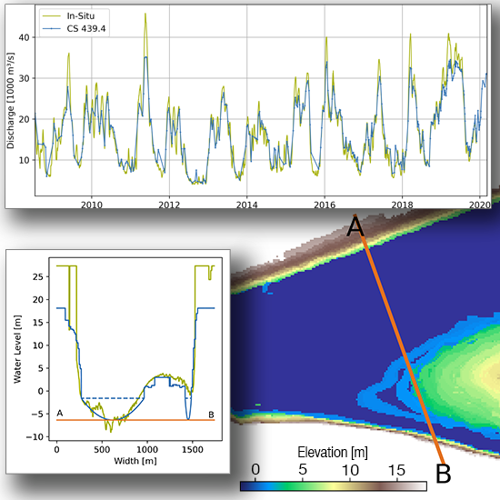
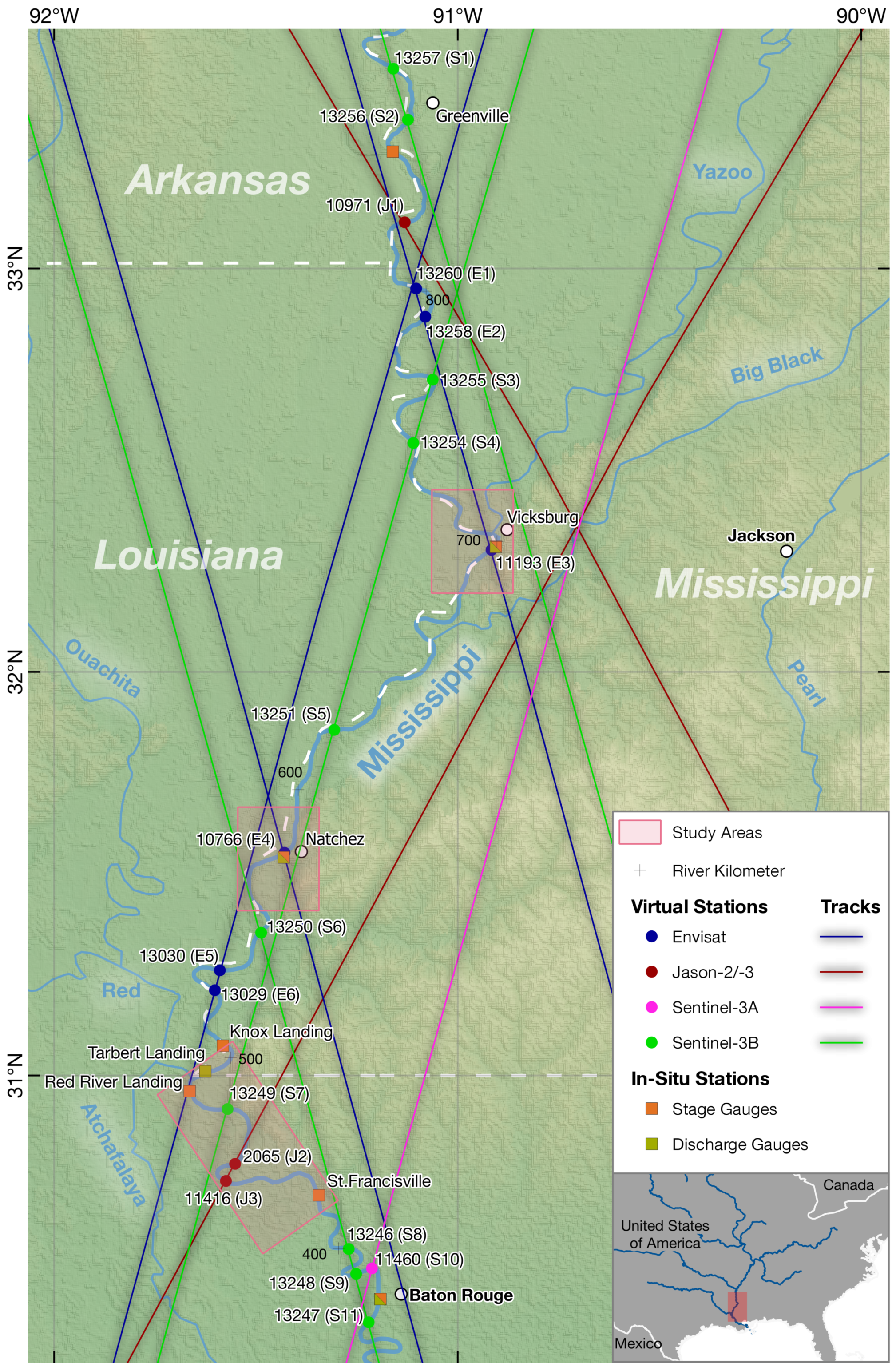
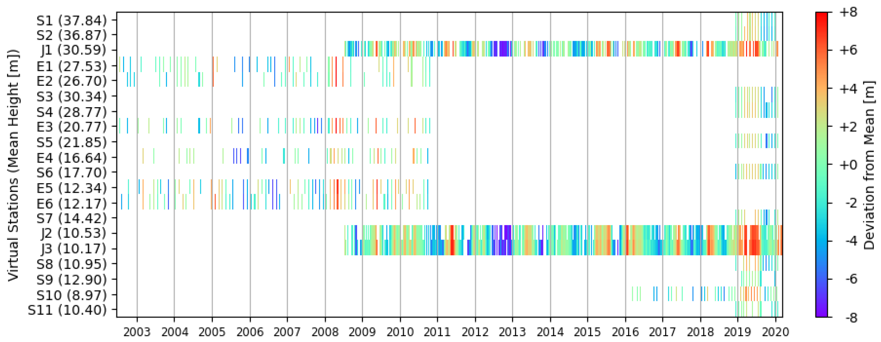
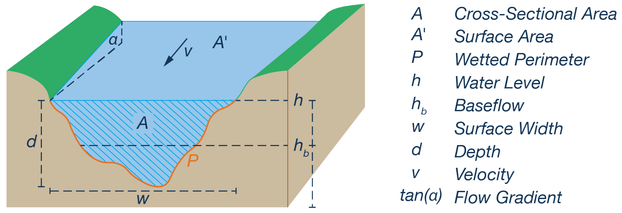
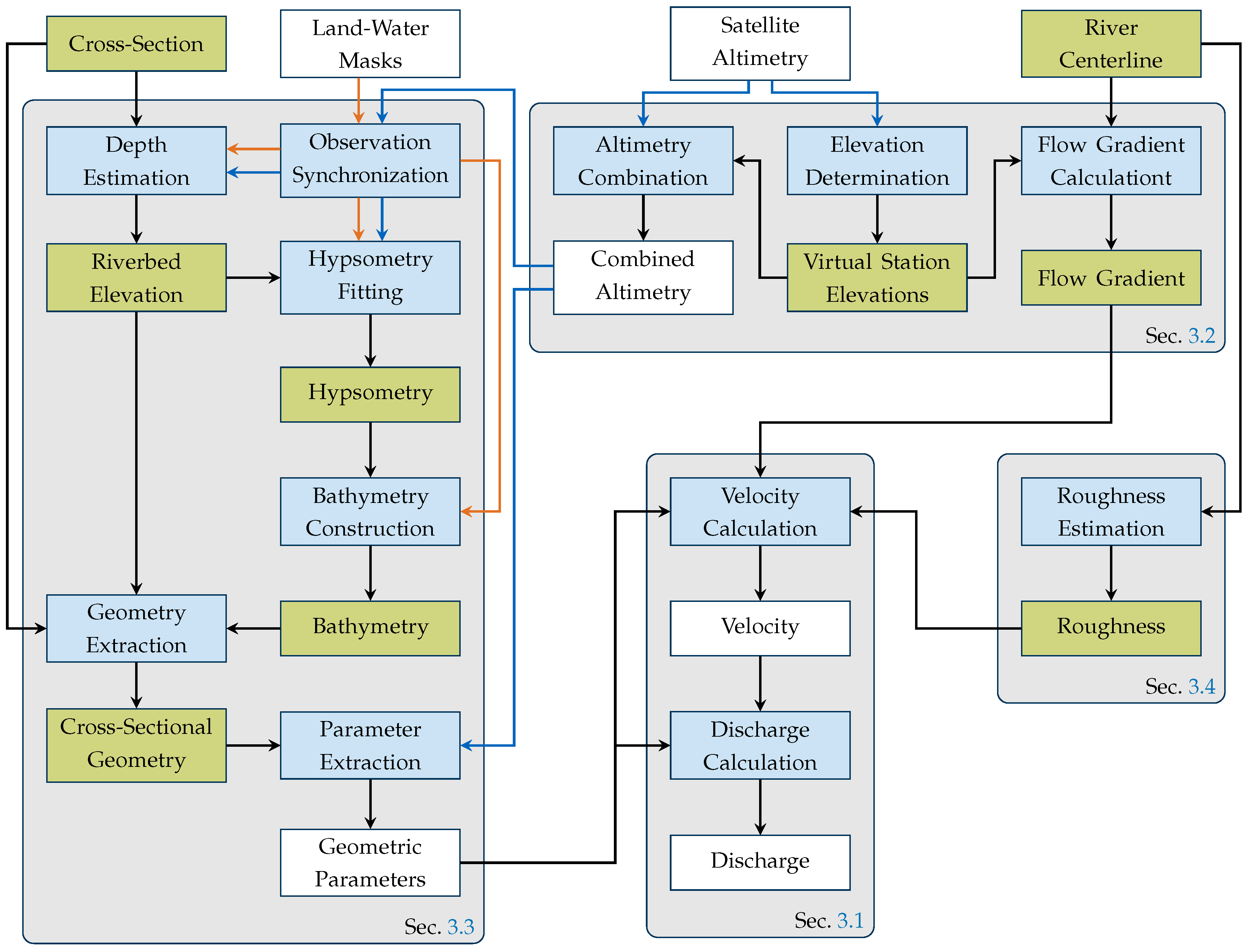
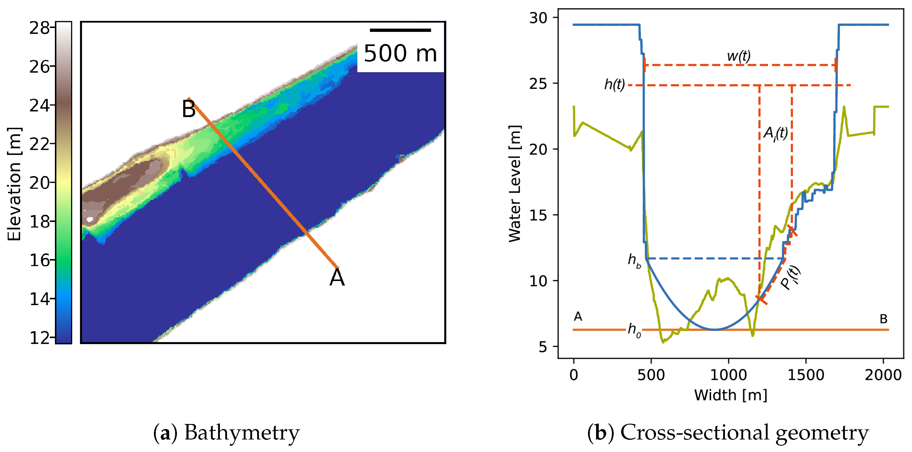
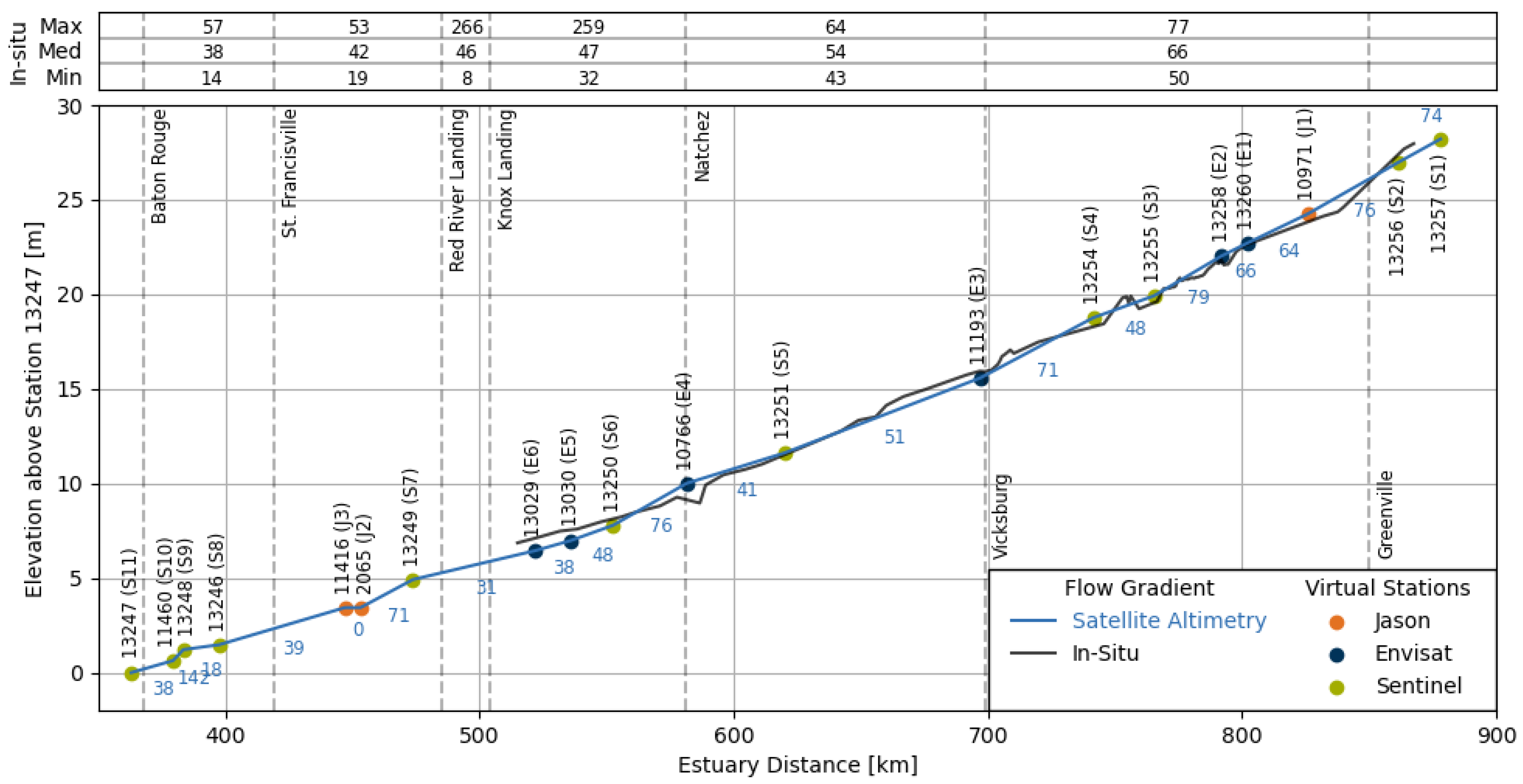
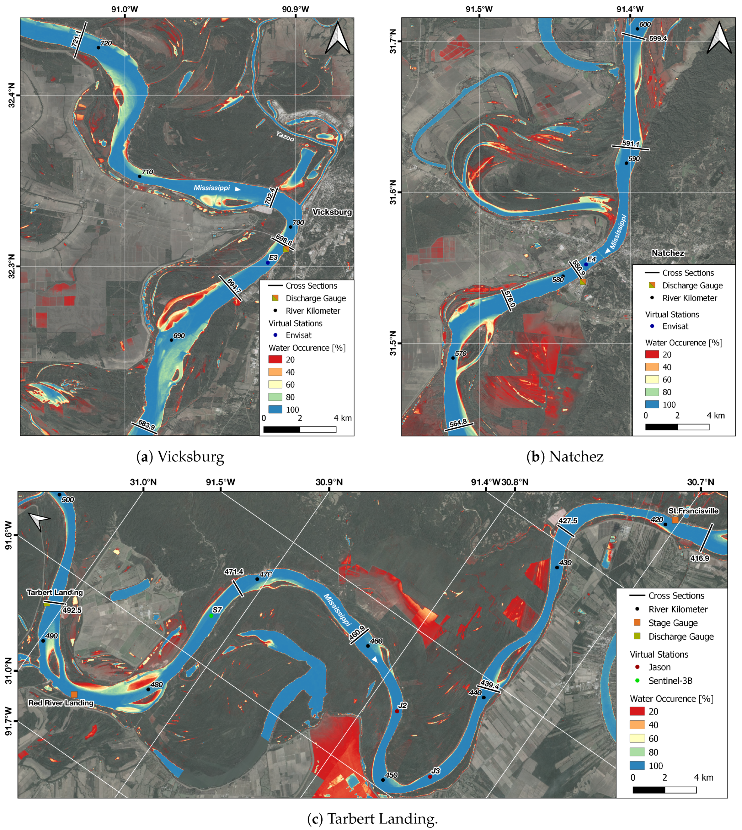
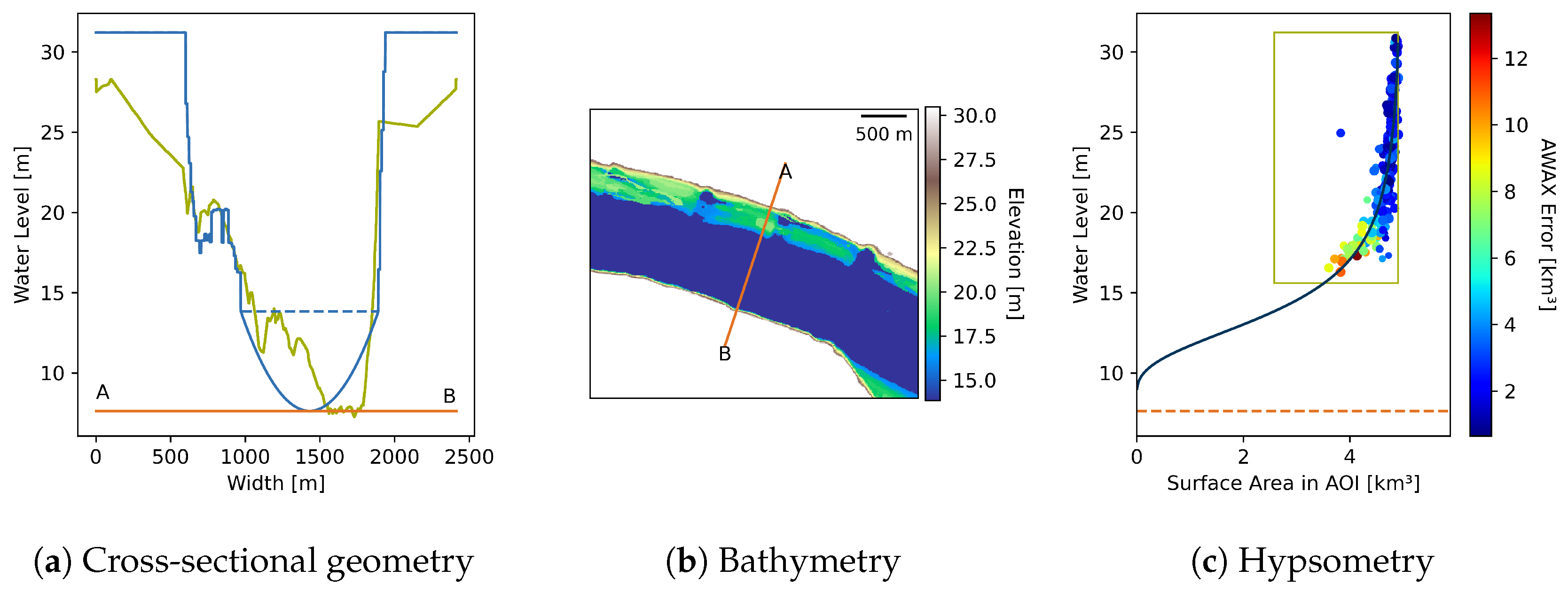
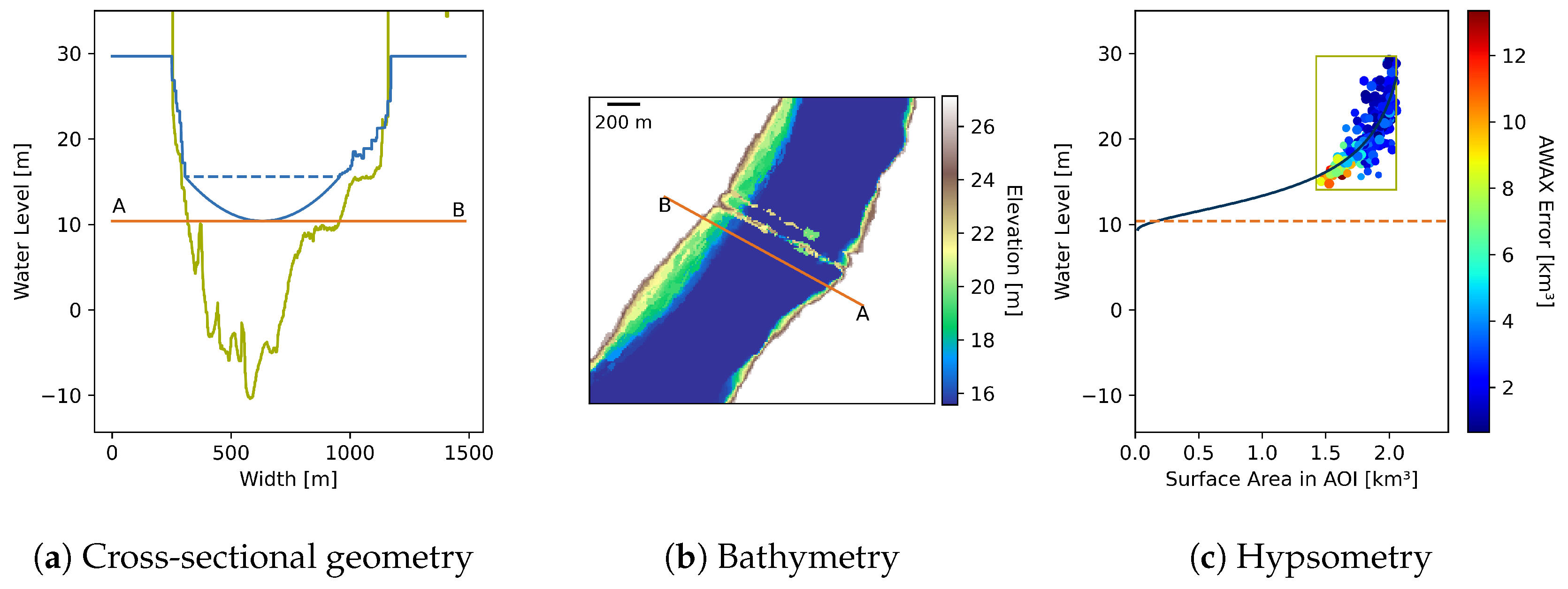
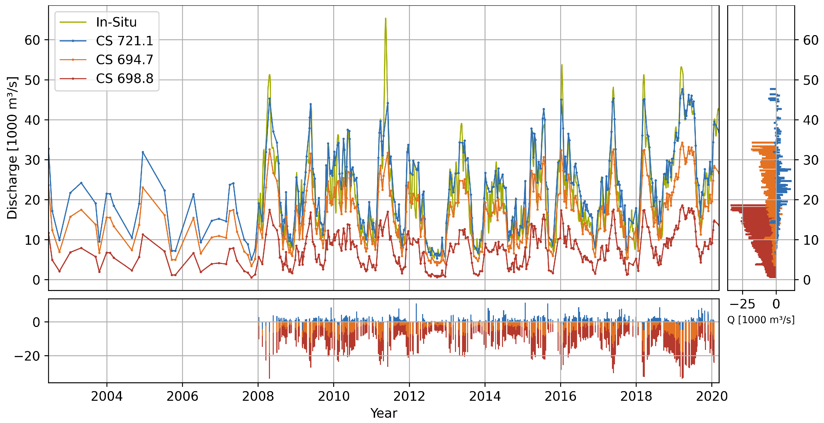
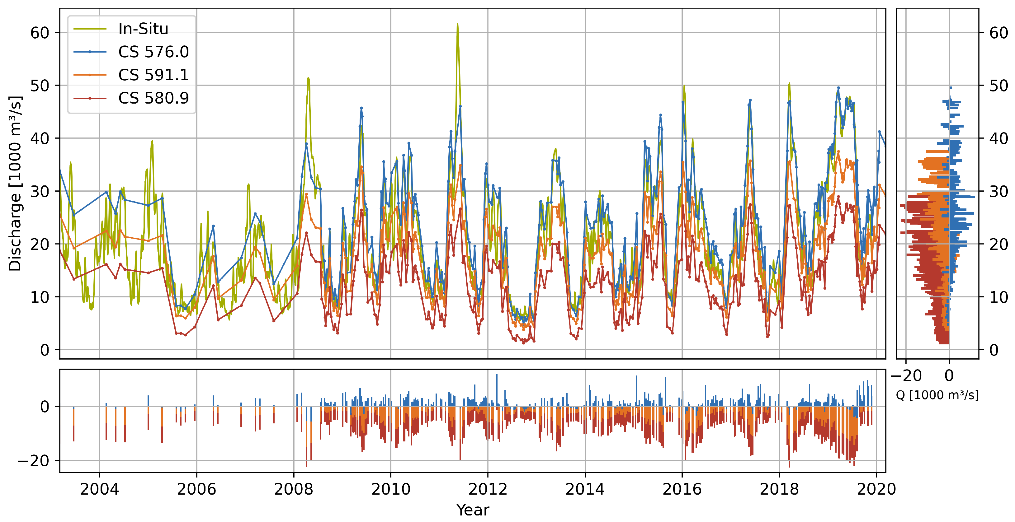
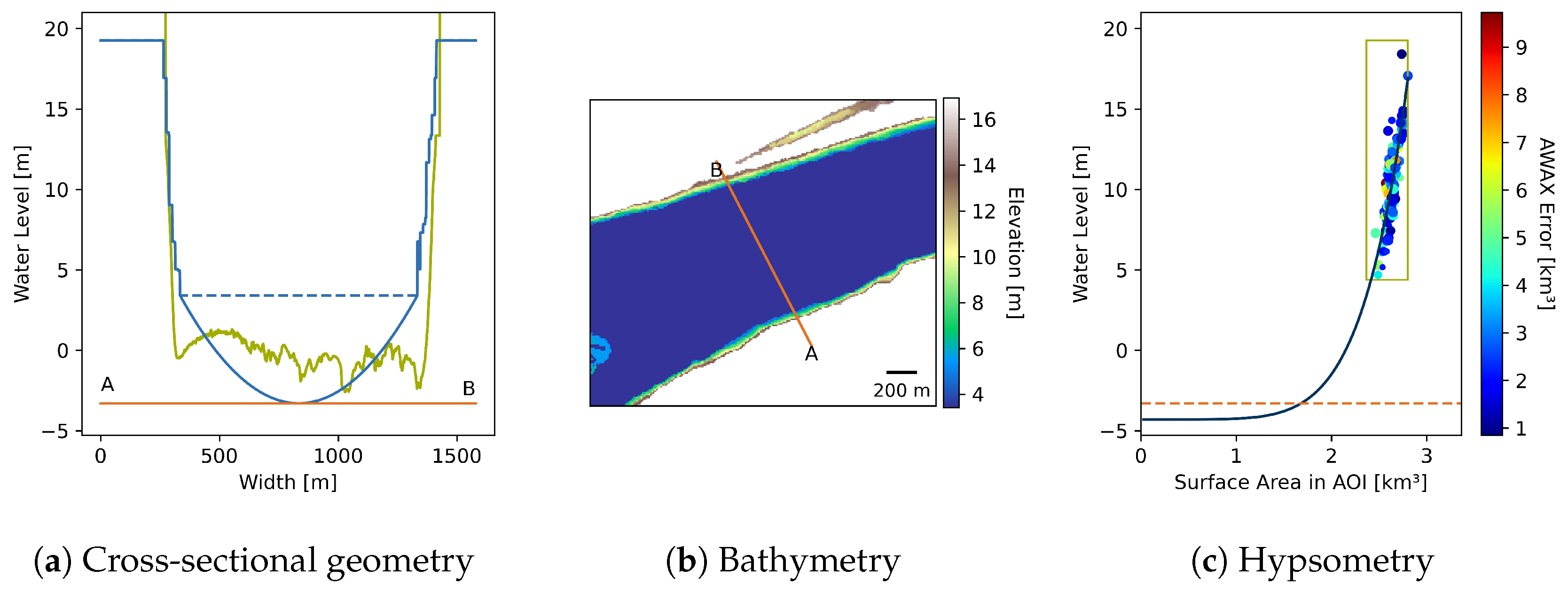
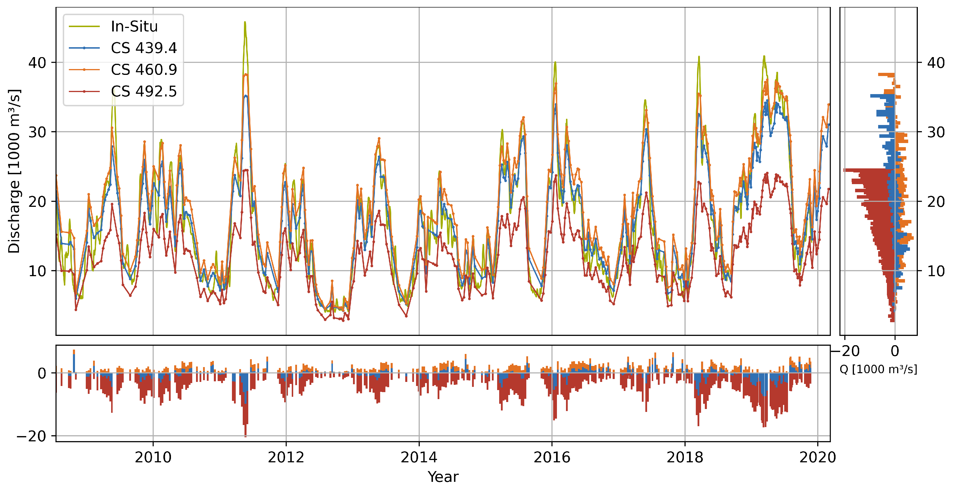
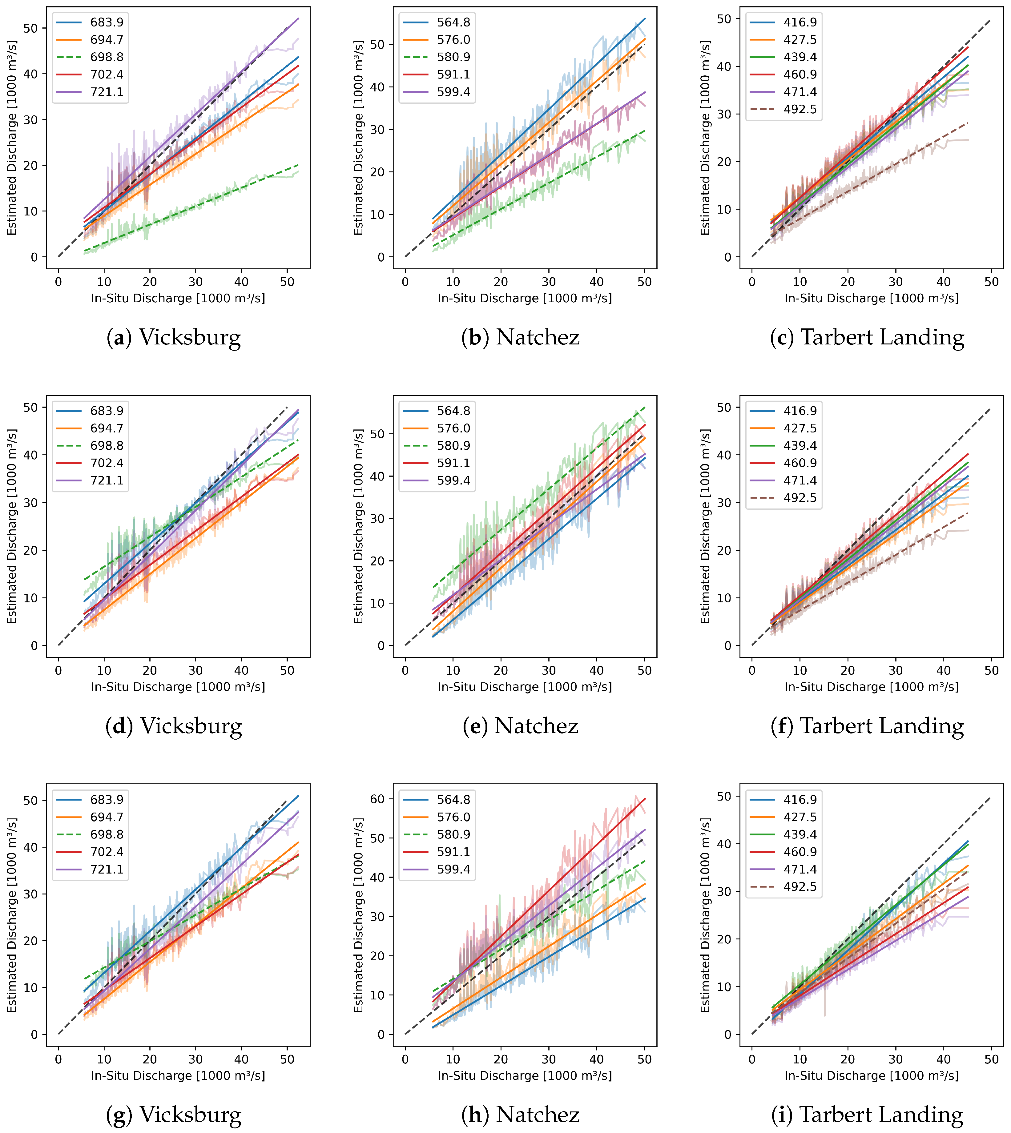
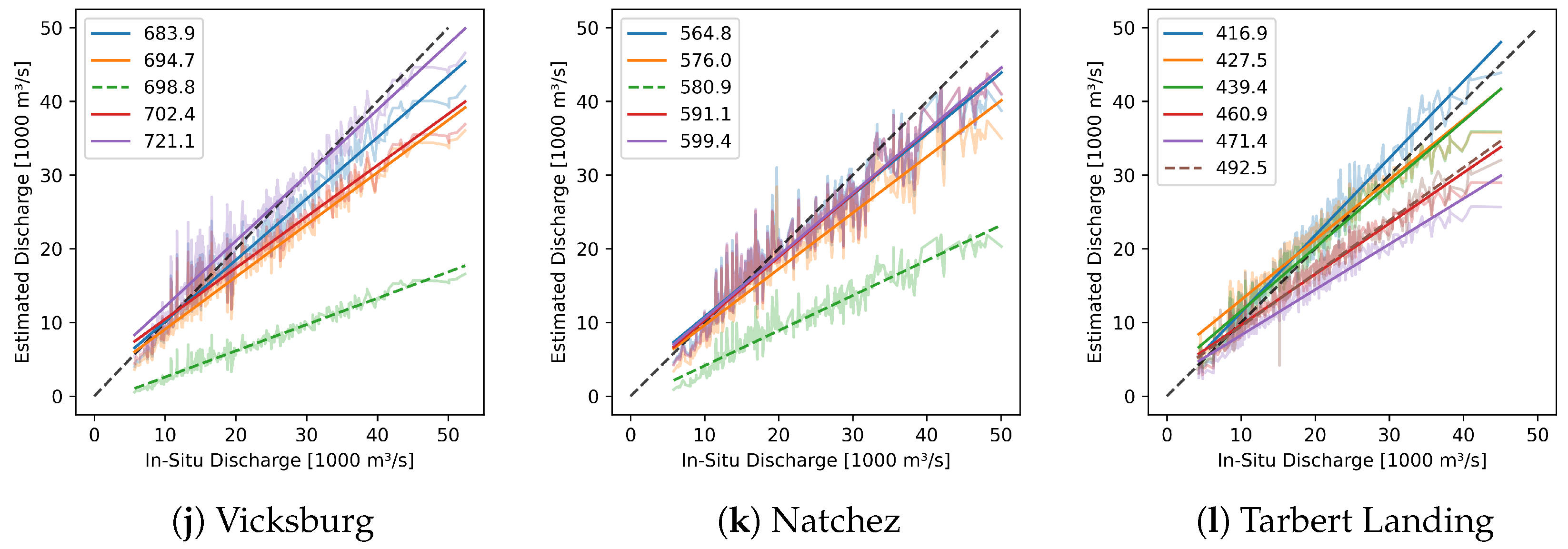
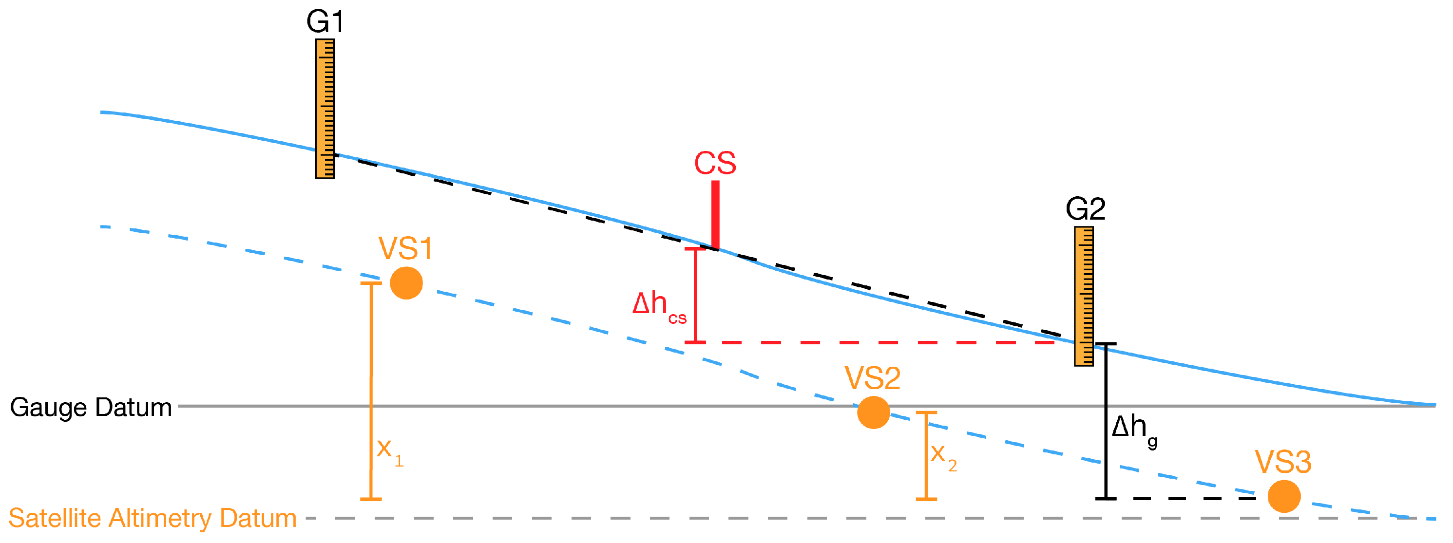
Table 1.
Satellite altimetry comparison with in situ gauges showing the distance between the two locations, the number # of synchronous observations and the respective median offset, RMSE, NRMSE and the squared Pearson correlation coefficient . The arrows indicate whether the stage (•) or combined stage and discharge (∘) gauge is located upstream (↑) or downstream (↓) of the virtual station.
| Station | Gauge | Distance | # | Offset | RMSE | NRMSE | Outliers | ||
|---|---|---|---|---|---|---|---|---|---|
| (DAHITI ID) | [km] | [m] | [%] | ||||||
| S1 (13257) | Greenville • | 28.08 | ↓ | 13 | 2.35 | 0.35 | 0.99 | 0.994 | 40 |
| S2 (13256) | 11.69 | ↓ | 14 | 1.04 | 0.11 | 0.31 | 0.999 | 40 | |
| J1 (10971) | 24.29 | ↑ | 282 | −1.85 | 0.68 | 2.11 | 0.965 | 40 | |
| E1 (13260) | 47.97 | ↑ | 42 | −3.68 | 0.73 | 2.34 | 0.951 | 40 | |
| E2 (13258) | 58.16 | ↑ | 36 | −4.37 | 0.39 | 1.24 | 0.985 | 40 | |
| S3 (13255) | Vicksburg ∘ | 66.64 | ↓ | 12 | 3.89 | 0.37 | 1.38 | 0.991 | 28 |
| S4 (13254) | 42.86 | ↓ | 14 | 2.67 | 0.53 | 2.01 | 0.969 | 28 | |
| E3 (11193) | 1.70 | ↑ | 46 | −0.17 | 1.13 | 5.44 | 0.901 | 28 | |
| S5 (13251) | Natchez ∘ | 39.08 | ↓ | 13 | 2.07 | 0.43 | 2.13 | 0.976 | 24 |
| E4 (10766) | 0.70 | ↓ | 34 | 0.19 | 0.47 | 2.86 | 0.978 | 24 | |
| S6 (13250) | 28.28 | ↑ | 14 | −1.66 | 0.51 | 2.60 | 0.976 | 24 | |
| E5 (13030) | Knox Landing • | 31.57 | ↓ | 50 | 1.18 | 0.44 | 3.98 | 0.986 | 50 |
| E6 (13029) | 17.38 | ↓ | 53 | 0.67 | 0.79 | 7.03 | 0.948 | 50 | |
| S7 (13249) | Red River Landing • | 11.40 | ↑ | 10 | −0.29 | 0.22 | 1.49 | 0.995 | 42 |
| J2 (2065) | 31.99 | ↑ | 299 | −1.50 | 0.50 | 4.23 | 0.981 | 42 | |
| J3 (11416) | St. Francisville • | 27.67 | ↓ | 347 | 1.32 | 0.49 | 5.48 | 0.979 | 9 |
| S8 (13246) | 21.77 | ↑ | 11 | −0.78 | 0.20 | 1.71 | 0.997 | 9 | |
| S9 (13248) | Baton Rouge ∘ | 15.39 | ↓ | 7 | 1.22 | 0.21 | 1.78 | 0.989 | 39 |
| S10 (11460) | 11.29 | ↓ | 29 | 0.73 | 0.14 | 1.80 | 0.998 | 39 | |
| S11 (13247) | 5.10 | ↑ | 8 | 0.07 | 0.53 | 5.08 | 0.970 | 39 |
Table 2.
Uncertainties of the adjusted virtual station (VS) elevations in millimeters.
| VS: | S1 | S2 | J1 | E1 | E2 | S3 | S4 | E3 | S5 | E4 | S6 | E5 | E6 | S7 | J2 | J3 | S8 | S9 | S10 |
|---|---|---|---|---|---|---|---|---|---|---|---|---|---|---|---|---|---|---|---|
| [mm]: | 27 | 26 | 20 | 51 | 51 | 21 | 21 | 48 | 21 | 68 | 18 | 42 | 42 | 23 | 18 | 18 | 20 | 23 | 36 |
Table 3.
Estimated Parameters (left), discharge validation results (center), and observations synchronization statistics (right) at Vicksburg using combined altimetry data from E3, J1, and S4. A and P are given as percentage and as deviation of the respective in situ data. The synchronization statistics shows the resulting number of surface area and water level observation pairs, the area-height correlation coefficient , and the average time between the synchronized observations.
| Parameters | Discharge Validation | Synchronization | |||||||||||
|---|---|---|---|---|---|---|---|---|---|---|---|---|---|
| CS | I | A | R | NSE | NRMSE | RMSE | Pairs | ||||||
| [] | [%] | [%] | [m] | [m/s] | [%] | [m/s] | [Days] | ||||||
| 683.9 | 51 | 50.00 | 92.72 | 109.31 | 2.70 | −2130.80 | 0.873 | 17.34 | 3827 | 0.974 | 239 | 0.681 | 5.00 |
| 694.7 | 51 | 43.48 | 98.14 | 104.40 | 0.97 | −4321.02 | 0.658 | 28.43 | 6275 | 0.976 | 239 | 0.704 | 5.00 |
| 698.8 | 71 | 38.46 | 60.72 | 60.96 | 20.78 | −13457.17 | −1.112 | 70.69 | 15604 | 0.960 | 239 | 0.634 | 5.00 |
| 702.4 | 71 | 38.46 | 102.47 | 105.63 | 3.84 | −1938.45 | 0.844 | 19.24 | 4246 | 0.978 | 239 | 0.748 | 5.00 |
| 721.1 | 71 | 50.00 | 97.38 | 161.45 | 0.37 | 1471.94 | 0.929 | 12.96 | 2861 | 0.975 | 239 | 0.720 | 5.00 |
Table 4.
Estimated Parameters (left), discharge validation results (center), and observations synchronization statistics (right) at Natchez using combined altimetry data from E4, J1, S5, and S6. For details see Table 3.
Table 4.
Estimated Parameters (left), discharge validation results (center), and observations synchronization statistics (right) at Natchez using combined altimetry data from E4, J1, S5, and S6. For details see Table 3.
| Parameters | Discharge Validation | Synchronization | |||||||||||
|---|---|---|---|---|---|---|---|---|---|---|---|---|---|
| CS | I | A | R | NSE | NRMSE | RMSE | Pairs | ||||||
| [] | [%] | [%] | [m] | [m/s] | [%] | [m/s] | [Days] | ||||||
| 564.8 | 76 | 50.00 | 125.53 | 140.19 | −2.43 | 4094.80 | 0.785 | 21.92 | 5059 | 0.963 | 232 | 0.829 | 5.14 |
| 576.0 | 76 | 50.00 | 99.43 | 118.78 | −0.86 | 1625.15 | 0.921 | 13.26 | 3060 | 0.966 | 232 | 0.572 | 5.14 |
| 580.9 | 76 | 50.00 | 59.14 | 83.75 | 11.90 | −9632.32 | −0.002 | 47.27 | 10912 | 0.956 | 232 | 0.714 | 5.14 |
| 591.1 | 41 | 50.00 | 76.13 | 111.05 | 1.54 | −3714.84 | 0.745 | 23.83 | 5500 | 0.966 | 232 | 0.715 | 5.14 |
| 599.4 | 41 | 50.00 | 87.92 | 104.37 | 7.10 | −3516.56 | 0.754 | 23.42 | 5405 | 0.967 | 232 | 0.655 | 5.14 |
Table 5.
Estimated Parameters (left), discharge validation results (center), and observations synchronization statistics (right) at Tarbert Landing using combined altimetry data from J2, S7, S9, and S10. For details see Table 3.
Table 5.
Estimated Parameters (left), discharge validation results (center), and observations synchronization statistics (right) at Tarbert Landing using combined altimetry data from J2, S7, S9, and S10. For details see Table 3.
| Parameters | Discharge Validation | Synchronization | |||||||||||
|---|---|---|---|---|---|---|---|---|---|---|---|---|---|
| CS | I | A | R | NSE | NRMSE | RMSE | Pairs | ||||||
| [] | [%] | [%] | [m] | [m/s] | [%] | [m/s] | [Days] | ||||||
| 416.9 | 39 | 50.00 | 115.52 | 117.83 | 6.41 | 1191.17 | 0.933 | 12.12 | 2226 | 0.981 | 148 | 0.899 | 4.12 |
| 427.5 | 39 | 43.48 | 116.25 | 117.48 | −0.71 | 1188.82 | 0.924 | 12.97 | 2381 | 0.982 | 148 | 0.847 | 4.12 |
| 439.4 | 39 | 50.00 | 103.66 | 100.79 | 2.69 | −109.32 | 0.946 | 10.95 | 2011 | 0.978 | 148 | 0.818 | 4.12 |
| 460.9 | 72 | 43.48 | 107.07 | 109.58 | 2.58 | 1541.46 | 0.925 | 12.86 | 2361 | 0.980 | 147 | 0.712 | 4.00 |
| 471.4 | 72 | 43.48 | 102.30 | 112.37 | 3.66 | −555.25 | 0.926 | 12.76 | 2344 | 0.979 | 147 | 0.794 | 4.00 |
| 492.5 | 31 | 43.48 | 99.76 | 101.60 | −0.70 | −4914.37 | 0.389 | 36.73 | 6745 | 0.980 | 136 | 0.582 | 4.38 |
Table 6.
Errors of the discharge estimation using estimated parameters and respective increase (+) or decrease (−) using in situ substitutions per CS. The right column shows the significant parameter causing the largest error.
Table 6.
Errors of the discharge estimation using estimated parameters and respective increase (+) or decrease (−) using in situ substitutions per CS. The right column shows the significant parameter causing the largest error.
| CS | Estimated | Substitute | Significant | ||
|---|---|---|---|---|---|
| I | A and P | I, A, and P | Parameter | ||
| NRMSE[%] | NRMSE[%] | NRMSE[%] | NRMSE[%] | ||
| 721.1 | 12.96 | −1.02 | −2.13 | +0.65 | Roughness |
| 702.4 | 19.24 | +3.19 | +3.97 | +7.24 | Roughness |
| 698.8 | 70.69 | +5.03 | −49.11 | −47.87 | Bathymetry |
| 694.7 | 28.43 | −2.72 | +0.30 | −2.31 | Roughness |
| 683.9 | 17.34 | −2.58 | −4.90 | −3.79 | Roughness |
| 599.4 | 23.42 | −9.76 | −11.25 | −6.09 | All |
| 591.1 | 23.83 | −9.96 | −10.69 | +4.24 | Roughness |
| 580.9 | 47.27 | +13.40 | −14.32 | −30.78 | Bathymetry |
| 576.0 | 13.26 | +8.42 | −0.27 | +16.95 | Roughness |
| 564.8 | 21.92 | −6.60 | +0.29 | +17.76 | Roughness |
| 492.5 | 36.73 | −14.84 | +2.46 | −12.23 | Gradient |
| 471.4 | 12.76 | +19.92 | +3.84 | +24.11 | Roughness |
| 460.9 | 12.86 | +9.80 | -1.51 | +18.72 | Roughness |
| 439.4 | 10.95 | −0.47 | +3.49 | +1.03 | Roughness |
| 427.5 | 12.97 | +1.27 | +10.77 | +7.67 | Roughness |
| 416.9 | 12.12 | +1.47 | +8.50 | +3.06 | Roughness |
© 2020 by the authors. Licensee MDPI, Basel, Switzerland. This article is an open access article distributed under the terms and conditions of the Creative Commons Attribution (CC BY) license (http://creativecommons.org/licenses/by/4.0/).
Share and Cite
MDPI and ACS Style
Scherer, D.; Schwatke, C.; Dettmering, D.; Seitz, F. Long-Term Discharge Estimation for the Lower Mississippi River Using Satellite Altimetry and Remote Sensing Images. Remote Sens. 2020, 12, 2693. https://doi.org/10.3390/rs12172693
AMA Style
Scherer D, Schwatke C, Dettmering D, Seitz F. Long-Term Discharge Estimation for the Lower Mississippi River Using Satellite Altimetry and Remote Sensing Images. Remote Sensing. 2020; 12(17):2693. https://doi.org/10.3390/rs12172693
Chicago/Turabian StyleScherer, Daniel, Christian Schwatke, Denise Dettmering, and Florian Seitz. 2020. "Long-Term Discharge Estimation for the Lower Mississippi River Using Satellite Altimetry and Remote Sensing Images" Remote Sensing 12, no. 17: 2693. https://doi.org/10.3390/rs12172693
Note that from the first issue of 2016, this journal uses article numbers instead of page numbers. See further details here.