Using UAV Collected RGB and Multispectral Images to Evaluate Winter Wheat Performance across a Site Characterized by Century-Old Biochar Patches in Belgium

 , , , and
Abstract
:1. Introduction
2. Materials and Methods
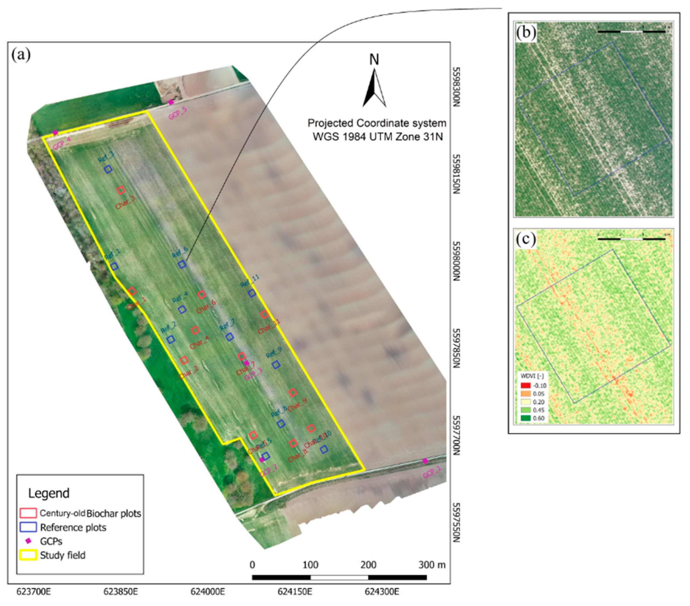
2.1. Site Description and Data Acquisition
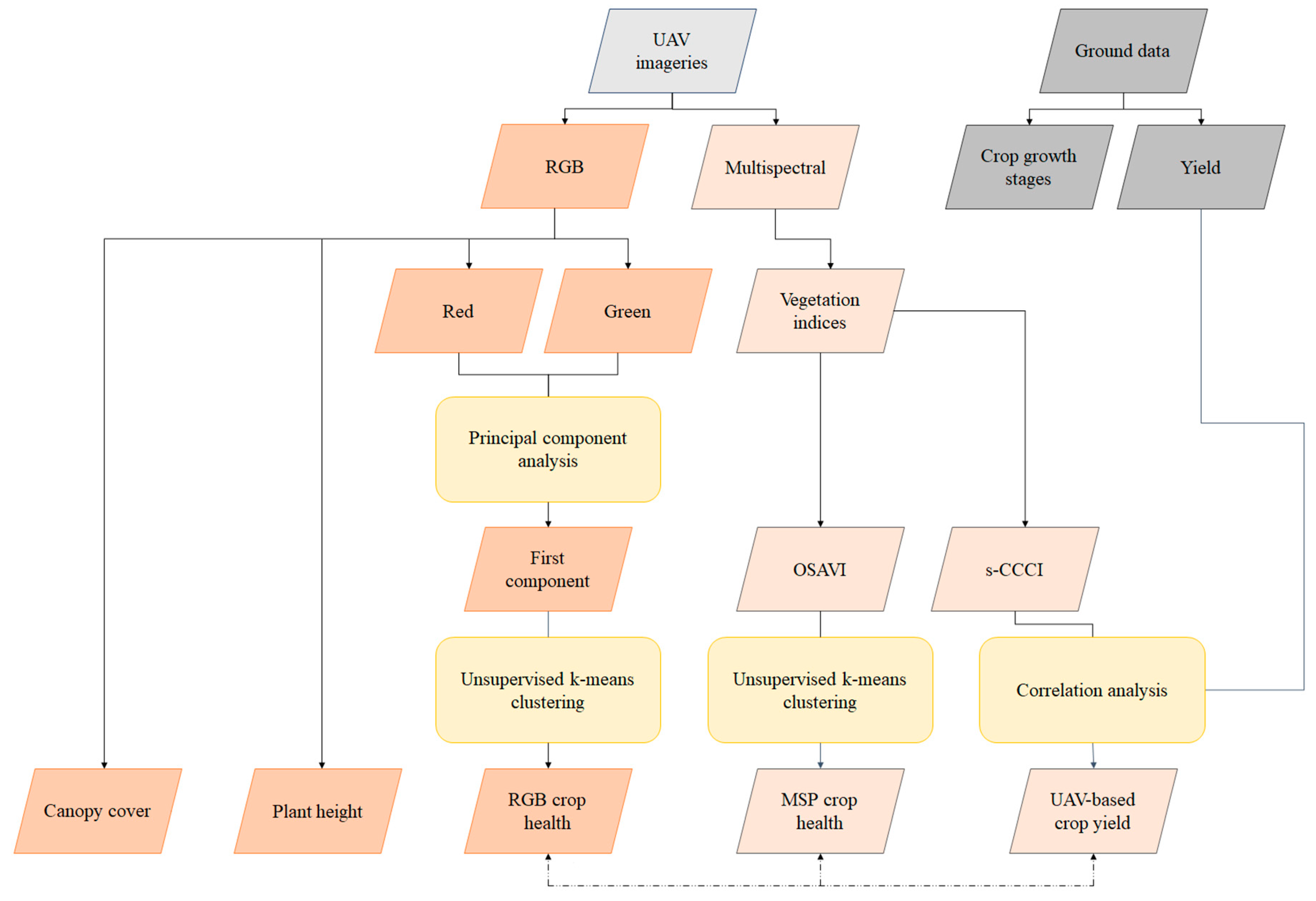
2.2. UAV-Based Crop Monitoring
2.3. Statistical Analysis
3. Results and Discussion
3.1. UAV-Based Crop Assessment
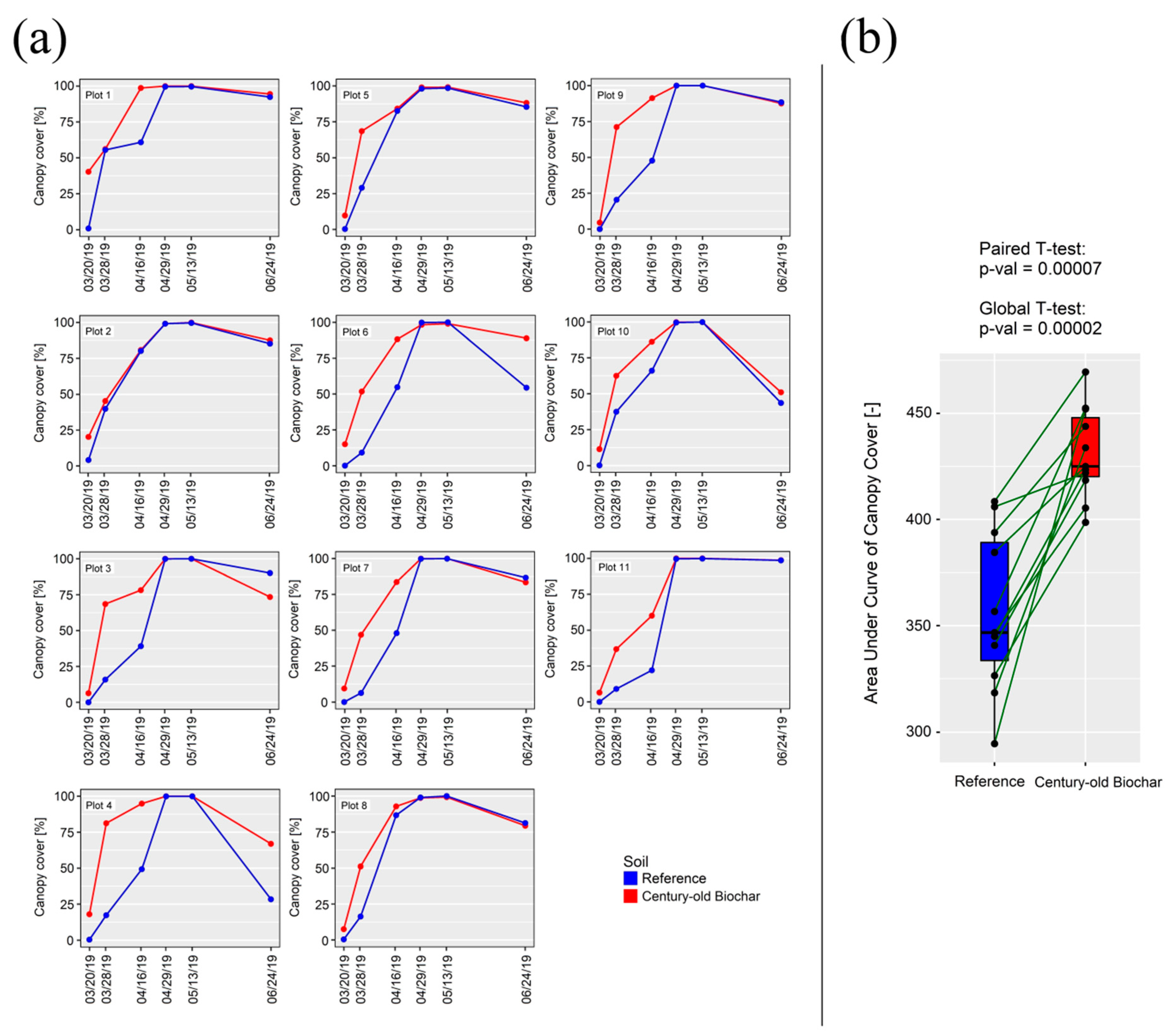
3.1.1. Canopy Cover
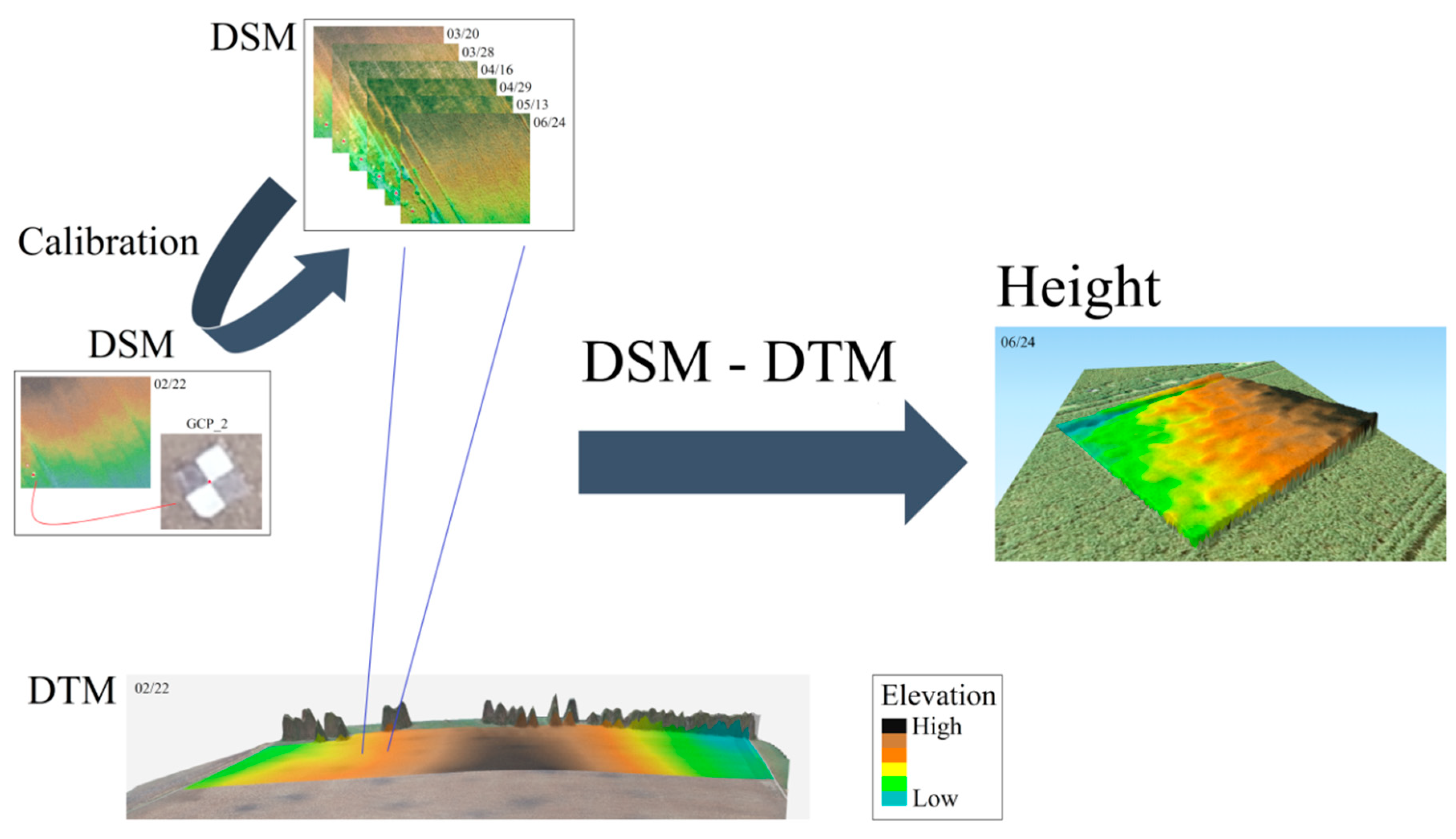
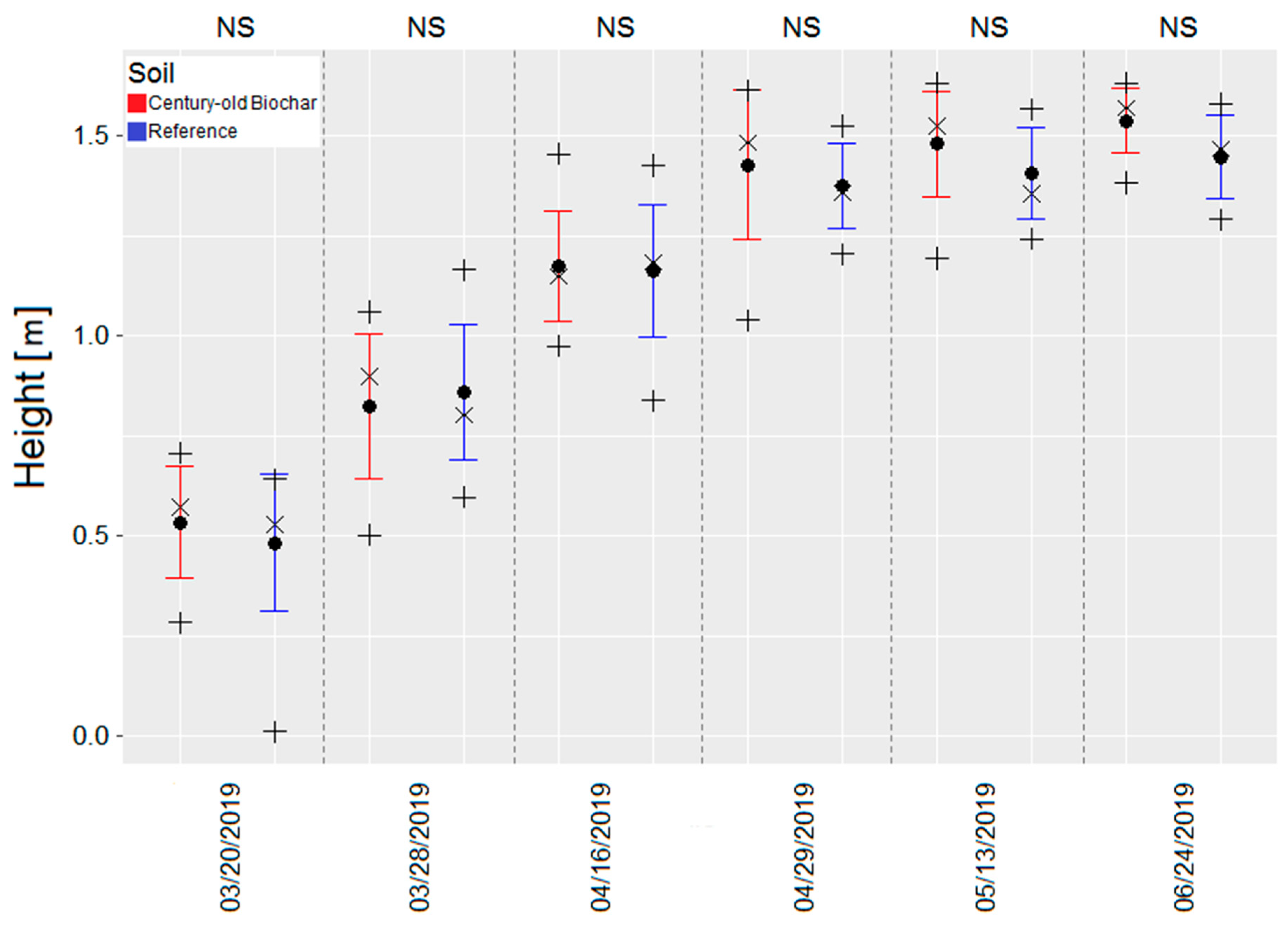
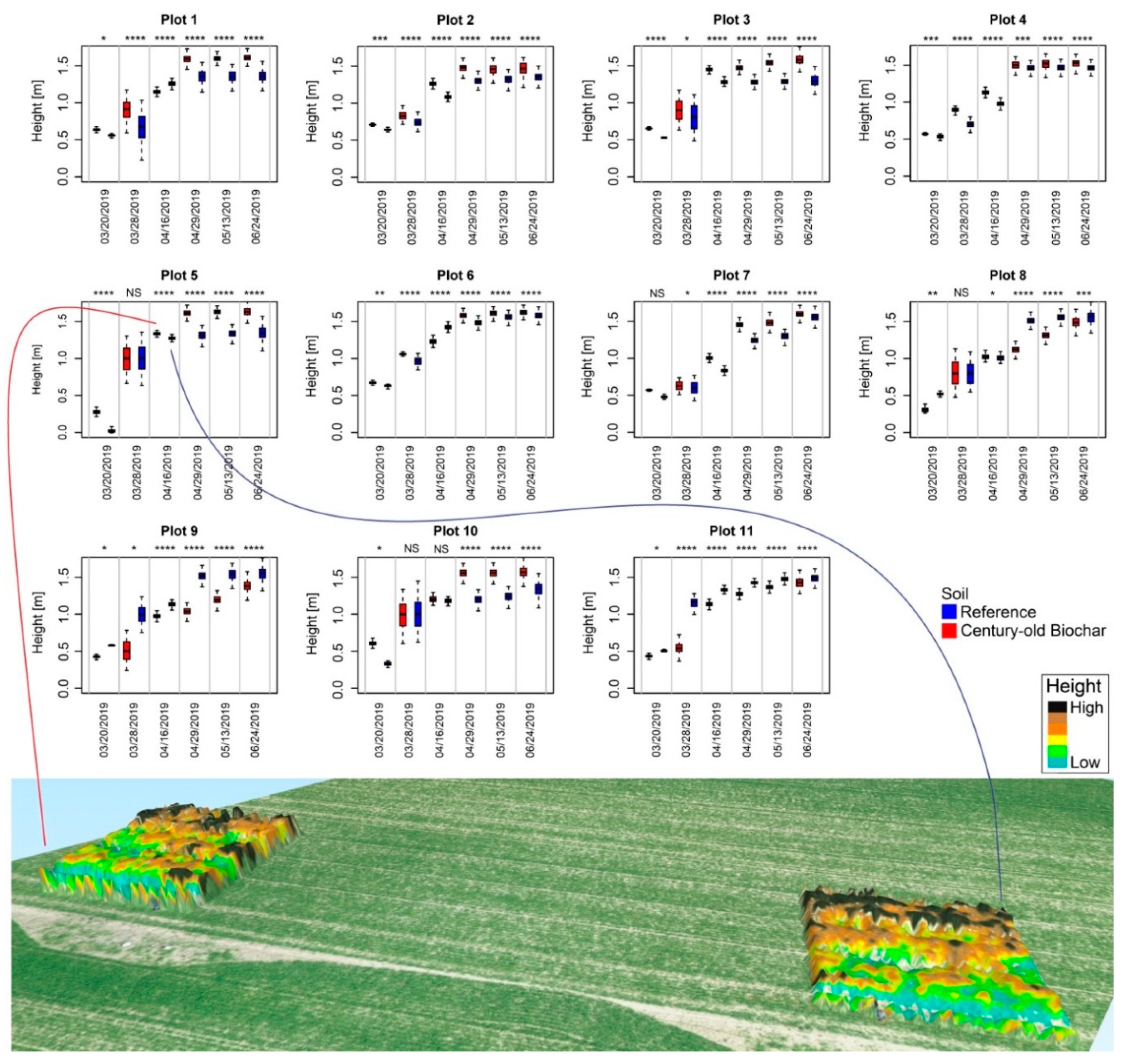
3.1.2. Plant Height
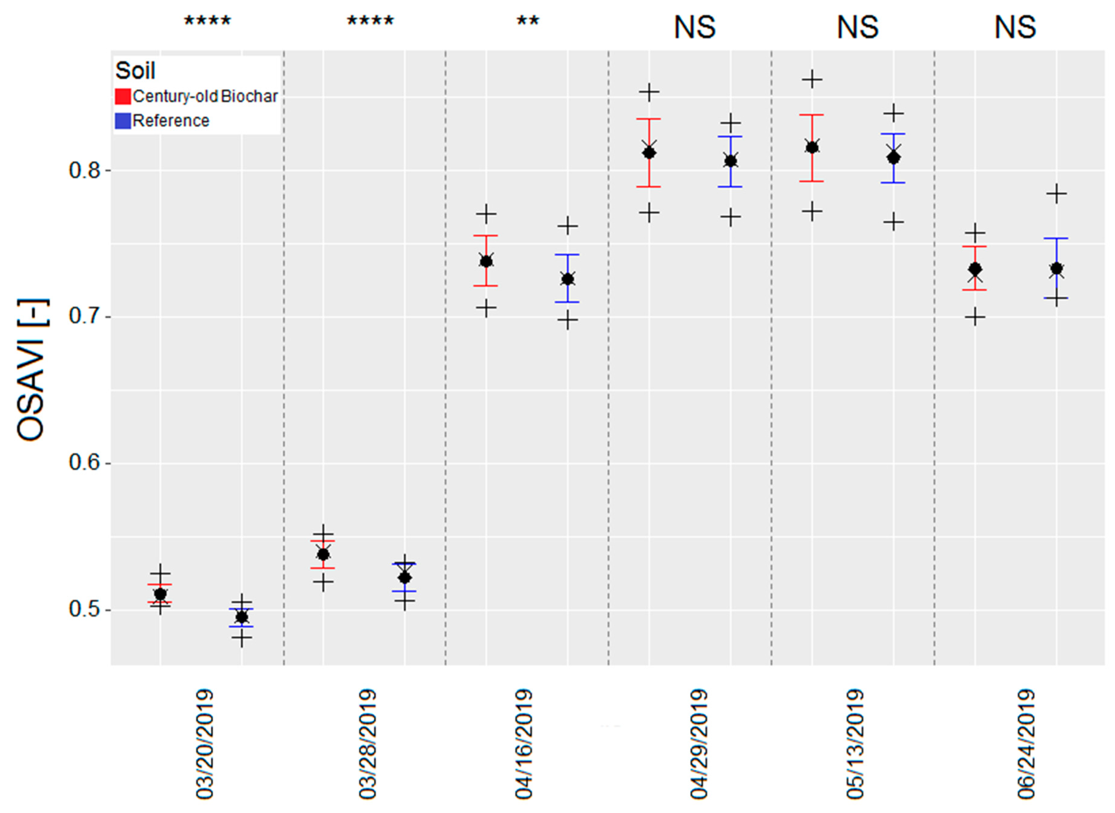
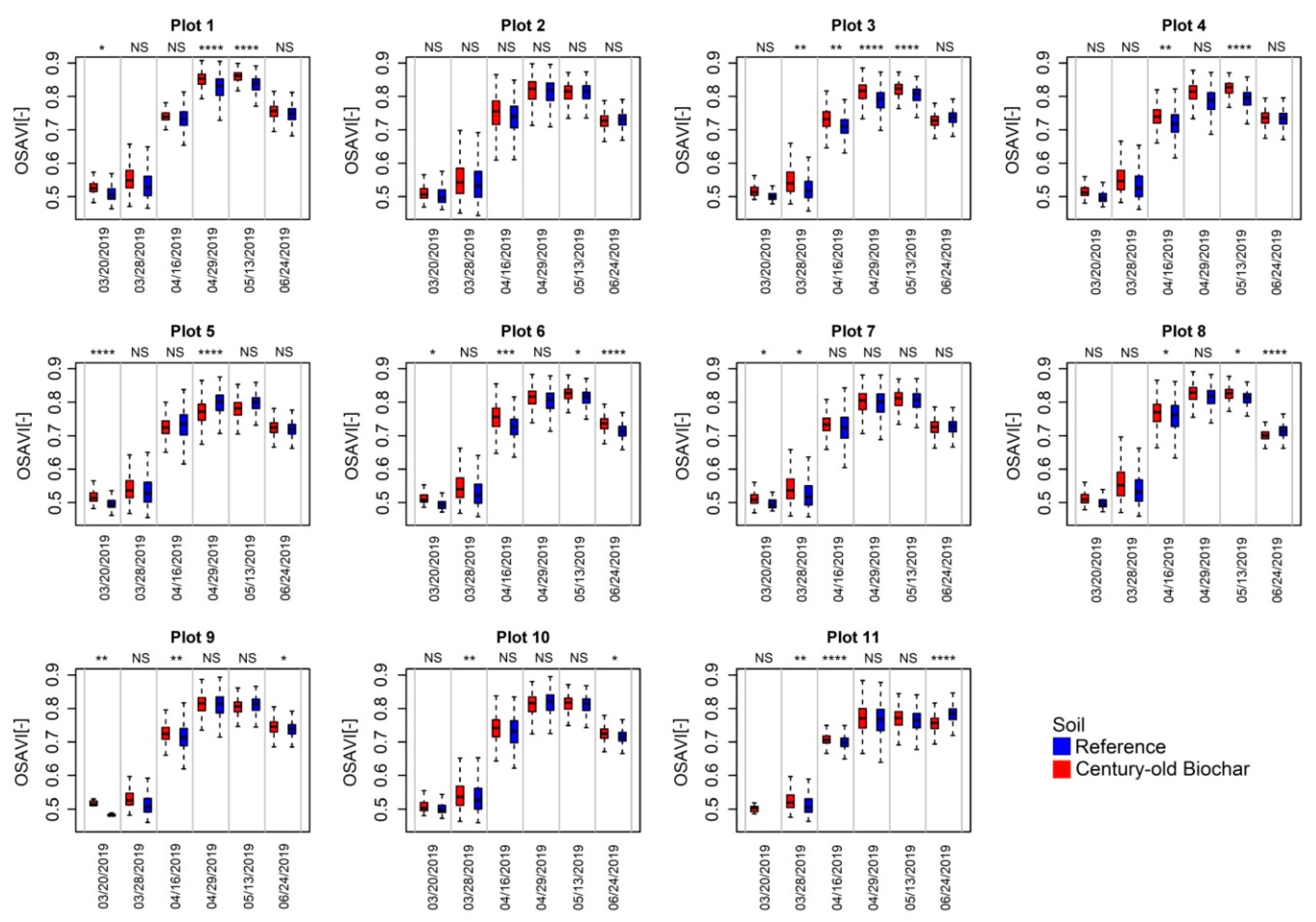
3.1.3. Vegetation Indices
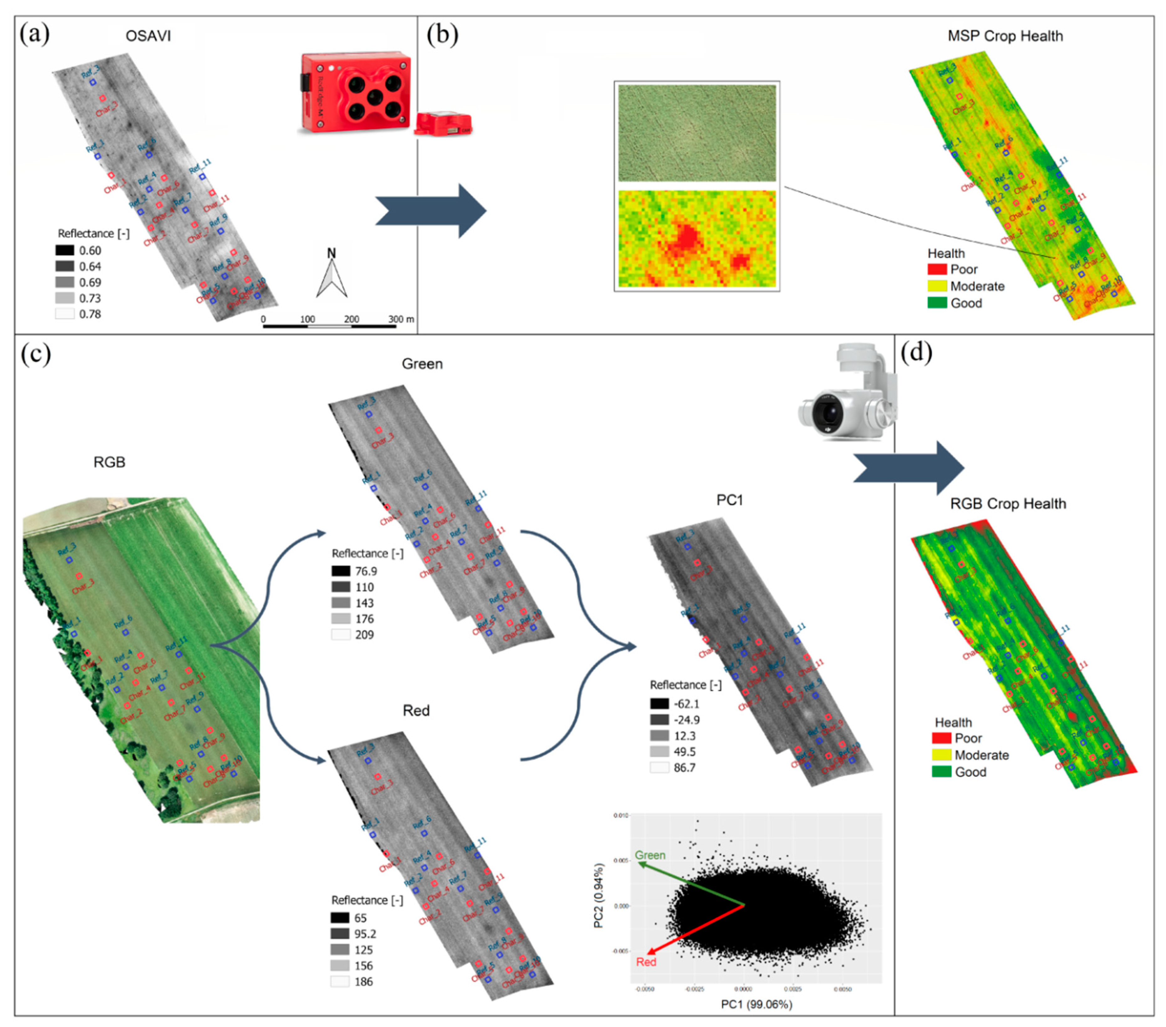
3.1.4. Crop Health
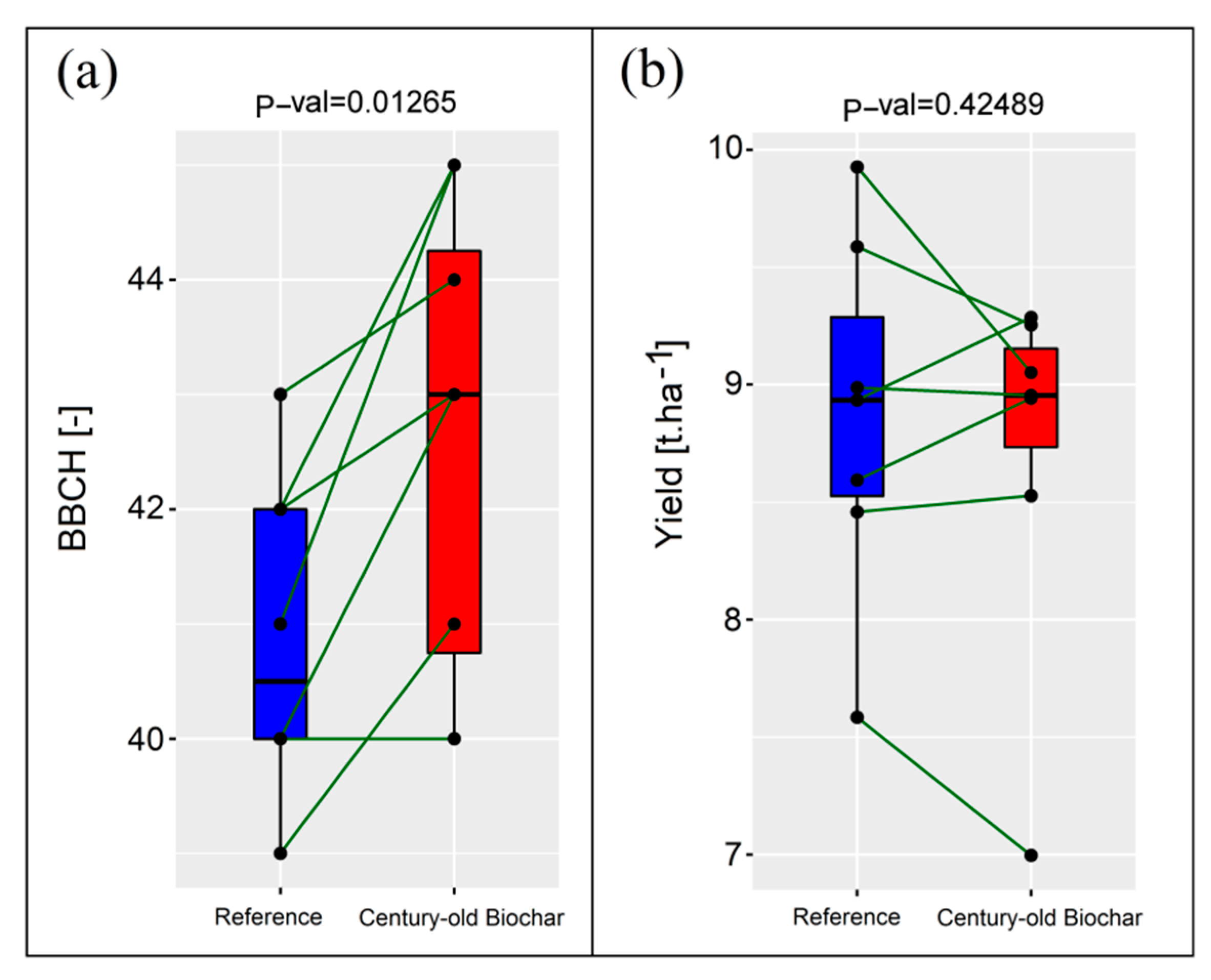
3.2. Ground-Based Crop Evaluation and Harvested Crop Yield
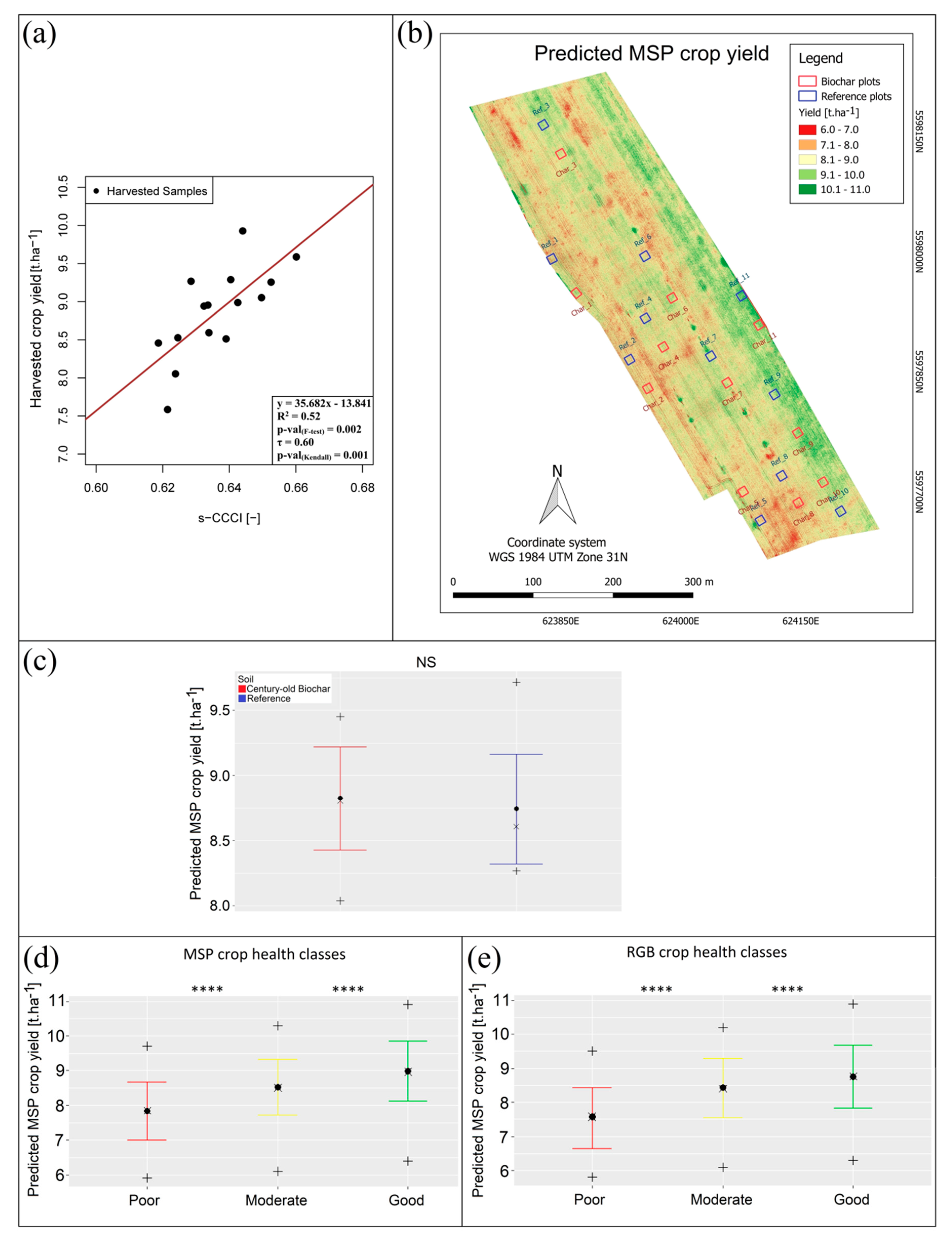
3.3. UAV-Based Yield Map Generation
4. Conclusions
Author Contributions
Funding
Acknowledgments
Conflicts of Interest
References
- Malghani, S.; Gleixner, G.; Trumbore, S.E. Chars produced by slow pyrolysis and hydrothermal carbonization vary in carbon sequestration potential and greenhouse gases emissions. Soil Biol. Biochem. 2013, 62, 137–146. [Google Scholar] [CrossRef] [Green Version]
- Trupiano, D.; Cocozza, C.; Baronti, S.; Amendola, C.; Vaccari, F.P.; Lustrato, G.; Di Lonardo, S.; Fantasma, F.; Tognetti, R.; Scippa, G.S. The effects of biochar and its combination with compost on lettuce (Lactuca sativa L.) growth, soil properties, and soil microbial activity and abundance. Int. J. Agron. 2017, 2017, 3158207. [Google Scholar] [CrossRef] [Green Version]
- Yamato, M.; Okimori, Y.; Wibowo, I.F.; Anshori, S.; Ogawa, M. Effects of the application of charred bark of Acacia mangium on the yield of maize, cowpea and peanut, and soil chemical properties in South Sumatra, Indonesia. Soil Sci. Plant Nutr. 2006, 52, 489–495. [Google Scholar] [CrossRef]
- Montanarella, L.; Lugato, E. The Application of Biochar in the EU: Challenges and Opportunities. Agronomy 2013, 3, 462–473. [Google Scholar] [CrossRef] [Green Version]
- Stewart, C.E.; Zheng, J.; Botte, J.; Cotrufo, M.F. Co-generated fast pyrolysis biochar mitigates green-house gas emissions and increases carbon sequestration in temperate soils. Gcb Bioenergy 2013, 5, 153–164. [Google Scholar] [CrossRef]
- Kerré, B.; Willaert, B.; Cornelis, Y.; Smolders, E. Long-term presence of charcoal increases maize yield in Belgium due to increased soil water availability. Eur. J. Agron. 2017, 91, 10–15. [Google Scholar] [CrossRef]
- Lehmann, J.; Da Silva, J.P.; Steiner, C.; Nehls, T.; Zech, W.; Glaser, B. Nutrient availability and leaching in an archaeological Anthrosol and a Ferralsol of the Central Amazon basin: Fertilizer, manure and charcoal amendments. Plant Soil 2003, 249, 343–357. [Google Scholar] [CrossRef]
- Biederman, L.A.; Stanley Harpole, W. Biochar and its effects on plant productivity and nutrient cycling: A meta-analysis. Gcb Bioenergy 2013, 5, 202–214. [Google Scholar] [CrossRef]
- Glaser, B.; Lehmann, J.; Zech, W. Ameliorating physical and chemical properties of highly weathered soils in the tropics with charcoal—A review. Biol. Fertil. Soils 2002, 35, 219–230. [Google Scholar] [CrossRef]
- Jeffery, S.; Meinders, M.B.J.; Stoof, C.R.; Bezemer, T.M.; van de Voorde, T.F.J.; Mommer, L.; van Groenigen, J.W. Biochar application does not improve the soil hydrological function of a sandy soil. Geoderma 2015, 251–252, 47–54. [Google Scholar] [CrossRef]
- De la Rosa, J.M.; Paneque, M.; Miller, A.Z.; Knicker, H. Relating physical and chemical properties of four different biochars and their application rate to biomass production of Lolium perenne on a Calcic Cambisol during a pot experiment of 79 days. Sci. Total Environ. 2014, 499, 175–184. [Google Scholar] [CrossRef] [PubMed] [Green Version]
- Gray, M.; Johnson, M.G.; Dragila, M.I.; Kleber, M. Water uptake in biochars: The roles of porosity and hydrophobicity. Biomass Bioenergy 2014, 61, 196–205. [Google Scholar] [CrossRef]
- Hardie, M.; Clothier, B.; Bound, S.; Oliver, G.; Close, D. Does biochar influence soil physical properties and soil water availability? Plant Soil 2014, 376, 347–361. [Google Scholar] [CrossRef]
- Liu, X.; Zhang, A.; Ji, C.; Joseph, S.; Bian, R.; Li, L.; Pan, G.; Paz-Ferreiro, J. Biochar’s effect on crop productivity and the dependence on experimental conditions-a meta-analysis of literature data. Plant Soil 2013, 373, 583–594. [Google Scholar] [CrossRef]
- Glaser, B.; Wiedner, K.; Seelig, S.; Schmidt, H.P.; Gerber, H. Biochar organic fertilizers from natural resources as substitute for mineral fertilizers. Agron. Sustain. Dev. 2015, 35, 667–678. [Google Scholar] [CrossRef] [Green Version]
- Lehmann, J.; Rillig, M.C.; Thies, J.; Masiello, C.A.; Hockaday, W.C.; Crowley, D. Biochar effects on soil biota—A review. Soil Biol. Biochem. 2011, 43, 1812–1836. [Google Scholar] [CrossRef]
- Major, J.; Rondon, M.; Molina, D.; Riha, S.J.; Lehmann, J. Maize yield and nutrition during 4 years after biochar application to a Colombian savanna oxisol. Plant Soil 2010, 333, 117–128. [Google Scholar] [CrossRef]
- Liang, B.; Lehmann, J.; Solomon, D.; Kinyangi, J.; Grossman, J.; O’Neill, B.; Skjemstad, J.O.; Thies, J.; Luizão, F.J.; Petersen, J.; et al. Black Carbon Increases Cation Exchange Capacity in Soils. Soil Sci. Soc. Am. J. 2006, 70, 1719–1730. [Google Scholar] [CrossRef] [Green Version]
- Crane-Droesch, A.; Abiven, S.; Jeffery, S.; Torn, M.S. Heterogeneous global crop yield response to biochar: A meta-regression analysis. Environ. Res. Lett. 2013, 8. [Google Scholar] [CrossRef]
- Jeffery, S.; Abalos, D.; Prodana, M.; Bastos, A.C.; Van Groenigen, J.W.; Hungate, B.A.; Verheijen, F. Biochar boosts tropical but not temperate crop yields. Environ. Res. Lett. 2017, 12. [Google Scholar] [CrossRef]
- Güereña, D.; Lehmann, J.; Hanley, K.; Enders, A.; Hyland, C.; Riha, S. Nitrogen dynamics following field application of biochar in a temperate North American maize-based production system. Plant Soil 2013, 365, 239–254. [Google Scholar] [CrossRef]
- Van Zwieten, L.; Kimber, S.; Morris, S.; Chan, K.Y.; Downie, A.; Rust, J.; Joseph, S.; Cowie, A. Effects of biochar from slow pyrolysis of papermill waste on agronomic performance and soil fertility. Plant Soil 2010, 327, 235–246. [Google Scholar] [CrossRef]
- Hernandez-Soriano, M.C.; Kerré, B.; Goos, P.; Hardy, B.; Dufey, J.; Smolders, E. Long-term effect of biochar on the stabilization of recent carbon: Soils with historical inputs of charcoal. Gcb Bioenergy 2016, 8, 371–381. [Google Scholar] [CrossRef] [Green Version]
- Mastrolonardo, G.; Calderaro, C.; Cocozza, C.; Hardy, B.; Dufey, J.; Cornelis, J.T. Long-term effect of charcoal accumulation in hearth soils on tree growth and nutrient cycling. Front. Environ. Sci. 2019, 7, 1–15. [Google Scholar] [CrossRef]
- Mikan, C.J.; Abrams, M.D. Mechanisms Inhibiting the Forest Development of Historic Charcoal Hearths in Southeastern Pennsylvania. Can. J. For. Res. 1996, 26, 1893–1898. [Google Scholar] [CrossRef]
- Heidarian Dehkordi, R.; Denis, A.; Fouche, J.; Burgeon, V.; Cornelis, J.T.; Tychon, B.; Placencia, E.; Meersmans, J. Remotely-sensed assessment of the impact of century-old biochar on chicory crop growth using high-resolution UAV-based imagery. Int. J. Appl. Earth Obs. Geoinf. 2020, 91, 102147. [Google Scholar] [CrossRef]
- Aragon, B.; Houborg, R.; Tu, K.; Fisher, J.B.; McCabe, M. Cubesats enable high spatiotemporal retrievals of crop-water use for precision agriculture. Remote Sens. 2018, 10, 1867. [Google Scholar] [CrossRef] [Green Version]
- Segarra, J.; Buchaillot, M.L.; Araus, J.L.; Kefauver, S.C. Remote sensing for precision agriculture: Sentinel-2 improved features and applications. Agronomy 2020, 10, 641. [Google Scholar] [CrossRef]
- Matese, A.; Toscano, P.; Di Gennaro, S.F.; Genesio, L.; Vaccari, F.P.; Primicerio, J.; Belli, C.; Zaldei, A.; Bianconi, R.; Gioli, B. Intercomparison of UAV, aircraft and satellite remote sensing platforms for precision viticulture. Remote Sens. 2015, 7, 2971–2990. [Google Scholar] [CrossRef] [Green Version]
- Berni, J.A.J.; Zarco-Tejada, P.J.; Sepulcre-Cantó, G.; Fereres, E.; Villalobos, F. Mapping canopy conductance and CWSI in olive orchards using high resolution thermal remote sensing imagery. Remote Sens. Environ. 2009, 113, 2380–2388. [Google Scholar] [CrossRef]
- Gago, J.; Douthe, C.; Coopman, R.E.; Gallego, P.P.; Ribas-Carbo, M.; Flexas, J.; Escalona, J.; Medrano, H. UAVs challenge to assess water stress for sustainable agriculture. Agric. Water Manag. 2015, 153, 9–19. [Google Scholar] [CrossRef]
- Xia, T.; Kustas, W.P.; Anderson, M.C.; Alfieri, J.G.; Gao, F.; McKee, L.; Prueger, J.H.; Geli, H.M.E.; Neale, C.M.U.; Sanchez, L.; et al. Mapping evapotranspiration with high-resolution aircraft imagery over vineyards using one-and two-source modeling schemes. Hydrol. Earth Syst. Sci. 2016, 20, 1523–1545. [Google Scholar] [CrossRef] [Green Version]
- Roosjen, P.P.J.; Suomalainen, J.M.; Bartholomeus, H.M.; Kooistra, L.; Clevers, J.G.P.W. Mapping reflectance anisotropy of a potato canopy using aerial images acquired with an unmanned aerial vehicle. Remote Sens. 2017, 9, 417. [Google Scholar] [CrossRef] [Green Version]
- Zhang, C.; Kovacs, J.M. The application of small unmanned aerial systems for precision agriculture: A review. Precis. Agric. 2012, 13, 693–712. [Google Scholar] [CrossRef]
- Yuan, L.; Huang, Y.; Loraamm, R.W.; Nie, C.; Wang, J.; Zhang, J. Spectral analysis of winter wheat leaves for detection and differentiation of diseases and insects. Field Crop. Res. 2014, 156, 199–207. [Google Scholar] [CrossRef] [Green Version]
- Schils, R.; Olesen, J.E.; Kersebaum, K.C.; Rijk, B.; Oberforster, M.; Kalyada, V.; Khitrykau, M.; Gobin, A.; Kirchev, H.; Manolova, V.; et al. Cereal yield gaps across Europe. Eur. J. Agron. 2018, 101, 109–120. [Google Scholar] [CrossRef]
- Su, J.; Liu, C.; Coombes, M.; Hu, X.; Wang, C.; Xu, X.; Li, Q.; Guo, L.; Chen, W.H. Wheat yellow rust monitoring by learning from multispectral UAV aerial imagery. Comput. Electron. Agric. 2018, 155, 157–166. [Google Scholar] [CrossRef]
- Franke, J.; Menz, G.; Oerke, E.-C.; Rascher, U. Comparison of multi-and hyperspectral imaging data of leaf rust infected wheat plants. In Remote Sensing for Agriculture, Ecosystems, and Hydrology VII; SPIE: Bellingham, WA, USA, 2005; Volume 5976, p. 59761D. [Google Scholar]
- Franceschini, M.H.D.; Bartholomeus, H.; van Apeldoorn, D.F.; Suomalainen, J.; Kooistra, L. Feasibility of unmanned aerial vehicle optical imagery for early detection and severity assessment of late blight in Potato. Remote Sens. 2019, 11, 224. [Google Scholar] [CrossRef] [Green Version]
- Baxter, S. World Reference Base for Soil Resources. In World Soil Resources Report 103. Rome: Food and Agriculture Organization of the United Nations; Cambridge University Press: Cambridge, UK, 2007; p. 132. [Google Scholar] [CrossRef]
- Witzenberger, A.; Lancashire, P. Phenological growth stages and BBCH-identification keys of cereals. In Growth Stages Mono- and Dicotyledonous Plants BBCH Monograph; Federal Biological Research Centre for Agriculture and Forestry: Berlin/Braunschweig, Germany, 2001; pp. 14–18. [Google Scholar] [CrossRef]
- Clevers, J.G.P.W.; Van Leeuwen, H.J.; Sensing, R.; Verhoef, W. Estimanting apar by means of vegetation indeces: A sensitivity analysis. In XXIX ISPRS Congress Technical Commission VII: Interpretation of Photographic and Remote Sensing Data; ISPRS: Christian Heipke, Germany, 1989; pp. 691–698. [Google Scholar]
- Bouman, B.A.M.; Van Kasteren, H.W.J.; Uenk, D. Standard relations to estimate ground cover and LAI of agricultural crops from reflectance measurements. Eur. J. Agron. 1992, 1, 249–262. [Google Scholar] [CrossRef]
- Clevers, J.G.P.W.; Kooistra, L.; van den Brande, M.M.M. Using Sentinel-2 data for retrieving LAI and leaf and canopy chlorophyll content of a potato crop. Remote Sens. 2017, 9, 405. [Google Scholar] [CrossRef] [Green Version]
- Siegmann, B.; Jarmer, T.; Lilienthal, H.; Richter, N.; Selige, T.; Höfled, B. Comparison of narrow band vegetation indices and empirical models from hyperspectral remote sensing data for the assessment of wheat nitrogen concentration. In Proceedings of the 8th EARSeL Workshop on Imaging Spectroscopy, Nantes, France, 8–10 April 2013; pp. 1–2. [Google Scholar]
- Kooistra, L.; Clevers, J.G.P.W. Estimating potato leaf chlorophyll content using ratio vegetation indices. Remote Sens. Lett. 2016, 7, 611–620. [Google Scholar] [CrossRef] [Green Version]
- Gao, X.; Huete, A.R.; Ni, W.; Miura, T. Optical-biophysical relationships of vegetation spectra without background contamination. Remote Sens. Environ. 2000, 74, 609–620. [Google Scholar] [CrossRef]
- Gitelson, A.A.; Gritz, Y.; Merzlyak, M.N. Relationships between leaf chlorophyll content and spectral reflectance and algorithms for non-destructive chlorophyll assessment in higher plant leaves. J. Plant Physiol. 2003, 160, 271–282. [Google Scholar] [CrossRef] [PubMed]
- Fitzgerald, G.J.; Rodriguez, D.; Christensen, L.K.; Belford, R.; Sadras, V.O.; Clarke, T.R. Spectral and thermal sensing for nitrogen and water status in rainfed and irrigated wheat environments. Precis. Agric. 2006, 7, 233–248. [Google Scholar] [CrossRef]
- Venkateswaran, K.; Kasthuri, N.; Balakrishnan, K.; Prakash, K. Performance Analysis of K-Means Clustering For Remotely Sensed Images. Int. J. Comput. Appl. 2013, 84, 23–27. [Google Scholar] [CrossRef]
- Pearson, K. On lines and planes of closest fit to systems of points in space. Lond. Edinb. Dublin Philos. Mag. J. Sci. 1901, 2, 559–572. [Google Scholar] [CrossRef] [Green Version]
- Zhang, M.; Liu, X.; O’Neill, M. Spectral discrimination of Phytophthora infestants infection on tomatoes based on principal component and cluster analyses. Int. J. Remote Sens. 2002, 23, 1095–1107. [Google Scholar] [CrossRef]
- Das, S.; Singh, T.P. Correlation analysis between biomass and spectral vegetation indices of forest ecosystem. Int. J. Eng. Res. Technol. 2012, 1, 1–13. [Google Scholar]
- Rouse, J.W., Jr.; Hass, R.H.; Schell, J.A.; Deering, D.W.; Harlan, J.C. Monitoring the Vernal Advancement and Retrogradation (Green Wave Effect) of Natural Vegetation; Texas a&m University Remote Sensing Center: College Station, TX, USA, 1974. [Google Scholar]
- Clevers, J.G.P.W. The application of a weighted infrared-red vegetation index for estimating leaf area index by correcting for soil moisture. Remote Sens. Environ. 1989, 29, 25–37. [Google Scholar] [CrossRef]
- Rondeaux, G.; Steven, M.; Baret, F. Optimization of soil-adjusted vegetation indices. Remote Sens. Environ. 1996, 55, 95–107. [Google Scholar] [CrossRef]
- Vincini, M.; Frazzi, E.; D’Alessio, P. A broad-band leaf chlorophyll vegetation index at the canopy scale. Precis. Agric. 2008, 9, 303–319. [Google Scholar] [CrossRef]
- Huete, A.; Didan, K.; Miura, T.; Rodriguez, E.P.; Gao, X.; Ferreira, L.G. Overview of the radiometric and biophysical performance of the MODIS vegetation indices. Remote Sens. Environ. 2002, 83, 195–213. [Google Scholar] [CrossRef]
- Kim, T.K. T test as a parametric statistic. Korean J. Anesthesiol. 2015, 68, 540. [Google Scholar] [CrossRef] [PubMed] [Green Version]
- Kendall, A.M.G. A New Measure of Rank Correlation. Biometrika 1938, 30, 81–93. [Google Scholar] [CrossRef]
- Ten Harkel, J.; Bartholomeus, H.; Kooistra, L. Biomass and Crop Height Estimation of Different Crops Using UAV-Based Lidar. Remote Sens. 2020, 12, 17. [Google Scholar] [CrossRef] [Green Version]
- Carter, S.; Shackley, S.; Sohi, S.; Suy, T.; Haefele, S. The Impact of Biochar Application on Soil Properties and Plant Growth of Pot Grown Lettuce (Lactuca sativa) and Cabbage (Brassica chinensis). Agronomy 2013, 3, 404–418. [Google Scholar] [CrossRef] [Green Version]
- Schulz, H.; Dunst, G.; Glaser, B. Positive effects of composted biochar on plant growth and soil fertility. Agron. Sustain. Dev. 2013, 33, 817–827. [Google Scholar] [CrossRef] [Green Version]
- Parece, T.E.; Campbell, J.B. Advances in Watershed Science and Assessment; Springer: Berlin, Germany, 2015; Volume 33. [Google Scholar]


| Date | UAV Imagery | |
|---|---|---|
| RGB | Multispectral | |
| 02/22/2019 | 10:18–11:41 | - |
| 03/20/2019 | 11:02–12:20 | 12:46–13:40 |
| 03/28/2019 | 11:33–12:59 | 13:37–14:32 |
| 04/16/2019 | 12:01–13:31 | 13:49–14:44 |
| 04/29/2019 | 11:00–12:26 | 12:44–13:54 |
| 05/13/2019 | 11:03–12:36 | 13:05–14:18 |
| 06/24/2019 | 11:04–12:26 | 13:16–14:36 |
| Index Name | Index Acronym | Formula | Reference |
|---|---|---|---|
| normalized difference vegetation index | NDVI | (RNIR − Rred)/(RNIR + Rred) | [54] |
| weighted difference vegetation index | WDVI | WDVI = RNIR − a.Rred with a = (RNIR/Rred) of the soil | [55] |
| normalized difference red edge index | NDRE | (RNIR − Rrededge)/(RNIR + Rrededge) | [45] |
| optimized soil adjusted vegetation index | OSAVI | 1.16 (RNIR − Rred)/(RNIR + Rred + 0.16) | [56] |
| chlorophyll vegetation index | CVI | (RNIR/Rgreen) × (Rred/Rgreen) | [57] |
| enhanced vegetation index | EVI | 2.5 (RNIR − Rred)/(RNIR + 6 Rred − 7.5 Rblue + 1) | [58] |
| chlorophyll index red | CI-red | (RNIR/Rred) − 1 | Similar to [44] |
| simplified canopy chlorophyll content index | s-CCCI | NDRE/NDVI | Similar to [49] |
| Date | 03/20 | 03/28 | 04/16 | 04/29 | 05/13 | 06/24 | |
|---|---|---|---|---|---|---|---|
| Index | |||||||
| NDVI | Biochar | 0.43 ± 0.02 | 0.72 ± 0.02 | 0.88 ± 0.02 | 0.93 ± 0.01 | 0.95 ± 0.01 | 0.86 ± 0.01 |
| Reference | 0.64 ± 0.01 | 0.67 ± 0.01 | 0.85 ± 0.02 | 0.92 ± 0.01 | 0.95 ± 0.01 | 0.86 ± 0.01 | |
| p-value | 0.0000 **** | 0.0000 **** | 0.0000 **** | 0.0175 * | 0.0126 * | 0.3863 NS | |
| WDVI | Biochar | 0.16 ± 0.00 | 0.18 ± 0.01 | 0.34 ± 0.02 | 0.44 ± 0.03 | 0.43 ± 0.04 | 0.35 ± 0.02 |
| Reference | 0.16 ± 0.00 | 0.18 ± 0.01 | 0.35 ± 0.02 | 0.43 ± 0.02 | 0.42 ± 0.02 | 0.35 ± 0.01 | |
| p-value | 0.5290 NS | 0.9388 NS | 0.6326 NS | 0.8048 NS | 0.1820 NS | 0.5469 NS | |
| NDRE | Biochar | 0.30 ± 0.02 | 0.30 ± 0.02 | 0.43 ± 0.03 | 0.55 ± 0.04 | 0.63 ± 0.03 | 0.55 ± 0.02 |
| Reference | 0.27 ± 0.01 | 0.27 ± 0.01 | 0.42 ± 0.02 | 0.53 ± 0.02 | 0.62 ± 0.02 | 0.54 ± 0.01 | |
| p-value | 0.0002 *** | 0.0000 **** | 0.0050 ** | 0.0496 * | 0.0563 NS | 0.3518 NS | |
| OSAVI | Biochar | 0.51 ± 0.01 | 0.54 ± 0.01 | 0.74 ± 0.02 | 0.82 ± 0.02 | 0.82 ± 0.02 | 0.73 ± 0.02 |
| Reference | 0.50 ± 0.01 | 0.53 ± 0.01 | 0.73 ± 0.01 | 0.81 ± 0.01 | 0.81 ± 0.01 | 0.73 ± 0.01 | |
| p-value | 0.0000 **** | 0.0000 **** | 0.0046 ** | 0.2313 NS | 0.0948 NS | 1.0000 NS | |
| CVI | Biochar | 2.27 ± 0.21 | 2.03 ± 0.14 | 2.47 ± 0.11 | 2.74 ± 0.29 | 4.47 ± 0.34 | 5.40 ± 0.28 |
| Reference | 2.39 ± 0.11 | 2.20 ± 0.06 | 2.77 ± 0.11 | 2.84 ± 0.16 | 4.61 ± 0.14 | 5.33 ± 0.12 | |
| p-value | 0.0520 NS | 0.0042 ** | 0.0000 **** | 0.0755 NS | 0.4628 NS | 0.2260 NS | |
| EVI | Biochar | 0.38 ± 0.01 | 0.42 ± 0.01 | 0.65 ± 0.03 | 0.79 ± 0.04 | 0.79 ± 0.04 | 0.65 ± 0.03 |
| Reference | 0.38 ± 0.01 | 0.42 ± 0.01 | 0.65 ± 0.03 | 0.78 ± 0.03 | 0.78 ± 0.02 | 0.66 ± 0.02 | |
| p-value | 0.66374 NS | 0.89354 NS | 0.75669 NS | 0.68177 NS | 0.25339 NS | 0.59717 NS | |
| CI-red | Biochar | 4.55 ± 0.60 | 5.15 ± 0.48 | 14.47 ± 3.20 | 28.13 ± 5.66 | 39.79 ± 7.11 | 12.76 ± 1.14 |
| Reference | 3.53 ± 0.20 | 4.05 ± 0.19 | 11.11 ± 1.66 | 23.03 ± 2.36 | 36.65 ± 4.08 | 12.14 ± 0.97 | |
| p-value | 0.00022 *** | 0.0000 **** | 0.00040 *** | 0.01113 * | 0.00726 ** | 0.39363 NS | |
| s-CCCI | Biochar | 0.43 ± 0.02 | 0.42 ± 0.01 | 0.49 ± 0.02 | 0.59 ± 0.03 | 0.67 ± 0.03 | 0.63 ± 0.01 |
| Reference | 0.41 ± 0.01 | 0.40 ± 0.01 | 0.48 ± 0.01 | 0.58 ± 0.01 | 0.66 ± 0.01 | 0.63 ± 0.01 | |
| p-value | 0.01007 * | 0.00324 ** | 0.17634 NS | 0.08249 NS | 0.08488 NS | 0.32757 NS |
| Plot ID | MSP Crop Health | RGB Crop Health | ||
|---|---|---|---|---|
| Biochar | Reference | Biochar | Reference | |
| 1 | Good | Good | Moderate | Moderate |
| 2 | Moderate | Moderate | Good | Good |
| 3 | Moderate | Good | Good | Good |
| 4 | Moderate | Moderate | Good | Moderate |
| 5 | Moderate | Moderate | Good | Moderate |
| 6 | Good | Poor | Good | Good |
| 7 | Moderate | Moderate | Good | Good |
| 8 | Poor | Moderate | Poor | Moderate |
| 9 | Good | Good | Good | Good |
| 10 | Moderate | Poor | Good | Good |
| 11 | Good | Good | Moderate | Moderate |
| Average health | 42.5% | 39.4% | 54.6% | 51.6% |
| Clusters | Pixel Class Types Determined from MSP Crop Health | ||||
|---|---|---|---|---|---|
| Good | Moderate | Poor | Total | ||
| Pixel class types determined from RGB crop health | Good | 203,674 | 39,326 | 15,756 | 258,756 |
| Moderate | 38,757 | 178,178 | 11,568 | 228,503 | |
| Poor | 18,997 | 17,784 | 40,720 | 77,501 | |
| Total | 261,428 | 235,288 | 68,044 | 564,760 | |
| Clustering agreement | 74.82% | ||||
| Index | R2 | p-Value(F-test) | τ | p-Value(Kendall) |
|---|---|---|---|---|
| NDVI | 0.42 | 0.008 | 0.54 | 0.004 |
| WDVI | 0.04 | 0.424 | 0.33 | 0.092 |
| NDRE | 0.50 | 0.002 | 0.61 | 0.0008 |
| OSAVI | 0.13 | 0.172 | 0.44 | 0.020 |
| CVI | 0.007 | 0.763 | 0.16 | 0.435 |
| EVI | 0.08 | 0.289 | 0.39 | 0.460 |
| CI-red | 0.40 | 0.008 | 0.54 | 0.004 |
| s-CCCI | 0.52 | 0.002 | 0.60 | 0.001 |
© 2020 by the authors. Licensee MDPI, Basel, Switzerland. This article is an open access article distributed under the terms and conditions of the Creative Commons Attribution (CC BY) license (http://creativecommons.org/licenses/by/4.0/).
Share and Cite
Heidarian Dehkordi, R.; Burgeon, V.; Fouche, J.; Placencia Gomez, E.; Cornelis, J.-T.; Nguyen, F.; Denis, A.; Meersmans, J. Using UAV Collected RGB and Multispectral Images to Evaluate Winter Wheat Performance across a Site Characterized by Century-Old Biochar Patches in Belgium. Remote Sens. 2020, 12, 2504. https://doi.org/10.3390/rs12152504
Heidarian Dehkordi R, Burgeon V, Fouche J, Placencia Gomez E, Cornelis J-T, Nguyen F, Denis A, Meersmans J. Using UAV Collected RGB and Multispectral Images to Evaluate Winter Wheat Performance across a Site Characterized by Century-Old Biochar Patches in Belgium. Remote Sensing. 2020; 12(15):2504. https://doi.org/10.3390/rs12152504
Chicago/Turabian StyleHeidarian Dehkordi, Ramin, Victor Burgeon, Julien Fouche, Edmundo Placencia Gomez, Jean-Thomas Cornelis, Frederic Nguyen, Antoine Denis, and Jeroen Meersmans. 2020. "Using UAV Collected RGB and Multispectral Images to Evaluate Winter Wheat Performance across a Site Characterized by Century-Old Biochar Patches in Belgium" Remote Sensing 12, no. 15: 2504. https://doi.org/10.3390/rs12152504