Detection of Insect Damage in Green Coffee Beans Using VIS-NIR Hyperspectral Imaging

Abstract

The defective beans of coffee are categorized into black beans, fermented beans, moldy beans, insect damaged beans, parchment beans, and broken beans, and insect damaged beans are the most frequently seen type. In the past, coffee beans were manually screened and eye strain would induce misrecognition. This paper used a push-broom visible-near infrared (VIS-NIR) hyperspectral sensor to obtain the images of coffee beans, and further developed a hyperspectral insect damage detection algorithm (HIDDA), which can automatically detect insect damaged beans using only a few bands and one spectral signature. First, by taking advantage of the constrained energy minimization (CEM) developed band selection methods, constrained energy minimization-constrained band dependence minimization (CEM-BDM), minimum variance band prioritization (MinV-BP), maximal variance-based bp (MaxV-BP), sequential forward CTBS (SF-CTBS), sequential backward CTBS (SB-CTBS), and principal component analysis (PCA) were used to select the bands, and then two classifier methods were further proposed. One combined CEM with support vector machine (SVM) for classification, while the other used convolutional neural networks (CNN) and deep learning for classification where six band selection methods were then analyzed. The experiments collected 1139 beans and 20 images, and the results demonstrated that only three bands are really need to achieve 95% of accuracy and 90% of kappa coefficient. These findings show that 850–950 nm is an important wavelength range for accurately identifying insect damaged beans, and HIDDA can indeed detect insect damaged beans with only one spectral signature, which will provide an advantage in the process of practical application and commercialization in the future.

1. Introduction

Coffee is one of the most widely consumed beverages by people, and high quality coffee comes from healthy coffee beans, an important economic crop. However, insect damage is a hazard on green coffee beans as the boreholes in green beans, also known as wormholes, are the cause for the turbid or strange taste of the coffee made from such coffee beans. Generally, the coffee beans are inspected manually with the naked eye, which is a laborious and error-prone work, while visual fatigue often induces misrecognition. Even for an expert analyst, each batch of coffee takes about 20 min to inspect.

The international green coffee beans grading method is based on the SCAA (Specialty Coffee Association of America) Green Coffee Classification. This classification categorizes 300 g of properly hulled coffee beans into five grades, according to the number of primary defects and secondary defects. Primary defects include full black beans, full sour beans, pod/cherry, etc. One to two primary defects equal one full defect. Secondary defects include insect damaged, broken/chipped, partial black, partial sour, floater, shell, etc., where two to five secondary defects are equal to one full defect [1]. Specialty grade (Grade 1) shall have no more than five secondary defects and no primary defect allowed in 300 g of coffee bean samples. At most, a 5% difference in screen mesh is permitted. These must have a special attribute in terms of concentration, fragrance, acidity, or aroma, with no defects and contamination. Premium-grade (Grade 2) shall have no more than eight full defects in 300 g of coffee bean samples and a maximum of 5% difference of screen mesh is permitted. These must have a special attribute in terms of concentration, fragrance, acidity, or aroma, and there must be no defect. The exchange grade (Grade 3) is permitted to have 9~23 full defects in 300 g of coffee bean samples. The test cup should be defect-free, and the moisture content should be 9~13%. Below standard grade (Grade 4) has 24~86 full defects in 300 g of coffee bean samples. Finally, the off-grade (Grade 5) has more than 86 full defects in 300 g of coffee bean samples.

In recent years, many coffee bean identification methods have been proposed, but few research reports have used a spectral analyzer to evaluate the defects and impurities of coffee beans. The current manual inspection of defective coffee beans is time-consuming and is unable to analyze a large quantity of samples. Therefore, this study, which used hyperspectral images for analysis, should provide more crucial spectral information than conventional RGB images to determine the spectral signal difference between healthy and defective coffee beans.

Table 1. Existing green coffee bean evaluation methods.

Tested Target Beans	Spectral Range (nm)	Data Volume	Data Analysis Method	Accuracy	Reference
Broken beans, dry beans, moldy beans, black beans	1000–2500 nm (267 bands)	662 beans	PCA + k-NN	90%	[2]
Origin classification	955–1700 nm (266 bands)	432 beans	PLS + SVM	97.1%	[3]
Origin classification	900–1700 nm (256 bands)	1200 beans	SVM	80%	[4]
Sour beans, black beans, broken beans	RGB	444 beans	k-NN	95.66%	[5]
Black beans	RGB	180 beans	Threshold (TH)	100%	[6]

tabulates the green coffee bean evaluation methods proposed by previous studies.

In 2019, Oliveri et al. [2] used VIS-NIR to identify the black beans, broken beans, dry beans, and dehydrated coffee beans using principal component analysis (PCA) and the k-nearest neighbors algorithm (k-NN) for classification. Although their method can extract effective wavebands, the disadvantages are that the recognition rate is only 90%. As k-NN uses a qualified majority for training and classification, it is likely to have over fit and low-level fit. In 2018, Caporaso et al. [3] used hyperspectral imaging to recognize the origin of coffee beans by using support vector machine (SVM) to classify the origins. Their method is similar to that used in this paper and the advantage includes more spectral information of hyperspectral imaging. Despite the fact that SVM and partial least squares (PLS) multi-dimensional classification can classify the green coffee beans effectively, the bands are not selected according to materials, and the recognition rate was 97% among 432 coffee beans. Zhang et al. [4] proposed a hyperspectral analysis used moving average smoothing (MA), wavelet transform (WT), empirical mode decomposition (EMD), and median filter for the spatial preprocessing of gray level images of each wavelength, and finally used SVM for classification. The advantage of their method is that the preprocessing is performed by using signals different from the concept of images, and SVM is used for classification. The disadvantages are that only second derivatives are used for band selection, the material is not analyzed, and the accuracy in 1200 coffee beans was only slightly higher than 80%. There have been a few reports on traditional RGB images. García [5] used K-NN to classify sour beans, black beans, and broken beans. The limitations of the method are that K-NN is likely to have over fit and low-level fit. As the result, the classified coffee beans were relatively clear target objects, and the accuracy in about 444 coffee beans was 95%. Later, Arboleda [6] used thresholds to classify black beans. However, the defects in that method were that only the threshold was used. Therefore, if the external environment changes, the threshold changes accordingly, and the classified target objects were relatively apparent, so the accuracy was higher, at 100% in 180 coffee beans.

The black beans, dry beans, dehydrated beans, and sour beans are still apparent coffee beans, except with very different colors. The differences in appearance are obvious in traditional color images. Most prior studies have used black beans as experimental targets because black beans are quite different from healthy beans. The broken beans are identified by using the morphological analysis method. Unlike the aforementioned studies, this paper sought to identify insect damaged beans, which are difficult to visualize from data. While insect damaged coffee beans are the most common type of defective coffee beans, such targets have little presence and low probability of existence in data, thus it has never been investigated by previous studies. More specifically, as this signal source is considered to be interesting, the signatures are not necessarily pure. Rather, they can be subpixel targets, which cannot exhibit their distinction from the surrounding spectral such as insect damaged beans due to small sample size, and cannot be detected by traditional spatial domain-based techniques. The method proposed in this paper can be applied to many different applications. Without considering their spatial characteristics, hyperspectral imaging provides an effective way to detect, uncover, extract, and identify such targets using their spectral properties, as captured by high spectral-resolution sensors.

The study conducted in this paper collected a total of 1139 green coffee beans including healthy beans and insect damaged beans in equal proportions for hyperspectral data collection and experimentation. Table 1 lists the methods used in prior studies. Our method differed from prior studies in terms of spectral range, data volume, analysis method, and accuracy, along with enhanced data volume, and accuracy. This study used a push-broom VIS-NIR hyperspectral sensor to obtain the images of coffee beans and distinguished the healthy beans from insect damaged ones based on the obtained hyperspectral imaging. Moreover, the hyperspectral insect damage detection algorithm (HIDDA) was particularly developed to locate and capture the insect damaged areas of coffee beans. First, the data preprocessing was performed through band selection (BS), as hyperspectral imaging has a wide spectral range and very fine spectral resolution. As the inter-band correlation between adjacent bands is sometimes too high, complete bands are averse to subsequent data compression, storage, transmission, and resolution. Therefore, the mode of extracting the most representative information from images is one of the most important and popular research subjects in the domain. For this, Step 1 of our HIDDA method involves the analysis of important spectra after band selection, and one image is then chosen for insect damaged bean identification through constrained energy minimization (CEM) and SVM as training samples. In this step, as long as the spectral signature of one insect damaged bean is imported into CEM, the positions of the other insect damaged beans can be detected by Otsu’s method and SVM. In Step 2, the image recognition result of Step 1 is used for training, and the deep learning CNN model is used to identify the remaining 19 images. The experimental results show that when using the proposed method to analyze nearly 1100 green coffee beans with only three bands, the accuracy reached almost 95%.

2. Materials and Methods

2.1. Hyperspectral Imaging System and Data Collection

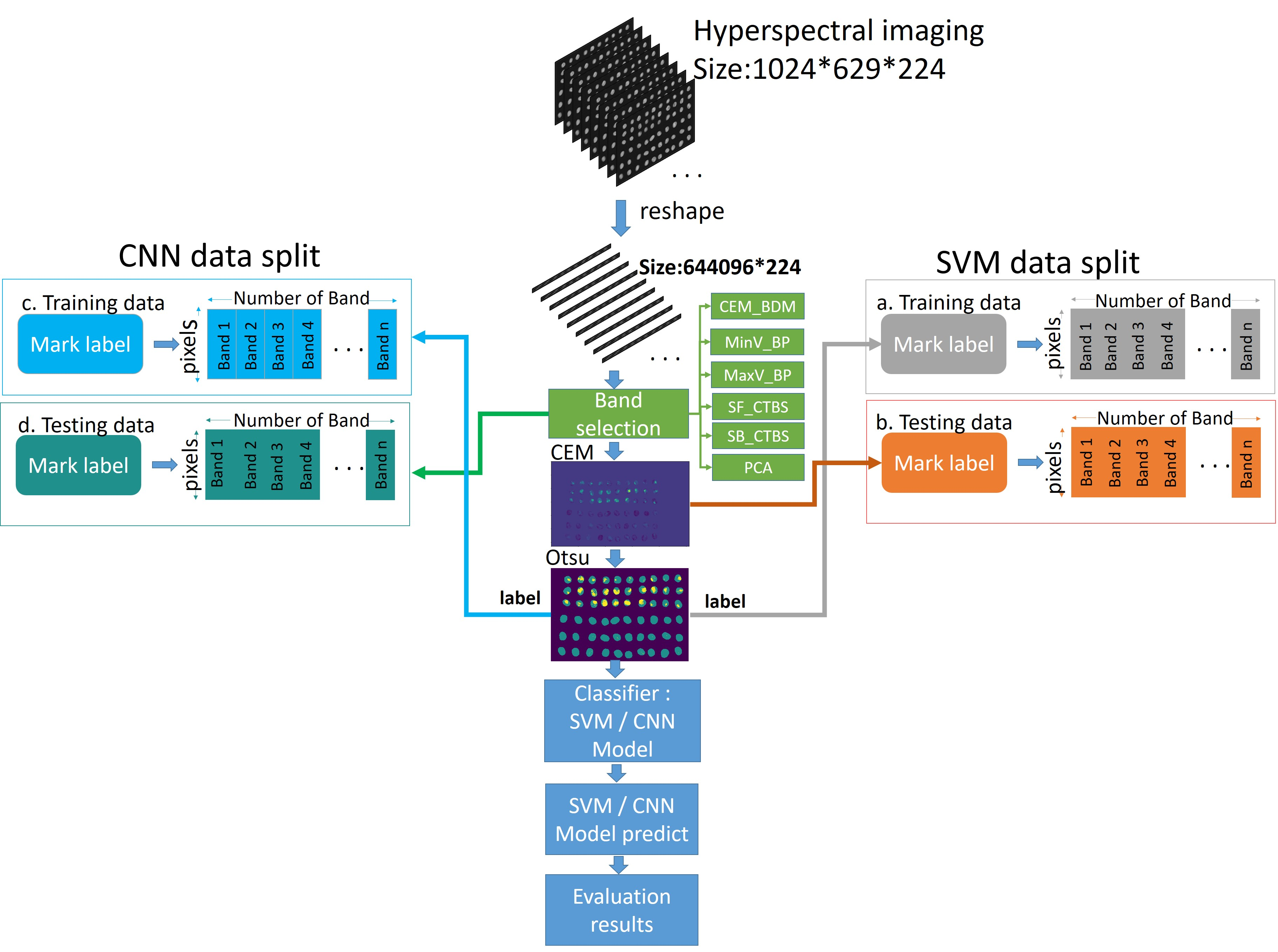
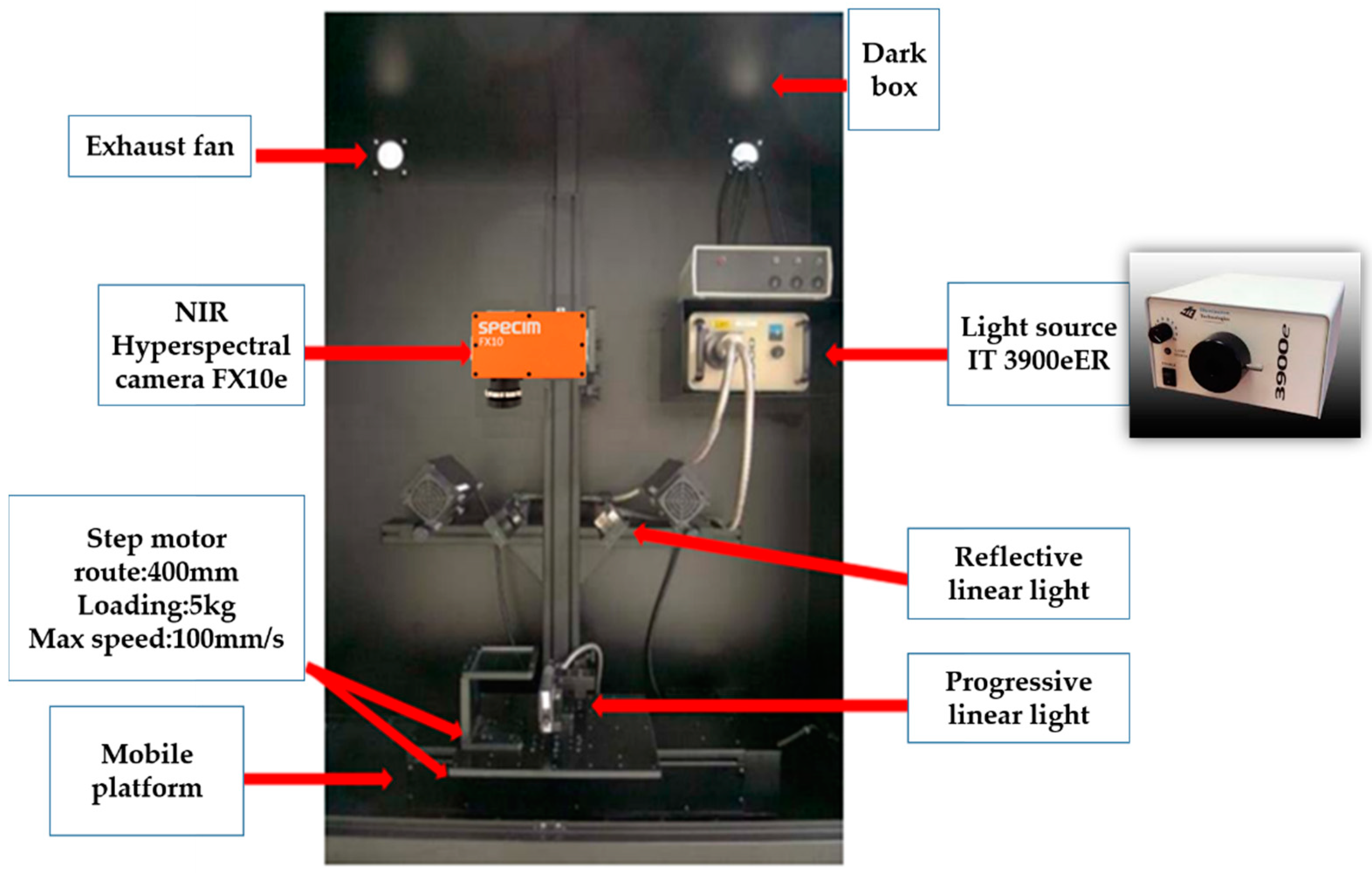
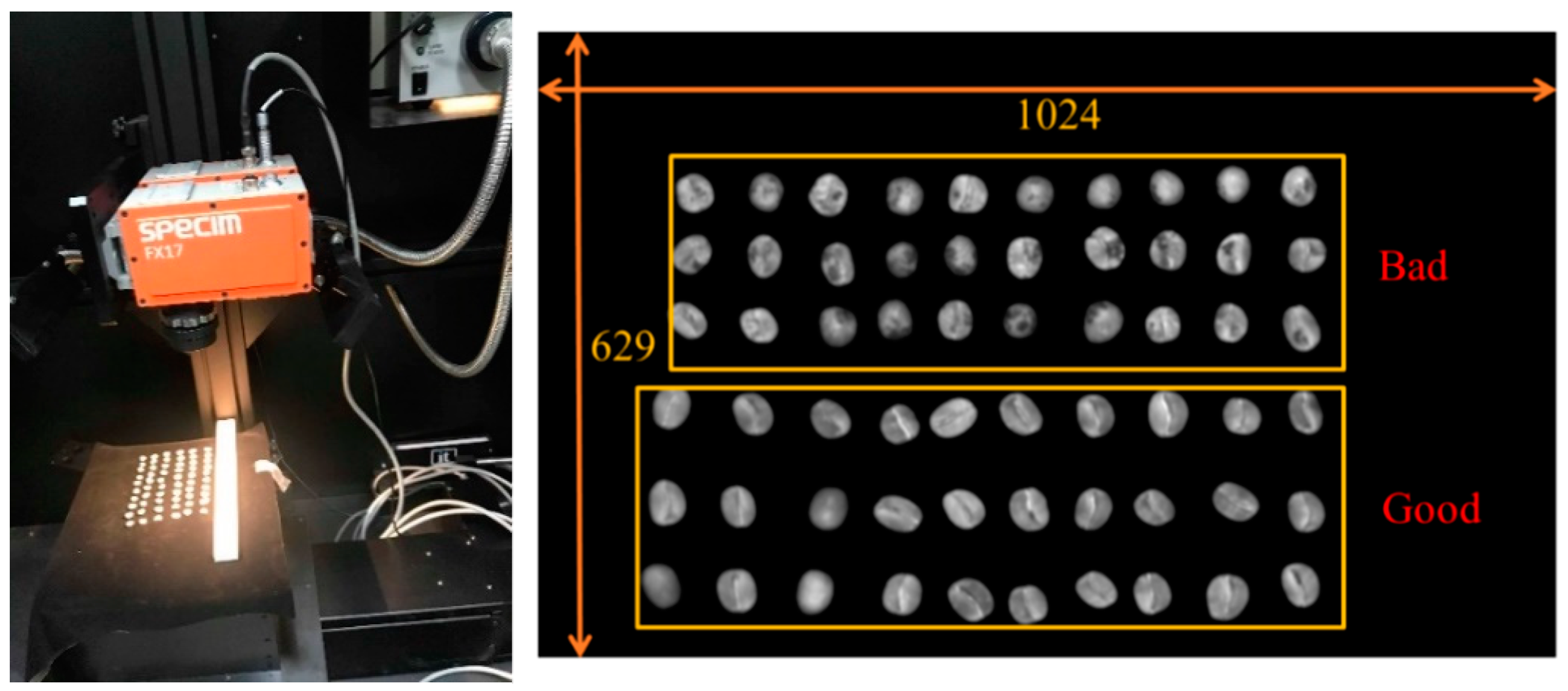
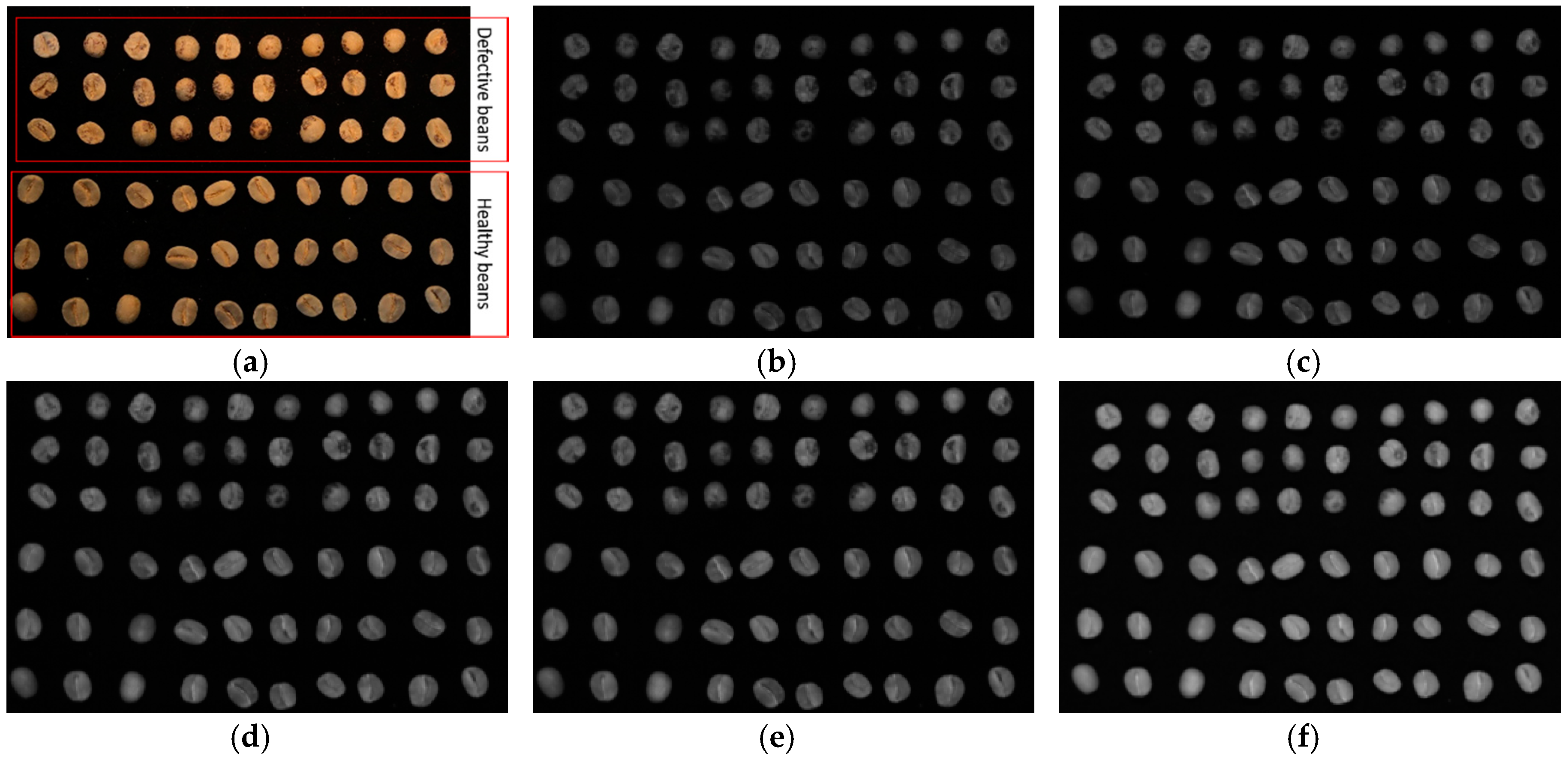
The hyperspectral push-broom scanning system (ISUZU Optics Corp.) used in this experiment is shown in Figure 1. A carried camera SPECIMFX10 hyperspectral sensor with a spectral range of 400–1000 nm, a resolution of 5.5 nm, and 224 bands was used for imaging. The light source for irradiating the images was “3900e-ER”, with a power of 21V/150W, comprised of a loading implement and mobile platform, and step motor (400 mm, maximum load: 5 kg, and maximum speed: 100 mm/s). The system was controlled with ISUZU software. The dark (closed shutter) and white (99% reflection spectrum) images were recorded and stored automatically before each measurement. The laboratory samples were placed on movable plates so that they were appropriately spaced. In each image, 60 green coffee beans were analyzed. The process of filming coffee beans is shown in Figure 2. Each time, 30 insect damaged beans and 30 healthy beans were filmed. Figure 3 shows the actual filming results. The mobile platform and correction whiteboard were located in the lower part, and the filming was performed in the dark box to avoid the interference from other light sources. The spectral signatures of green coffee beans were obtained after filming. Figure 3 shows the post-imaging hyperspectral images. The spectral range was 400–1000 nm. The hyperspectral camera captured 224 spectral images and the image data size was 1024 × 629 × 224.

2.2. Coffee Bean Samples

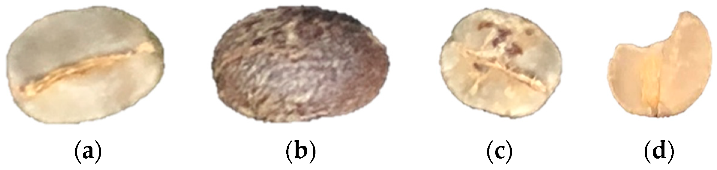
After the seeds produced by healthy coffee trees are removed, washed, sun-dried, fermented, dried, and shelled, healthy beans are then separated from defective beans. Common defective beans include black beans, insect damaged beans, and broken beans. Figure 4 shows the healthy and defective beans.

• Healthy beans: The entire post-processed bean should appear free of defects. The color of the beans should be blue-green, light green, or yellow-green, as shown in Figure 4a.
• Black beans: Black beans appear darkened before harvest or fully fermented, as shown in Figure 4b, and produce a turbid and putrefactive odor in coffee [7,8].
• Insect damaged beans: The insect damaged bean shown in Figure 4c is a result of coffee cherry bugs laying eggs on a coffee tree and the hatched larvae biting the coffee drupes to form wormholes. This type of defective bean produces a turbid odor or strange taste in coffee.
• Broken beans: Figure 4d shows a bean that was damaged during the treatment process or transportation, known as “ruptured beans”. It is likely to induce non-uniform baking [9].

The sample of coffee beans used this study were provided by coffee farmers in Yulin, Taiwan. The coffee farmers filtered the beans and provided both healthy and defective coffee bean samples for the experiment on coffee bean classification. In order to ensure the intactness of the sample beans, all beans were removed from the bag using tweezers, and the tweezers were wiped before touching different types of beans. A total of 1139 beans were collected, and 19 images were recorded. The quantities of the coffee beans are listed in

Table 2. Quantities from the experiment.

Class	Qty (pcs)
Healthy beans	569
Defective beans	570
Total	1139

.

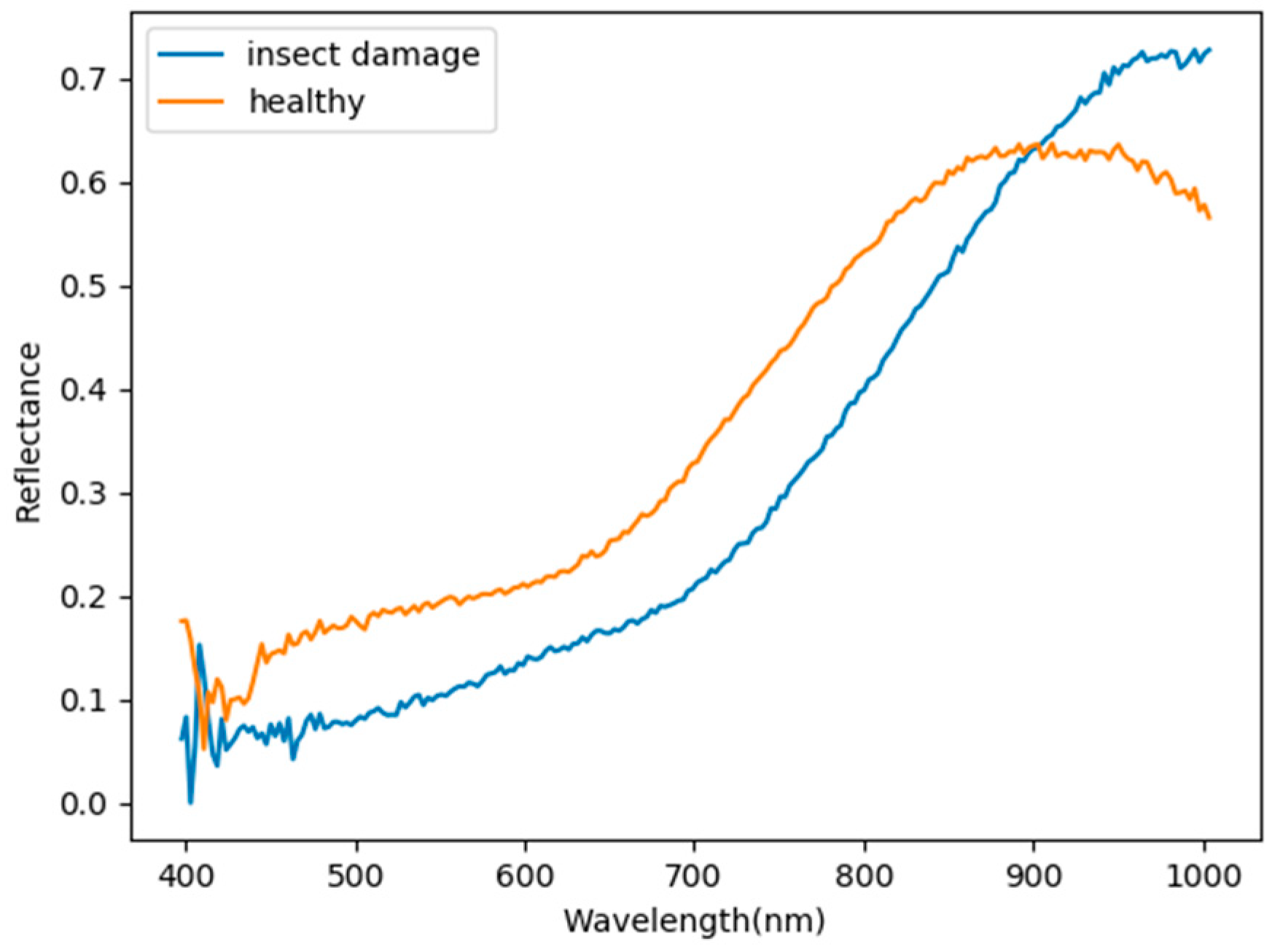
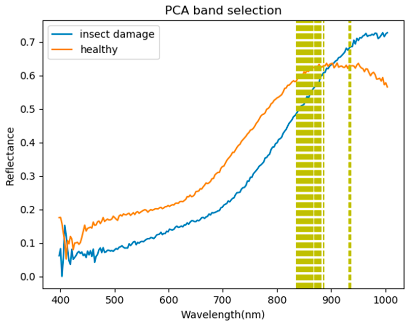
The hyperspectral data of green coffee beans and the original hyperspectral data were obtained, and 224 bands were observed after filming the green coffee beans in the spectral range of 400–1000 nm. The data were normalized to enhance the model convergence regarding the speed and precision of band selection with machine learning or deep learning. We collected 19 hyperspectral images in the experiments. Figure 5 shows the spectral signatures of the healthy beans and defective beans for our proposed hyperspectral algorithm.

2.3. Hyperspectral Band Selection

In hyperspectral imaging (HSI), hyperspectral signals, with as many as 200 contiguous spectral bands, can provide high spectral resolution. In other words, subtle objects or targets can be located and extracted by hyperspectral sensors with very narrow bandwidths for detection, classification, and identification. However, as the number of spectral bands and the inter-band information redundancy are usually very high in HSI, the original data cube is not suitable for data compression or data transmission, and particularly, image analysis. The use of full bands for data processing often encounters the issue of “the curse of dimensionality”; therefore, band selection plays a very important role in HSI. The purpose of band selection is to select the most representative set of bands in the image and include them in the data, so that they can be as close as possible to the entire image. Previous studies have used various band selection methods based on certain statistical criteria [10,11,12,13,14,15,16,17], mostly select an objective function first, and then select a band group that can maximize the objective function. This paper first used the histogram method in [18] to remove the background, and then applied six band selection methods based on constrained energy minimization (CEM) [19,20,21,22,23,24] to select and extract a representative set of bands.

2.3.1. Constrained Energy Minimization (CEM)

CEM [19,20,21,22,23,24] is similar to matched filtering (MF); the CEM algorithm only requires one spectral signature (desired signature or target of interest) as parameter d, while other prior knowledge (e.g., unknown signal or background) is not required. Basically, CEM applies a finite impulse response (FIR) filter to pass through the target of interest, while minimizing and suppressing noise and unknown signals from the background using a specific constraint. CEM suppresses the background by correlation matrix R, which can be defined as $R=(\raisebox{1ex}{$\mathbf{1}$}\!\left/ \!\raisebox{-1ex}{$N$}\right.){{\displaystyle \sum }}_{i=\mathbf{1}}^N{r}_i{r}_i{}^T$, and feature d is used by FIR to detect other similar targets. Assuming one hyperspectral image with N pixels r is defined as $\left\{r_{\mathbf{1}},r_{\mathbf{2}},r_{\mathbf{3}},\dots ,r_{\mathbf{N}}\right\}$, each pixel has L dimensions expressed as $r_i={(r_{i\mathbf{1}},r_{i\mathbf{2}},r_{i\mathbf{3}},\dots ,r_{iL})}^T$, thus, the desired target d can be defined as ${(d_{\mathbf{1}},d_{\mathbf{2}},d_{\mathbf{3}},\dots ,d_L)}^T$, and the desired target is passed through by the FIR filter. The coefficient in the finite impulse response filter can be defined as $\mathit{w}={({\mathit{w}}_{\mathbf{1}},{\mathit{w}}_{\mathbf{2}},{\mathit{w}}_{\mathbf{3}},\dots ,{\mathit{w}}_{\mathit{L}})}^{\mathit{T}}$, where the value of w can be obtained by the constrain ${\mathit{d}}^{\mathit{T}}w={\mathit{w}}^{\mathit{T}}\mathit{d}=\mathbf{1}$, and the result of CEM is:

$${\mathsf{\delta }}^{\mathrm{CEM}}={({\mathrm{w}}^{\mathrm{CEM}})}^{\mathrm{T}}\mathrm{r}={({\mathrm{d}}^{\mathrm{T}}{\mathrm{R}}_{\mathrm{L}\times \mathrm{L}}^{-1}\mathrm{d})}^{-1}{({\mathrm{R}}_{\mathrm{L}\times \mathrm{L}}^{-1}\mathrm{d})}^{\mathrm{T}}\mathrm{r}$$

(1)

CEM is one of the few algorithms that can suppress the background while enhancing the target at the subpixel level. CEM is easier to implement than binary classification as it uses the sampling correlation matrix R to suppress BKG, thus, it only requires meaningful knowledge of the target and no other information is required. In this regard, CEM has been used to design a new band selection method called constraint band selection (CBS) [19], and the resulting minimum variance from CBS is used to calculate the priority score to rank the frequency bands. Conceptually, constrained-target band selection (CTBS) [25,26] is slightly different from CBS, as CBS only focuses on the band of interest, while CTBS simultaneously takes advantage of the target signature and the band of interest. First, it specifies the signal d of a target, and then constrains d to minimize the variance caused by the background signal through the FIR filter. The resulting variance can also be selected by the selection criteria. Since CEM has been widely used for subpixel target detection in hyperspectral imagery, this paper applied CBS and CTBS based methods for further analysis. The following are the six target detection based band selection methods used in the experiments.

2.3.2. Constrained Energy Minimization-Constrained Band Dependence Minimization (CEM-BDM)

CEM-BDM [19] is one of the CBS methods, which uses CEM to determine the correlation between the various bands, and regards such correlation as a score. Subsequent processing is then performed on this score to obtain a band selection algorithm with different band priorities. Let $\left\{B_{\mathit{l}}\right\}$ be the set of all band images, where $\left\{b_{\mathit{l}}\right\}$ denotes each band image sized at M $\times$ N in a hyperspectral image cube. A optimization problem similar to CEM can be obtained for a constrained band-selection problem by $\underset{w_l}{\min }\left\{{\mathit{w}}_{\mathit{l}}{}^{\mathit{T}}\mathit{Q}{\mathit{w}}_{\mathit{l}}\right\} subject to {\mathit{b}}_l{}^T{\mathit{w}}_{\mathit{l}}=1$, which uses the least squares error (LSE) as the constraint. CEM-BDM can be extended as follows: assume the autocorrelation matrix as $\tilde{\mathit{Q}}=\frac{1}{L-1}{{\displaystyle \sum }}_{j=1,j\ne l}^L{\mathit{b}}_j{\mathit{b}}_j{}^T$ and the coefficient in the finite impulse response filter as ${\tilde{\mathit{w}}}_l^{CEM}={({\mathit{b}}_l{}^T{\tilde{\mathit{Q}}}^{-1}{\mathit{b}}_{\mathit{l}})}^{-1}{\tilde{\mathit{Q}}}^{-1}{\mathit{b}}_{\mathit{l}},$ thus, the final results of CEM-BDM can be defined as follows:

$$BD{M}_{priority}({\mathit{B}}_{\mathit{l}})={({\tilde{\mathit{w}}}_l^{CEM})}^T\tilde{\mathit{Q}}{\tilde{\mathit{w}}}_l^{CEM}$$

(2)

This band selection method uses the least square error to determine the correlation between the bands. If the results of the least square error are larger, it means that the current band is more dependent on other bands, and thus, the more significant band.

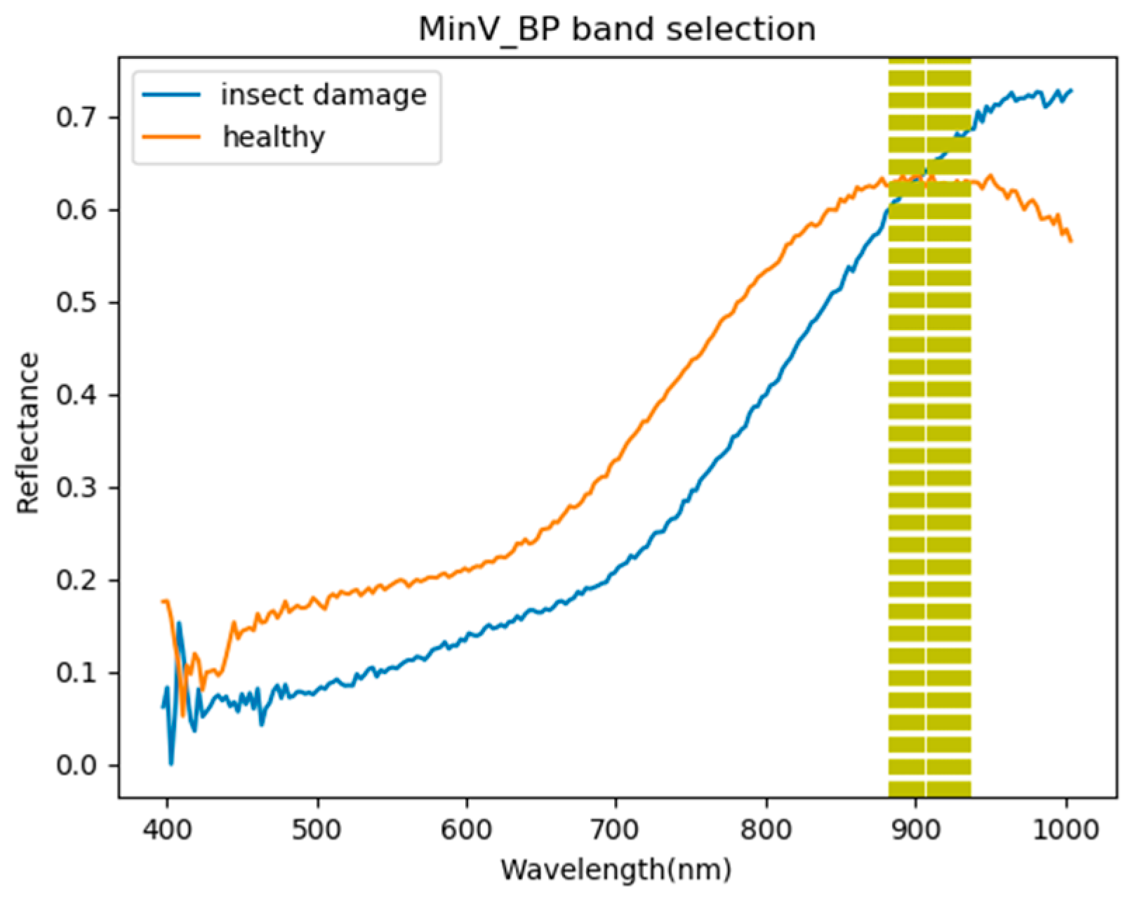
2.3.3. Minimum Variance Band Prioritization (MinV-BP)

According to the optimization method of CEM, the priority score is processed by the variance value; the smaller the variance, the higher the priority score. CEM ranks bands by starting with the minimal variance as its first selected band. Let ${\left\{{\mathit{b}}_{\mathit{l}}\right\}}_{\mathrm{l}=1}^L$ be the total band images for a hyperspectral image cube, where ${\mathit{b}}_{\mathit{l}}$ is the lth band in the image. By applying CEM, this value is obtained by the full band set $\mathrm{\Omega },V(\Omega )={({\mathit{d}}_{\mathrm{\Omega }}^T{\mathit{R}}_{\mathrm{\Omega }}^{-1}{\mathit{d}}_{\mathrm{\Omega }})}^{-1}={({\mathit{d}}^{\mathit{T}}{\mathit{R}}^{-\mathbf{1}}\mathit{d})}^{-1}$, in this case, for each single band ${\mathit{b}}_{\mathit{l}}$, the MinV-BP [23,25,26] variance can be defined as:

$$\mathrm{V}({\mathit{b}}_{\mathit{l}})={({\mathit{d}}_{{\mathit{b}}_{\mathit{l}}}^T{\mathit{R}}_{{\mathit{b}}_{\mathit{l}}}^{-1}{\mathit{d}}_{{\mathit{b}}_{\mathit{l}}})}^{-1}$$

(3)

This can be used as a measure of variance, as it uses only the data sample vector specified by ${\mathit{b}}_{\mathit{l}}$. Therefore, the value of $\mathrm{V}({\mathit{b}}_{\mathit{l}})$ can be further used as the priority score of ${\mathit{b}}_{\mathit{l}}$. According to this explanation, the band is ranked by the value of $\mathrm{V}({\mathit{b}}_{\mathit{l}})$; the smaller the $\mathrm{V}({\mathit{b}}_{\mathit{l}})$, the higher the priority of band selection.

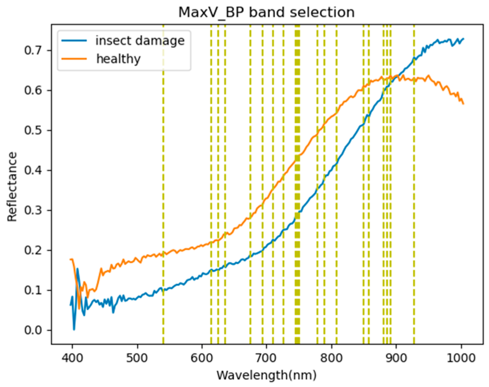
2.3.4. Maximum Variance Band Prioritization (MaxV-BP)

In contrast to MinV-BP, the concept of Max V-BP [23,25] is to first remove ${\mathit{b}}_{\mathit{l}}$ from the band set Ω, and the variance is calculated as follows:

$$\mathrm{V}(\Omega -b_l)={({\mathit{d}}_{\Omega -\left\{b_{\mathit{l}}\right\}}^{\mathit{T}}{\mathit{R}}_{\Omega -\left\{b_{\mathit{l}}\right\}}^{-\mathbf{1}}{\mathit{d}}_{\Omega -\left\{b_{\mathit{l}}\right\}})}^{-1}$$

(4)

Under this criterion, the value of $\mathrm{V}(\Omega -b_{\mathit{l}})$ can also be the measurement of the priority score for $b_l$ Consequently, ${\left\{{\mathit{b}}_{\mathit{l}}\right\}}_{l=1}^L$ can be ranked by the decreasing values of $\mathrm{V}(\Omega -b_{\mathit{l}})$. The maximum $\mathrm{V}(\Omega -b_{\mathit{l}})$ is supposed to be the most significant, and the band is prioritized by (4). The difference between MinV_BP and MaxV_BP is that MinV_BP conducts sorting according to a single band, while MaxV_BP is sorted by the full band, and the results of the two band selections are not opposite.

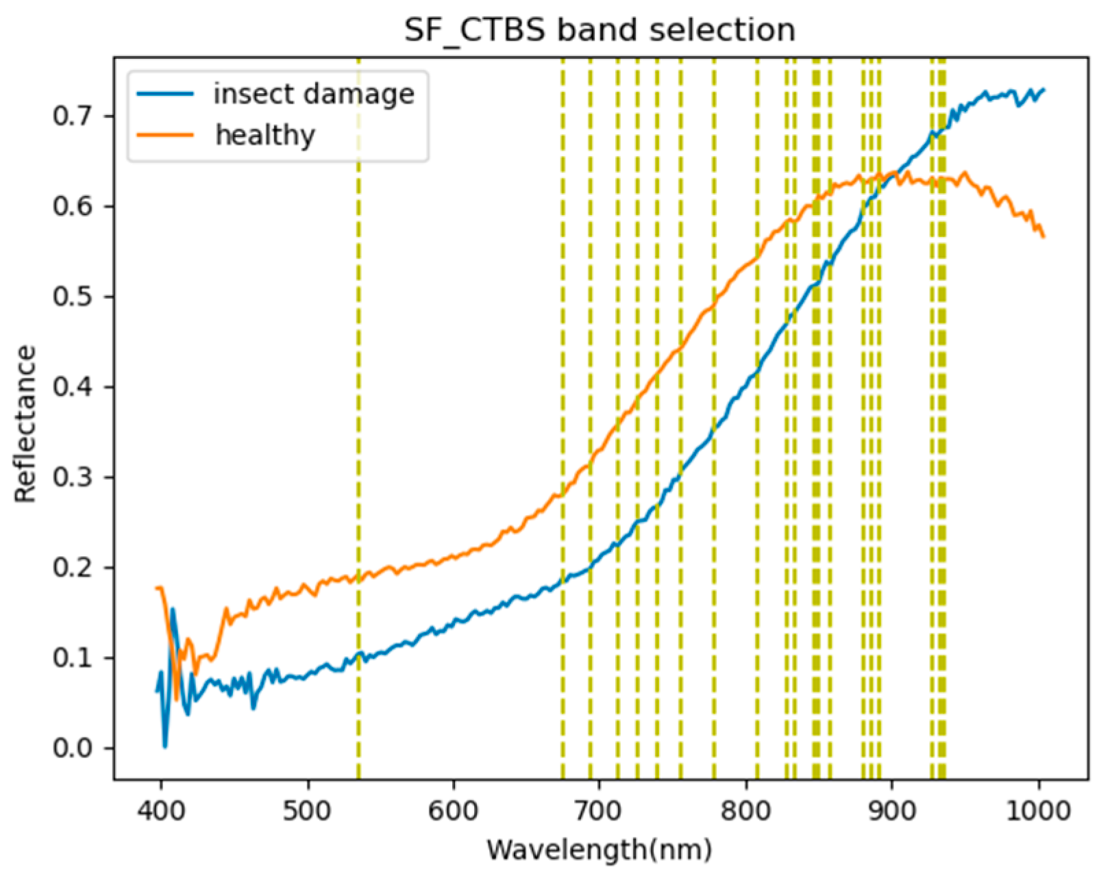
2.3.5. Sequential Forward-Constrained-Target Band Selection (SF-CTBS)

SF-CTBS [25] uses the MinV_BP criteria in (3) to select one band at a time sequentially, instead of sorting all bands with the scores in (3), as MinV_BP does. As a result, band ${\mathit{b}}_{l_1}^{*}$ can obtain the minimal variance.

$${\mathit{b}}_{l_1}^{*}=\arg \left\{{}_{{\mathit{b}}_{\mathit{l}}\in \Omega }{}^{min}V({\mathit{b}}_l)\right\}=\arg \left\{{}_{b_l\in \mathrm{\Omega }}{}^{min}({\mathit{d}}_{{\mathit{b}}_{\mathit{l}}}^{\mathit{T}}{\mathit{R}}_{{\mathit{b}}_{\mathit{l}}}^{-\mathbf{1}}{\mathit{d}}_{{\mathit{b}}_{\mathit{l}}}){}^{-1}\right\}$$

(5)

$\mathrm{where} b_{l_1}^{*}$ is the first selected band, and the second band is generated by another minimum variance

$${\mathit{b}}_{l_2}^{*}=\arg \left\{{}_{{\mathit{b}}_{\mathit{l}}\in \Omega -{\mathit{b}}_{{\mathit{l}}_{\mathbf{1}}}^{}}{}^{min}V({\mathit{b}}_l)\right\}=\arg \left\{{}_{{\mathit{b}}_{\mathit{l}}\in \Omega -{\mathit{b}}_{{\mathit{l}}_{\mathbf{1}}}^{}}{}^{min}({\mathit{d}}_{{\mathit{b}}_{\mathit{l}}}^{\mathit{T}}{\mathit{R}}_{{\mathit{b}}_{\mathit{l}}}^{-\mathbf{1}}{\mathit{d}}_{{\mathit{b}}_{\mathit{l}}}){}^{-1}\right\}$$

(6)

This process is repeated continuously by adding each newly selected band, while the sequential forward technique in [26,27] selects one band at a time sequentially.

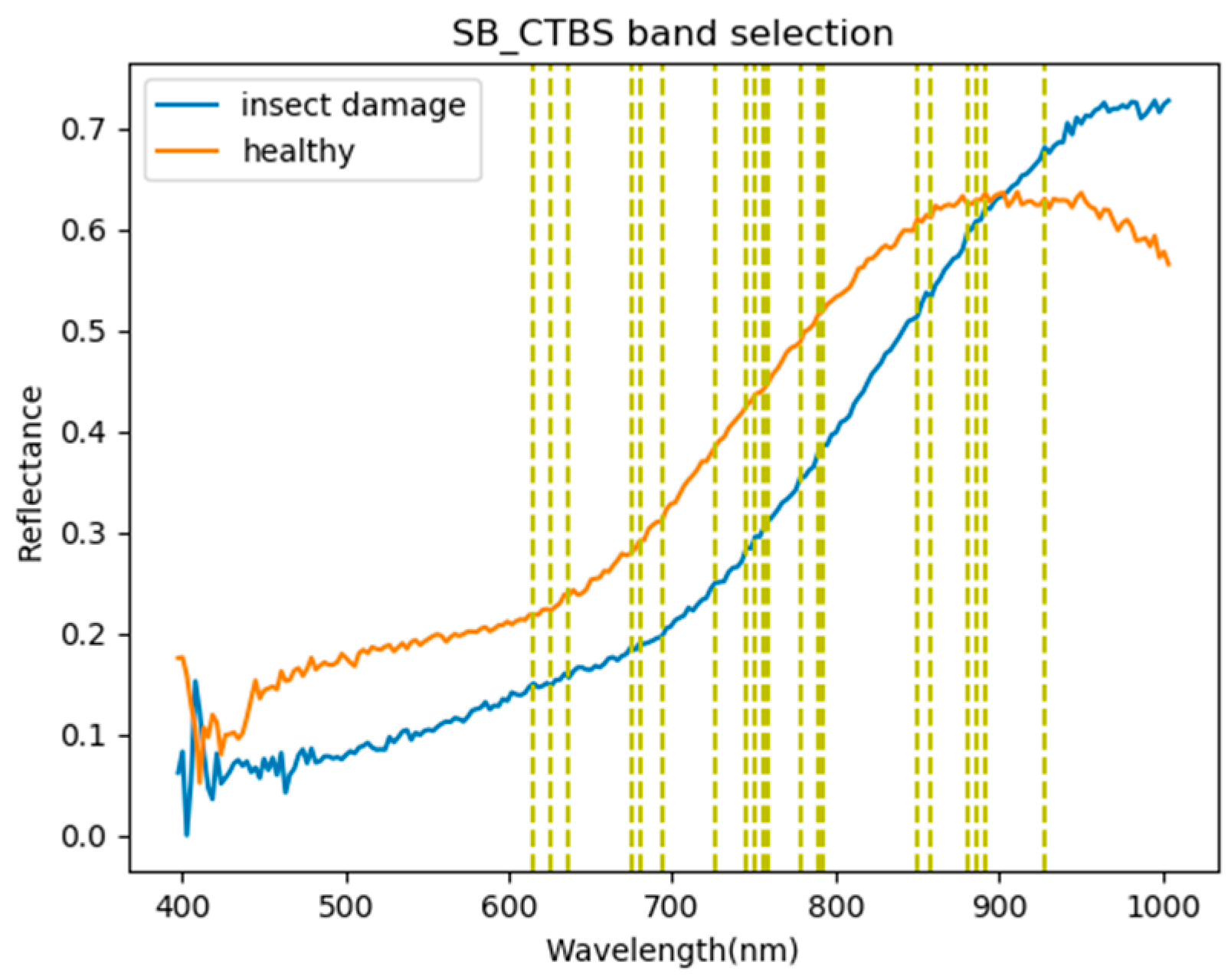
2.3.6. Sequential Backward-Target Band Selection (SB-CTBS)

In contrast to SF-CTBS using the MinV_BP criteria in (3), SB-CTBS [25] applies the MaxV_BP as the criterion by using the leave-one-out method to select the optimal bands. For each single band, $b_{\mathit{l}}$, assumes band subset $\Omega -{\mathit{b}}_{{\mathit{l}}_{\mathbf{1}}}^{},$ which removes $b_{\mathit{l}}$ from the full band. The first selected band can be obtained by (7), which yields the maximal variance and ${\mathit{b}}_{l_1}^{*}$ can be considered as the most significant band.

$${\mathit{b}}_{{\mathit{l}}_{\mathbf{1}}}^{*}=\arg \left\{{}_{{\mathit{b}}_{\mathit{l}}\in \Omega }{}^{max}V(\Omega -\left\{{\mathit{b}}_{\mathit{l}}\right\})\right\}=\arg \left\{{}_{{\mathit{b}}_l\in \mathrm{\Omega }}{}^{max}({\mathit{d}}_{\Omega -\left\{{\mathit{b}}_{\mathit{l}}\right\}}^{\mathit{T}}{\mathit{R}}_{\Omega -\left\{{\mathit{b}}_{\mathit{l}}\right\}}^{-\mathbf{1}}{\mathit{d}}_{\Omega -\left\{{\mathit{b}}_{\mathit{l}}\right\}}){}^{-1}\right\}$$

(7)

After calculating ${\mathit{b}}_{l_1}^{*}$, we can have ${\mathrm{\Omega }}_1=\mathrm{\Omega }-\left\{b_{l_1}\right\}$, and the second band can be generated by another maximal variance in (8). The same process is repeated continuously by removing the current selected band one at a time from the full band set.

$${\mathit{b}}_{{\mathit{l}}_{\mathbf{2}}}^{*}=\arg \left\{{}_{{\Omega }_{\mathbf{1}}-\left\{{\mathit{b}}_{\mathit{l}}\right\}}{}^{max}V({\Omega }_{\mathbf{1}}-\left\{{\mathit{b}}_{\mathit{l}}\right\})\right\}=\arg \left\{{}_{{\Omega }_{\mathbf{1}}-\left\{{\mathit{b}}_{\mathit{l}}\right\}}{}^{max}({\mathit{d}}_{{\Omega }_{\mathbf{1}}-\left\{{\mathit{b}}_{\mathit{l}}\right\}}^{\mathit{T}}{\mathit{R}}_{{\Omega }_{\mathbf{1}}-\left\{{\mathit{b}}_{\mathit{l}}\right\}}^{-1}{\mathit{d}}_{{\Omega }_{\mathbf{1}}-\left\{{\mathit{b}}_{\mathit{l}}\right\}}){}^{-1}\right\}$$

(8)

It can be noted that the differences between SB-CTBS and SF-CTBS are that SB-CTBS removes bands from the full band set to generate a desired selected band subset, while SF-CTBS increases the selected band by calculating the minimal variance one at a time. The correlation matrix in SB-CTBS uses ${{R}}_{\mathrm{\Omega }-\left\{b_l\right\}}$ but the correlation matrix in SF-CTBS is ${{R}}_{b_l}^{}$.

2.3.7. Principal Component Analysis (PCA)

PCA [28] is classified in machine learning as a method of feature extraction in dimensional reduction, and can be considered as an unsupervised linear transformation technology, which is widely used in different fields. Dimensionality reduction is used to reduce the number of dimensions in data, without much influence on the overall performance. The basic assumption of PCA is that the data can identify a projection vector, which is projected in the feature space to obtain the maximum variance of this dataset. In this case, this paper compared PCA with other CEM-based band selection methods.

2.4. Optimal Signature Generation Process

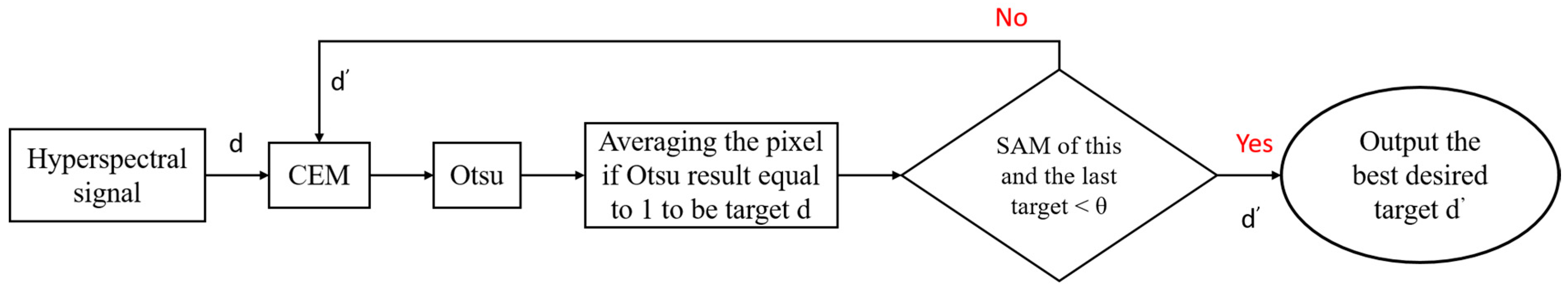
Our proposed algorithm first identified the desired signature of insect damaged beans as the d (desired signature) in CEM for the detection of other similar beans. Optimal signature generation process (OSGP) [29,30] was used to find the optimal desired spectral signature. As the CEM needs only one desired spectral signature for detection, the quality of the detection result is very sensitive to the desired spectral signature. To minimize this defect, the OSGP selects the desired target d first, and the CEM is repeated to obtain a stable and better d. Thus, the stability of detection can be increased, and the subsequent CEM gives the best detection result. Figure 6 shows the flow diagram of OSGP, and then Otsu’s method [31] is used to find the optimal threshold. Otsu’s method divides data into 0 and 1. This step is to label data for follow-up analysis.

2.5. Convolutional Neural Networks (CNN)

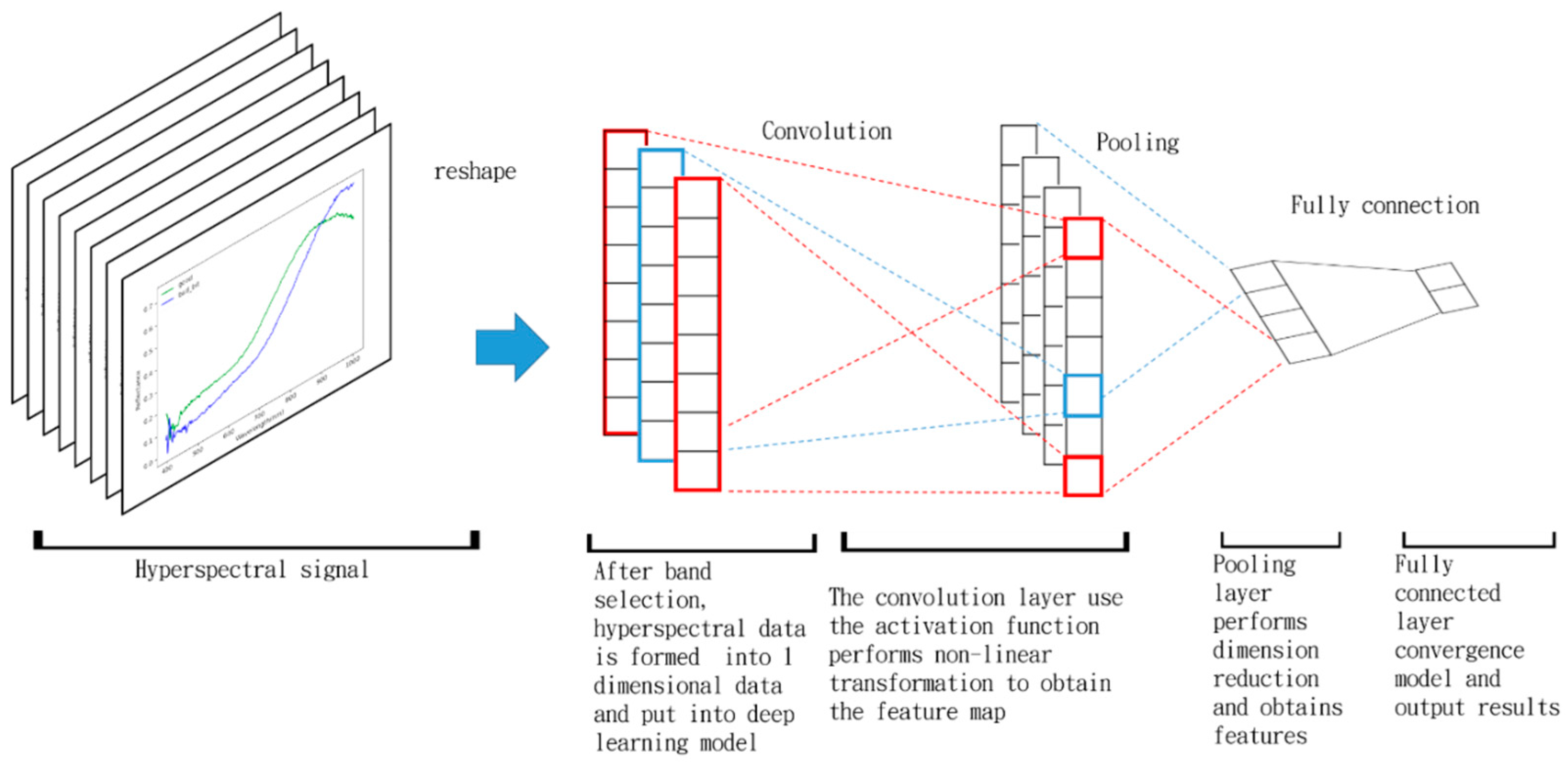
Feature extraction requires expert knowledge as the important features must be known for this classification problem, and are extracted from the image to conduct classification. The “convolution” in convolutional neural network (CNN) [32,33,34,35,36,37,38] refers to a method of feature extraction, which can replace experts to extract features. Generally speaking, CNN effectively uses spatial information in traditional RGB images; for example, 2D-CNN uses the shape and color of the target in the image to capture features. However, insect damaged coffee beans may be mixed with other material substances, and may even be embedded in a single pixel as their size is smaller than the ground sampling distance. In this case, as no shape or color can be captured, spectral information is important in the detection of insect damaged areas. Therefore, this paper used the pixel based 1D-CNN model to capture the spectral features, instead of spatial features. The result after the band selection of the hyperspectral image was molded into one-dimensional data and the context of data still existed, as shown in Figure 7. The 1D-CNN uses much fewer parameters than 2D-CNN and is more accurate and faster [39].

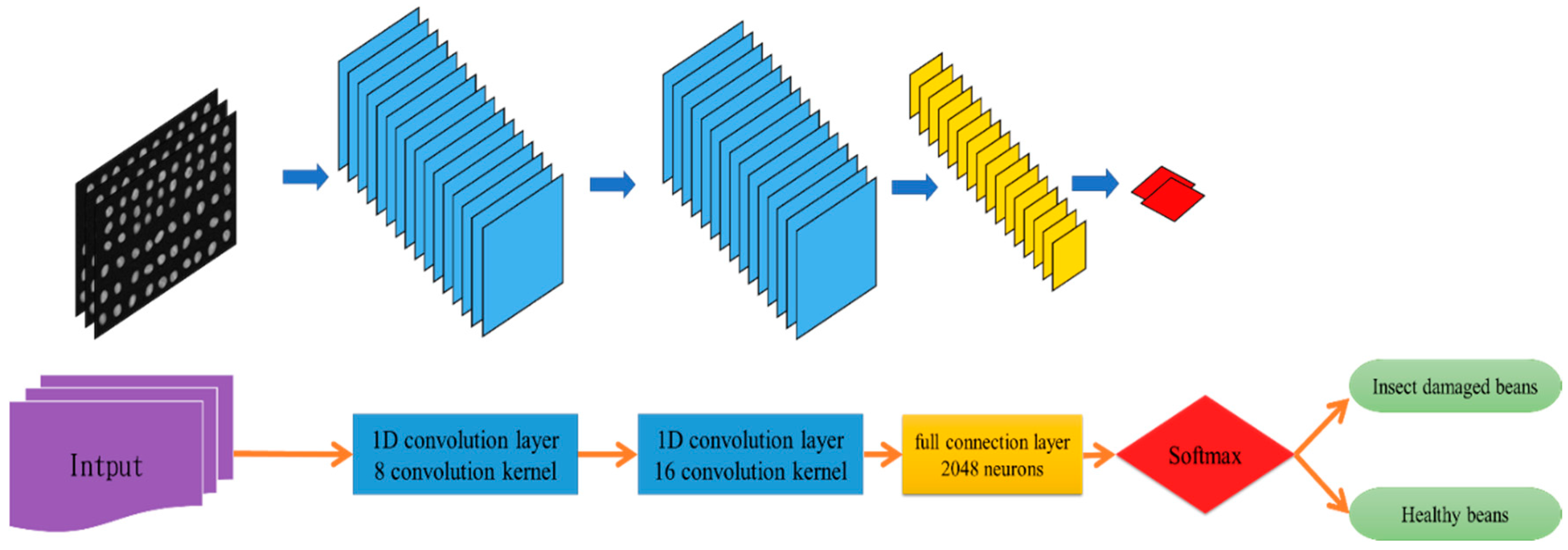
Figure 8 shows the 1D-CNN model architecture used in this paper. The hyperspectral image after band selection was used for further analysis, and the data size of the image was 1024 $\times$ 629. The features were extracted by using the convolution layer. An 8-convolution kernel and a 16-convolution kernel were used, and then 2048 neurons entered the full connection layer directly.

The network terminal was provided with a Softmax classifier, and the classifier result of the input spectrum was obtained. The parameters included the training test split: 0.33, epochs: 200, kernel size: 3, activation = ‘relu’, optimizer: SGD, Ir: 0.0001, momentum: 0.9, decay: 0.0005, factor = 0.2, patience = 5, min_lr = 0.000001, batch_size = 1024, and verbose = 1.

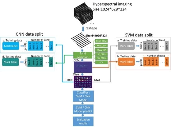
2.6. Hyperspectral Insect Damage Detection Algorithm (HIDDA)

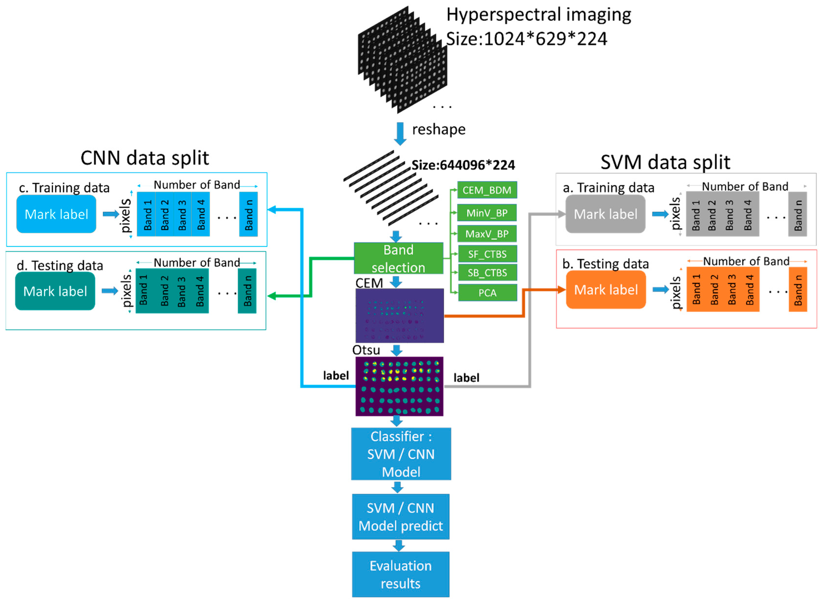
This paper combined the above methods to develop the hyperspectral insect damage detection algorithm (HIDDA), in which band selection is first used to filter out the important bands, and then CEM-OTSU is applied to generate training samples for the two classifiers, in order to implement binary classification for healthy and defective coffee beans. Method 1 uses linear support vector machine (SVM) [39], where the data are labeled and added for the classification of the coffee beans. While Otsu’s method was used for subsequent classification, considering its possible misrecognition, this paper improved classification with SVM. Method 2 is comprised of CNN. Figure 9 describes the HIDDA flowchart, which is divided into two stages: training (Figure 9a,c) and testing (Figure 9b,d).

In the training process, the spectral signature of an insect damaged bean was imported into the CEM as the desired target. The positions of other insect damaged beans could be detected automatically by Otsu’s method, and the result was taken as the training data of SVM and CNN (Figure 9a,c) to classify the remaining 19 images (Figure 9b,d). The training set and the test set of the CNN converted data into 1D data. The training data of this experiment were trained by acquiring the hyperspectral image of 60 coffee beans containing 30 insect damaged beans and 30 healthy beans simultaneously after obtaining the results of CEM-OTSU. The remaining 19 hyperspectral images were used for prediction, so the training samples were less than 5% and testing data were about 95%. The data were preprocessed before this experiment by using data normalization and background removal. Then, six band selection algorithms were used to find the sensitive bands of the insect damaged and healthy beans, and the hyperspectral algorithm CEM was performed. As the CEM only needs a single desired spectral signature for detection, this spectral signature is quite important in the algorithm. The best-desired signature was found by OSGP; this signature was put in CEM for analysis, and Otsu’s method divided the data into 0 and 1 to label the training data. This paper analyzed pixels instead of images, so this step is relatively important. The remaining 19 images of the test sets were used for SVM (Figure 9b), which used the CEM result for classification. The same set of 19 images after band selection was used as the CNN testing set (Figure 9d). As CNN used the convolution layer to extract features, CEM was not required for analysis. It can be noted that HIDDA generated training samples from the result of CEM-OTSU and not from prior knowledge, as the only prior knowledge HIDDA requires is a single desired spectral signature for CEM in the beginning.

3. Results and Discussion

3.1. Band Selection Results

According to Figure 9, the experimental hyperspectral data removed the background from the image before band selection. This experiment used six kinds of band selection (as discussed earlier) for comparison (minimum CEM-BDM, MinV-BP, MaxV-BP, SF-CTBS, SB-CTBS, and PCA. The SVM and CNN classifiers were then used for classification. Finally, the confusion matrix [40] and kappa [41,42] were used for evaluation and comparison. Instead of using pixels for evaluation, this paper used coffee beans as a unit; if a pixel of a coffee bean was identified as an insect damaged bean, it was classified as an insect damaged bean, and vice versa. In the confusion matrix of this experiment, TP represents a defective bean hit, FN is defective bean misrecognition, TN is healthy bean hit, and FP is healthy bean misrecognition. Figure 10, Figure 11, Figure 12, Figure 13, Figure 14 and Figure 15 show the graphics of the first 20 bands selected by band selection and after band selection. As per sensitive bands selected by six kinds of band selection, 3, 10, and 20 bands were used for the test. The bands after 20 were not selected because excessive bands can cause disorder and repeated data. In addition, excessive bands could make future hardware design difficult. Therefore, the number of bands was controlled below 20. According to the results in Figure 10, Figure 11, Figure 12, Figure 13, Figure 14 and Figure 15, almost all the foremost bands fell in the range of 850–950 nm. This finding helps to reduce cost and increase the use-value for future sensor design.

According to the results in Figure 10, Figure 11, Figure 12, Figure 13, Figure 14 and Figure 15, almost all the foremost bands fell in the wavelength range of 850–950 nm.

Table 3. Most frequently selected bands by six band selection algorithms in the first 20 bands. (●: include, X: not include).

Band	BDM	MinV_BP	MaxV_BP	SF_CTBS	SB_CTBS	PCA	Total Times
850 nm	●	X	●	●	●	●	5
886 nm	X	●	●	●	●	●	5
858 nm	X	X	●	●	●	●	4
933 nm	●	●	X	●	X	●	4
891 nm	X	●	●	●	●	X	4
880 nm	X	X	●	●	●	●	4
927 nm	X	●	●	●	●	X	4

lists the most frequently selected bands according to the six band selection algorithms in the first 20 bands, and 850 nm and 886 nm were selected by five out of six band selection algorithms, which means those bands are discriminate bands for coffee beans. This finding can help to reduce costs and increase the usage-value for future sensor designs.

3.2. Detection Results by Using Three Bands

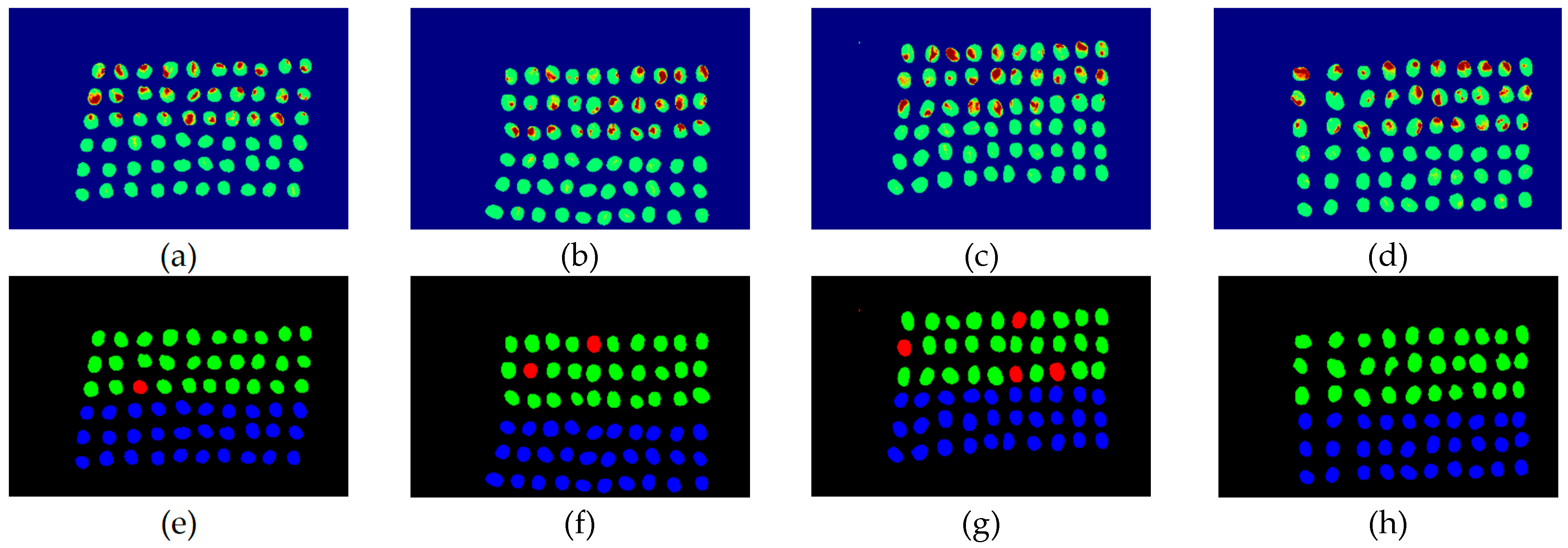
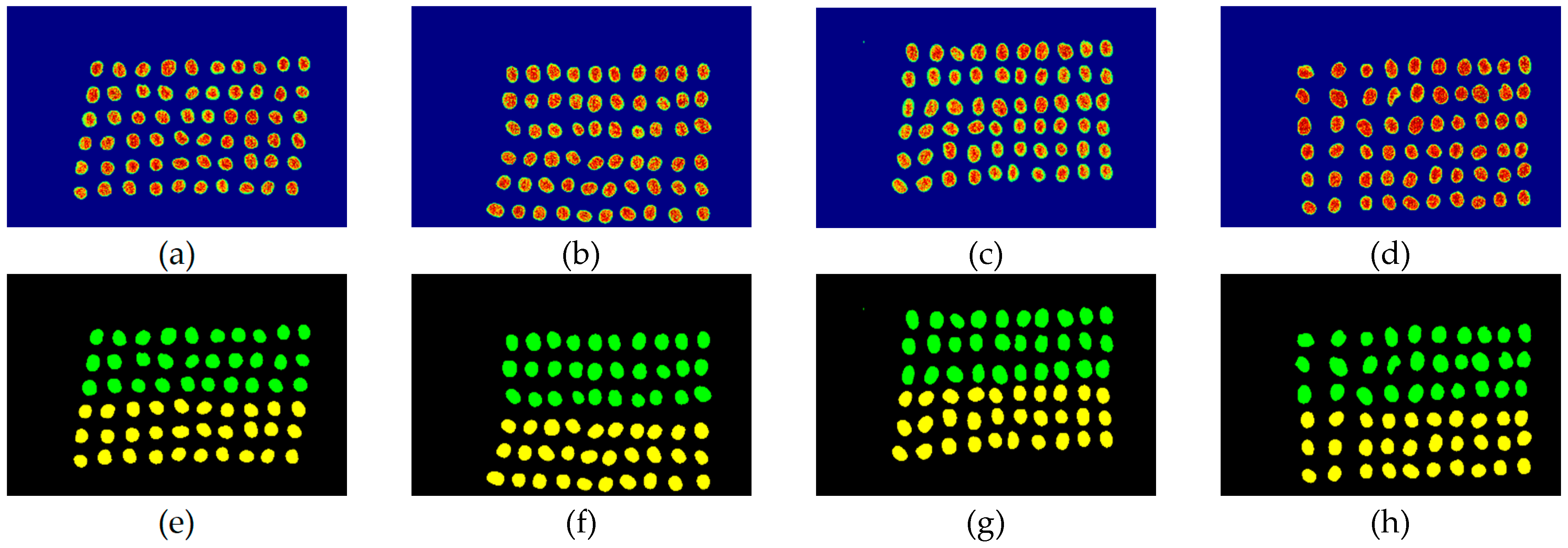
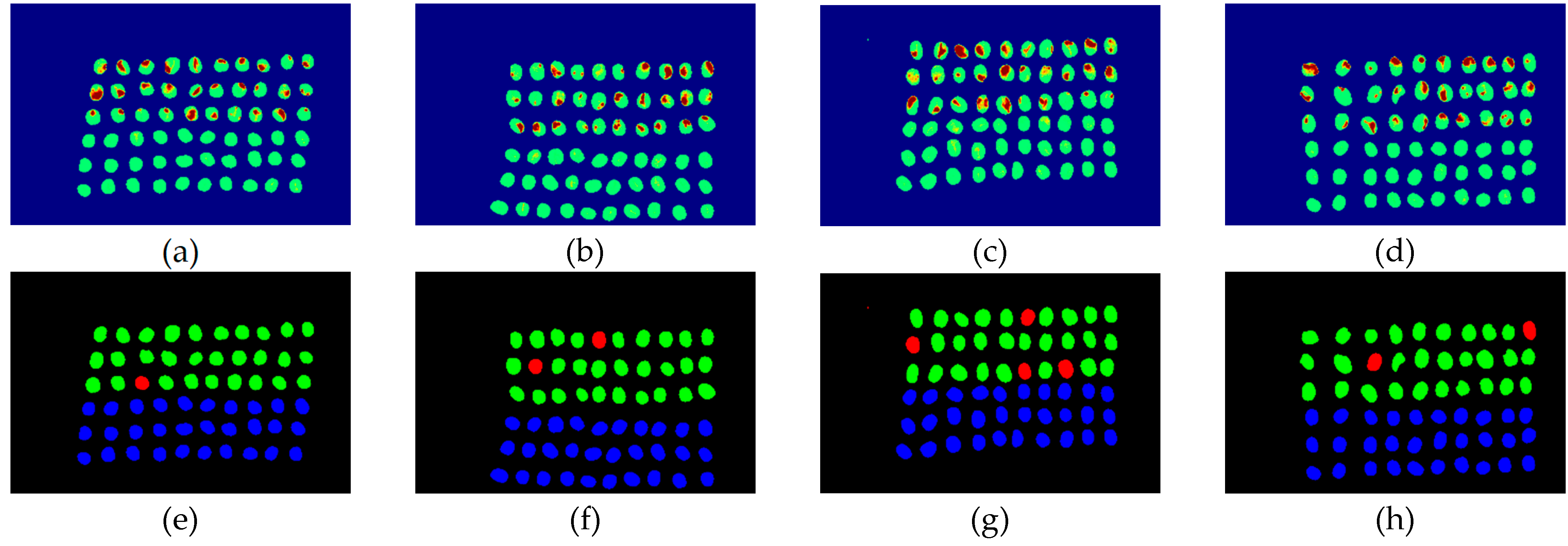
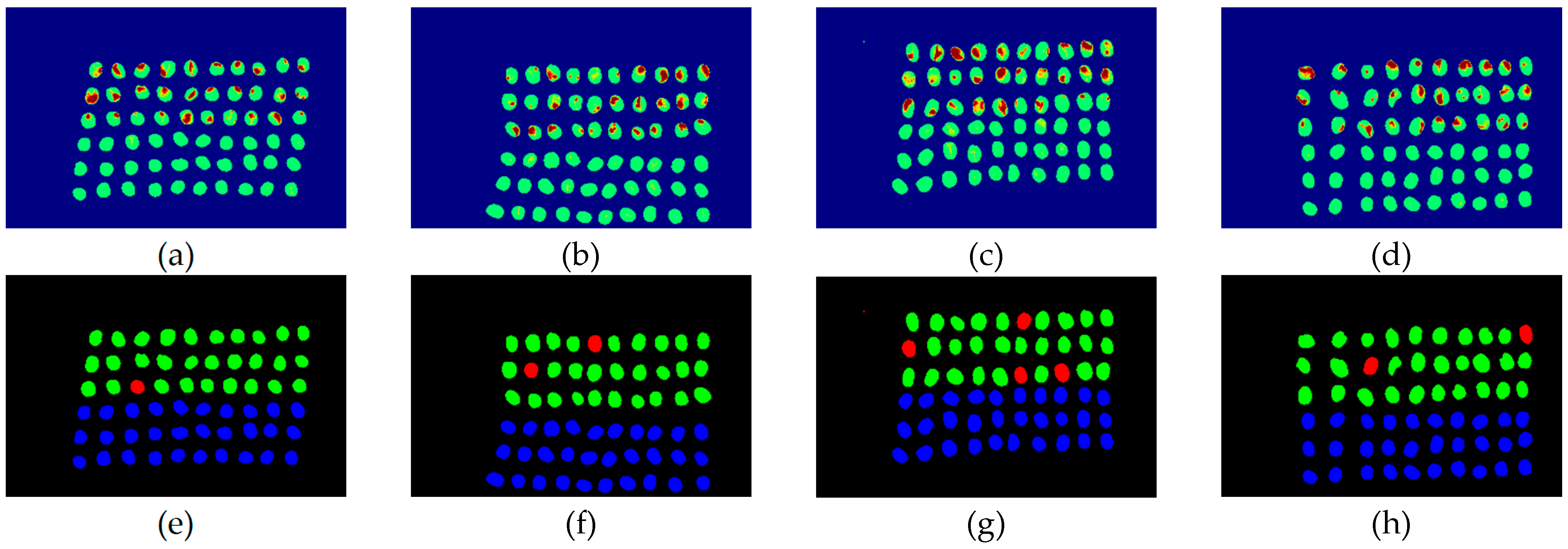
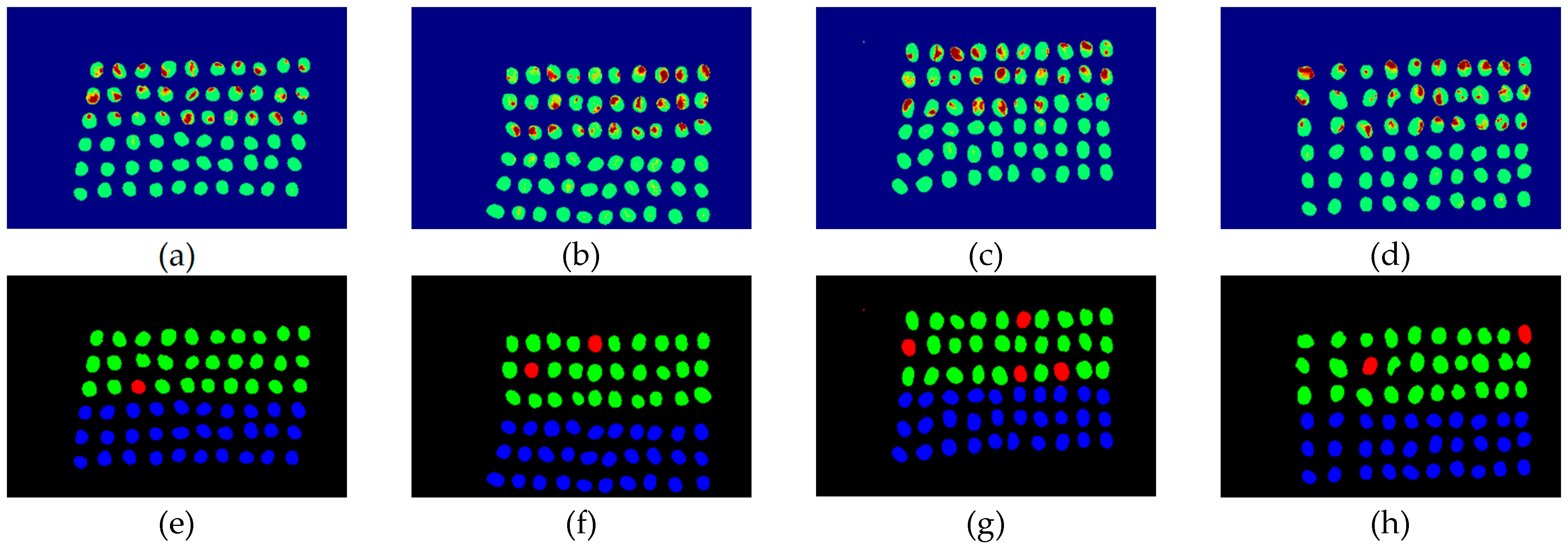
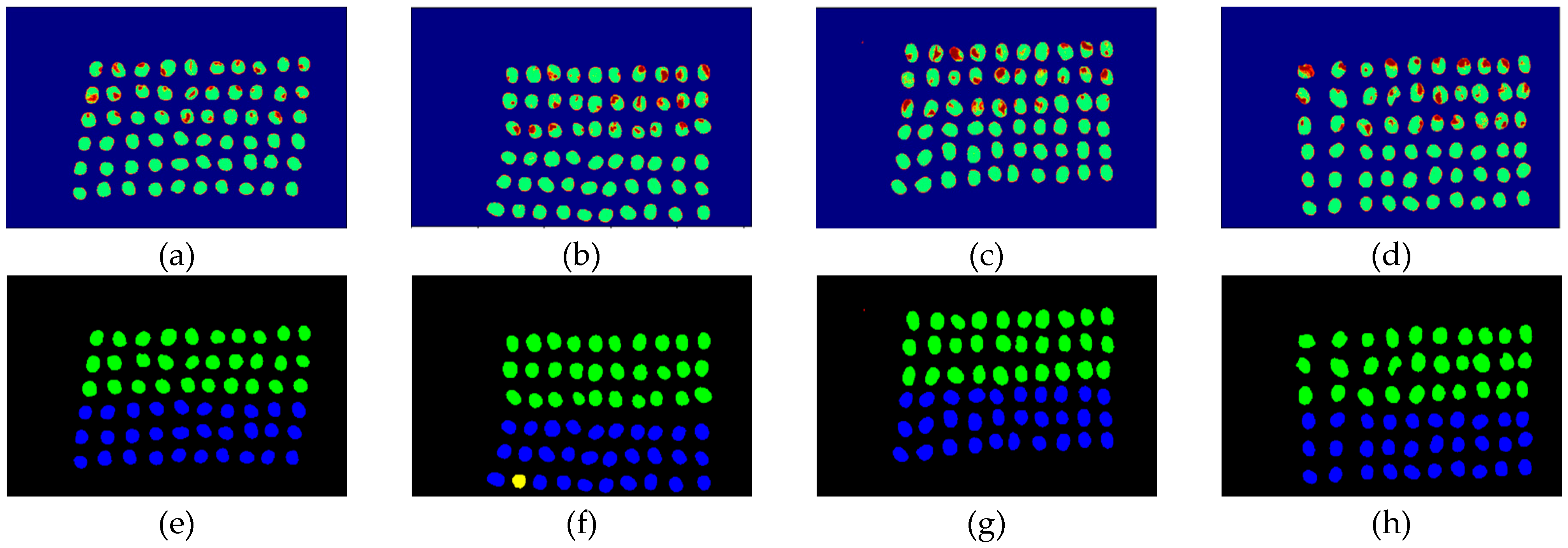
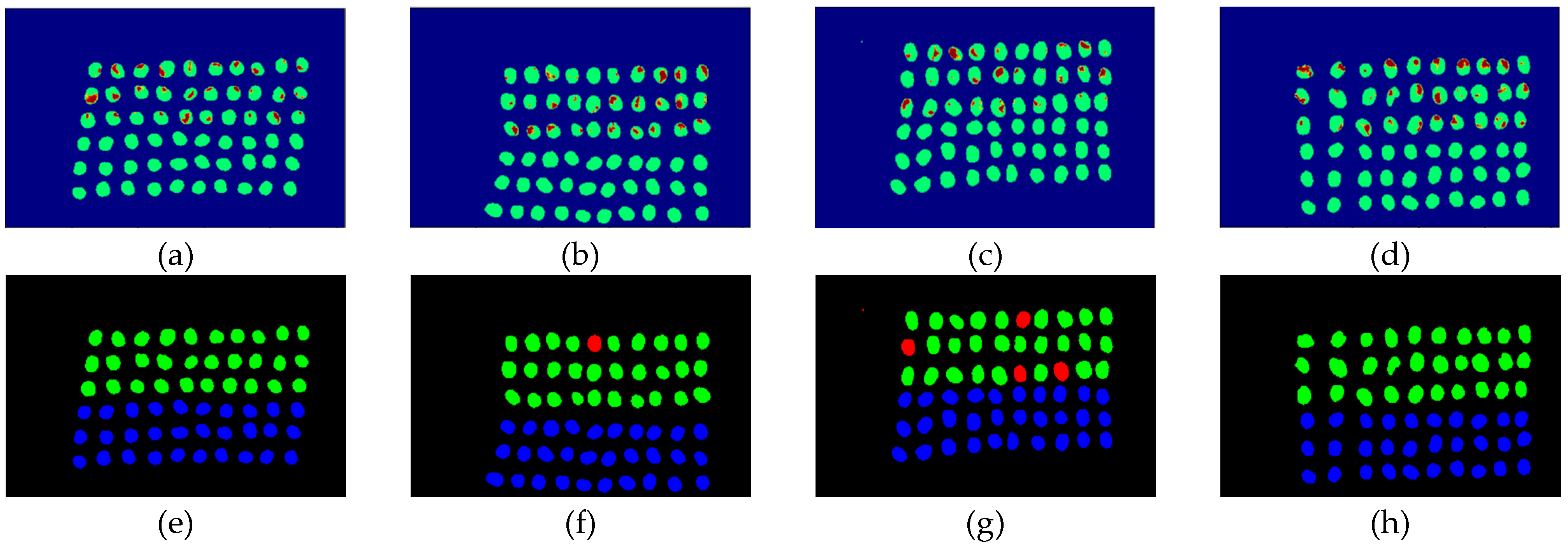
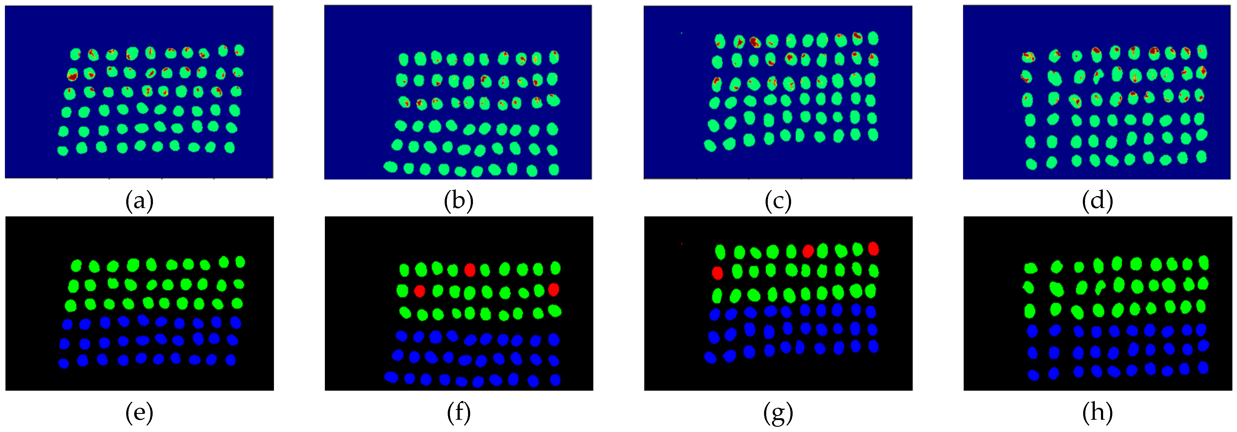
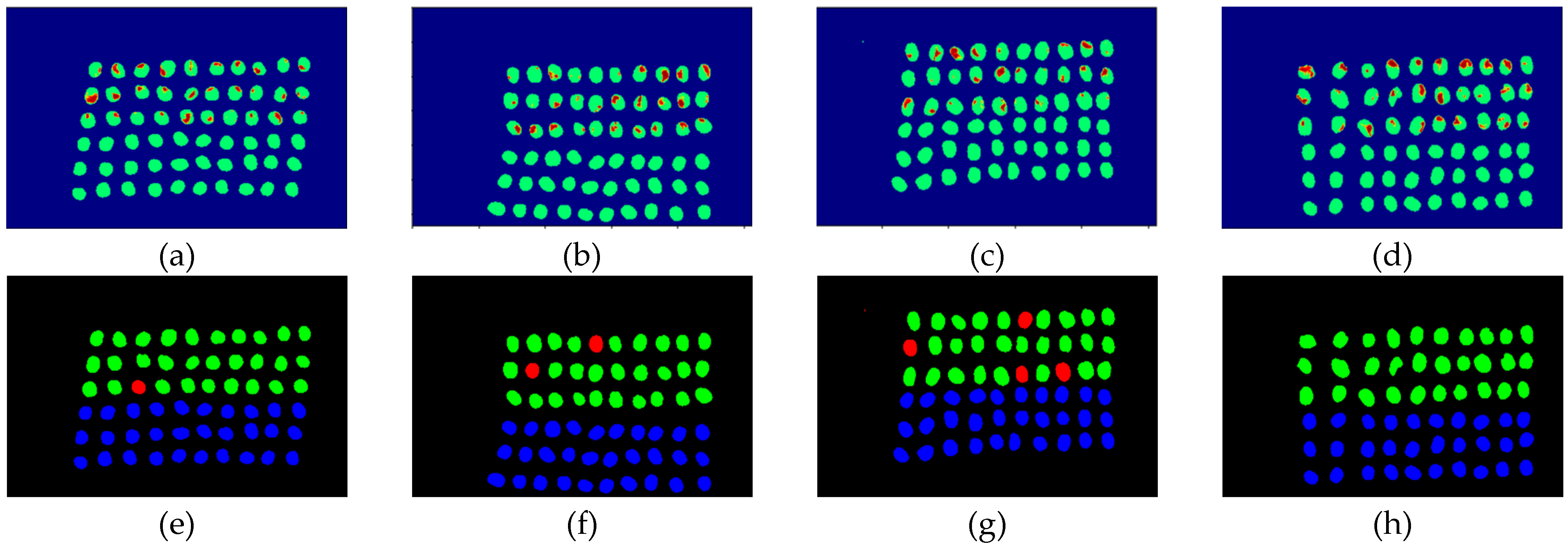
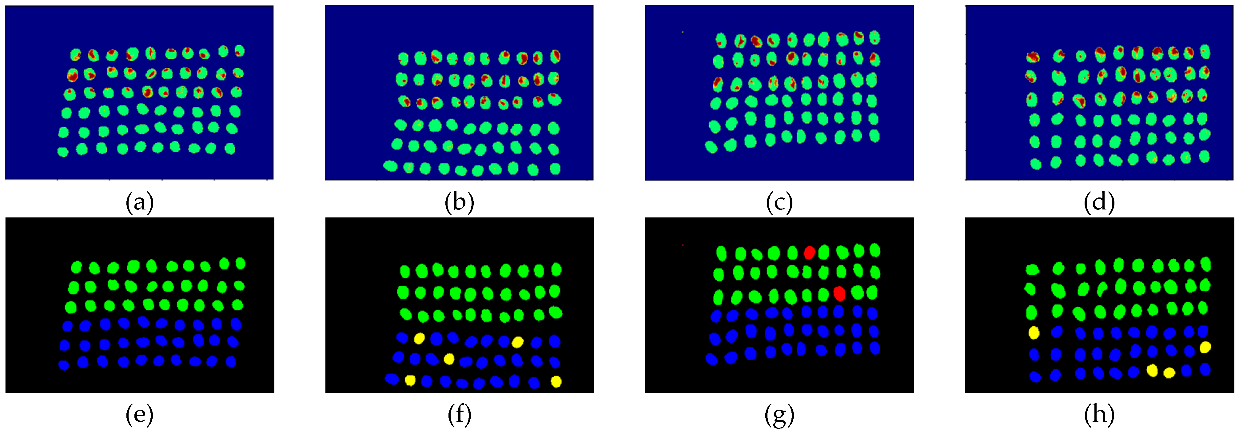
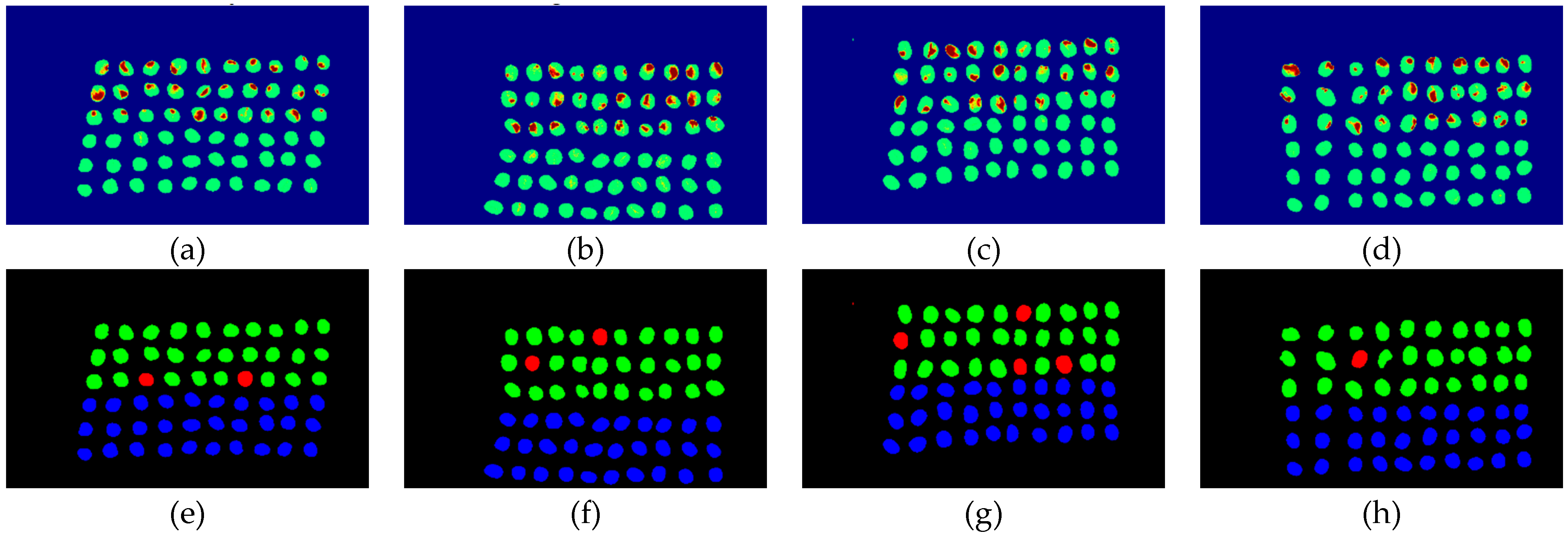
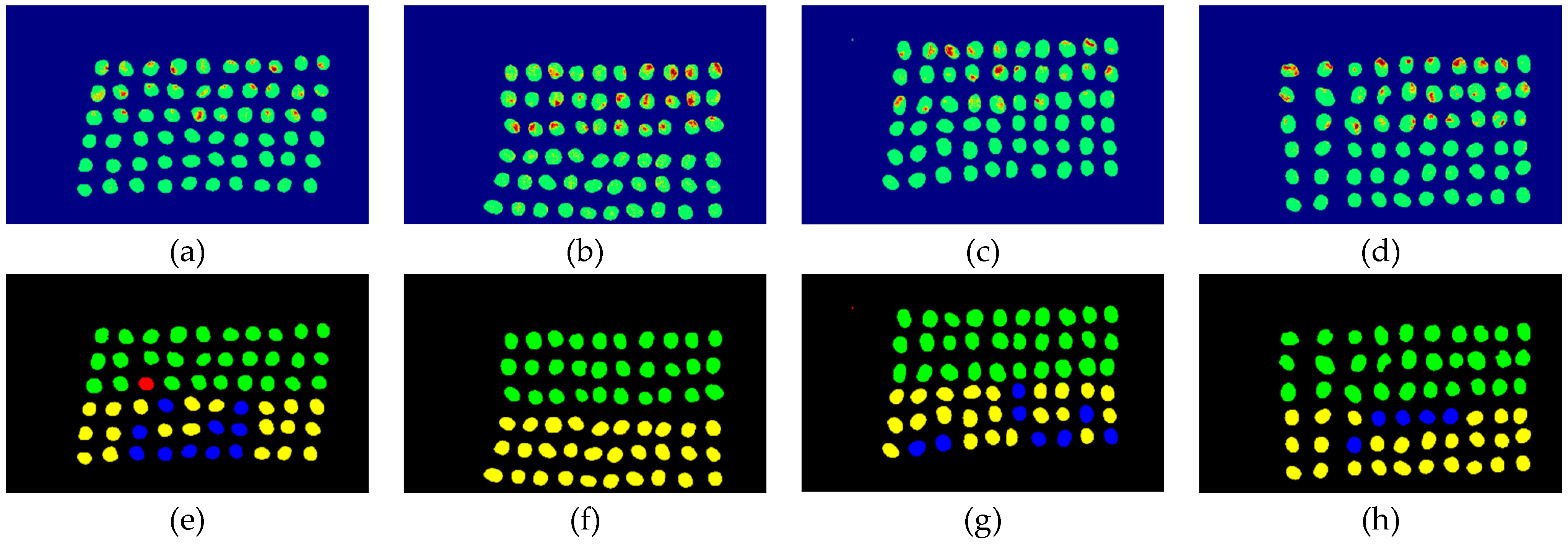
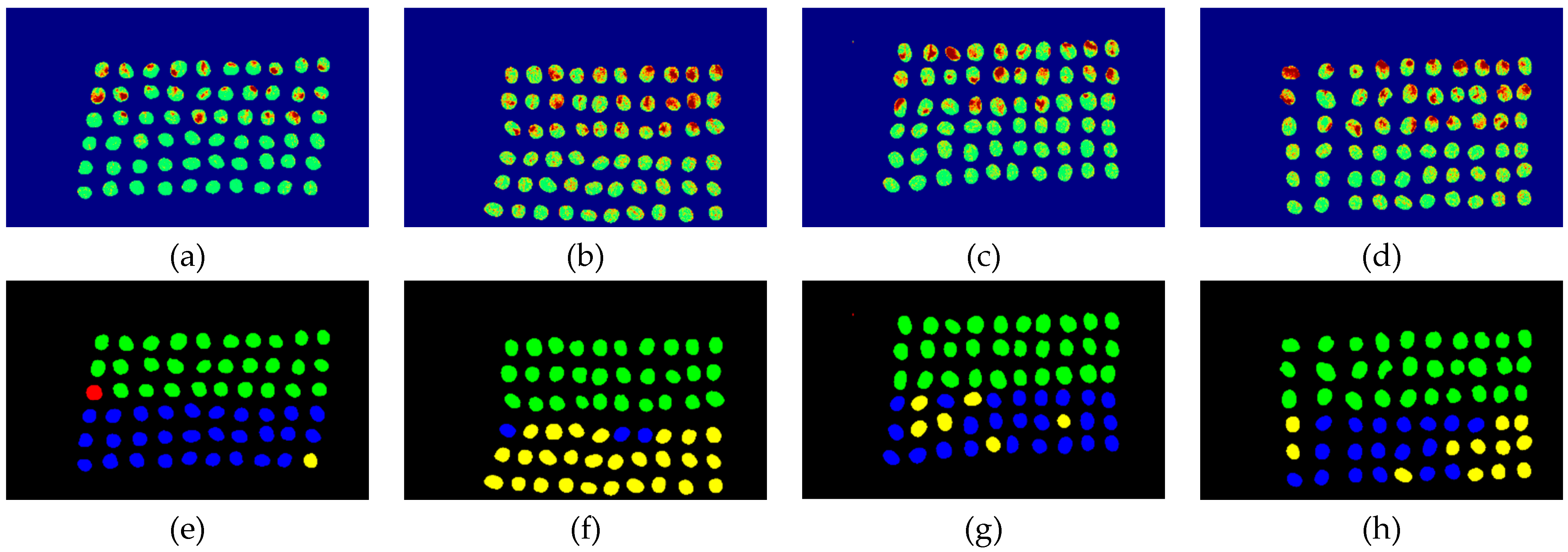
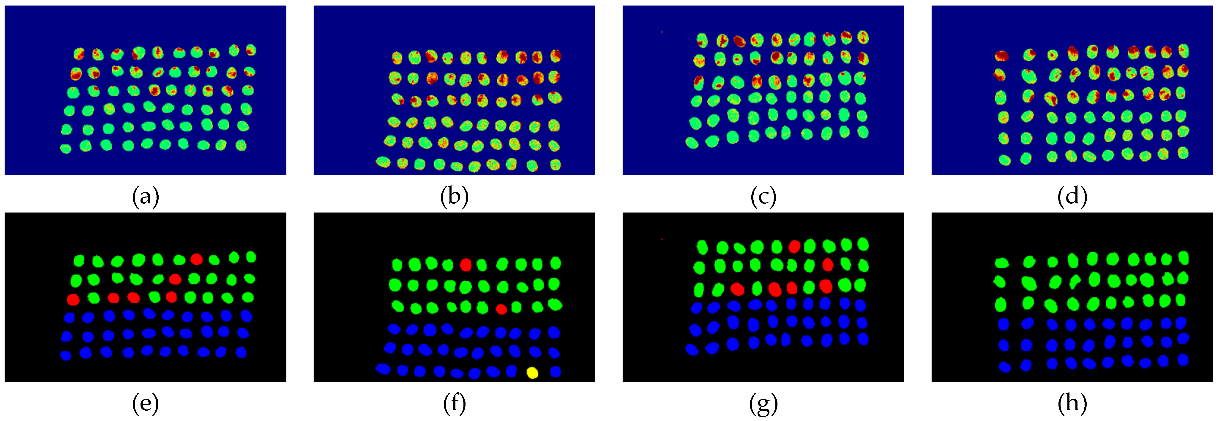
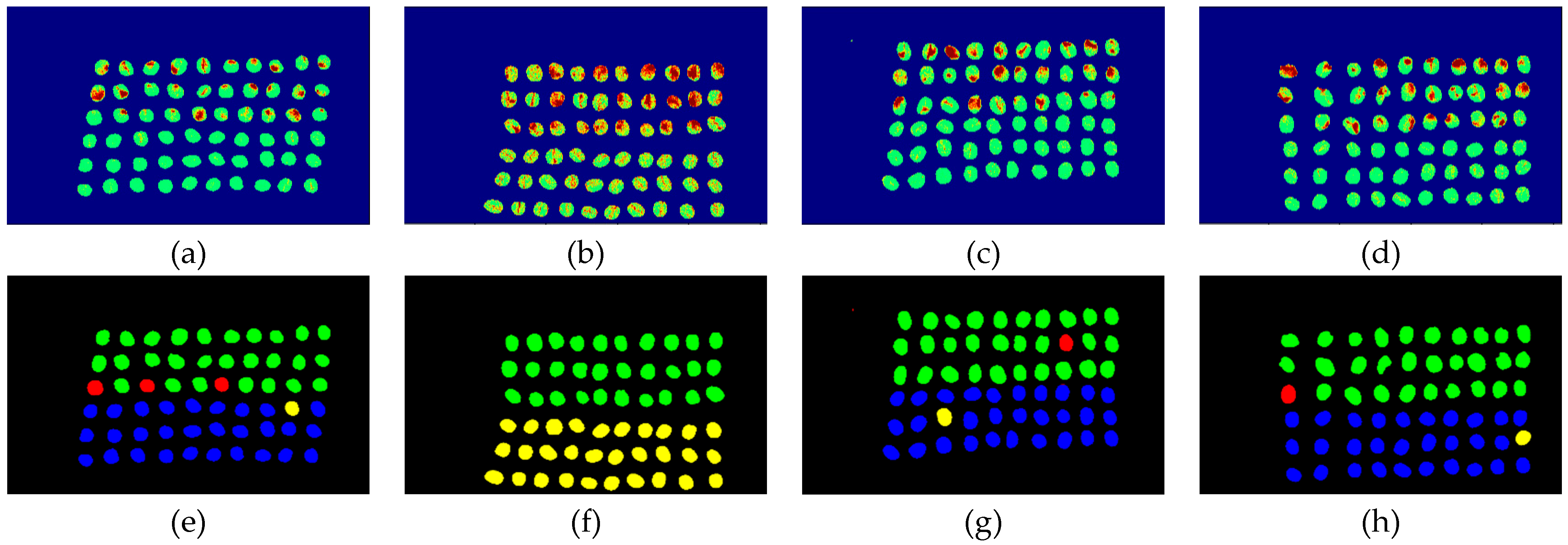
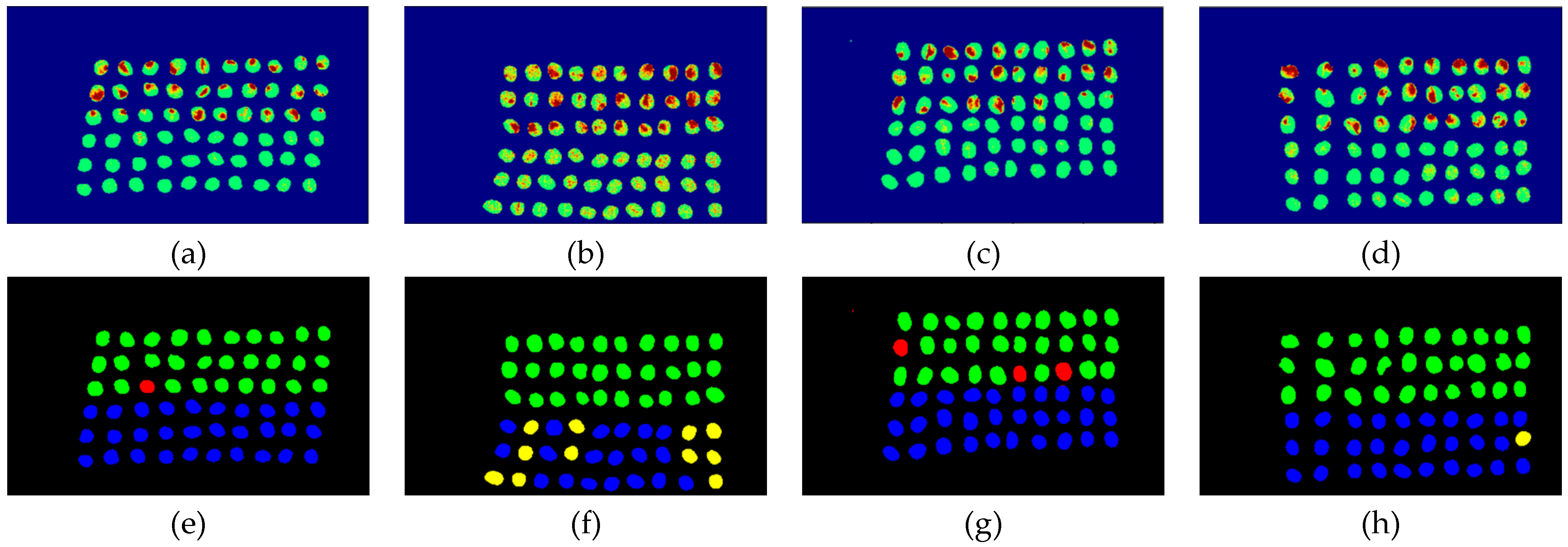
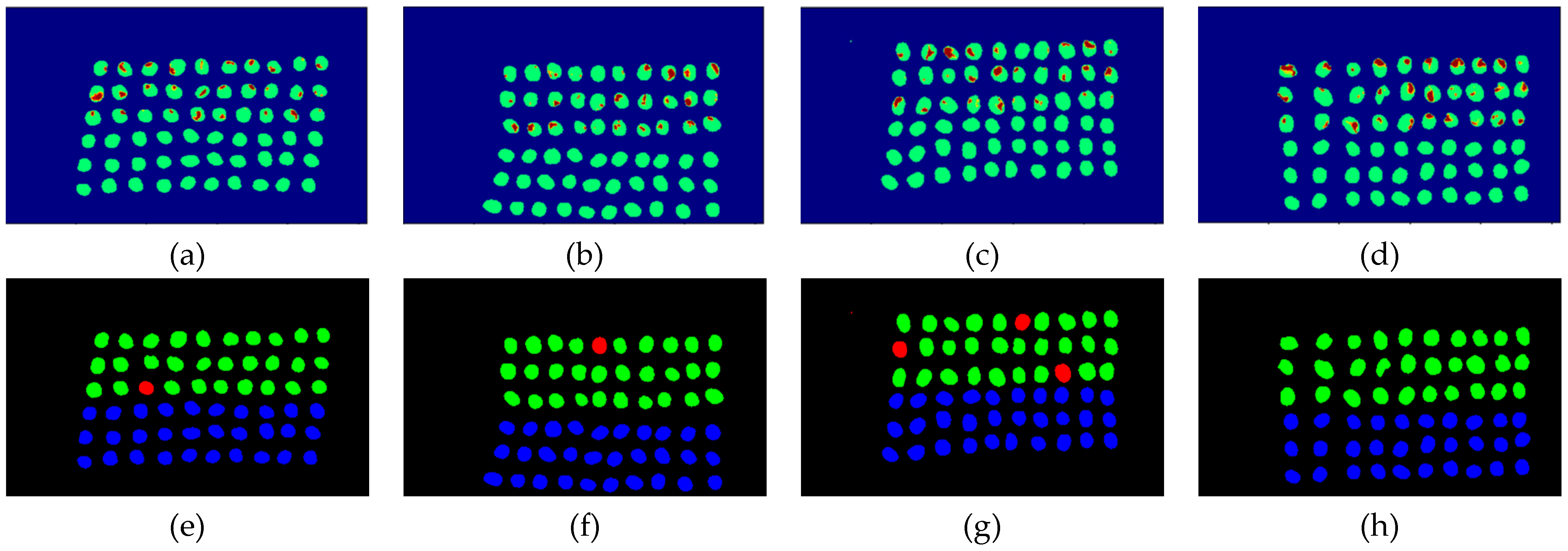
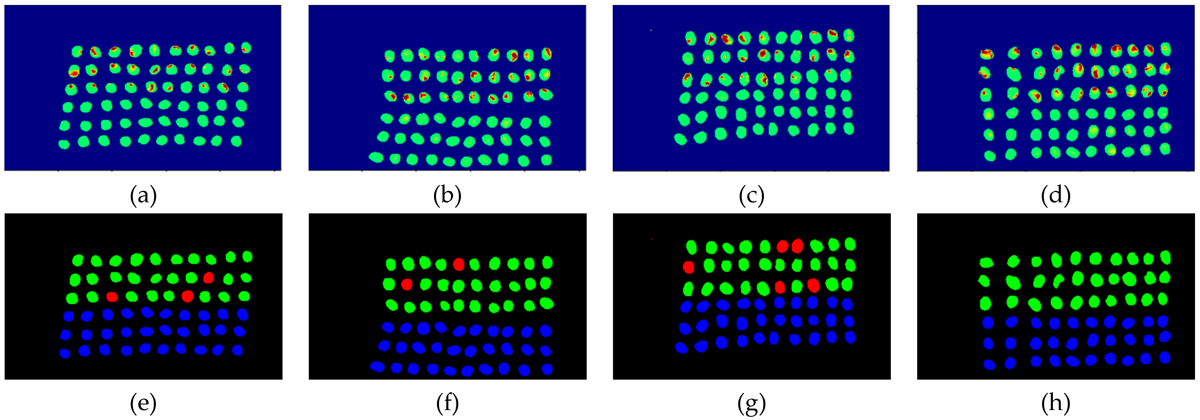
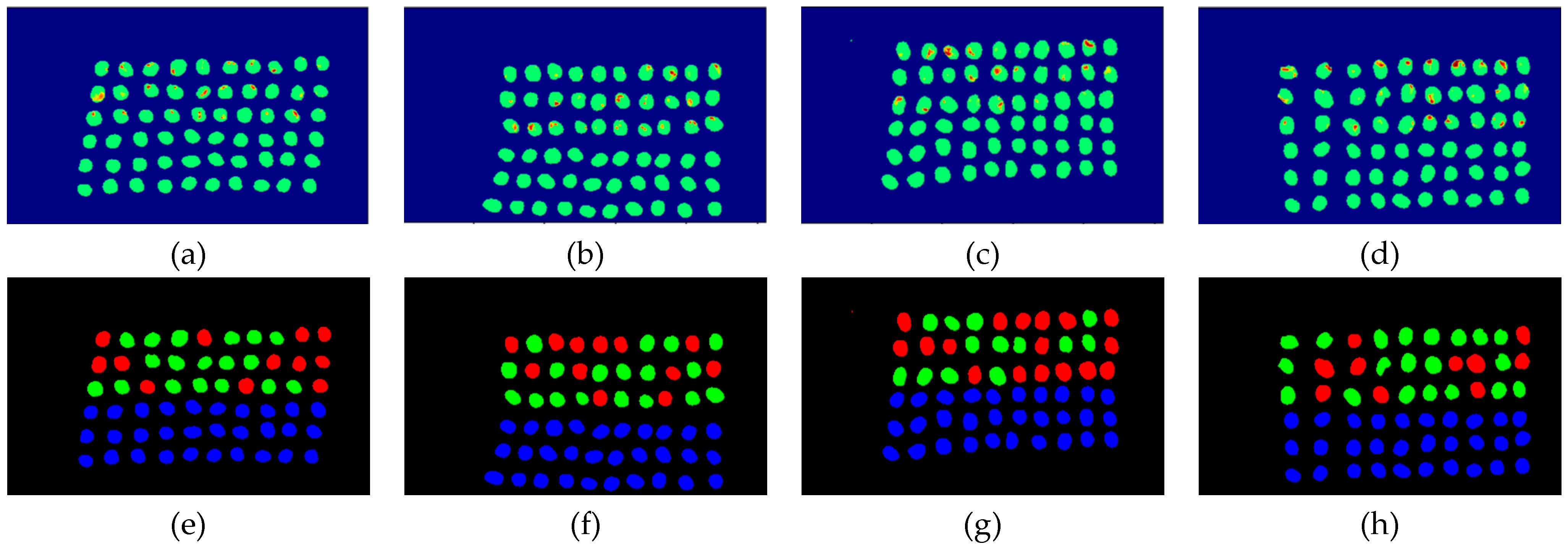
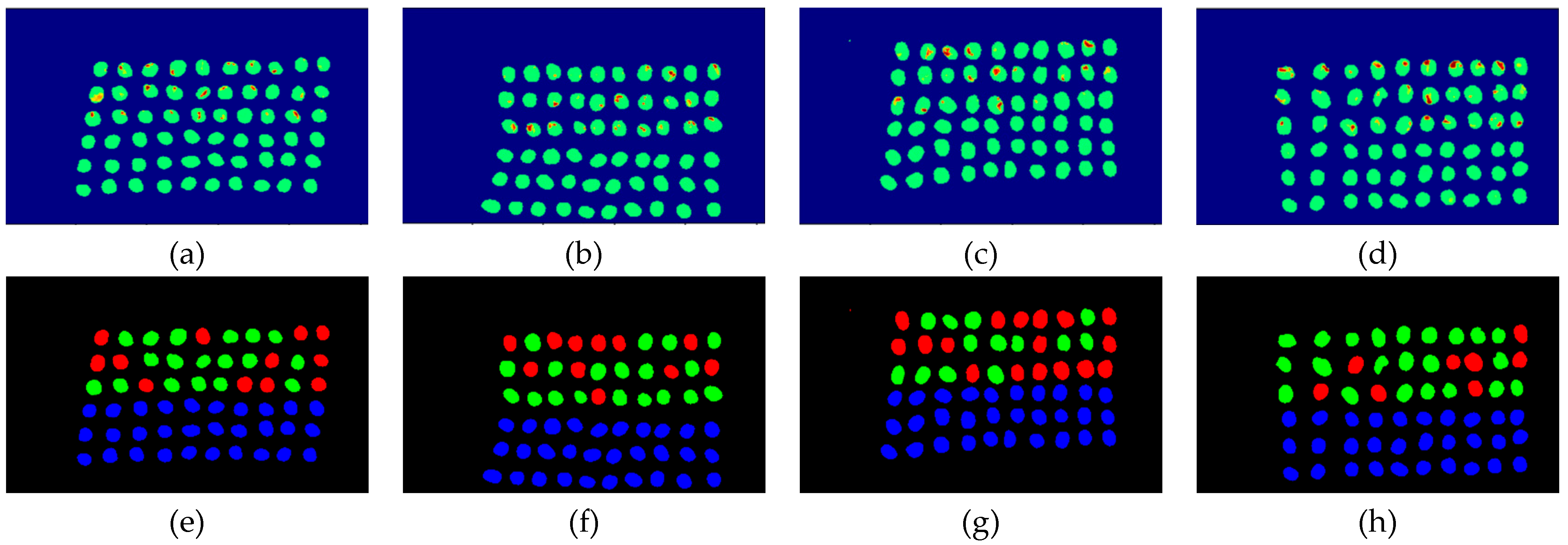
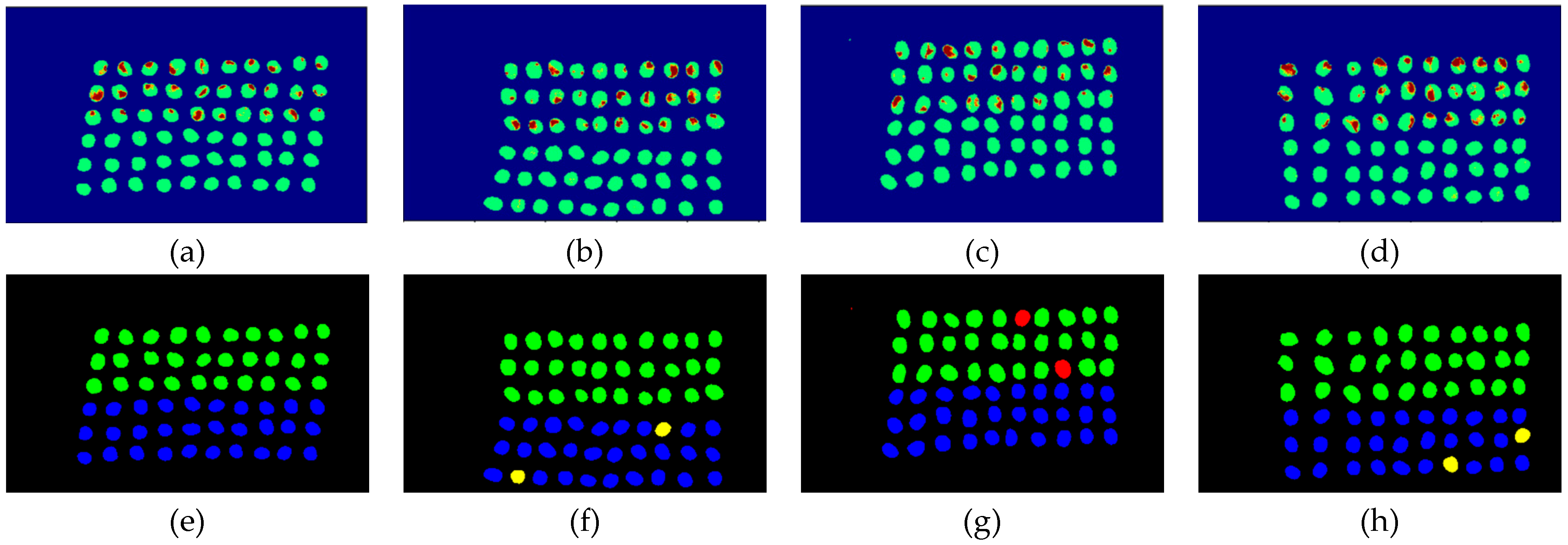
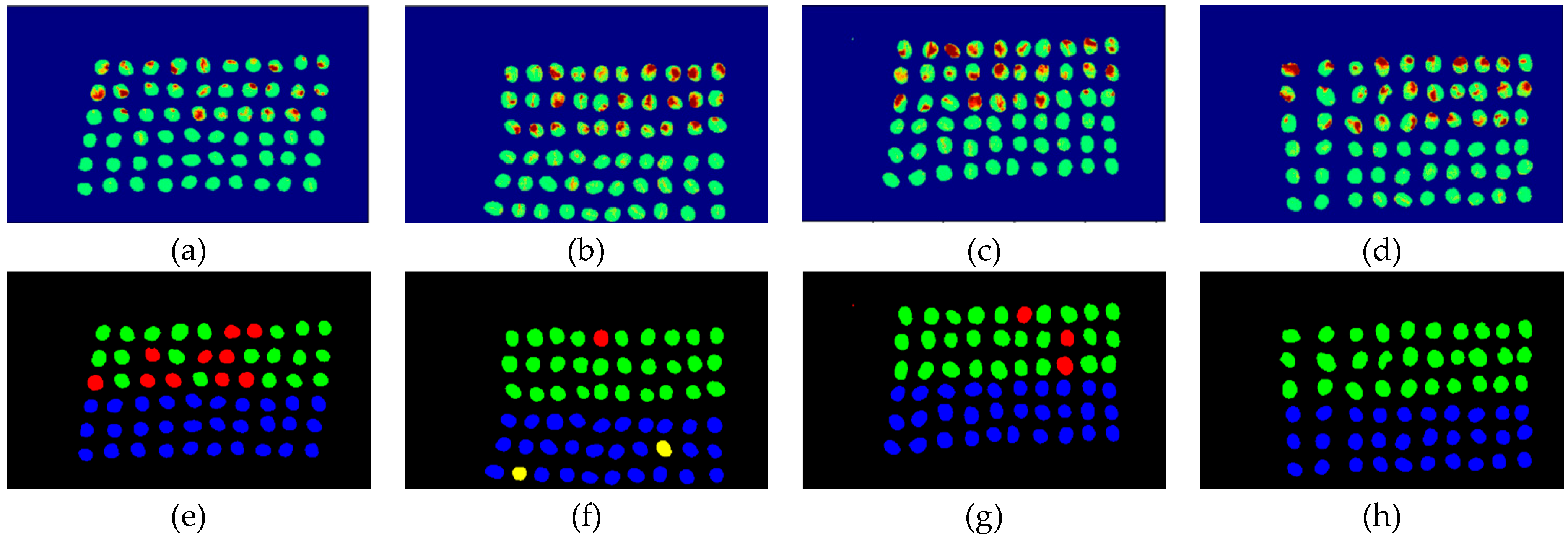
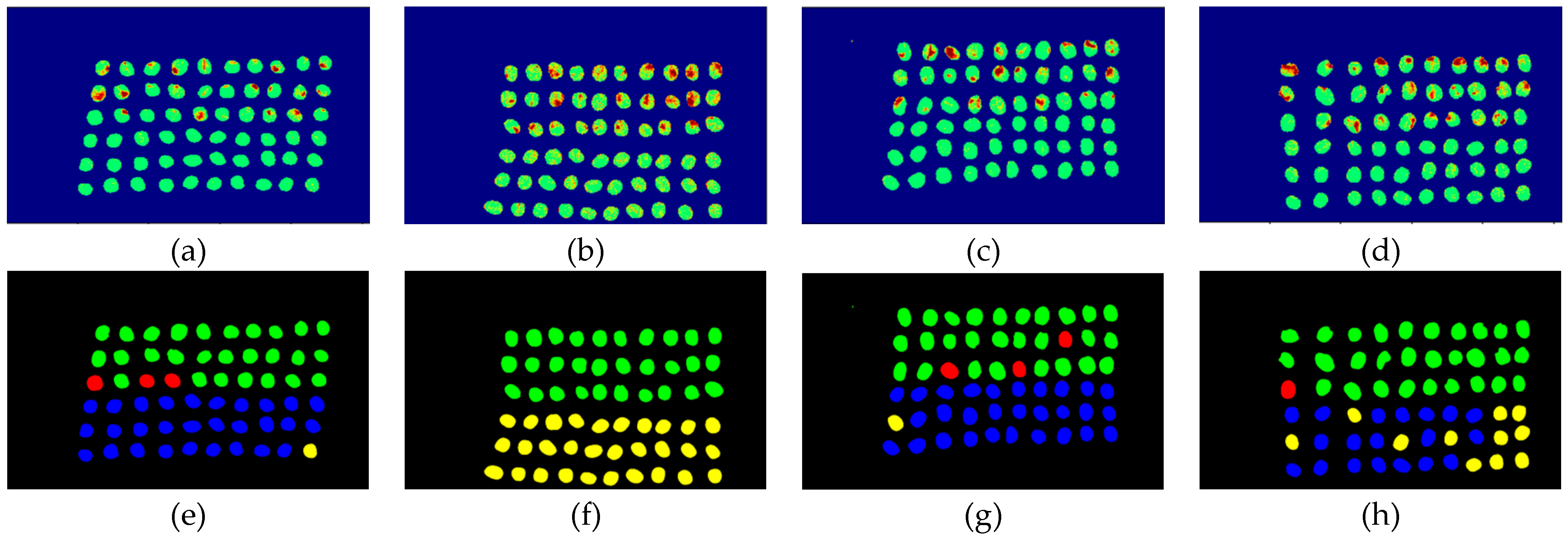
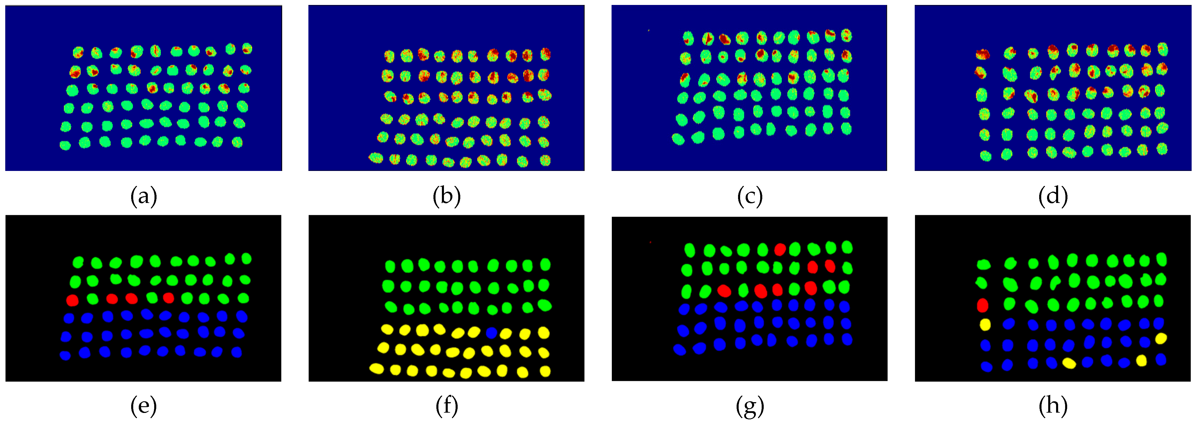
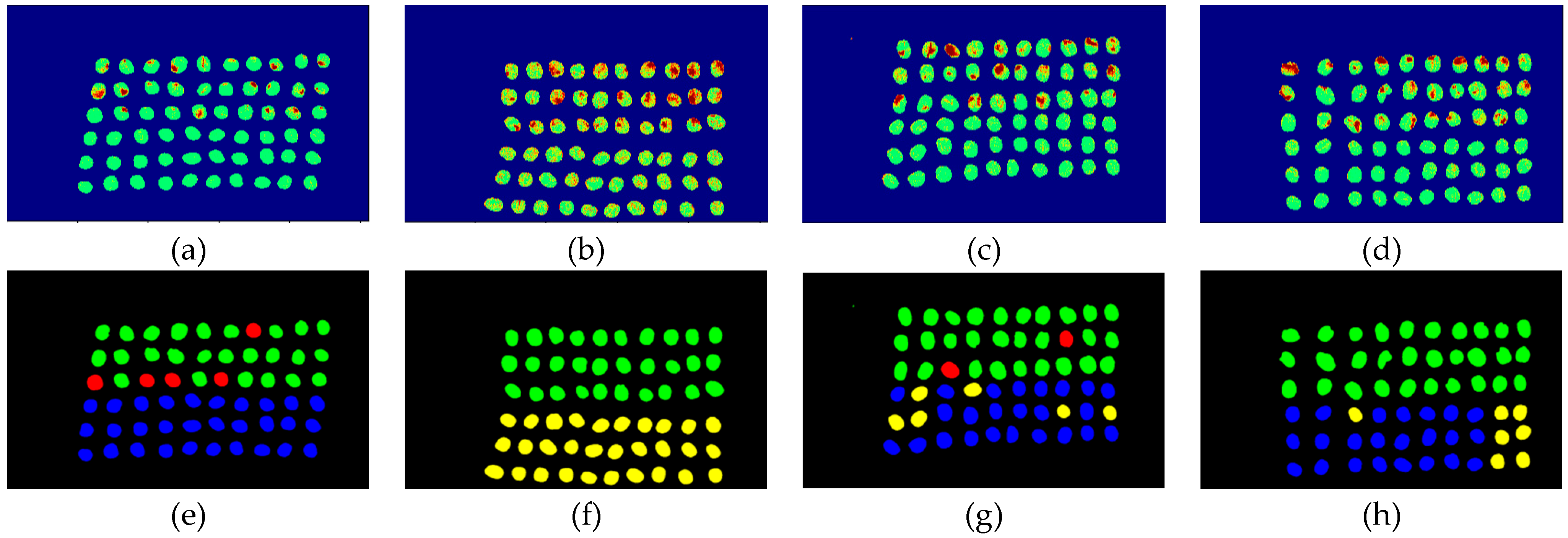
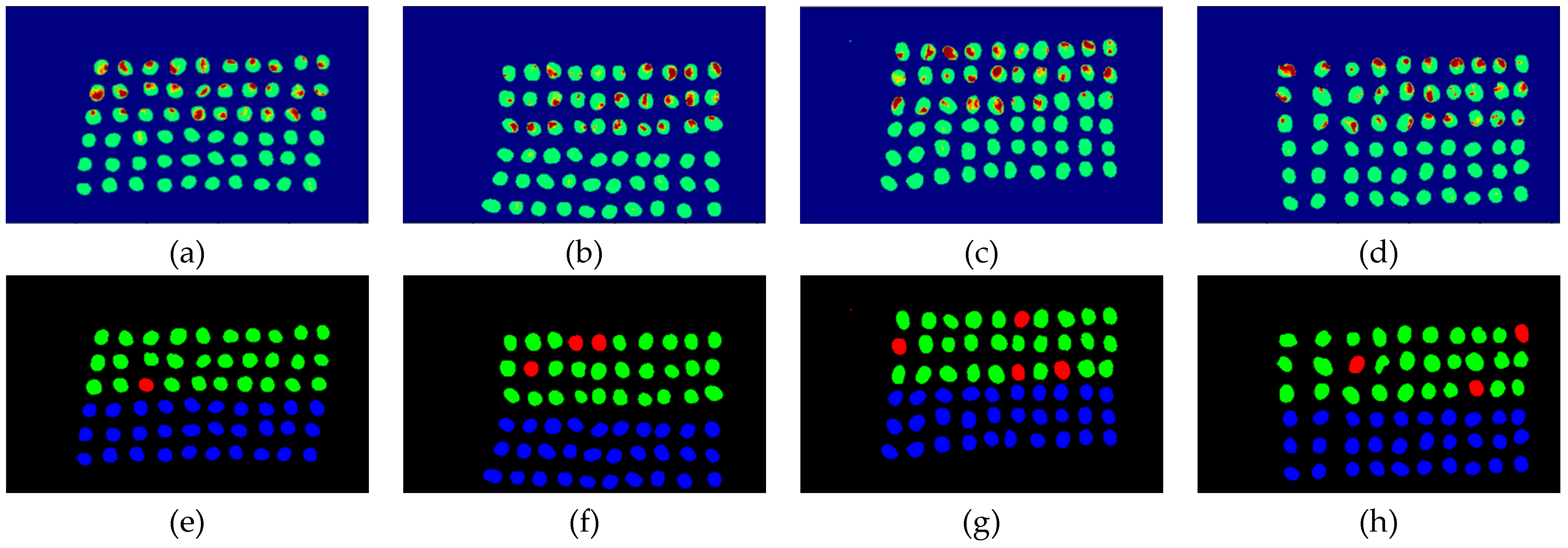
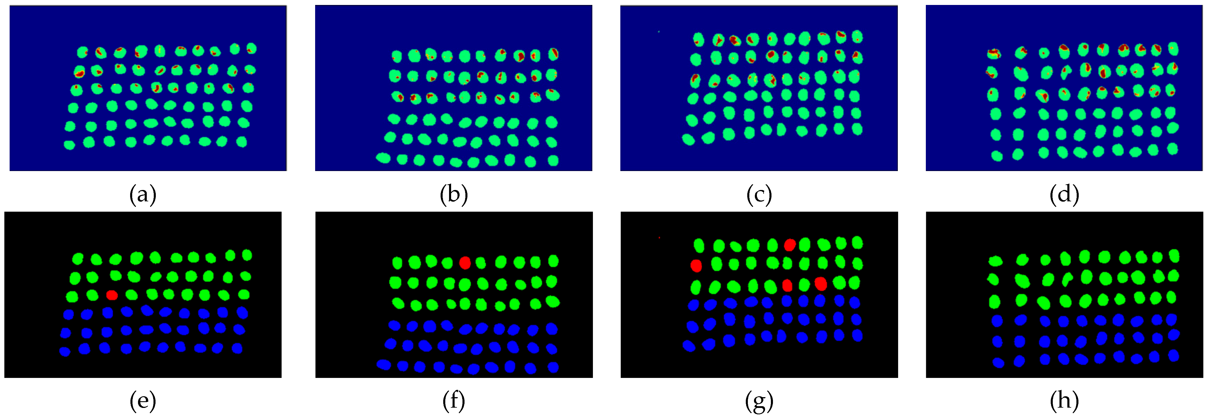
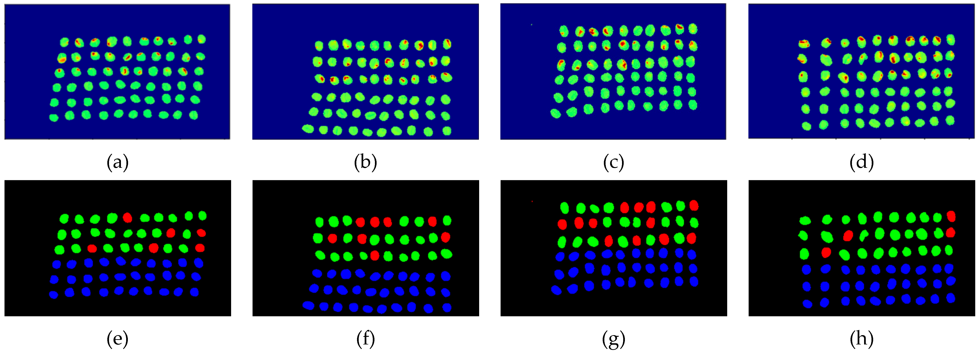
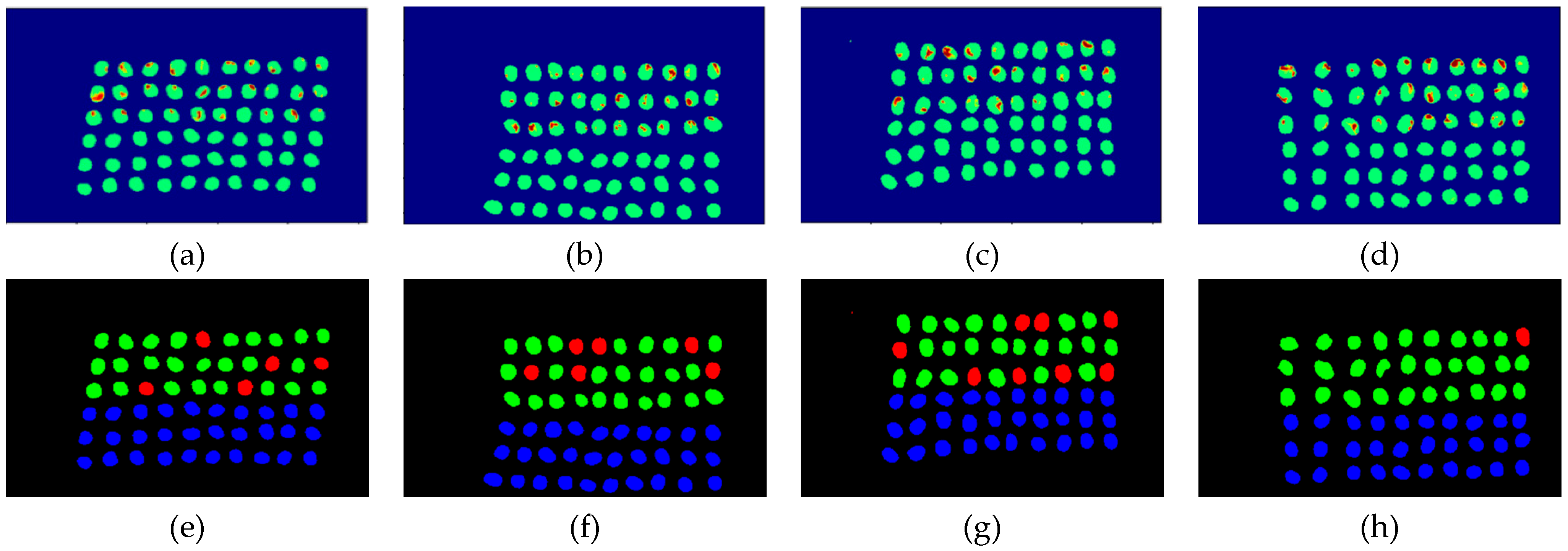
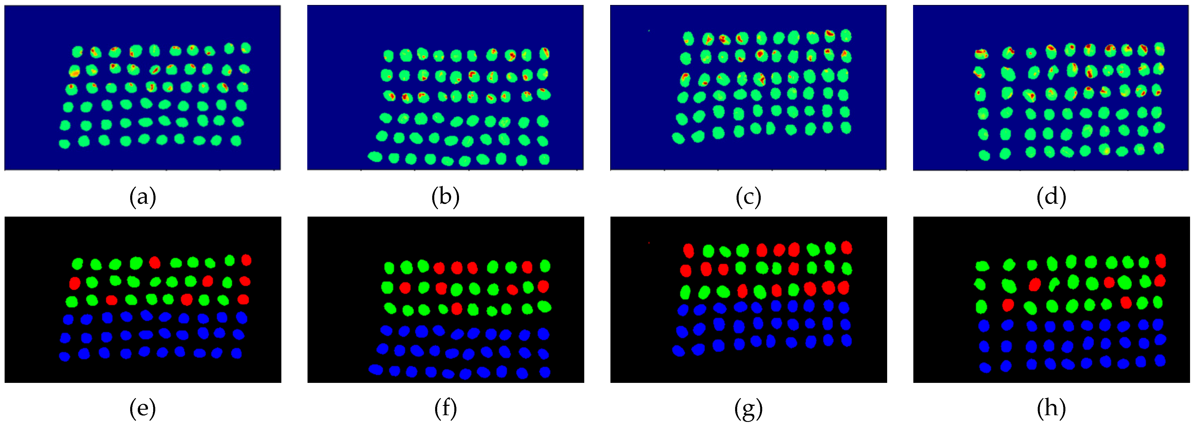
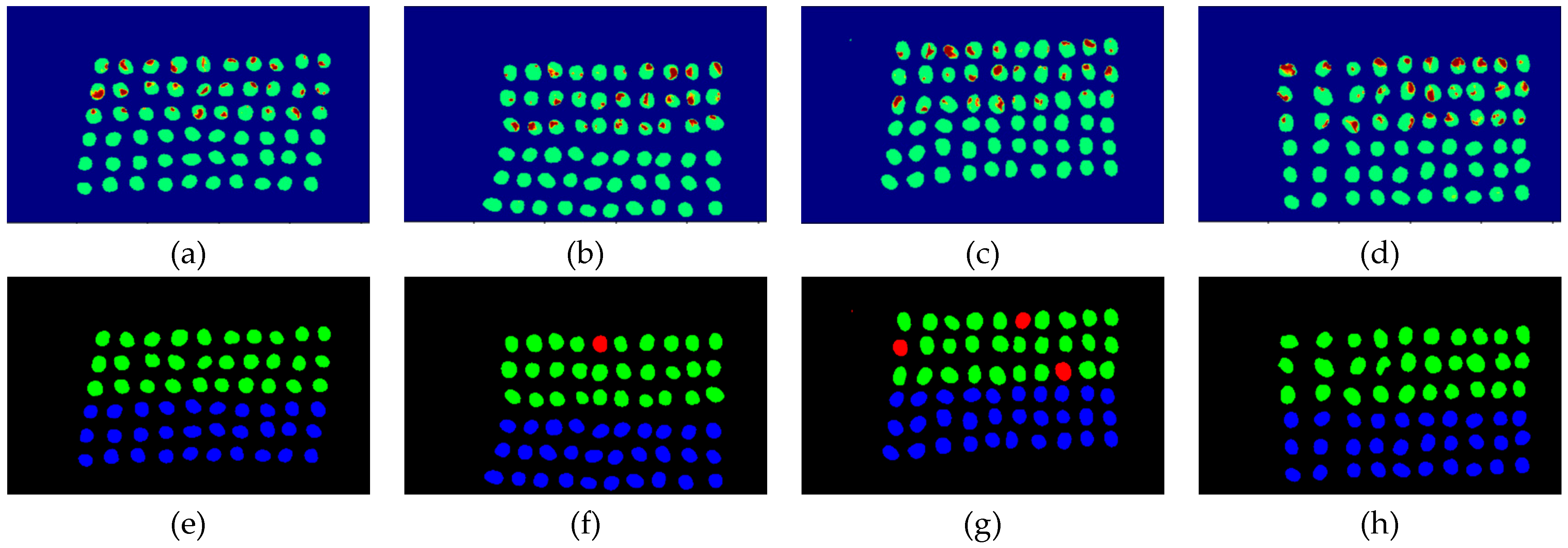
The final detection results using 10 bands were obtained by the CEM-SVM and the CNN model, as described in Section 2.3.7. Figure 16, Figure 17, Figure 18, Figure 19, Figure 20 and Figure 21 show the final detection results as generated by CEM-SVM using six band selection methods to select 10 bands, while Figure 22, Figure 23, Figure 24, Figure 25 and Figure 26 show the final detection results as obtained by the CNN model using five-band selection methods to select 10 bands. The upper three rows in Figure 16, Figure 17, Figure 18, Figure 19, Figure 20 and Figure 21 are insect damaged beans, while the lower three rows are healthy beans, and there were 1139 beans in 20 images. To limit the text length, only four of the 20 images are displayed, and the analysis results are shown in Table 3. In the confusion matrix of this experiment, TP refers to insect damaged bean hits, FN refers to missing insect damaged beans, TN refers to healthy bean hits, and FP refers to false alarms. In image representation, TP is green, FN is red, TN is blue, and FP is yellow; these colors are used for visualization, as shown in Figure 16, Figure 17, Figure 18, Figure 19, Figure 20, Figure 21, Figure 22, Figure 23, Figure 24, Figure 25 and Figure 26. All results of the three bands are compiled and compared in

Table 4. The results of the green coffee bean classification. The best performance is highlighted in red color.

3 Bands Green Coffee Beans CEM-SVM Results
Analysis Method	TP	FN	FP	TN	TPR	FPR	ACC	Kappa	Time (s)
CEM_BDM + CEM-SVM	520	50	17	552	0.912	0.298	0.941	0.887	11.57
MinV_BP + CEM-SVM	570	0	569	0	1.0	1.0	0.5	0	13.27
MaxV_BP + CEM-SVM	515	55	8	561	0.903	0.014	0.944	0.892	12.31
SF_CTBS + CEM-SVM	494	76	5	564	0.867	0.008	0.928	0.862	13.21
SB_CTBS + CEM-SVM	515	55	8	561	0.903	0.014	0.944	0.892	13.26
PCA + CEM-SVM	523	47	14	555	0.917	0.024	0.946	0.896	12.83
3 Bands Green Coffee Beans CNN Results
Analysis Method	TP	FN	FP	TN	TPR	FPR	ACC	Kappa	Time (s)
CEM_BDM + CNN	532	38	20	549	0.931	0.029	0.95	0.901	7.4
MaxV_BP + CNN	520	50	13	556	0.912	0.018	0.947	0.894	7.4
SF_CTBS + CNN	461	109	8	561	0.8	0.009	0.895	0.79	7.13
SB_CTBS + CNN	514	56	9	560	0.9	0.014	0.942	0.885	7.67
PCA + CNN	540	30	41	528	0.946	0.063	0.941	0.883	7.64

. The ACC [40], Kappa [41,42], and running time calculated by the confusion matrix were used for evaluation. The running time of this experiment was the average time.

In the case of three bands, CEM-SVM, BDM, MaxV_BP, SF_CTBS, SB_CTBS, and PCA were successful in classification. However, a portion of insect damaged beans was not detected, which was probably because the insect damage surface was not irradiated. The MinV_BP+CEM-SVM could not perform classification at all, as shown in Figure 17, possibly due to the non-selection of the sensitive band; thus, its result was excluded from subsequent discussion. As shown in Table 4, the PCA+CNN had the highest TPR, and PCA+CEM-SVM had the highest ACC and kappa, proving that the sequencing of the PCA amount of variation is feasible for band selection. The minimum FDR was observed for SF_CTBS+CEM-SVM. The minimum variance of CEM was used for recurrent selection in SF_CTBS, and the healthy beans could be identified accurately.

In the case of CNN, the BDM, MaxV_BP, SF_CTBS, SB_CTBS, and PCA were used, and the MinV_BP was not used because the deep learning label produced in CEM could not be identified. Here, the paper of three bands was not included for comparison. The PCA exhibited the highest TPR, and thus, the band selected by PCA was more sensitive to defective beans. The SF_CTBS had the lowest FPR, and the minimum variance of CEM calculated by SF_CTBS for recurrent selection could accurately identify healthy beans. The classification result indicates that only eight green coffee beans were misidentified as defective beans, CEM_BDM possessed the highest ACC and kappa, and that the CEM_BDM method classified green coffee beans better. In terms of time, the CNN was faster than SVM because the CNN model used a batch_size = 1024 for prediction, while the SVM used pixels one by one for prediction.

3.3. Detection Results Using 10 Bands

The final detection results using 10 bands were obtained by CEM-SVM and the CNN model, as described in Section 2.3.7. Figure 27, Figure 28, Figure 29, Figure 30, Figure 31 and Figure 32 show the final detection results, as generated by CEM-SVM using six band selection methods to select 10 bands; Figure 33, Figure 34, Figure 35, Figure 36 and Figure 37 show the final detection results as obtained by the CNN model using five-band selection methods to select 10 bands.

All results from the 10 bands were compiled and compared, as shown in

Table 5. The results of the green coffee bean classification. The best performance is highlighted in red color.

10 Bands Green Coffee Beans SVM Results
Analysis Method	TP	FN	FP	TN	TPR	FPR	ACC	Kappa	Time (s)
CEM_BDM+CEM-SVM	509	61	8	561	0.892	0.014	0.939	0.883	11.71
MinV_BP+CEM-SVM	565	5	492	77	0.991	0.864	0.563	0.131	11.35
MaxV_BP+CEM-SVM	554	16	213	356	0.971	0.374	0.798	0.592	11.47
SF_CTBS+CEM-SVM	505	65	37	532	0.885	0.065	0.910	0.824	11.31
SB_CTBS+CEM-SVM	545	25	146	423	0.956	0.256	0.849	0.696	11.44
PCA+CEM-SVM	541	29	63	506	0.949	0.110	0.919	0.844	11.40
10 Bands Green Coffee Beans SVM Results
Analysis Method	TP	FN	FP	TN	TPR	FPR	ACC	Kappa	Time (s)
CEM_BDM+CNN	484	86	5	564	0.85	0.007	0.921	0.842	7.16
MaxV_BP+CNN	473	97	2	567	0.833	0.003	0.914	0.829	7.34
SF_CTBS+CNN	246	324	1	568	0.420	0.001	0.708	0.418	6.98
SB_CTBS+CNN	289	281	1	568	0.5	0.001	0.748	0.497	7.41
PCA+CNN	532	38	21	548	0.931	0.033	0.949	0.898	7.41

. As seen, there were several influential bands in the front, but excessive bands could induce misrecognitions.

In the case of CEM-SVM, the CEM_BDM+CEM-SVM had the best performance in FPR, ACC, and kappa, indicating the reliability of the CEM_BDM band priority in 10 bands, and the minimization of correlation between bands could influence green coffee beans. The sensitive bands were extracted using this method. The MaxV_BP+CEM-SVM had the highest TPR, indicating that the maximum variance of CEM calculated by MaxV_BP for sequencing could classify defective beans. The MinV_BP was less effective than the other methods, which might be related to the variance of green coffee beans, suggesting that this method is inapplicable to a small number of bands.

In the case of CNN, when the MinV_BP produced labels, excessive data misrecognitions failed the training model, and the PCA had the highest TPR, ACC, and Kappa. Therefore, in the bands selected from the 10 bands, the PCA+CNN seemed to be the most suitable for classifying green coffee beans. The SF_CTBS and SB_CTBS had the minimum FPR, indicating that the cyclic ordering of CEM variance is appropriate for classifying good beans.

3.4. Detection Results by Using 20 Bands

The final detection results using 20 bands were obtained by the CEM-SVM and the CNN model, as described in Section 2.3.7. Figure 38, Figure 39, Figure 40, Figure 41, Figure 42 and Figure 43 show the final detection results, as generated by CEM-SVM using six band selection methods to select 10 bands; Figure 44, Figure 45, Figure 46, Figure 47 and Figure 48 show the final detection results as obtained by the CNN model using five-band selection methods to select 10 bands.

All results of the 20 bands were compiled and compared, as shown in

Table 6. The results of the green coffee bean classification. The best performance is highlighted in red color.

20 Bands Green Coffee Beans SVM Results
Analysis Method	TP	FN	FP	TN	TPR	FPR	ACC	Kappa	Time (s)
CEM_BDM+CEM-SVM	522	48	21	548	0.915	0.036	0.939	0.881	12.03
MinV_BP+CEM-SVM	547	23	77	492	0.959	0.135	0.912	0.827	11.34
MaxV_BP+CEM-SVM	550	20	249	320	0.964	0.437	0.763	0.525	11.41
SF_CTBS+CEM-SVM	521	49	135	434	0.914	0.237	0.838	0.681	11.38
SB_CTBS+CEM-SVM	544	26	253	316	0.954	0.444	0.755	0.516	11.78
PCA+CEM-SVM	546	24	144	425	0.957	0.253	0.852	0.729	11.38
20 Bands Green Coffee Beans CNN Results
Analysis Method	TP	FN	FP	TN	TPR	FPR	ACC	Kappa	Time (s)
CEM_BDM+CNN	480	90	5	564	0.842	0.007	0.917	0.835	7.84
MaxV_BP+CNN	355	215	1	568	0.62	0.001	0.809	0.618	7.27
SF_CTBS+CNN	395	175	2	567	0.687	0.003	0.841	0.683	7.35
SB_CTBS+CNN	336	234	1	568	0.585	0.001	0.791	0.583	7.13
PCA+CNN	511	59	5	564	0.896	0.007	0.944	0.888	7.82

. The ACC, kappa, and the running time calculated by the confusion matrix were used for evaluation.

In the case of CEM-SVM, the CEM_BDM+CEM-SVM exhibited the best performance in FPR, ACC, and kappa, proving again that the minimization of inter-band correlation is helpful to the classification of green coffee beans. The MaxV_BP exhibited the highest TPR, and using the maximum variance of CEM for ordering, it could classify defective beans in 20 bands. It is noteworthy that the MinV_BP+CEM-SVM selected sensitive bands from 20 bands, which may be the variance calculation problem of the algorithm, proving that the MinV_BP method is inapplicable to a small number of bands of green coffee beans, but applicable to a larger number of bands.

In the case of CNN, as the data content increased, the accuracy of most methods declined. In the training of MinV_BP, excessive data misrecognition failed the training model. The PCA band selection exhibited good performance in TPR, ACC, and kappa, indicating that the PCA performed the best in classification with 20 bands. The MaxV_BP and SB_CTBS had the lowest FPR. The use of the maximum variance of CEM in the case of 20 bands had the best effect on classifying good beans.

3.5. Discussion

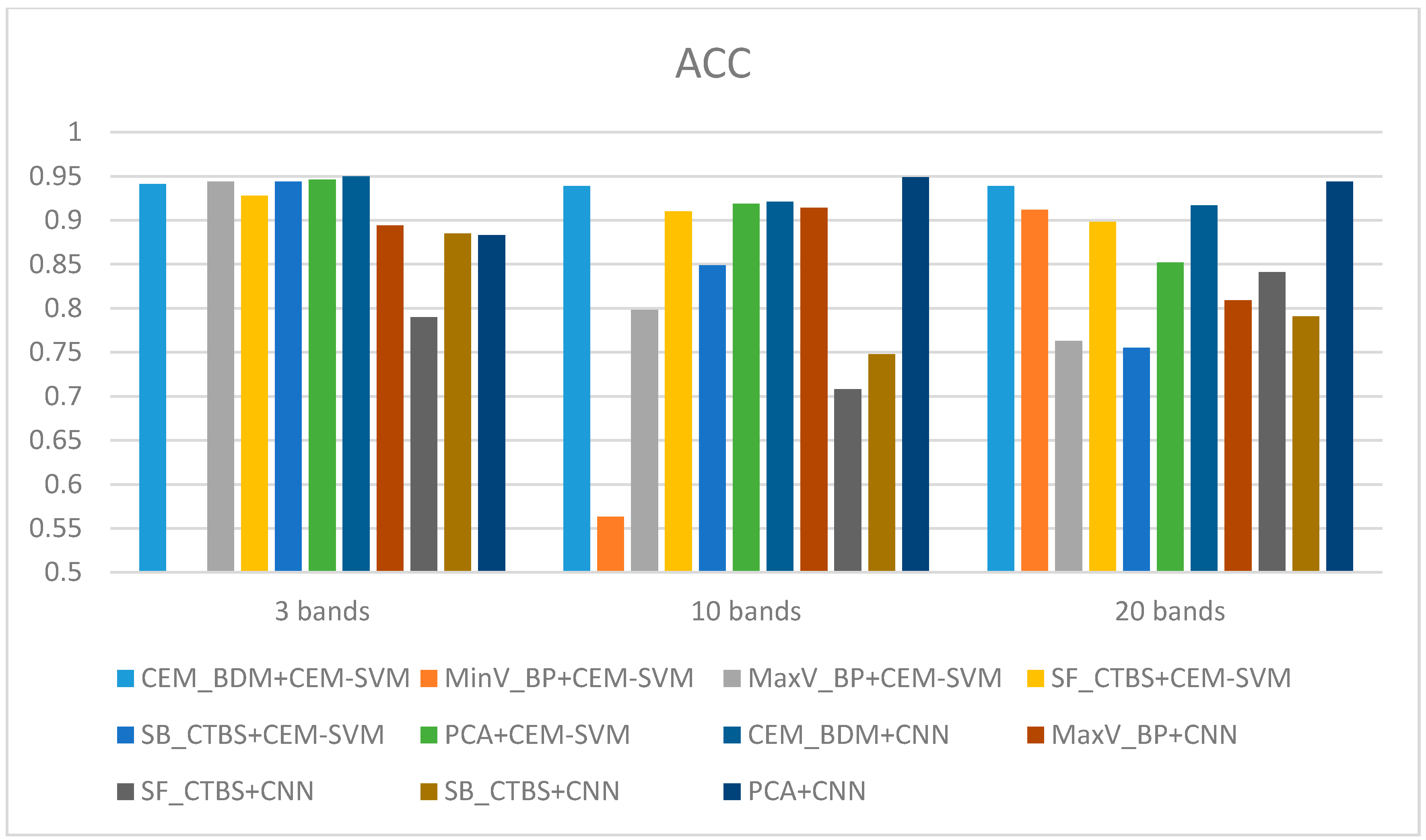
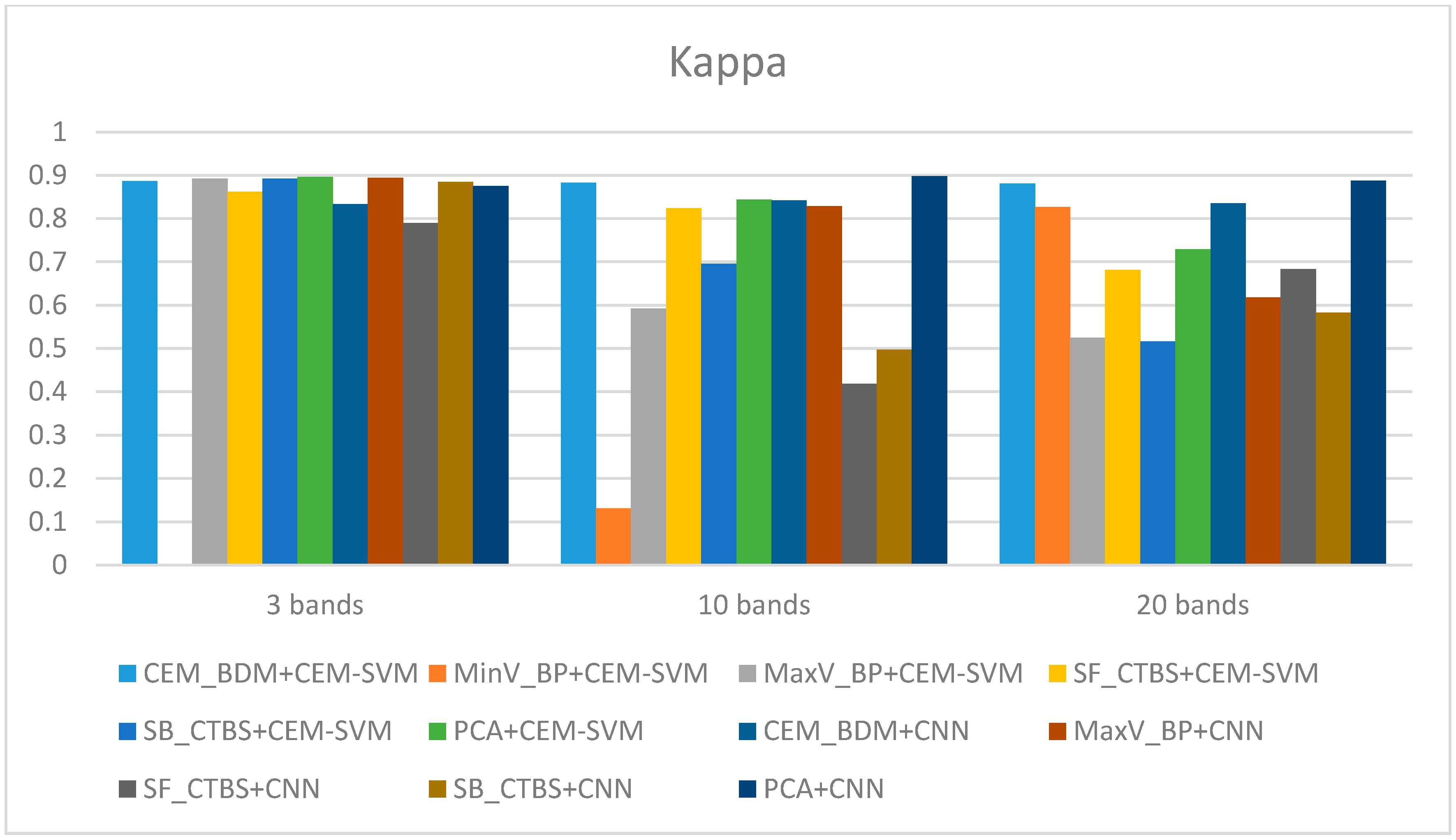
The ACC and kappa values of three bands, 10 bands, and 20 bands were compared and represented as histograms, as shown in Figure 49 and Figure 50. According to the comparison results of the figures, the CEM_BDM+CEM-SVM gave good results in the case of three bands, 10 bands, and 20 bands. The accuracy was higher than 90%, and the kappa was about 0.85, indicating that the BDM selected bands are crucial and representative to both classifiers for better performance. Considering MinV_BP+CEM-SVM in the cases of three bands and 10 bands, the selected bands might be difficult to classify the data, although there were sufficient data in the case of 20 bands, where the effect was enhanced greatly, suggesting that MinV_BP needs a larger number of bands for better classification.

As for MaxV_BP+CEM-SVM, the green coffee beans could be classified in the cases of three bands and 10 bands; but the accuracy declined in the case of 20 bands, indicating excessive bands induced misrecognitions. Interestingly, this situation is contrary to MinV_BP, and is related to the CEM variance of MinV_BP and MaxV_BP. When assessing SF_CTBS+CEM-SVM, in the cases of three bands and 10 bands, the accuracy and Kappa values were quite high, while in the case of 20 bands, there were too many misrecognitions of healthy beans, and the kappa decreased greatly. This indicates that excessive bands induced misrecognitions, and confirms that the sensitive bands were identified from the first 10 bands. Considering SB_CTBS+CEM-SVM, in the case of three bands, high precision and kappa were observed, and with the increase in the number of bands, the rate of healthy bean misrecognition increased. Therefore, the first three bands of this method were the most representative, and excessive bands did not increase the accuracy. When assessing PCA+CEM-SVM, in the cases of three bands, 10 bands, and 20 bands, the results were good, and the variation seemed feasible for band selection, about the same as previous BDM. The two methods could thus select important spectral signatures with a small number of bands. In the cases of three bands, 10 bands, and 20 bands, the CEM_BDM+CNN exhibited good results, but poorer than the previous SVM in the cases other than three bands.

In the case of three bands, MaxV_BP+CNN exhibited a high precision and kappa, which reduced as the bands increased, but CNN seemed to be more suitable than SVM. The SF_CTBS+CNN had a poorer effect than SVM in the cases of three bands, 10 bands, and 20 bands, indicating that this method is inapplicable to CNN, which may be related to the variance of CEM. The SB_CTBS+CNN exhibited high precision and kappa in the case of three bands, which reduced as the bands increased. This suggests that excessive bands influenced the decision, and there was no significant difference, except for a slight difference in the case of 10 bands from SVM. The PCA+CNN exhibited good results in the cases of three bands, 10 bands, and 20 bands; the CNN performed much better than SVM, where the results were quite average, and the cases of 10 bands and 20 bands exhibited the best effect.

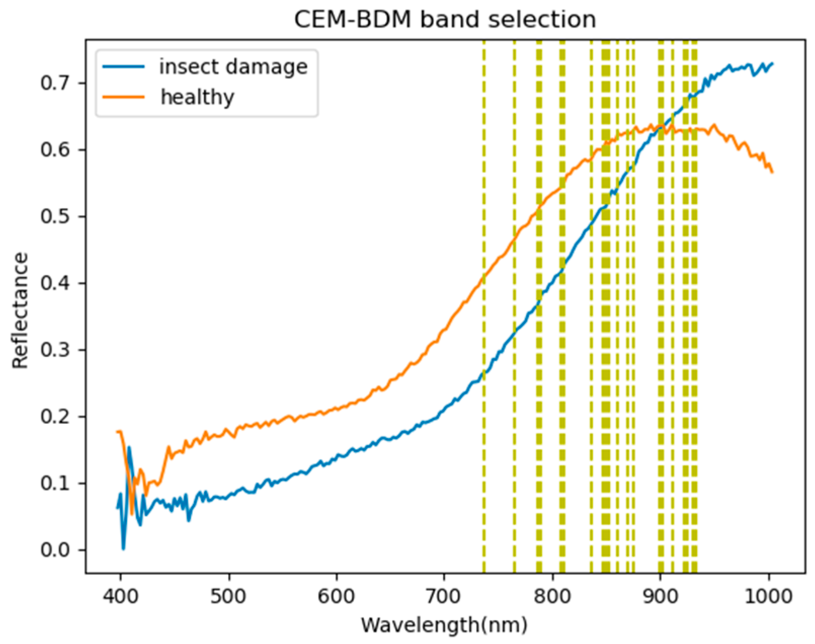
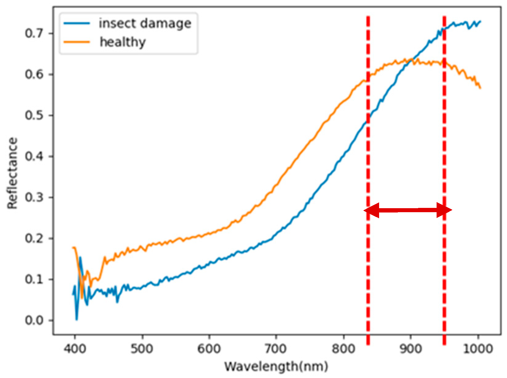
Based on the aforementioned results, this paper found that the number of bands is a critical factor. From the band selection results in Section 3.1, the foremost bands fell in the wavelength range of 850–950 nm. According to the spectral signature of healthy and insect damaged coffee beans in Figure 5, the most different spectrum was also between 850–950 nm. This finding can explain the above results, if the selected bands fell in this range, the results performed relatively well. Considering the number of bands, in the case of three bands, the CEM_BDM+CNN method had the best performance in ACC and Kappa, and the ACC was 95%, indicating that the minimization of inter-band correlation is helpful to detect insect damaged beans since the top three bands were between the range of 850–950 nm. In the 10 band and 20 band cases, the PCA+CNN method exhibited the best performance in ACC and kappa, which suggests that the covariance for band selection can determine the different bands between heathy and defective beans, and the effect was even improved when combined with CNN. Based on the above results, several findings can be observed as follows.

• As the background has many unknown signal sources responding to various wavelengths, the hyperspectral data collected in this paper were pre-processed to remove the background, which rendered the signal source in the image relatively simple. As too much spectral data increase the complexity of detection, only healthy coffee beans and insect damaged beans were included in the data for experimentation. Without other background noise interference, this experiment only required a few important bands to separate the insect damaged beans from healthy beans. The applied CEM-based band selection methods were based on the variance generated by CEM to rank the bands, where the top ranked bands are more representative and significant. Moreover, the basic assumption of PCA is that the data can find a vector projected in the feature space, and then the maximum variance of this group of data can be obtained, thus, it is also ranked by variance. In other words, the band selection methods with the variance as the standard can only use the top few bands to distinguish our experimental data with only two signal sources (healthy and unhealthy beans), which is supported by our experimental results. As the top few bandwidths are concentrated between 850 nm–950 nm, the difference between the spectral signature curves of the insect damaged beans and healthy beans could be easily observed between 850 nm–950 nm, as shown in Figure 51. The curve of healthy beans flattened, while the curve of the insect damaged beans rose beyond the range of 850 nm–950 nm, as shown in Figure 51.
• The greatest challenge in the detection of insect damaged coffee beans is that the damaged areas provide very limited spatial information and are generally difficult to visualize from data. CEM, which is a hyperspectral target detection algorithm, is effective in dealing with the subpixel detection problem [24,25,29,30]. As mentioned in Section 2.3.1, CEM requires only one desired spectral signature for detection, thus, the quality of the detection result is very sensitive to the desired spectral signature. To solve this problem, HIDDA applies OSGP to obtain a stable and improved spectral signature, thus the stability of detection can be increased. The second issue of CEM is that it only provides soft decision results; thus, this paper used linear SVM followed by CEM to obtain the hard decision results. The above-mentioned reasons are the key points that prove our proposed method, HIDDA, can perform well.
• The main problem of CNN during deep learning is that it requires a large number of training samples to learn more effectively and obtain suitable answers. Moreover, as our data consist of real images, there is no ground truth for us to label the insect damaged areas. To address this problem, HIDDA used CEM-OTSU to detect insect damaged beans, and used those pixels as the training samples for the CNN model. It is worth noting that we applied the results from CEM to generate more training samples for the CNN model, as CEM only requires one piece of knowledge of the target signature; hence, even though our training rate for CNN was low, the final results still performed well.
• In order for a comparison with prior studies,

  Table 7. The detailed comparison of prior studies.

  Ref.	Types	Training Rate	No. of Training	Testing Rate	No. of Testing	ACC (%)	Method	Image
  [2]	Normal	76%	200	24%	61	90.2	PCA+K-NN (k = 3) (5 PCA)	HSI
  	Black cherries	71%	5	29%	2	50
  	Black	68%	100	32%	45	80
  	Dehydrated	52%	100	48%	89	89.9
  [5]	Normal	unknown	444	unknown	161	97.52	K-NN (k = 10)	RGB
  	Black				169	97.04
  	Sour				165	92.12
  	Broken				166	94.45
  [6]	Normal	66%	70	34%	35	100	Thresholding	RGB
  	Black	66%	50	34%	25	100
  HIDDA	Normal	5%	30	95%	569	96.48	CEM-SVM (3 bands) CNN (3 bands)	HSI
  	Insect damage	5%	30	95%	570	93.33

  lists the detailed comparison of coffee beans. Several issues regarding our datasets, methods, and performance render this paper noticeable. First, HIDDA is the only method that detects insect damaged beans, which are more difficult to identify than black, sour, and broken beans. Second, HIDDA had the lowest training rate and highest testing rate with very good performance. Third, HIDDA is the only method, as proposed by CEM-SVM and the CNN model, that uses only three bands in the detection of insect damaged coffee beans. The authors [2] also used hyperspectral imaging (VIS-NIR) to identify black and broken beans, which extracted features through PCA and used K-NN for classification. However, in that paper, the number of beans was relatively too small, and final detection rate was lower than the proposed method of this paper. Other studies [5,6] have used traditional RGB images, which can only address targets according to the color and shape based on the spatial information, meaning that it can only identify black and broken beans. In contrast with prior studies, HIDDA is based on spectral information provided by hyperspectral sensors, which can detect targets at the subpixel level of insect damage, which has very limited spatial information.

4. Conclusions

Insect damage is the most commonly seen defect in coffee beans. The damaged areas are often smaller than the pixel resolution, thus, the targets to be detected are usually embedded in a single pixel. Therefore, the only way to detect and extract these targets is at the subpixel level, meaning traditional spatial domain (RGB)-based image processing techniques may not be suitable. To address this problem, this paper adopted spectral processing techniques that can characterize and capture the spectral information of targets, rather than their spatial information. After using a VIS-NIR push-broom hyperspectral imaging camera to obtain the images of green coffee beans, this paper further developed HIDDA, which includes six algorithms for band selection as well as CEM-SVM and CNN for identification. The experimental samples of this paper were 1139 coffee beans including 569 healthy beans and 570 defective beans. The accuracy in classifying healthy beans was 96.4%, and that in classifying defective beans was 93%; the overall accuracy was nearly 95%.

As CEM is one of the few algorithms that can suppress background noise while detecting the target at the subpixel level, the proposed method applies CEM as the kernel of the algorithm, which uses sampling correlation matrix R to suppress the background and a specific constraint in the FIR filter to pass through the target. CEM can easily implement binary classification as it only requires one knowledge of the target, and no other information is required, thus, CEM was used to design the band selection methods for CBS and CTBS, which use the CEM produced variance as criteria to select and rank the bands. This paper compared PCA as it also uses variance as the criteria. The results showed that the top few bands selected by the six band selection algorithms were concentrated between 850 nm–950 nm, which means that these bands are important and representative for identifying healthy beans and defective beans. Since no specific shape and color can be captured in the insect damaged beans, spectral information is needed to detect the insect damaged areas. In this case, this paper proposed the two spectral-based classifiers after obtaining the results of band selection. One combines CEM with the SVM for classification, while the other uses the neural network of 1D-CNN’s deep learning to implement binary classification. In order to consider future sensor design, this paper used three bands, 10 bands, and 20 bands for experimentation. The results showed that in the case of three bands, both CEM-SVM and CNN performed very well, indicating that HIDDA can detect insect damaged coffee beans within only a few bands.

In conclusion, this paper has several important contributions. First, hyperspectral images were used to detect insect damaged beans, which are more difficult to identify by visual inspection than other defective beans such as black and sour beans. Second, this paper applied the results from CEM to generate more training samples for the CNN and SVM models, and the training sample rate was relatively low. Moreover, as HIDDA only requires knowledge of one of the spectral data for insect damaged beans under only three bands, and the accuracy was nearly 95%. In other words, HIDDA is advantageous in the commercial development of sensors in the future. Third, six band selection methods were developed, analyzed, and combined with neural networks and deep learning. The accuracy in 20 images of 1100 coffee beans was 95%, and the kappa was 90%. The results indicate that the band in the wavelength of 850–950 nm is significant for identifying healthy beans and defective beans. Our future study will work toward commercialization in the coffee processing process, wherein, the experimental process will be combined with mechanical automation.

References

- Mutua, J.M. Post Harvest Handling and Processing of Coffee in African Countries; Food Agriculture Organization: Rome, Italy, 2000. [Google Scholar]
- Oliveri, P.; Malegori, C.; Casale, M.; Tartacca, E.; Salvatori, G. An innovative multivariate strategy for HSI-NIR images to automatically detect defects in green coffee. Talanta 2019, 199, 270–276. [Google Scholar] [CrossRef] [PubMed]
- Caporaso, N.; Whitworth, M.B.; Grebby, S.; Fisk, I. Rapid prediction of single green coffee bean moisture and lipid content by hyperspectral imaging. J. Food Eng. 2018, 227, 18–29. [Google Scholar] [CrossRef] [PubMed]
- Zhang, C.; Liu, F.; He, Y. Identification of coffee bean varieties using hyperspectral imaging: Influence of preprocessing methods and pixel-wise spectra analysis. Sci. Rep. 2018, 8, 2166. [Google Scholar] [CrossRef] [PubMed]
- García, M.; Candelo-Becerra, J.E.; Hoyos, F.E. Quality and Defect Inspection of Green Coffee Beans Using a Computer Vision System. Appl. Sci. 2019, 9, 4195. [Google Scholar] [CrossRef] [Green Version]
- Arboleda, E.R.; Fajardo, A.C.; Medina, R.P. An image processing technique for coffee black beans identification. In Proceedings of the 2018 IEEE International Conference on Innovative Research and Development (ICIRD), Bangkok, Thailand, 11–12 May 2018; pp. 1–5. [Google Scholar] [CrossRef]
- Clarke, R.J.; Macrae, R. Coffee; Springer Science and Business Media LLC: Berlin, Germany, 1987; p. 2. [Google Scholar]
- Mazzafera, P. Chemical composition of defective coffee beans. Food Chem. 1999, 64, 547–554. [Google Scholar] [CrossRef]
- Franca, A.S.; Oliveira, L.S. Chemistry of Defective Coffee Beans. In Food Chemistry Research Developments; Koeffer, E.N., Ed.; Nova Publishers: Newyork, NY, USA, January 2008; pp. 105–138. [Google Scholar]
- Chang, C.-I.; Du, Q.; Sun, T.-L.; Althouse, M. A joint band prioritization and band-decorrelation approach to band selection for hyperspectral image classification. IEEE Trans. Geosci. Remote. Sens. 1999, 37, 2631–2641. [Google Scholar] [CrossRef] [Green Version]
- Chang, C.-I.; Wang, S. Constrained band selection for hyperspectral imagery. IEEE Trans. Geosci. Remote Sens. Jun. 2006, 44, 1575–1585. [Google Scholar] [CrossRef]
- Liu, K.-H.; Chen, S.-Y.; Chien, H.-C.; Lu, M.-H. Progressive Sample Processing of Band Selection for Hyperspectral Image Transmission. Remote. Sens. 2018, 10, 367. [Google Scholar] [CrossRef] [Green Version]
- Su, H.; Du, Q.; Chen, G.; Du, P. Optimized Hyperspectral Band Selection Using Particle Swarm Optimization. IEEE J. Sel. Top. Appl. Earth Obs. Remote. Sens. 2014, 7, 2659–2670. [Google Scholar] [CrossRef]
- Su, H.; Gourley, J.J.; Du, Q. Hyperspectral Band Selection Using Improved Firefly Algorithm. IEEE Geosci. Remote. Sens. Lett. 2016, 13, 68–72. [Google Scholar] [CrossRef]
- Yuan, Y.; Zhu, G.; Wang, Q. Hyperspectral Band Selection by Multitask Sparsity Pursuit. IEEE Trans. Geosci. Remote. Sens. 2015, 53, 631–644. [Google Scholar] [CrossRef]
- Yuan, Y.; Zheng, X.; Lu, X. Discovering Diverse Subset for Unsupervised Hyperspectral Band Selection. IEEE Trans. Image Process. 2016, 26, 51–64. [Google Scholar] [CrossRef]
- Wang, C.; Gong, M.; Zhang, M.; Chan, Y. Unsupervised Hyperspectral Image Band Selection via Column Subset Selection. IEEE Geosci. Remote. Sens. Lett. 2015, 12, 1411–1415. [Google Scholar] [CrossRef]
- Dorrepaal, R.; Malegori, C.; Gowen, A. Tutorial: Time Series Hyperspectral Image Analysis. J. Near Infrared Spectrosc. 2016, 24, 89–107. [Google Scholar] [CrossRef] [Green Version]
- Chang, C.-I. Hyperspectral Data Processing; Wiley: Hoboken, NJ, USA, 2013. [Google Scholar]
- Harsanyi, J.C. Detection and Classification of Subpixel Spectral Signatures in Hyperspectral Image Sequences. Ph.D. Thesis, Department of Electrical Engineering, University of Maryland Baltimore County, College Park, MD, USA, August 1993. [Google Scholar]
- Farrand, W.H.; Harsanyi, J.C. Mapping the distribution of mine tailings in the Coeur d’Alene river valley, Idaho, through the use of a constrained energy minimization technique. Remote Sens. Environ. Jan. 1997, 59, 64–76. [Google Scholar] [CrossRef]
- Chang, C.-I. Target signature-constrained mixed pixel classification for hyperspectral imagery. IEEE Trans. Geosci. Remote. Sens. 2002, 40, 1065–1081. [Google Scholar] [CrossRef] [Green Version]
- Chang, C.-I. Hyperspectral Imaging: Techniques for Spectral Detection and Classification; Kluwer Academic/Plenum Publishers: Dordrecht, The Netherlands, 2003. [Google Scholar]
- Lin, C.; Chen, S.-Y.; Chen, C.-C.; Tai, C.-H. Detecting newly grown tree leaves from unmanned-aerial-vehicle images using hyperspectral target detection techniques. ISPRS J. Photogramm. Remote. Sens. 2018, 142, 174–189. [Google Scholar] [CrossRef]
- Wang, Y.; Wang, L.; Yu, C.; Zhao, E.; Song, M.; Wen, C.-H.; Chang, C.-I. Constrained-Target Band Selection for Multiple-Target Detection. IEEE Trans. Geosci. Remote. Sens. 2019, 57, 6079–6103. [Google Scholar] [CrossRef]
- Chang, C.-I. Real-Time Progressive Hyperspectral Image Processing: Endmember Finding and Anomaly Detection; Springer: New York, NY, USA, 2016. [Google Scholar]
- Pudil, P.; Novovicova, J.; Kittler, J. Floating search methods in feature selection. Pattern Recognit. Lett. 1994, 15, 1119–1125. [Google Scholar] [CrossRef]
- Pearson, K. LIII. On lines and planes of closest fit to systems of points in space. Philos. Mag. 1901, 2, 559–572. [Google Scholar] [CrossRef] [Green Version]
- Chen, S.-Y.; Lin, C.; Tai, C.-H.; Chuang, S.-J. Adaptive Window-Based Constrained Energy Minimization for Detection of Newly Grown Tree Leaves. Remote. Sens. 2018, 10, 96. [Google Scholar] [CrossRef] [Green Version]
- Chen, S.-Y.; Lin, C.; Chuang, S.-J.; Kao, Z.-Y. Weighted Background Suppression Target Detection Using Sparse Image Enhancement Technique for Newly Grown Tree Leaves. Remote. Sens. 2019, 11, 1081. [Google Scholar] [CrossRef] [Green Version]
- Otsu, N. A Threshold Selection Method from Gray-Level Histograms. IEEE Trans. Syst. Man Cybern. 1979, 9, 62–66. [Google Scholar] [CrossRef] [Green Version]
- Hinton, G.E.; Osindero, S.; Teh, Y.-W. A Fast Learning Algorithm for Deep Belief Nets. Neural Comput. 2006, 18, 1527–1554. [Google Scholar] [CrossRef] [PubMed]
- Bradshaw, D.; Gans, C.; Jones, P.; Rizzuto, G.; Steiner, N.; Mitton, W.; Ng, J.; Koester, R.; Hartzman, R.; Hurley, C. Novel HLA-A locus alleles including A*01012, A*0306, A*0308, A*2616, A*2617, A*3009, A*3206, A*3403, A*3602 and A*6604. Tissue Antigens 2002, 59, 325–327. [Google Scholar] [CrossRef] [PubMed]
- McCulloch, W.S.; Pitts, W. A logical calculus of the ideas immanent in nervous activity. Bull. Math. Boil. 1943, 5, 115–133. [Google Scholar] [CrossRef]
- Rumelhart, D.E.; Hinton, G.E.; Williams, R.J. Learning representations by back-propagating errors. Nature 1986, 323, 533–536. [Google Scholar] [CrossRef]
- Rosenblatt, F. The perceptron: A probabilistic model for information storage and organization in the brain. Psychol. Rev. 1958, 65, 386–408. [Google Scholar] [CrossRef] [Green Version]
- Zhao, B.; Lu, H.; Chen, S.; Liu, J.; Wu, D. Convolutional neural networks for time series classification. J. Syst. Eng. Electron. 2017, 28, 162–169. [Google Scholar] [CrossRef]
- Kiranyaz, S.; Avci, O.; Abdeljaber, O.; Ince, T.; Gabbouj, M.; Inman, D.J. 1D Convolutional Neural Networks and Applications: A Survey. arXiv 2019, arXiv:1905.03554. [Google Scholar]
- Cortes, C.; Vapnik, V. Support-Vector Networks. Mach. Learn. 1995, 20, 273–297. [Google Scholar] [CrossRef]
- Youden, W.J. Index for rating diagnostic tests. Cancer 1950, 3, 32–35. [Google Scholar] [CrossRef]
- Cohen, J. A Coefficient of Agreement for Nominal Scales. Educ. Psychol. Meas. 1960, 20, 37–46. [Google Scholar] [CrossRef]
- Cohen, J. Weighted kappa: Nominal scale agreement with provision for scaled disagreement or partial credit. Psychol. Bull. 1968, 70, 213–220. [Google Scholar] [CrossRef] [PubMed]
Figure 1.
Hyperspectral imaging system.
Figure 2.
Filming of coffee beans.
Figure 3.
Results of green coffee beans filming. (a) Color image; (b) 583 nm; (c) 636 nm; (d) 690 nm; (e) 745 nm; (f) 800 nm.
Figure 4.
The appearance of healthy and defective beans. (a) Healthy bean, (b) defective bean (black bean), (c) defective bean (insect damaged bean), and (d) a defective bean (broken bean).
Figure 5.
Spectral signature of the healthy and insect damaged coffee beans.
Figure 6.
The optimal signature generation process.
Figure 7.
The 1D-CNN model.
Figure 8.
The 1D-CNN model architecture.
Figure 9.
The hyperspectral insect damage detection algorithm flowchart. (a) Training data of Support Vector Machine (SVM), (b) Testing data of Support Vector Machine (SVM), (c) Training data of Convolutional Neural Networks (CNN) (d) Testing data of Convolutional Neural Networks (CNN).
Figure 10.
Visualization of the CEM_BDM band selection results. The first five bands are 933, 900, 869, 930, and 875 nm.
Figure 11.
Visualization of the MinV_BP band selection results. The first five bands are 936, 933, 927, 930, and 925 nm.
Figure 12.
Visualization of the MaxV_BP band selection results. The first five bands are 858, 927, 850, 674, and 891 nm.
Figure 13.
Visualization of the SF_CTBS band selection results. The first five bands are 936, 858, 534, 927, and 693 nm.
Figure 14.
Visualization of the SB_CTBS band selection results. The first five bands are 858, 850, 927, 674, and 891 nm.
Figure 15.
Visualization of the PCA band selection results. The first five bands are 936, 875, 872, 869, and 866 nm.
Figure 16.
Results of green coffee beans CEM-SVM+CEM_BDM three bands (a–d) SVM classification results, (e–h) final visual images.
Figure 17.
Results of green coffee beans CEM-SVM+ MinV_BP three bands (a–d) SVM classification results, (e–h) final visual images.
Figure 18.
Results of green coffee beans CEM-SVM+ MaxV _BP three bands (a–d) SVM classification results, (e–h) final visual images.
Figure 19.
Results of green coffee beans CEM-SVM+ SF_CTBS three bands (a–d) SVM classification results, (e–h) final visual images.
Figure 20.
Results of green coffee beans CEM-SVM+SB_CTBS three bands, (a–d) SVM classification results, (e–h) final visual images.
Figure 21.
Results of green coffee beans CEM-SVM+PCA, (a–d) SVM classification results, (e–h) final visual images.
Figure 22.
Results of green coffee beans CNN+CEM-BDM three bands, (a–d) CNN classification results, (e–h) final visual images.
Figure 23.
Results of green coffee beans CNN+ maxV_BP three bands, (a–d) CNN classification results, (e–h) final visual images.
Figure 24.
Results of green coffee beans CNN+SF_CTBS three bands, (a–d) CNN classification results, (e–h) final visual images.
Figure 25.
Results of green coffee beans CNN+SB_CTBS three bands, (a–d) CNN classification results, (e–h) final visual images.
Figure 26.
Results of green coffee beans CNN+ PCA three bands, (a–d) CNN classification results, (e–h) final visual images.
Figure 27.
Results of green coffee bean CEM-SVM+CEM_BDM 10 bands. (a–d) SVM classification results, (e–h) final visual images.
Figure 28.
Results of green coffee bean CEM-SVM+ MinV_BP 10 bands. (a–d) SVM classification results, (e–h) final visual images.
Figure 29.
Results of green coffee bean CEM-SVM+ MaxV_BP 10 bands. (a–d) SVM classification results, (e–h) final visual images.
Figure 30.
Results of green coffee bean CEM-SVM+ SF_CTBS 10 bands. (a–d) SVM classification results, (e–h) final visual images.
Figure 31.
Results of green coffee bean CEM-SVM+ SB_CTBS 10 bands. (a–d) SVM classification results, (e–h) final visual images.
Figure 32.
Results of green coffee bean CEM-SVM+PCA 10 bands. (a–d) SVM classification results, (e–h) final visual images.
Figure 33.
Results of green coffee bean CNN+CEM_BDM 10 bands. (a–d) CNN classification results, (e–h) final visual images.
Figure 34.
Results of green coffee bean CNN + maxV_BP 10 bands. (a–d) CNN classification results, (e–h) final visual images.
Figure 35.
Results of green coffee bean CNN+SF_CTBS 10 bands. (a–d) CNN classification results, (e–h) final visual images.
Figure 36.
Results of green coffee bean CNN+SB_CTBS 10 bands. (a–d) CNN classification results, (e–h) final visual images.
Figure 37.
Results of green coffee bean CNN+PCA 10 bands. (a–d) CNN classification results, (e–h) final visual images.
Figure 38.
Results of green coffee beans CEM-SVM+CEM_BDM 20 bands. (a–d) SVM classification results, (e–h) final visual images.
Figure 39.
Results of green coffee bean CEM-SVM+MinV_BP 20 bands. (a–d) SVM classification results, (e–h) final visual images.
Figure 40.
Results of green coffee bean CEM-SVM+MaxV_BP 20 bands. (a–d) SVM classification results, (e–h) final visual images.
Figure 41.
Results of green coffee bean CEM-SVM+SF_CTBS 20 bands. (a–d) SVM classification results, (e–h) final visual images.
Figure 42.
Results of green coffee bean CEM-SVM+SB_CTBS 20 bands. (a–d) SVM classification results, (e–h) final visual images.
Figure 43.
Results of green coffee bean CEM-SVM+PCA 20 bands. (a–d) SVM classification results, (e–h) final visual images.
Figure 44.
Results of green coffee bean CNN+CEM_BDM 20 bands. (a–d) CNN classification results, (e–h) final visual images.
Figure 45.
Results of green coffee bean CNN+maxV_BP 20 bands. (a–d) CNN classification results, (e–h) final visual images.
Figure 46.
Results of green coffee bean CNN+SF_CTBS 20 bands. (a–d) CNN classification results, (e–h) final visual images.
Figure 47.
Results of green coffee bean CNN+SB_CTBS 20 bands. (a–d) CNN classification results, (e–h) final visual images.
Figure 48.
Results of green coffee bean CNN+PCA 20 bands. (a–d) CNN classification results, (e–h) final visual images.
Figure 49.
The ACC accuracy histograms of 3 bands, 10 bands, and 20 bands.
Figure 50.
The Kappa histograms of 3 bands, 10 bands, and 20 bands.
Figure 51.
Highlight of the spectral signature for healthy and insect damaged beans.