Using Artificial Neural Networks and Remotely Sensed Data to Evaluate the Relative Importance of Variables for Prediction of Within-Field Corn and Soybean Yields

Abstract

Crop yield prediction prior to harvest is important for crop income and insurance projections, and for evaluating food security. Yet, modeling crop yield is challenging because of the complexity of the relationships between crop growth and predictor variables, especially at the field scale. In this study, an artificial neural network (ANN) method was used: (1) to evaluate the relative importance of predictor variables for the prediction of within-field corn and soybean end-of-season yield and (2) to evaluate the performance of the ANN models with a minimal optimized variable dataset for their capacity to predict corn and soybean yield over multiple years at the within-field level. Several satellite derived vegetation indices (normalized difference vegetation index—NDVI, red edge NDVI and simple ratio—SR) and elevation derived variables (slope, flow accumulation, aspect) were used as crop yield predictor variables, hypothesizing that the different variables reflect different crop and site conditions. The study identified the SR index and the slope as the most important predictor variables for both crop types during two training and testing years (2011, 2012). The dates of the most important SR images, however, were different for the two crop types and corresponded to their critical crop developmental stages (phenology). The relative mean absolute errors were overall smaller for corn compared to soybean: all of the 2011 corn study fields had errors below 10%; 75% of the fields had errors below 10% in 2012. The errors were more variable for soybean. In 2011, 37% of the fields had errors below 10%, while in 2012, 100% of the fields had errors below 20%. The results are promising and can provide yield estimates at the farm level, which could be useful in refining broader scale (e.g., county, region) yield projections.

1. Introduction

The ability to predict crop yield prior to harvest is important for crop income and insurance projections, as well as for evaluating food security at local to global scales. Furthermore, models that spatially predict within-field yields can be used to characterize the environmental and management factors that most strongly contribute to yield variability. Information on these factors can support decision making on precision farming applications, agriculture practices, optimal types for crops to grow (i.e., rotation) and the selection of agriculture lands to be retired for the purpose of biodiversity/conservation. Crop yield can be predicted using a variety of statistical models and crop growth simulators via the use of critical crop, weather, soil, water availability and crop management information [1]. However, predicting crop yield variability in a field from year to year is challenging due the complexity of the relationships between crop growth and the driving factors, and the difficulty to characterize crop growth processes and the driving factors (e.g., varieties, soil management, fertilizer types).

Machine learning algorithms (MLAs), such as artificial neural networks (ANNs), are particularly useful for studying complex biological systems, as they can efficiently capture non-linear relationships and complex interactions among the driving variables [2]. MLAs have shown considerable promise in agricultural remote sensing applications, such as the retrieval of terrestrial vegetation biophysical properties [3,4]. Weiss et al. [3] emphasized three main growth areas associated with machine learning in agriculture: (1) the development of MLAs for classification, (2) the development of MLAs that can accelerate 3D physical models, and (3) the development of MLAs to retrieve crop variables.

Several studies have documented successful applications of MLAs to predict crop type [5], crop phenology [6] and crop yield [7,8,9,10,11,12,13,14,15,16,17]. Li et al. [13] used the normalized difference vegetation index NDVI derived from the moderate resolution imaging spectroradiometer MODIS) and the advanced very high resolution radiometer (AVHRR images in combination with a feed-forward multi-layer perceptron (MLP) ANN to predict corn and soybean yields at large spatial scales (county level). Using AVHRR-derived data in combination with an ANN model, Jiang et al. [17] reported good performance of the model for the prediction of count-scale winter wheat yield in China. In addition to the NDVI, this study also included other remotely sensed information, such as absorbed photosynthetically active radiation (APAR), canopy surface temperature, and a water stress index to reflect factors that affect winter wheat yield including: insolation, temperature water stress and soil conditions. Kaul et al. [14] used an ANN model for the prediction of corn and soybean yields at local to regional scales using historical yield data, a soil-rating index and weekly and monthly rainfall. They reported the importance of including weekly rainfall data and a soil index for increased prediction accuracy. At the field level, Fiezal et al. [12] used a combination of optical (Spot 4, 5 and Formosat-2) and microwave images (TerraSAR-X and RADARSAT-2) in combination with an ANN model to predict corn yield in France. They reported the capacity to predict yield up to three months before the harvest using the red reflectance and C-band (wavelength ~5.6 cm) backscatter at horizontal transmit/horizontal receive (HH) polarization. A few studies have also focused on the identification of important crop yield predictor variables and reported the importance of topographic attributes, crop hybrid, soil cation exchange capacity and soil micronutrients [18,19].

While an increasing number of studies have reported success using ANNs for crop yield prediction, most of these studies focused on predictions over larger regional scales. Large-scale studies are not always suitable for capturing critical site-specific factors that drive inter-region or in-field variability in crop productivity, which is a necessity for improving regional predictions of crop yield that are germane for many crop risk assessments and precision agriculture applications. The use of ANN predictive analytics for field-scale crop productivity assessments is not well documented compared to larger scale applications. As such, the objectives of this study were: (1) to evaluate the relative importance of predictor variables for the prediction of within-field corn and soybean end-of-season yield and (2) to evaluate the performance of the ANN models with a minimal optimized variable dataset for their capacity to predict corn and soybean yield over multiple years at the within- field level using high-resolution remotely sensed data.

2. Materials and Methods

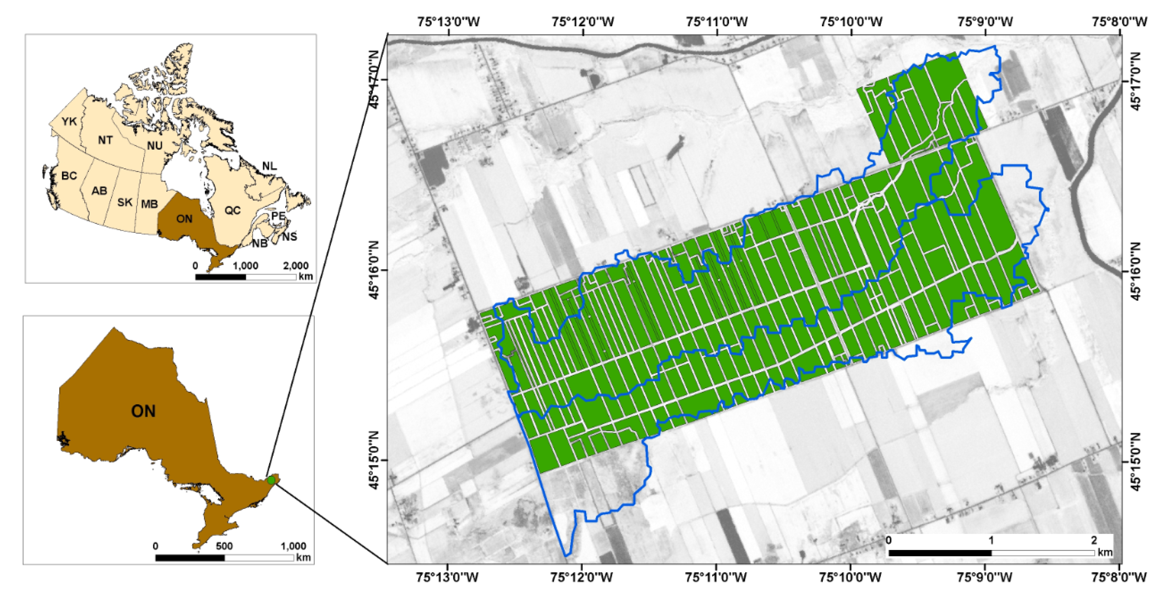
2.1. Study Area

The study was conducted on a tile-drained experimental watershed in eastern Ontario, Canada (45.26 N, 75.18 W; Figure 1). Corn (Zea mays L.) and soybean (Glycine max L.) are the two dominant crops in this region of Canada and in 2016, Ontario accounted for ~60% of national grain corn acreage and ~50% of national soybean acreage [20,21]. Corn and soybean are the two primary livestock and cash crops grown in the experimental watersheds. These crops are typically planted in May and harvested in September to October. In the study area, both crops were planted at the same time every year. Crop row spacing was around 50 cm for soybean and 60 cm for corn. Soybean and corn plant densities were generally 354,000 and 64,200 plants/ha, respectively. Fall moldboard plowing and spring cultivation using chisel-style implements were the main tillage practices employed on the site. Fertilizer generally consisted of the broadcast application of granular urea prior to planting and a granular starter application. Fertilizer rates were generally ~170 kg N/ha for corn and ~3 kg N/ha for soybean, depending on soil and crop requirements. More details about the study area and agriculture practices—including tiling systems—are described by Sunohara et al. [22].

2.2. Data

2.2.1. Field Data

Corn and soybean yield data were obtained from cooperating farmers for the years 2011, 2012 and 2016, matching the available satellite images. The data were collected during harvest using a John Deere combine harvester equipped with a GREENSTAR™ Yield Monitor System (John Deere, Moline, Illinois). Post-processing was done using Field Operations Viewer (version 2003.11.01; MapShots, San Francisco, California) and Yield Editor (Version 2.0.7; USDA-ARS Cropping Systems and Water Quality Research, Columbia, Missouri) and resulted in a dense point dataset with yields expressed in kg/ha. Points with yield values equal to the mean ± three times the standard deviation were considered outliers and eliminated. The summary statistics of corn and soybean yields for 2011, 2012 and 2016 are given in

Table 1. Summary statistics of corn and soybean yields for years of study.

Year	Crop	Average (kg/ha)	Standard Deviation (kg/ha)	Coefficient of Variation (%) 1	Total Precipitation May–August (mm) (360 mm) 2
2011	Corn	13619	1013	8	319.80
	Soybean	4200	1191	29
2012	Corn	11819	1245	11	205.40
	Soybean	3996	497	12
2016	Corn	12547	1380	11	284.80
	Soybean	3890	364	10

¹ The coefficient of variation (CV) of the observed yield was calculated as ((Standard deviation/average) * 100). ² 1981–2010 normal: Environment Canada, Russel Station, ON. http://weather.gc.ca (accessed on 3 April 2020).

and Figure 2a,b. The field yield data was used to train and test the ANN models.

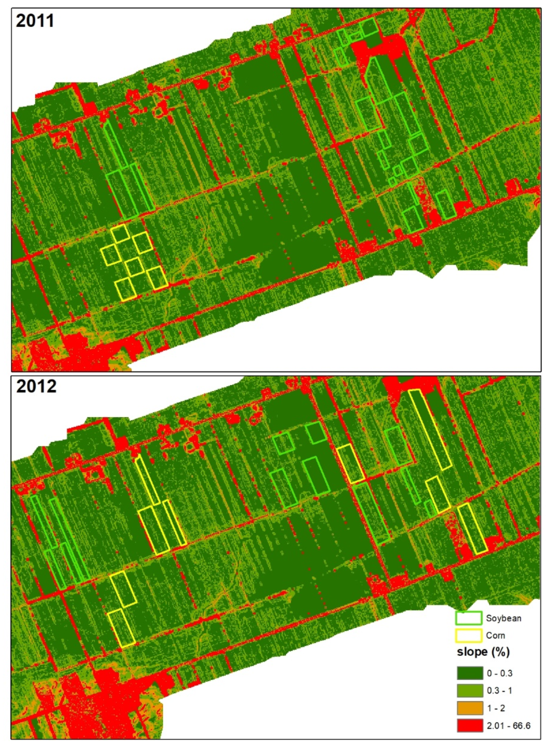
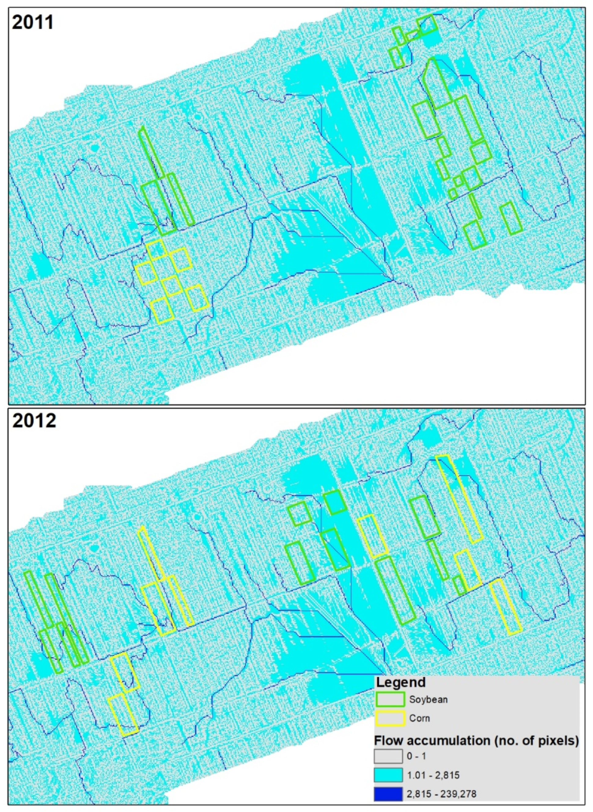
2.2.2. LIDAR and Topographic Derivatives

Based on the reported importance of micro-topographic attributes on crop growth properties [18,19,23], we included Lidar-derived variables to represent the micro-topography of the fields over this low topographic relief study area. Lidar data were collected over the experimental site by GeoDigital (Sandy Springs, GA) in November 2011, and a 1-m spatial resolution digital terrain elevation dataset was derived from the Lidar point cloud using LAStools (rapidlasso GmbH, Gilching, Germany).

Slope (Figure 3), aspect (not shown) and flow accumulation (Figure 4) were derived from the elevation dataset using the spatial analyst ArcGIS toolset within Advangeo^®Prediction (v 2.0 for ArcGIS 10.1; Beak Consultants GmbH, Freiberg, Germany).

The flow accumulation variable was calculated as the number of cells that flowed into each downslope cell (Figure 4). Higher relative flow accumulation numbers indicate areas of concentrated flow and can be used to determine stream channels, swales or depressions. Cells with a value of 0 indicate local topographic highs with no upstream catchment area, such as knolls and ridges (see https://pro.arcgis.com/en/pro-app/tool-reference/spatial-analyst).

2.2.3. Optical Remote Sensing Derived Data

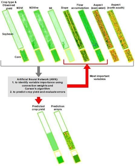
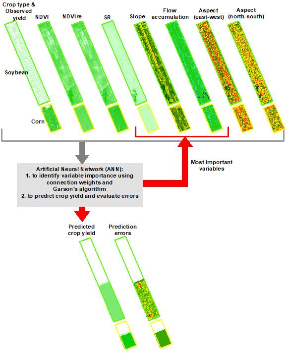
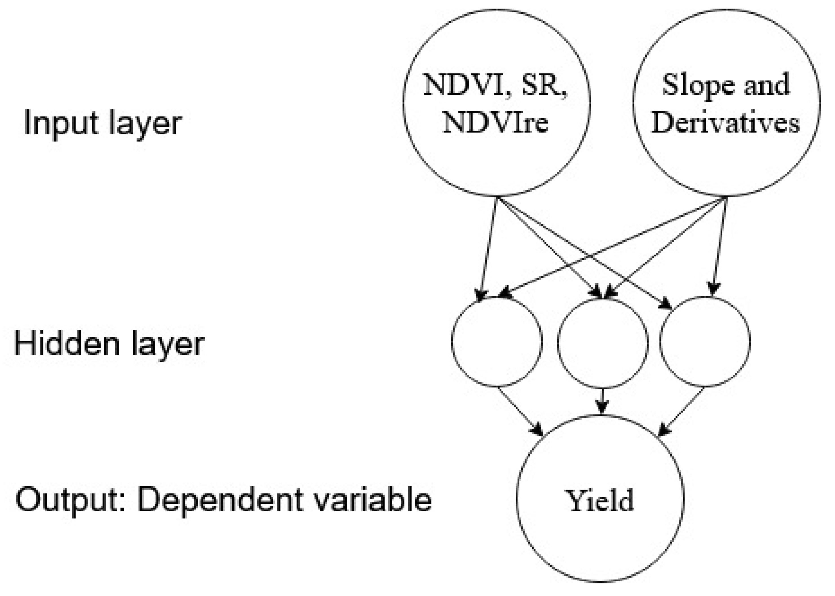
A total of 18 RapidEye images (5 m spatial resolution) were collected over the three study years (

Table 2. Summary of satellite images and their characteristics.

Satellite Sensors	Dates	Bands (nm)
RapidEye	2011: June 10, June 27, July 05, July 22, July 23, August 12, August 19 2012: June 17, June 21, June 28, July 11, July 18, July 29, August 04, August 18 2016: June 25, July 20, August 26	Blue (440–510), Green (520–590), Red (630–685), Red Edge (690–730), NIR (760–850)

). The RapidEye constellation consists of five satellites that are equipped with identical sensors and located within the same orbital plane. This setting allows the constellation to acquire high-resolution, large area image data on a daily basis (PlanetLabs Inc., https://www.planet.com/).

All images were georeferenced to the universal transverse Mercator coordinate system UTM 18N (with the world geodetic system—WGS-84 ellipsoid) and atmospherically corrected using ATCOR2 (PCI Geomatica v10.3, PCI Geomatics enterprises Inc, Ontario, Canada).

Considering the plethora of static and transient factors that can affect end-of-season yield in a field, we chose a set of satellite-derived vegetation and site spectral indices (

Table 3. Summary of spectral indices and their respective equations and references.

Spectral Indices	Equation	Reference
Normalized difference vegetation index (NDVI)	(RNIR − RRED)/(RNIR + RRED)	Rouse et al. (1974) 1
Simple ratio (SR)	RNIR/RRED	Jordan (1969) 2
Red edge normalized difference vegetation index (NDVIre)	(RNIR − RREDedge)/(RNIR + RREDedge)	Gitelson and Merzlyak (1994) 3

¹ Rouse, J.W., Haas, R.H., Schell, J.A., 1974. Monitoring the Vernal Advancement and Retrogradation (Greenwave Effect) of Natural Vegetation. Texas A and M University, College Station. ² Jordan, C.F., 1969. Derivation of leaf area index from quality of light on the forest floor. Ecology 50, 663–666. ³ Gitelson, A., Merzlyak, M.N., 1994. Spectral reflectance changes associated with autumn senescence of Aesculus hippocastanum L. and Acer platanoides L. Leaves. Spectral features and relation to chlorophyll estimation. J. Plant Physiol. 143, 286–292.

) to reflect plant nitrogen content, crop health (normalized difference vegetation index—NDVI and red edge NDVI—NDVIre) and crop canopy structure (Simple Ratio—R).

2.3. ANN Model

A review study on MLAs listed ANNs as one of the most successful MLAs for yield prediction, together with other methods like support vector regression, M5 prime regression trees, k-nearest neighbor and deep learning [24]. Our study used a parsimony approach to explore the importance of predictor variables and the performance of ANN models with a minimal variable set, in predicting crop yield within fields.

All predictor variables were clipped to the study area and the final spatial resolution of the model was set to the spatial resolution of the spectral indices from RapidEye (5 m). The 5-m resolution was considered via long-term field observations [22], to adequately capture most important micro-topographic features at the study site. A summary of all predictor variables used in the ANN analysis for each year is given in

Table 4. Predictor variables used in the ANN analysis for years 2011 and 2012.

Predictor Variables	2011	2012
Topographic attributes	Aspect south–north (degrees) Aspect west–east (degrees) Flow accumulation (number of pixels) Slope (%)	Aspect south–north (degrees) Aspect west–east (degrees) Flow accumulation (number of pixels) Slope (%)
Crop/canopy health	NDVI, NDVIre (June 10, June 27, July 05, July 22, July 23, August 12, August 19) (dimensionless)	NDVI, NDVIre (June 17, June 21, June 28, July 11, July 18, July 29, August 04, August 18) (dimensionless)
Crop/canopy structure	SR (June 10, June 27, July 05, July 22, July 23, August 12, August 19) (dimensionless)	SR (June 17, June 21, June 28, July 11, July 18, July 29, August 04, August 18) (dimensionless)
Landuse	Corn and soybean classes (categories)	Corn and soybean classes (categories)

.

We used the Advangeo^®Prediction Software, which uses a multilayer perceptron (MLP) ANN method to predict either classes or numeric values. Advangeo^®Prediction comes preloaded with defaults that have proven effective for many different applications [25]. In this study, we parsimoniously applied default parameters. An overview of the model is given in Figure 5.

The input layer receives the controlling parameters and the neurons of the hidden layer(s) and the output layer processes the weighted signals from the neurons of its previous layer and calculates an output value applying an activation function. The default parameters were: network topology (fully connected input layer and one hidden layer with three hidden neurons), activation function (for hidden and output layers: sigmoid with a steepness of 0.5), learning algorithm (derivative of back propagation algorithm), weight initialization (“initialize” algorithm of Widrow and Nguyen) and predefined stop parameters (number of epochs = 100 and mean square error − MSE border = 0.001). The input data consisted of different spatial layers of vegetation indices (SR, NDVI, NDVIre), Lidar derivatives (slope, aspect, flow accumulation), and crop type (corn, soybean). All the data were normalized to a scale of 0 to 1 (linear scaling) for use in the ANN model. The results were scaled back to the original data scales for error analysis.

The ANN model was trained and tested using 2011 data (fields were divided into 50% training vs. 50% testing), after which it was applied to 2012 and 2016 data. The same was done for 2012, where the model was trained and tested using 2012 data, and applied to 2011 and 2016 data. For each training year (2011, 2012), three main model scenarios were explored: (1) the network was trained with yield data from corn and soybean combined for the prediction of the within-field yield of the two crops, (2) the network was trained with soybean yield data only for the prediction of within-field soybean yield and (3) the network was trained with corn yield data only for the prediction of within-field corn yield (

Table 5. Overview of the model scenarios and number of pixels and fields used in error analysis ¹.

			Prediction Application Years and Crops
Training Year	Training Crop Yield	Model Names	Soybean 2011	Corn 2011	Soybean 2012	Corn 2012	Soybean 2016	Corn 2016
2011	Combined	PM001	19/23887 2	6/7082	22/23308	10/19109	9/12996	6/9960
	Soybean	PM004	19/23887		22/23308		9/12996
	Corn	PM006		6/7082		7/11894		6/9960
2012	Combined	PM015	19/23887	6/7082	12/11155	9/11296	9/12996	6/9960
	Soybean	PM019	19/23887		12/11155		9/12996
	Corn	PM021		6/7082		8/10241

¹ In some models, there was a difference in field numbers because of different input variables, cloud cover or the use of a subset of fields (test fields) versus all fields in some years. ² 19 = number of fields/23887 = number of pixels.

).

2.4. Analysis

The relative importance of the predictor variables for each modeling scenario was determined through connection weights and Garson’s algorithm [26]. Both methods are available in the Advangeo^®Prediction Software. For the model performance analysis, we used ANN models based on the predictor variables with the highest connection weights.

The performance of the models was evaluated by calculating the relative mean absolute error (RMAE) for fields using the following equations:

$$MA{E}_{field}=\frac{{\sum }_i^n\left|Predicted Yiel{d}_{pixel}-Observed Yiel{d}_{pixel}\right|}{n}$$

(1)

where MAE_field is the Mean Absolute Error of the field in kg/ha. Predicted Yield is the result from the ANN model and Observed Yield is yield data obtained from farmers. n is the number of pixels within a field.

$$RMA{E}_{Field}=\left(\frac{MA{E}_{Field}}{Mean Yiel{d}_{Field}}\right)· 100$$

(2)

where RMAE_field is in % and Mean Yield_Field is the average observed yield of the field, in kg/ha.

The RMAE was calculated for each field based on its number of pixels (Table 5). For each model, the RMAEs were then summarized to present the number of fields within each RMAE range.

The RMAEs were compared with the coefficient of variation (CV) of the observed yield to assess the magnitude of the errors. The CV was calculated as ((Standard deviation/average) ∗ 100

Spearman’s rank rho correlation coefficient was also reported to describe the relationship between predicted and observed crop yield. The correlation analysis was done for each model based on the number of fields.

3. Results and Discussion

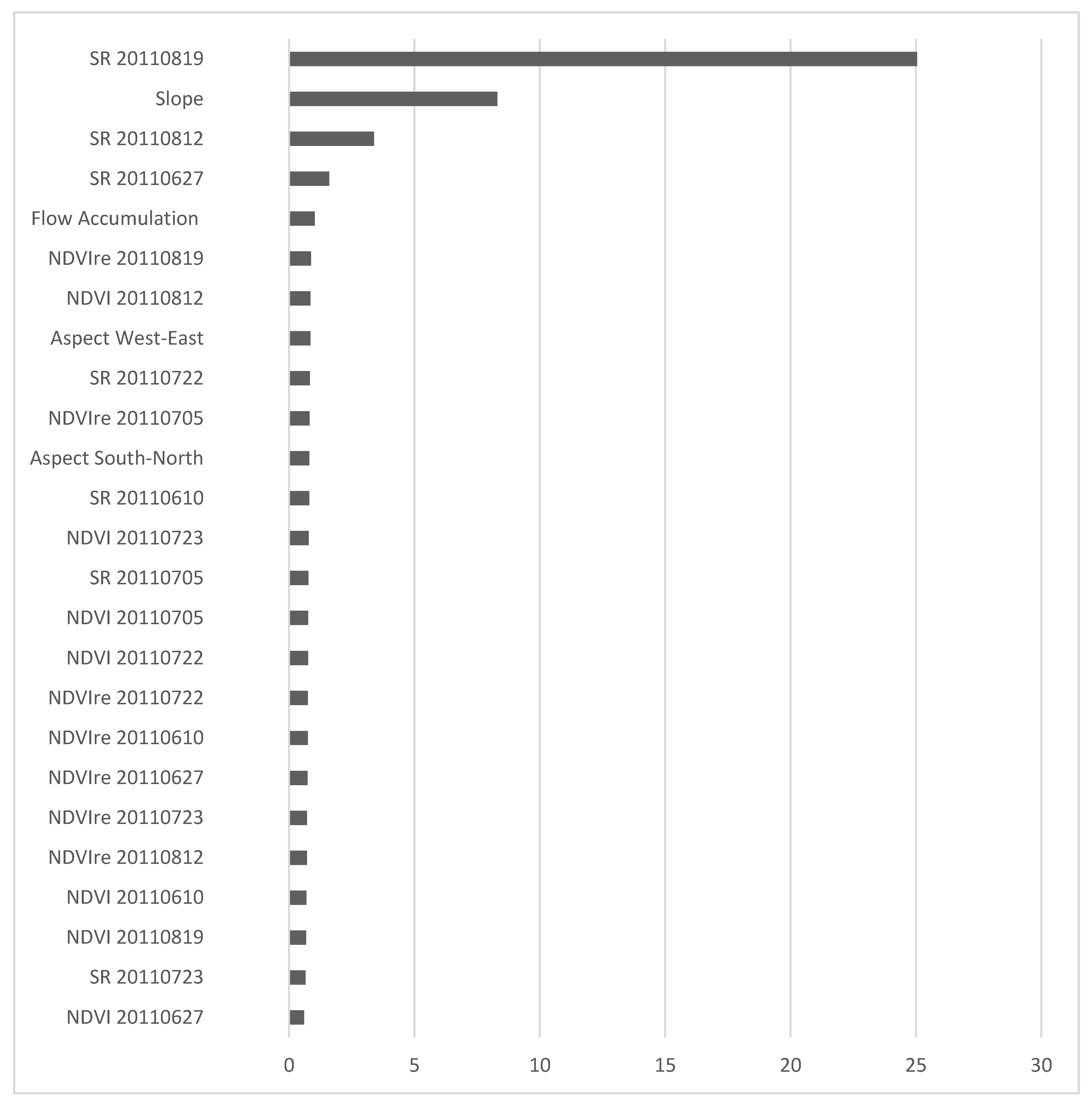
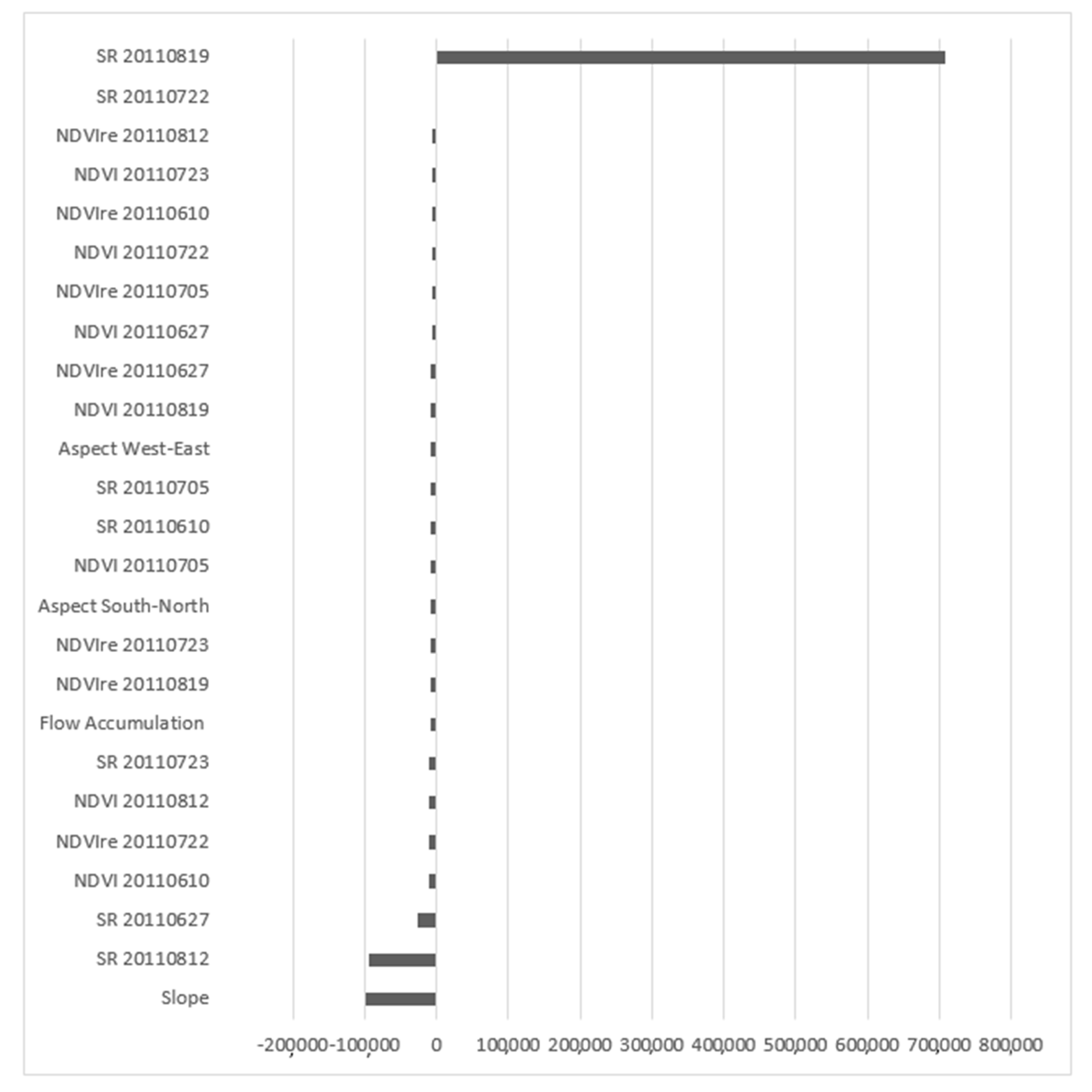
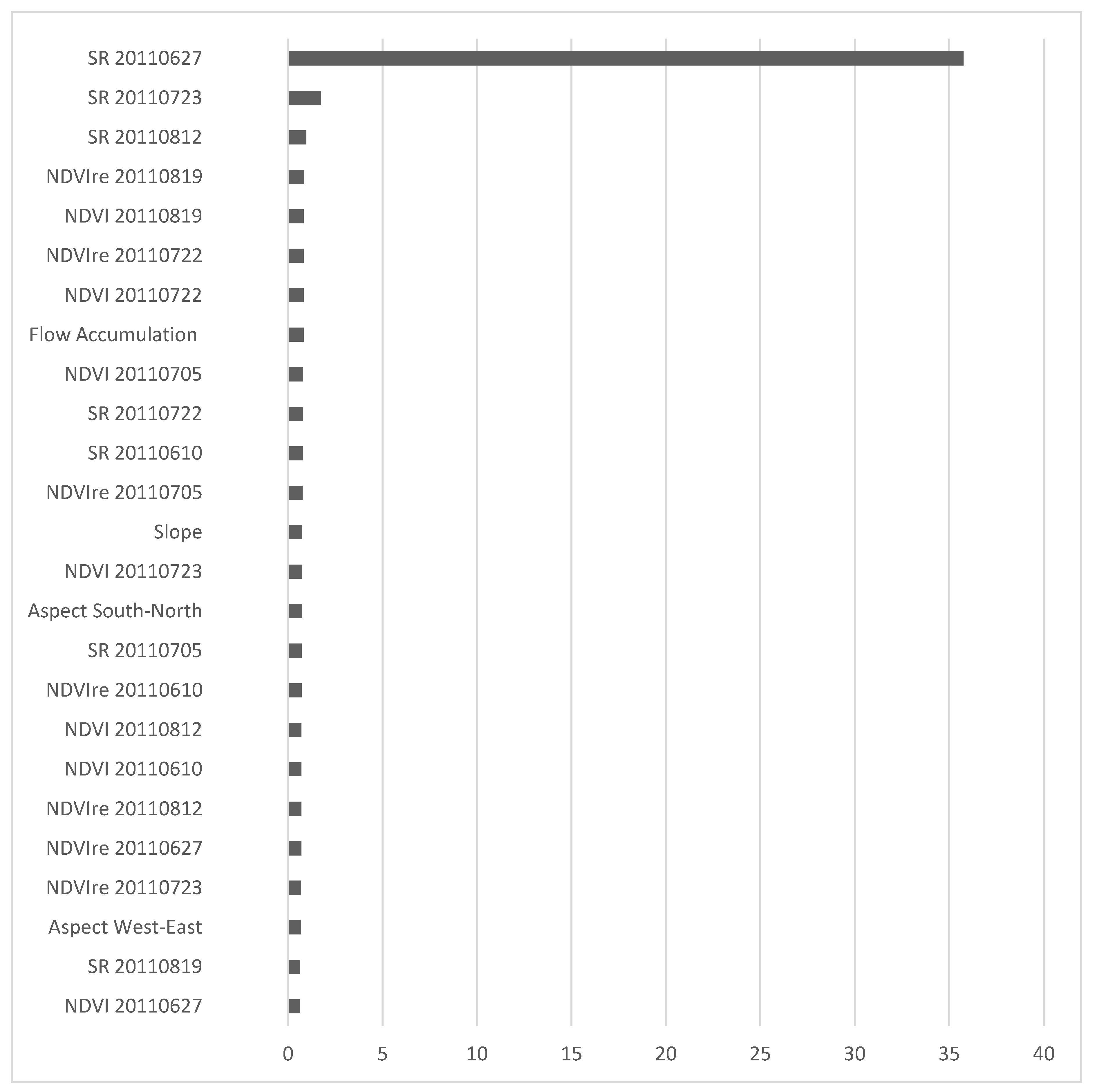
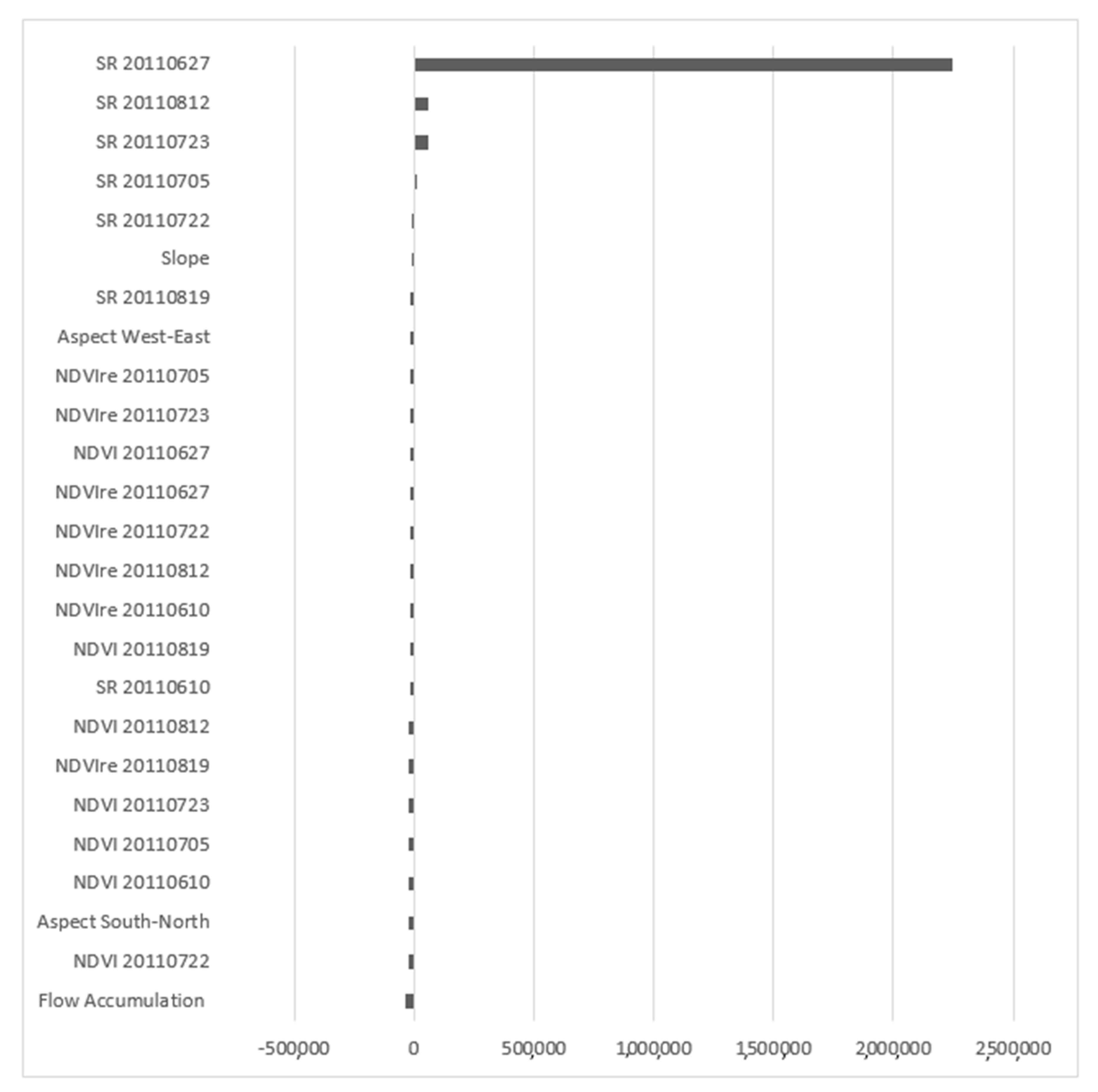
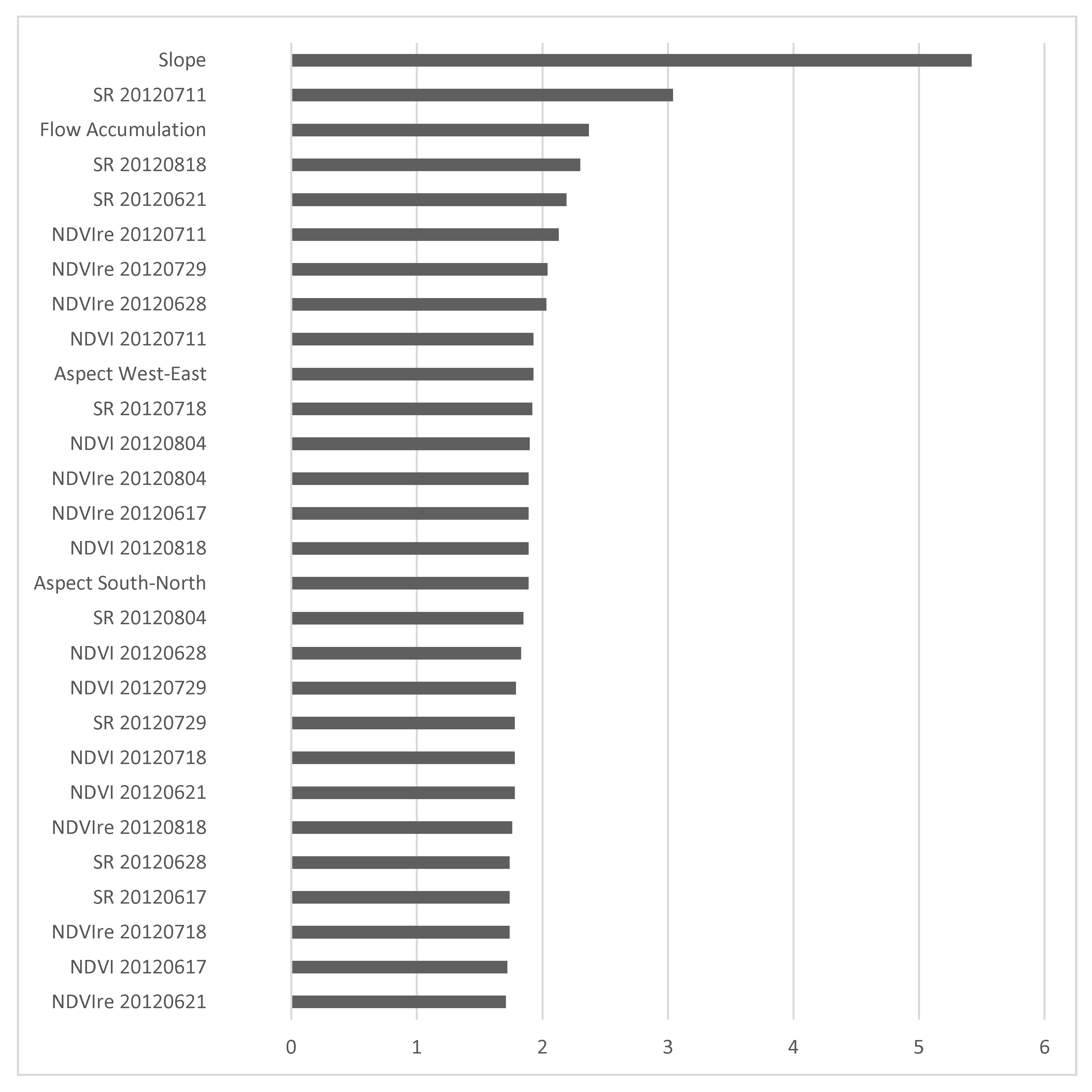
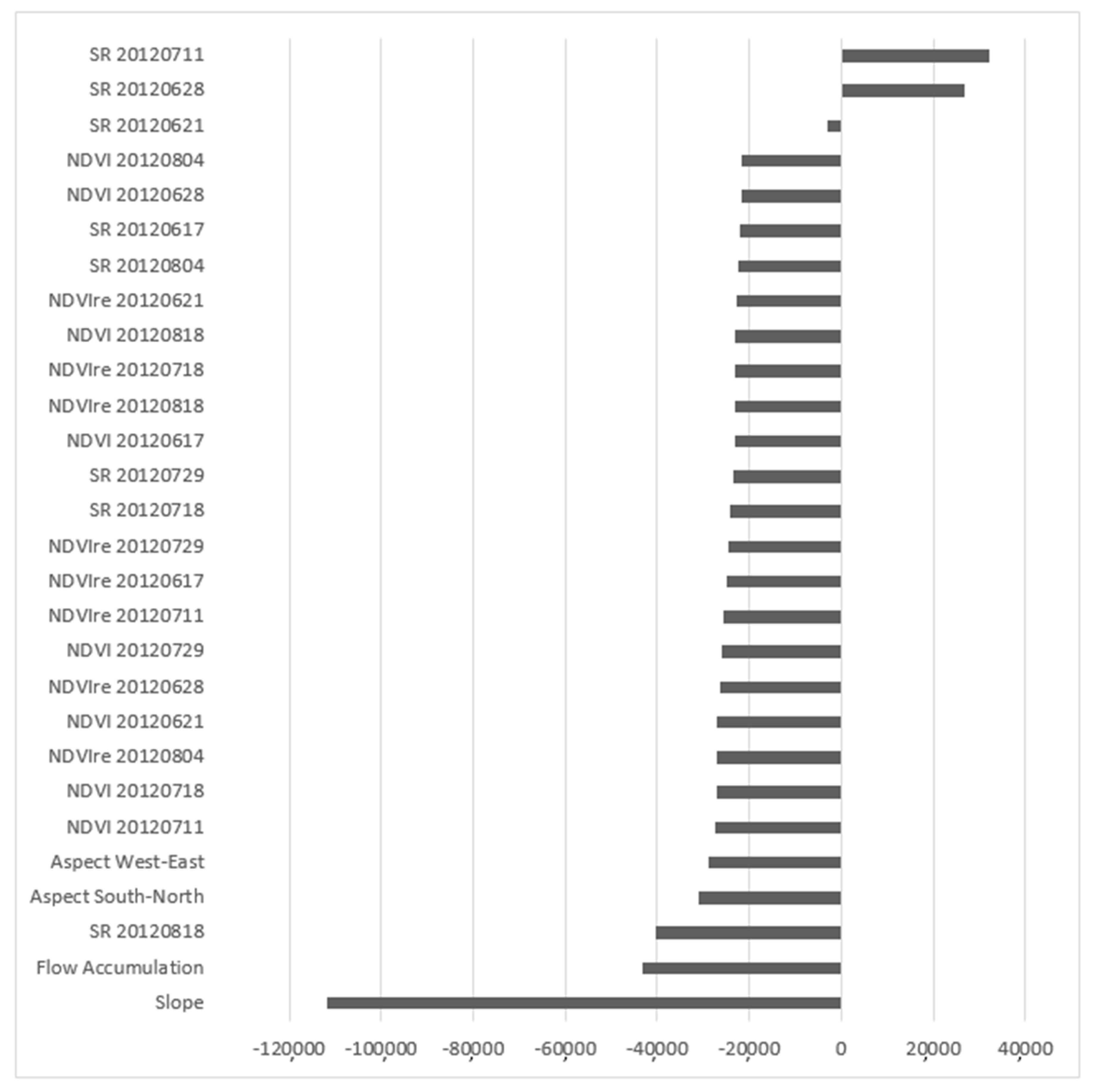
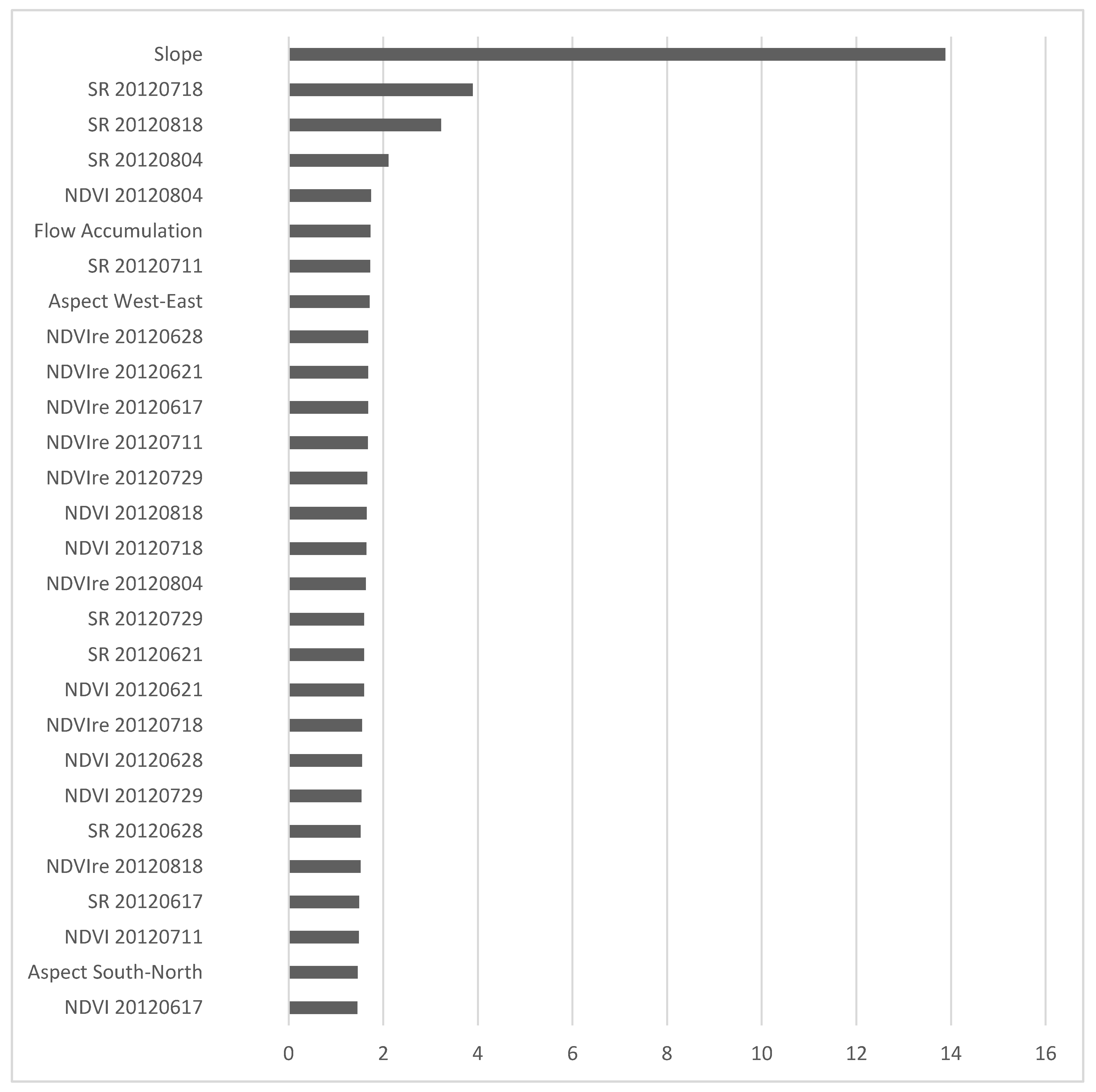
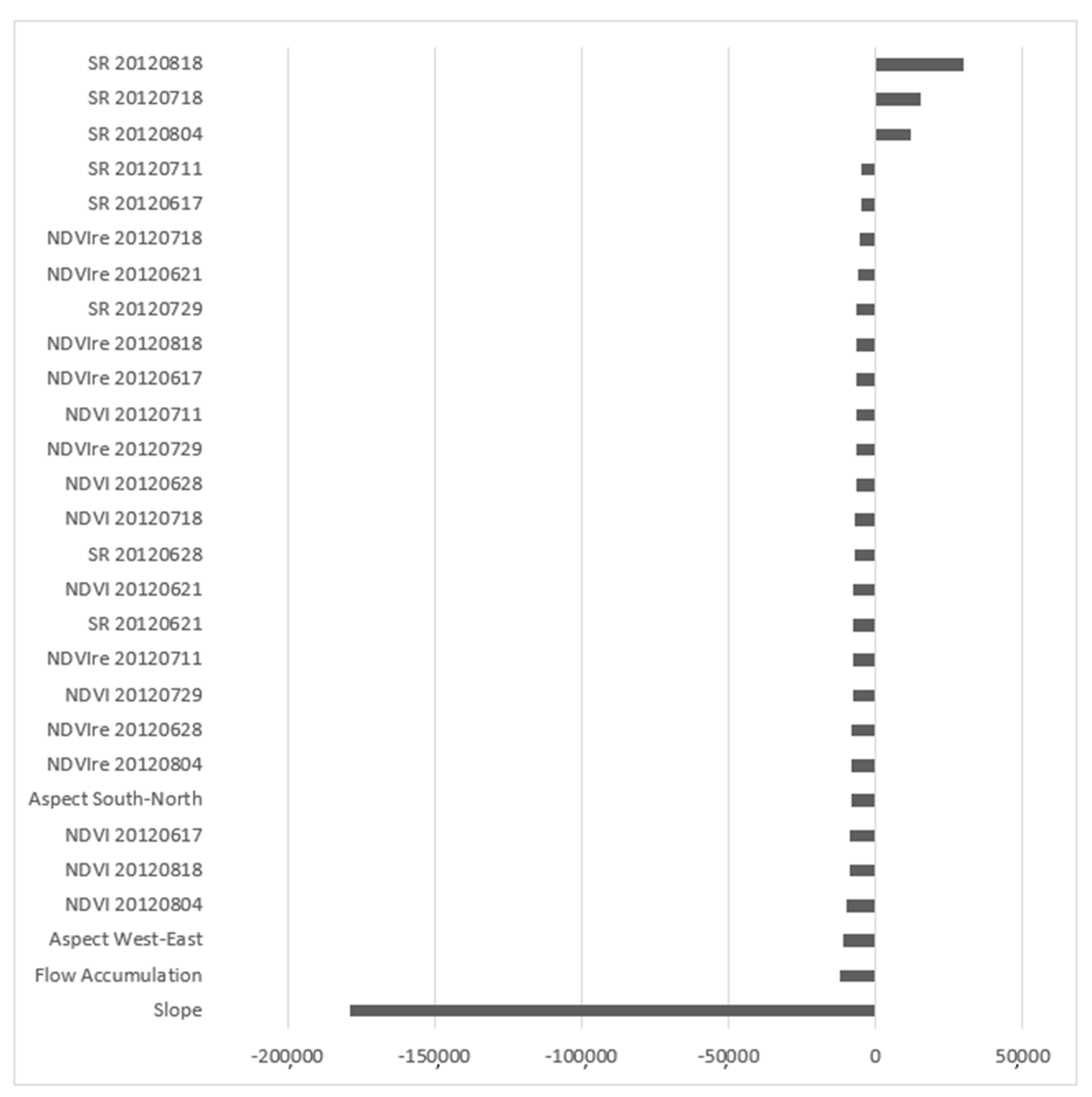
3.1. Relative Importance of Predictor Variables

Over 20 predictor variables (

Table 6. Overview of the input predictor variables and the most important predictor variables according to Garson’s algorithm and connection weights. Negative and positive signs for the most important predictor variables indicate the direction of their relationship with yield.

Yield Training Data	Input Predictor Variables	Most Important Predictor Variables Used in Final Optimized Models
Corn and Soybean (2011)	Slope, aspect, flow accumulation (2011), NDVIre, SR and NDVI (June 10, 27; July 05, 22, 23; Aug 12, 19)	SR August 19 (−), SR August 12 (−), Slope (−), SR June 27 (+)
Soybean (2011)		SR August 19 (+), Slope (−), SR August 12 (−), SR June 27 (−)
Corn (2011)		SR June 27 (+), SR July 23 (+)
Corn and Soybean (2012)	Slope, aspect, flow accumulation (2011), NDVIre, SR and NDVI (June 17, 21, 28; July 11, 18, 29; August 04, 18)	SR 29 July (−), SR 18 August (−), Slope (−), SR 28 June (+)
Soybean (2012)		Slope (−), SR 11 July (+), Flow accumulation (−), SR 18 August (−)
Corn (2012)		Slope (−), SR 18 July (+), SR 18 August (+), SR 04 August (−)

) were evaluated for their relevant importance for field-scale crop yield prediction. The results showed two variables with consistently high connection weights and Garson values for both crops: the SR indices and the slope (Table 6, Appendix A:

Table A1. Overview of the optimized prediction models and the predictor variables used in testing and application years.

				Prediction Application Years and Crops
				2011		2012		2016
Training Year	Training Crop Yield	Models	Optimized Models 2011	Soybean	Corn	Soybean	Corn	Soybean	Corn
2011	Combined	PM001	Slope (−) SR June 27 (+) SR August 12 (−) SR August 19 (−)	Slope SR June 27 SR August 12 SR August 19		Slope SR June 28 SR August 04 SR August 18		Slope SR June 25 SR July 20 SR August 26
	Soybean	PM004	Slope (−) SR June 27 (−) SR August 12 (−) SR August 19 (+)	Slope SR June 27 SR August 12 SR August 19		Slope SR June 28 SR August 04 SR August 18		Slope SR June 25 SR July 20 SR August 26
	Corn	PM006	SR June 27 (+) SR July 23 (+)		SR June 27 SR July 23		SR June 28 SR July 18		SR June 25 SR July 20
			Optimized models 2012	Soybean	Corn	Soybean	Corn	Soybean	Corn
2012	Combined	PM015	Slope (−) SR June 28 (+) SR July 29 (−) SR August 18 (−)	Slope SR June 27 SR July 23 SR August 19		Slope SR June 28 SR July 29 SR August 18		Slope SR June 25 SR July 20 SR August 26
	Soybean	PM019	Slope (−) Flow acc (−) SR July 11 (+) SR August 18 (−)	Slope Flow acc SR July 05 SR August 19		Slope Flow acc SR July 11 SR August 18		Slope Flow acc SR July 20 SR August 26
	Corn	PM021	Slope (−) SR July 18 (+) SR August 04 (−) SR August 18 (−)		Slope SR July 22 SR August 12 SR August 19		Slope SR July 18 SR August 04 SR August 18

).

The dates of the images, however, varied between crop types and between years. In the wetter year (2011), for example, the corn ANN model was optimized with only two relatively early SR images: one from June 27 (~V6, plant has six leaf collars, vegetative development stage) and one from July 23 (~VT–R1,

Table 7. Important development stages for corn and soybean.

Corn	Description
V12	Vegetative development stage: plant has 12 leaf collars
VT	Vegetative development stage: tassel emergence
R1	First reproductive development stage: silking
Soybean
R1	First reproductive development stage: beginning bloom
R4-R6	Reproductive stages R4 to R6, ranging from full pod (R4) to full seed (R6)

Summarized from Bagg et al. [27].

). The soybean model used two late-season images from August (R5-R6, Table 7), one image from June 27 (~V3, plant has three leaf collars, vegetative development stage) and the slope data. In the drier year (2012: cumulative May–August rainfall of ~205 mm), the images were similar for the two crops with the highest weights for July images (July 11: R1 for soybean; July 18: V11 for corn). Late season images were also used in the model: August 18 for both crops (R5–R6 for soybean, R4–R5 for corn) and August 04 for corn (~R3). The slope and flow accumulation were important for soybean (Table 6, Appendix A: Table A1).

The difference in image dates between the two crops is related to critical development stages of each crop type (Table 7). Corn is susceptible to water and nutrient deficiencies around the V12 and R1 stages [27], stages that closely match the image dates from both 2011 (July 23) and 2012 (July). Soybean is more susceptible to water and nutrient deficiencies around the reproductive stages R1, R4 and R6 [27]. These stages also match the image dates closely in 2011 (August 12 and 19) and 2012 (August 18).

Both Garson’s algorithm and the connection weights showed the highest weights for images acquired close to the critical crop development stages given in Table 7.

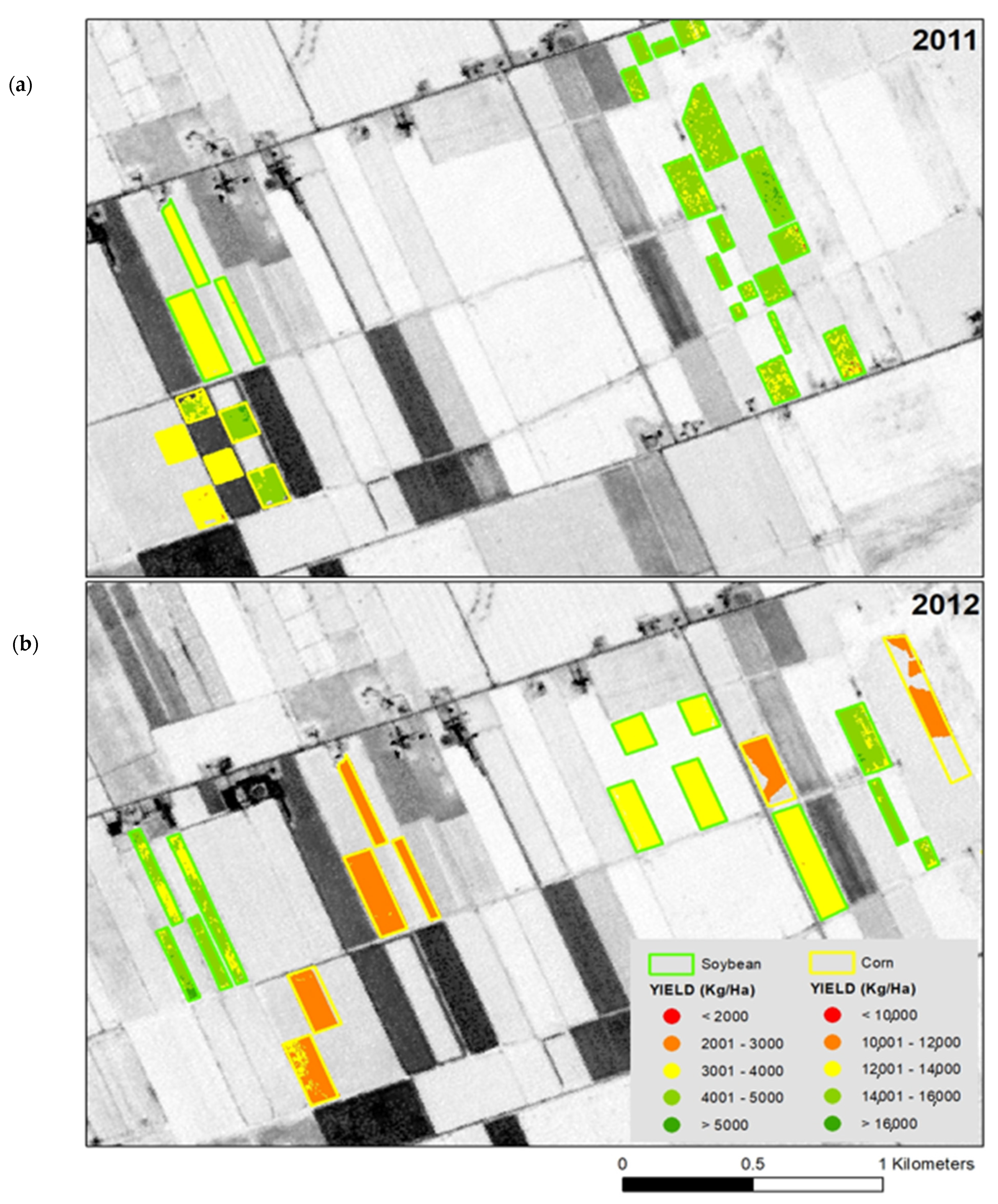
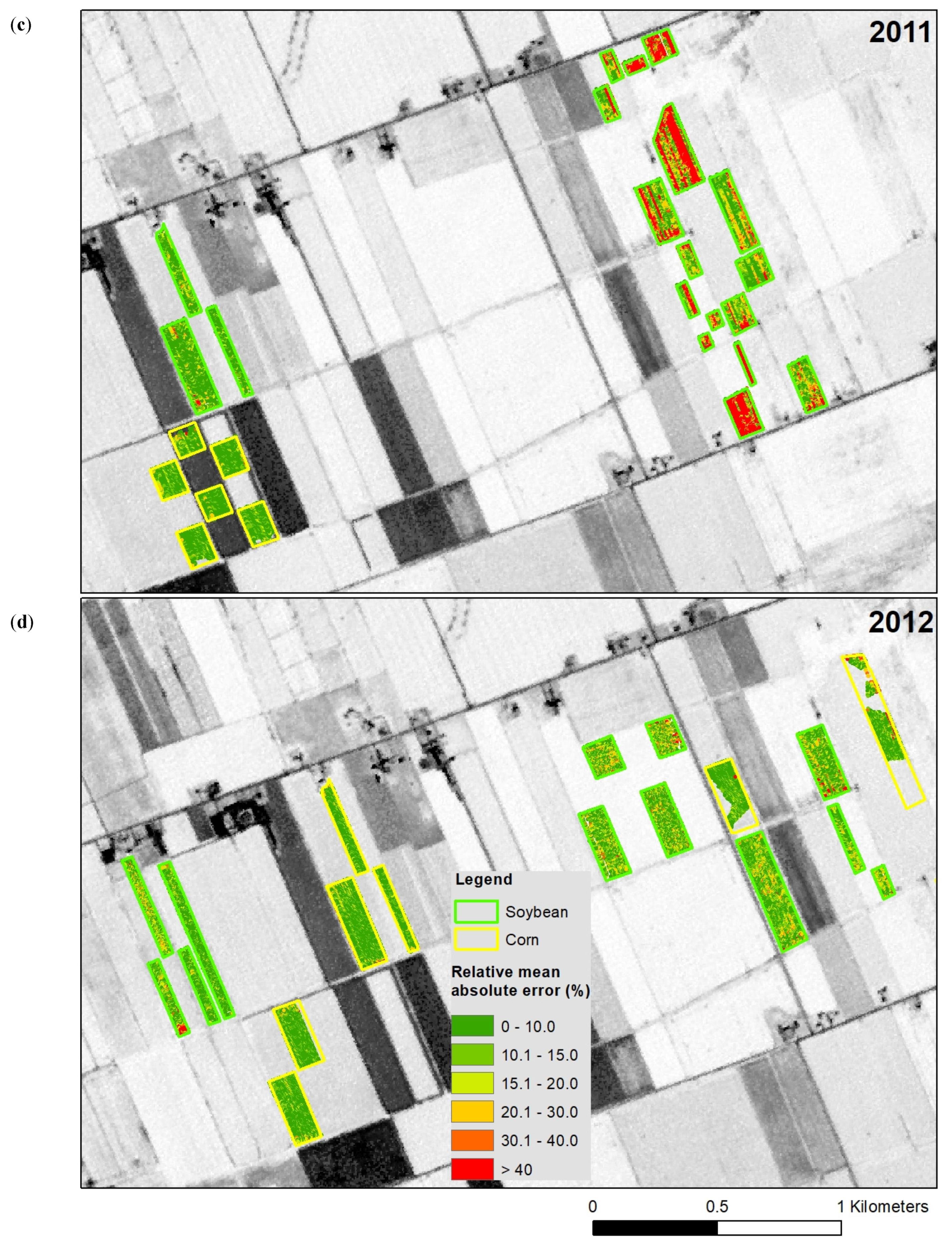
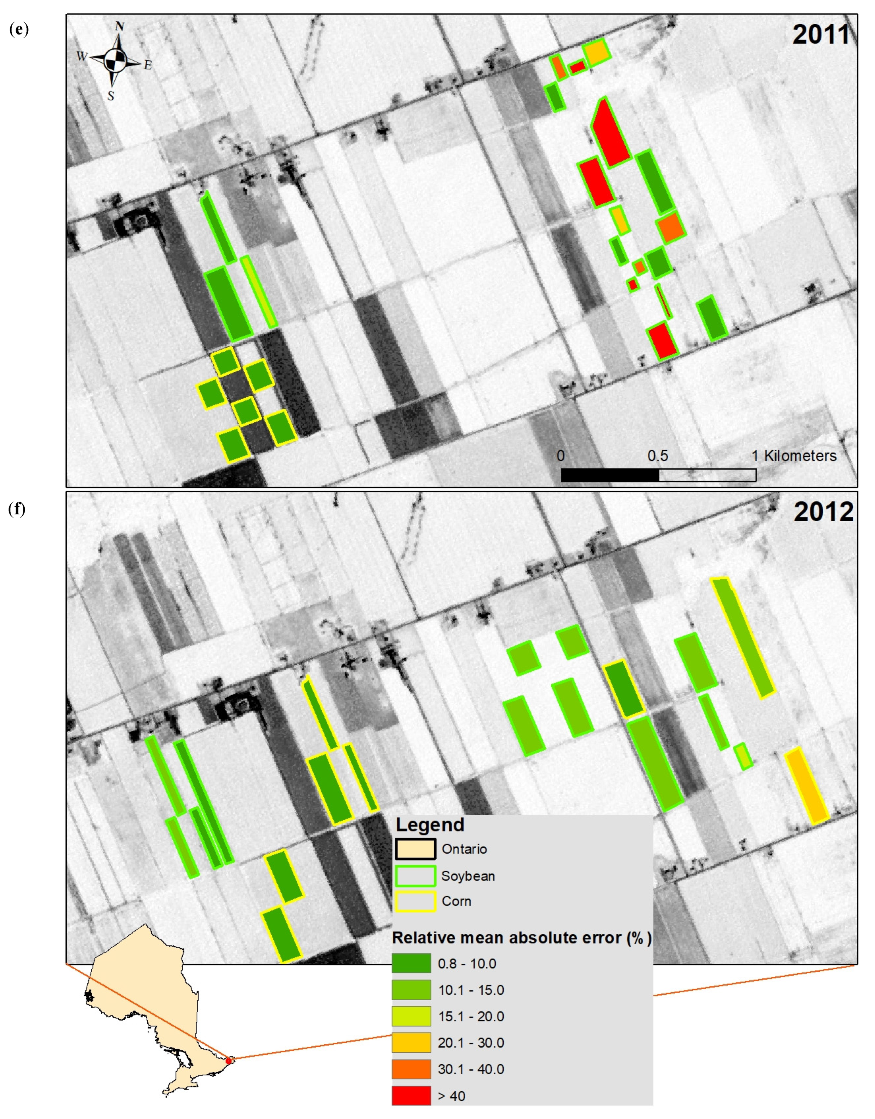
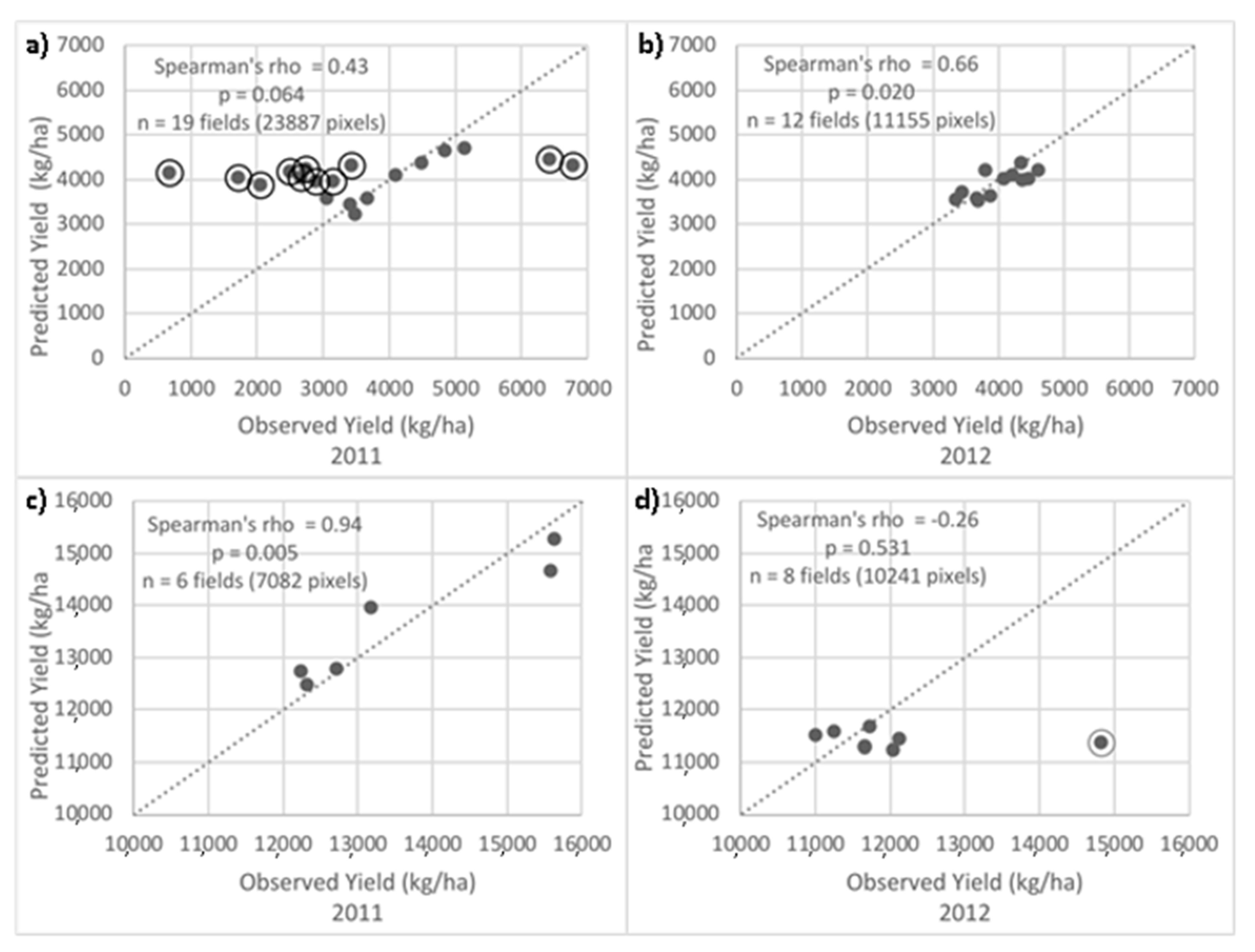
3.2. Predicted within-Field Corn and Soybean Yields

Crop-specific models that were trained and tested in the same year (PM004, PM006, PM019 and PM021 in Table 5, Figure 6a,d, Figure 7a–c) performed best according to the error analysis. In 2011, 100% of the corn fields had errors below 10%, while 42% of the soybean fields had errors below 15% (58% of the fields had errors > 20%). The observed soybean yield had high variability in 2011 where the average CV was 29% and about 15% of the fields had CV values below 10% (85% of the fields had CV > 20%, Figure 2). Observed corn yield variability was low in 2011 (CV < 10%). It is likely that the prediction error patterns reflected the observed yield variability in 2011. In 2012, both crop models performed well, as 75% of the corn fields had errors below 10% (87.5% of the corn fields had errors below 20%) and 100% of the soybean fields had errors below 20%.

Spearman’s rho correlations between the predicted and observed field yield measures ranged between 0.26 and 0.94, with the highest values for corn in 2011 and for soybean in 2012 (Figure 8; only for crop-specific models that were trained and tested in the same year). Performance results were consistent with approaches performed at the field [12] and regional scales [14]. Fiezal et al. [12] reported R² values between 0.05 and 0.77, with the best results for an ANN model to estimate corn yield based on the red wavelength reflectance values (16 images between May and September). Kaul et al. [14] evaluated the performance of ANN models for the prediction of yield at the state, regional and local level and reported R² values between 0.37 and 0.99 for corn, and between 0.66 and 0.91 for soybean. At these larger scales, Kaul et al. [14] identified the importance of weekly rainfall data. Rainfall can be considered uniform over the fields in our study area. At this scale, our results showed the importance of variables related to the canopy and surface structure, the SR index and slope, respectively. These structural variables contain implicit information on spatial patterns of soil, water and nutrient distributions [23], which can ultimately affect crop yield. In 2011, for example, the ANN models underestimated soybean yield in most of the eastern fields of the study area. The eastern fields have more variability in their micro-topography, as shown in the flow accumulation and slope maps (Figure 3 and Figure 4). The year 2011 was wetter than 2012 and 2016, which means that there was a greater mix of waterlogged and dry areas within the eastern fields (based on their higher variability in micro-topography). This may have affected the yield, but was not captured by the ANN models.

The error analysis showed low performance of the ANN models that were trained on both crop types combined (Models PM001 and PM015 in Table 5). Most of the test fields had errors above 20% for soybean and above 10% for corn (Figure 6). Models that were trained and tested in 2011 or 2012 were also used with predictor variables from 2011, 2012 or 2016. The prediction accuracy of these models was low, with RMAEs above 40% for most of the fields in all models (Figure 6; Appendix A: Table A1). The overall weaker performance of the ANN models that were trained and tested in one year, and then applied on other years could be attributed to:

(i)

differences in phenological development stages: the final models were developed based on images of specific dates. Even though the images of the application years mostly matched the model dates closely, actual crop development stages may not necessarily match.

(ii)

differences in image dates: 2016 image dates, for example, differed by up to 24 days from the image dates from the trained models, the largest errors were also observed in this year.

(iii)

differences in environmental and weather conditions: 2012, for example, was much drier than 2011.

Previous research [14,28] showed the importance of rainfall data during the growing season. Kaul et al. [14] suggested including weekly rainfall data as predictor variables for corn and soybean yield prediction, as monthly data were found inadequate for effective crop yield prediction. For field-scale studies, future studies can include the land surface water index (LSWI) or radar-derived soil moisture as a proxy for canopy and surface wetness.

Overall, the results indicate that the ability to predict within-field yield accurately during a growing season will partially depend on the ability of predictor variables to reflect:

• the crop type: future studies should explore potential variables for the development of crop-independent models or create crop-specific models.
• the canopy and surface wetness: information about water availability should be included (weekly data if possible).
• critical crop development stages: satellite images that match the critical crop stages should be included, which means that the phenological stages should be measured or estimated.
• field micro-topography: slope was an important indicator overall; future research should explore the inclusion of micro-topography metrics derived from slope data.
• differences in planting, spacing and management practices: the transferability of the models will depend on the homogeneity of crop management factors.

4. Conclusions

This study analyzed the relative importance of remotely sensed predictor variables for the estimation of crop yield and evaluated the performance of ANN MLP models for within-field corn and soybean yield predictions. Knowing which variables affect the end-of-season yield variability within a field is important for precision agriculture applications and decisions on agriculture practices. As most current studies within this domain have focused on large-scale approaches, this study brings information that contributes to methodological advancements and decision making at the farm level.

The results showed a greater importance of the structural variables (SR, slope, flow accumulation) and crop phenology for the prediction of end-of-season yield within corn and soybean fields.

When the models were trained and tested in the same year, the corn-specific model performed better than the soybean model: most of the corn fields had RMAEs lower than 15% for both years. For soybean, 42% of the fields had RMAEs lower than 20% in 2011 and 100% of the fields had RMAEs below 20% in 2012. The accuracy of the models reflected the measured yield variability: fields with a high measured yield variability also had large model errors.

References

1. Basso, B.; Liu, L. Seasonal crop yield forecast: Methods, applications, and accuracies. In Advances in Agronomy; Elsevier: Amsterdam, The Netherlands, 2019; Volume 154, pp. 201–255. [Google Scholar]
2. Noack, S.; Knobloch, A.; Etzold, S.H. Spatial predictive mapping using artificial neural networks. Int. Arch. Photogramm. Remote Sens. Spat. Inf. Sci. 2014, XL-2, 79–86. [Google Scholar] [CrossRef] [Green Version]
3. Weiss, M.; Jacob, F.; Duveiller, G. Remote sensing for agricultural applications: A meta-review. Remote Sens. Environ. 2020, 236, 111402. [Google Scholar] [CrossRef]
4. Verrelst, J.; Camps-Valls, G.; Muñoz-Marí, J. Optical remote sensing and the retrieval of terrestrial vegetation bio-geophysical properties—A review. ISPRS J. Photogramm. Remote Sens. 2015, 108, 273–290. [Google Scholar] [CrossRef]
5. Sun, C.; Bian, Y.; Zhou, T. Using of Multi-Source and Multi-Temporal Remote Sensing Data Improves Crop-Type Mapping in the Subtropical Agriculture Region. Sensors 2019, 19, 2401. [Google Scholar] [CrossRef] [Green Version]
6. Wang, H.; Magagi, R.; Goïta, K. Crop phenology retrieval via polarimetric SAR decomposition and Random Forest algorithm. Remote Sens. Environ. 2019, 231, 111234. [Google Scholar] [CrossRef]
7. Nevavuori, P.; Narra, N.; Lipping, T. Crop yield prediction with deep convolutional neural networks. Comput. Electron. Agric. 2019, 163, 104859. [Google Scholar] [CrossRef]
8. Johnson, M.D.; Hsieh, W.W.; Cannon, A.J. Crop yield forecasting on the Canadian Prairies by remotely sensed vegetation indices and machine learning methods. Agric. For. Meteorol. 2016, 218–219, 74–84. [Google Scholar] [CrossRef]
9. Yang, Q.; Shi, L.; Han, J. Deep convolutional neural networks for rice grain yield estimation at the ripening stage using UAV-based remotely sensed images. Field Crops Res. 2019, 235, 142–153. [Google Scholar] [CrossRef]
10. Gandhi, N.; Petkar, O.; Armstrong, L.J. Rice crop yield prediction using artificial neural networks. In Proceedings of the 2016 IEEE Technological Innovations in ICT for Agriculture and Rural Development (TIAR), Chennai, India, 15–16 July 2016; IEEE: Piscataway, NJ, USA, 2016; pp. 105–110. [Google Scholar]
11. Kuwata, K.; Shibasaki, R. Eestimating corn yield in the United States with MODIS EVI and machine learning methods. ISPRS Ann. Photogramm. Remote Sens. Spat. Inf. Sci. 2016, III-8, 131–136. [Google Scholar] [CrossRef]
12. Fieuzal, R.; Marais Sicre, C.; Baup, F. Estimation of corn yield using multi-temporal optical and radar satellite data and artificial neural networks. Int. J. Appl. Earth Obs. Geoinf. 2017, 57, 14–23. [Google Scholar] [CrossRef]
13. Li, A.; Liang, S.; Wang, A. Estimating Crop Yield from Multi-temporal Satellite Data Using Multivariate Regression and Neural Network Techniques. Photogramm. Eng. Remote Sens. 2007, 73, 1149–1157. [Google Scholar] [CrossRef] [Green Version]
14. Kaul, M.; Hill, R.L.; Walthall, C. Artificial neural networks for corn and soybean yield prediction. Agric. Syst. 2005, 85, 1–18. [Google Scholar] [CrossRef]
15. Fortin, J.G.; Anctil, F.; Parent, L.-É. Site-specific early season potato yield forecast by neural network in Eastern Canada. Precis. Agric. 2011, 12, 905–923. [Google Scholar] [CrossRef]
16. Kamir, E.; Waldner, F.; Hochman, Z. Estimating wheat yields in Australia using climate records, satellite image time series and machine learning methods. ISPRS J. Photogramm. Remote Sens. 2020, 160, 124–135. [Google Scholar] [CrossRef]
17. Jiang, D.; Yang, X.; Clinton, N. An artificial neural network model for estimating crop yields using remotely sensed information. Int. J. Remote Sens. 2004, 25, 1723–1732. [Google Scholar] [CrossRef]
18. Green, T.R.; Salas, J.D.; Martinez, A. Relating crop yield to topographic attributes using Spatial Analysis Neural Networks and regression. Geoderma 2007, 139, 23–37. [Google Scholar] [CrossRef]
19. Miao, Y.; Mulla, D.J.; Robert, P.C. Identifying important factors influencing corn yield and grain quality variability using artificial neural networks. Precis. Agric. 2006, 7, 117–135. [Google Scholar] [CrossRef]
20. Statistics Canada. Table 2.4 Principal Field Crop Production, by Province; Statistics Canada: Ottawa, ON, Canada, 2011.
21. Statistics Canada. Cropland in Ontario Grows Despite Fewer Farms; Statistics Canada: Ottawa, ON, Canada, 2017.
22. Sunohara, M.D.; Gottschall, N.; Wilkes, G. Long-term observations of nitrogen and phosphorus export in paired-agricultural watersheds under controlled and conventional tile drainage. J. Environ. Qual. 2015, 44, 1589–1604. [Google Scholar] [CrossRef]
23. Turpin, K.M.; Lapen, D.R.; Gregorich, E.G. Using multivariate adaptive regression splines (MARS) to identify relationships between soil and corn (Zea mays L.) production properties. Can. J. Soil Sci. 2005, 85, 625–636. [Google Scholar] [CrossRef] [Green Version]
24. Chlingaryan, A.; Sukkarieh, S.; Whelan, B. Machine learning approaches for crop yield prediction and nitrogen status estimation in precision agriculture: A review. Comput. Electron. Agric. 2018, 151, 61–69. [Google Scholar] [CrossRef]
25. Barth, A.; Knobloch, A.; Noack, S. Neural network—Based spatial modeling of natural phenomena and events. In Systems and Software Development, Modeling, and Analysis: New Perspectives and Methodologies; IGI Global: Hershey, PA, USA, 2014; pp. 186–211. [Google Scholar]
26. Garson, G. Interpreting neural-network connection weights. AI Expert 1991, 6, 46–51. [Google Scholar]
27. Bagg, J.; Banks, S.; Baute, H. Agronomy Guide for Field Crops: Publication 811; Ontario Ministry of Agriculture, Food and Rural Affairs (OMAFRA): Toronto, ON, Canada, 2009.
28. Kross, A.; Lapen, D.R.; McNairn, H. Satellite and in situ derived corn and soybean biomass and leaf area index: Response to controlled tile drainage under varying weather conditions. Agric. Water Manag. 2015, 160, 118–131. [Google Scholar] [CrossRef]
Figure 1. Overview of the study area. The fields (green polygons) located within the experimental micro watershed (blue outline). The background image is a RapidEye NDVI image. Not all fields were used within this analysis. The study area is located within the province of Ontario (Brown polygon, lower left), within Canada (upper left panel).
Remotesensing 12 02230 g001
Figure 2. (a) Overview of corn and soybean yield variability across fields in 2011, 2012 and 2016. (b) Overview of corn and soybean yield variability across fields in 2011, 2012 and 2016. Color classes refer to the coefficient of variation (CV) of the observed yield within each field.
Remotesensing 12 02230 g002aRemotesensing 12 02230 g002b
Figure 3. Slope where experimental fields were located during 2011 and 2012.
Remotesensing 12 02230 g003
Figure 4. Flow accumulation where experimental fields were located during 2011 and 2012.
Remotesensing 12 02230 g004
Figure 5. ANN multilayer perceptron network (MLP) for crop yield prediction.
Remotesensing 12 02230 g005
Figure 6. Overview of the performance of the ANN models, measured by the percentage of fields within different error ranges. Each stacked bar represents the percentage of fields within each RMAE % range (0–10; 10–15; 15–20; 20–30; 30–40; >40). Figures (ac) are results from models that were trained with 2011 data. Figures (df) are results from models that were trained with 2012 data. The model naming convention is as follows: PM001 = the model was trained and optimized for corn and soybean combined in 2011; PM004 = the model was trained and optimized for soybean only in 2011; PM006 = the model was trained and optimized for corn only in 2011. PM015 = the model was trained and optimized for corn and soybean combined in 2012; PM019 = the model was trained and optimized for soybean only in 2012; PM021 = the model was trained and optimized for corn only in 2012. The year indicates the application or test year, and the crop indicates which crop type’s yield was predicted. For example, PM006-2012-Corn = the model was trained with corn data from 2011, and applied on input variables from 2012 to predict corn yield in 2012.
Remotesensing 12 02230 g006
Figure 7. Overview of the results from the ANN models for 2011 (a) and 2012 (b). Results show the predicted crop yield of the models that were trained and tested with one crop, in one year. Overview of the results from the ANN models for 2011 (c) and 2012 (d). Results show the relative errors ((pixel error/field yield mean) * 100) of the models that were trained and tested with one crop, in one year. Overview of the results from the ANN models for 2011 (e) and 2012 (f). Results show the errors ((field mean error/field yield mean) * 100) of the models that were trained and tested with one crop, in one year.
Remotesensing 12 02230 g007aRemotesensing 12 02230 g007bRemotesensing 12 02230 g007c
Figure 8. Correlations among predicted and observed average field yield for soybean in 2011 (a) and 2012 (b) and corn in 2011 (c) and 2012 (d). Results show the correlations from the models that were trained and tested with one crop, in one year. The circled dots in panel (a) and (d) refer to the fields with an RMAE greater than 20%.
Remotesensing 12 02230 g008