GPR Spectra for Monitoring Asphalt Pavements


1
Department of Civil & Environmental Engineering, Universitat Politècnica de Catalunya, Campus Nord, Jordi Girona 1-3, 08034 Barcelona, Spain
2
Department of Strength of Materials and Structural Engineering, Universitat Politècnica de Catalunya, Campus Diagonal Besós, Barcelona East School of Engineering, EEBE, Av. Eduard Maristany, 16, 08019 Barcelona, Spain
*
Author to whom correspondence should be addressed.
Remote Sens. 2020, 12(11), 1749; https://doi.org/10.3390/rs12111749
Submission received: 8 April 2020
/
Revised: 23 May 2020
/
Accepted: 25 May 2020
/
Published: 29 May 2020
(This article belongs to the Special Issue Trends in GPR and Other NDTs for Transport Infrastructure Assessment)
Abstract
:Ground Penetrating Radar (GPR) is a prospecting method frequently used in monitoring asphalt pavements, especially as an optimal complement to the defection test that is commonly used for determining the structural condition of the pavements. Its application is supported by studies that demonstrate the existence of a relationship between the parameters determined in GPR data (usually travel time and wave amplitude) and the preservation conditions of the structure. However, the analysis of frequencies is rarely applied in pavement assessment. Nevertheless, spectral analysis is widespread in other fields such as medicine or dynamic analysis, being one the most common analytical methods in wave processing through use of the Fourier transform. Nevertheless, spectral analysis has not been thoroughly applied and evaluated in GPR surveys, specifically in the field of pavement structures. This work is focused on analyzing the behavior of the GPR data spectra as a consequence of different problems affecting the pavement. The study focuses on the determination of areas with failures in bituminous pavement structures. Results epitomize the sensitivity of frequencies to the materials and, in some cases, to the damage.
1. Introduction
1.1. Detection of Failures in Pavements
Traditionally, the presence of defects that affect pavement preservation to the greatest extent (moisture in the lower layers and lack of adhesion in the top pavement layers) is usually detected with deflection tests, although the study of the evolution of standardized indicators is also used, such as the International Roughness Index (IRI).
The basic parameter measured in the deflection tests is the vertical displacement produced in the pavement after applying a load. The result is the response of all the layers that make up the road structure, including the sub-grade. In addition, some measuring equipment, such as the Falling Weight Deflectometer (FWD) and the curviameter allow the deflection bowl generated by the load applied during the test to be interpreted, and the modulus of elasticity of the various layers that make up the pavement to be determined by means of back calculation [1].
Studies, Chea, and Martínez [2] for example analyse the adhesion between layers in a semi-rigid pavement showed that the deflection curve did not vary significantly, but that its first derivative and the radius of curvature under the loaded wheel could be used as a lack of adhesion indicator.
Another common problem, excessive moisture in the pavement layers, can affect its strength and thus reduce its useful life [3,4,5]. Recently, a study carried out in Torpsbruk (Sweden) demonstrated the applicability of the impact deflectometer in evaluating the effect of moisture in the unbound layers on the bearing capacity of a flexible pavement [6]. However, among its conclusions, the need to carry out a more intensive investigation that would allow the interpretation of the results to be improved was highlighted, so that environmental factors that affect the pavement response could be understood.
The work of Gedafa et al. [7] proposed a methodology based on the impact deflectometer using measurements made over eight years, with the aim of estimating the remaining life of a pavement depending on the deflections. Using a non-linear regression procedure, a very good fit sigmoidal relationship is determined that allows its remaining life to be predicted.
Various researchers have developed indices that consider the deflection value, the Structural Number (SN) being the most well-known [8,9]. Other indices, such as Surface Curvature (SCI), Base Damage (BDI), and the Base Curvature (BCI) were used to establish evaluation criteria for the granular layers treated with cement and for the bituminous layers [10,11,12].
The IRI test does not allow for the structural condition of a road to be defined, but its evolutionary analysis over time does allow its evolution to be studied [13]. Some researchers have developed models for predicting the Pavement Condition Index (PCI) based on the IRI. For example, Arhin et al. [14], through a functional classification (type of road: local, collector, arterial) and the type of pavement (flexible and rigid pavements), and based on data obtained in the district of Columbia over two years, found statistically significant results with a 5% margin of error. Park et al. [13] established a logarithmic relationship between the IRI and the PCI based on the results obtained from the acoustic monitoring of roads in nine North American states for a period of nine years. Dewan and Smith [15] related both indices for the streets of the San Francisco Bay Area, and developed a model that can be used to estimate vehicle operating costs directly based on deterioration identified in the pavement.
1.2. Geophysical Surveys in Pavement Assessment
As complementary evaluation of roads, geophysical surveys were tested and applied in many cases. These surveys provide a non-destructive analysis of the medium, based on the measurement of physical properties on its surface. The analysis of the values obtained for each one of those physical properties can be associated with models of the inner medium. Therefore, the properties and characteristics of the internal medium are deduced from indirect measurements. This type of studies presents benefits and limits. The benefits are mainly the quick data acquisition (in many cases data is acquired at a usual traffic speed) and the non-destructive character of the surveys, i.e., data acquired without damage the pavement. The limits are consequence of the indirect measurements, because the values of the measurement could correspond to different models of the medium. Therefore, in many cases, non-destructive techniques are applied combined with punctual drills or combining different NDT methodologies to avoid the vagueness and to obtain more accurate models. Several authors investigate the improvement of the results in case of different combinations of techniques, both in laboratory or in field tests. Capozzoli and Rizzo [16] compared GPR with resistivity tomography (ERT) and infrared thermography (IRT), obtaining promise results in the study of concrete, highlighting the different data obtained with each one of the techniques. The work of Lagüela et al. [17] demonstrated the ability of different techniques: GPR, IRT and laser terrestrial scanning (LTS), in the assessment of paving, showing the different damage observed with each one of those methods. A revision of the state-of-the-art in the assessment of pavement structural conditions, comparing the results in the estimation of thickness and moduli of different layers can be found in [18]. In many cases, the analysis of the pavement conditions are evaluated by using GPR and falling weight deflectometer (FWD) [19,20,21]. A wide revision of fundamentals and applications of NDT and geophysical surveys in the assessment of structures and infrastructures can be found in [22,23]. The most widely applied techniques are seismic methods, IRT, ultrasonic tomography, and GPR. Seismic surveys are widely used in pavement assessment. The method consists of the measurements of the pavement response to vibrations that are produced by falling weights. Other methodology used in the pavement tests is thermography, based on the detection of infrared radiation. Several studies indicate that this technique is appropriate to detect pavement defects, differences in compaction, cracking, and delamination [24,25,26]. Ultrasonic tomography has been also applied to detect cracks in concrete pavements [27,28]. The shallowest layers (asphalt binders) have been analyzed in some cases by using acoustic emission in order to detect incipient cracking [29,30]). GPR is other widely used technique in the assessment of pavements. Many of those techniques are applied in combination with other methodologies and, in all cases, with coring in specific points.
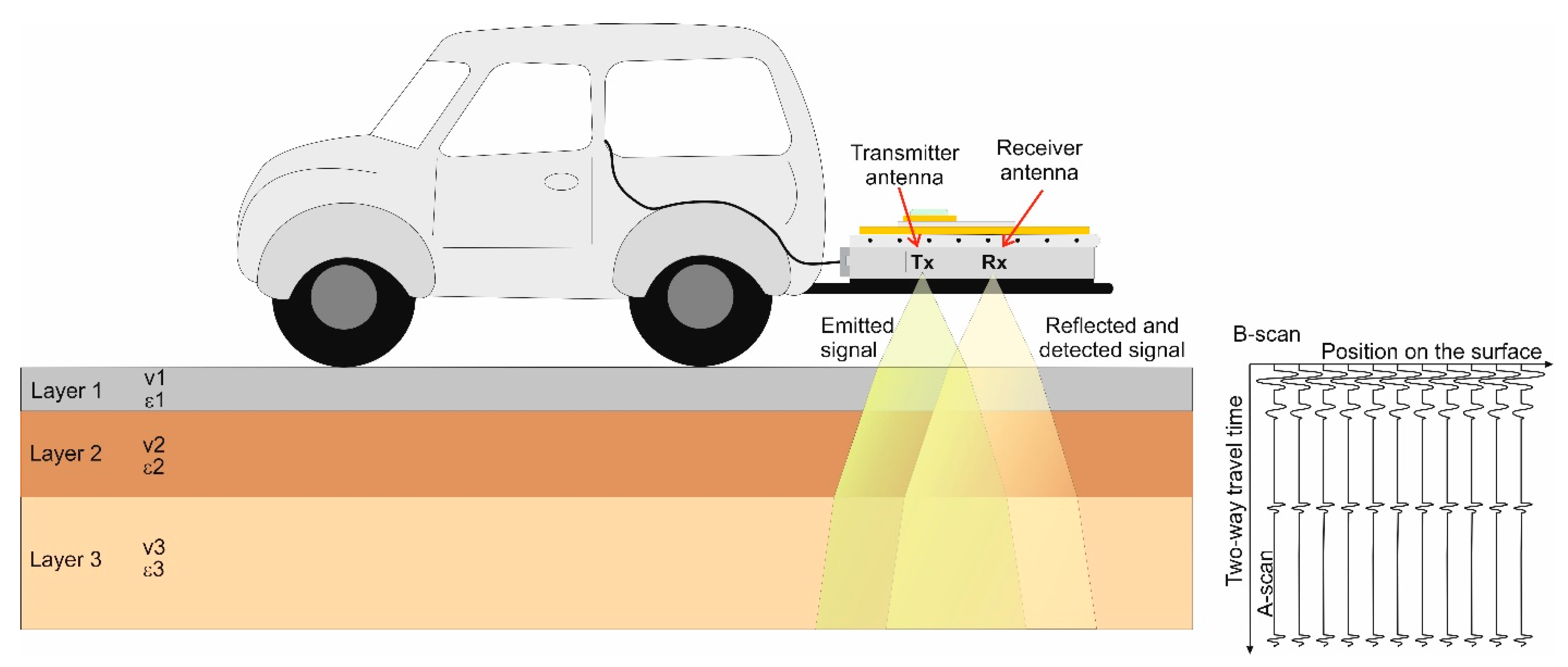
The GPR technique consists of the emission and reception of electromagnetic ultra-wideband frequency waves, in the range of microwaves and radiofrequencies. A transmitter antenna generates and transmit the signal that propagates through the medium. The existence of electromagnetic discontinuities produces partial reflection of the energy that propagates back to the surface of the medium. A receiver antenna detects that reflected energy (Figure 1). Each one of the recorded pulses is called A-scan, and the collection of these individual traces is the B-scan. In many road assessment, GPR usually collects one trace each 20 or 25 cm.
The first applications of GPR in pavement assessment were focused on the detection of layers, determining their thickness [31,32,33,34]. Later, the technique was applied to the detection of cracks [34,35,36,37] and to the analysis of properties and parameters of the asphalt and other layers, based on the estimation of their dielectric permittivity [38]. The method was also applied for moisture and infiltration control [39,40]). Even though GPR is applied to determine damage in pavement, distinguishing between specific details or causes is difficult because diverse anomalies could produce similar response in the GPR signals. For example, some researchers showed that non-destructive technologies are not able to identify debonding between asphalt layers because of an inadequate tack coat execution. However, GPR can be used to detect this distress when moisture is trapped in the interface [41,42]. In addition, some researchers discuss the ability of non-destructive technologies to detect an inadequate tack coat execution [41]. However, it was shown that GPR can be used to detect the distress caused when pavement layers are debonded, which can be a consequence of a deficient tack coat application [43]. Moreover, the document published by RILEM Technical Committee 241-MCD (RILEM State-of-the-Art Reports) considers this option: “techniques for detecting debonding using Ground Penetrating Radar have also shown promise” [44]. Also an investigation about the use of GPR to characterize changes in geometric and dielectric properties of the tack coats has been carried out and results prove the suitability of the technique proposed [45].
1.3. Application of GPR in the Detection of Road Failures
Currently, many pavement studies are complemented with non-destructive tests (NDT), being GPR one of the most extended methods (e.g., [46]), in many cases applied in combination with other NDT techniques such as thermography. GPR assessment provides an evaluation of defects that are located by analyzing the anomalies in the images. This type of analysis started to be applied in the 1980s to locate voids under the pavement layers [47], with varying degrees of success (e.g., [48,49]).
The technique is usually based on the determination of the electrical permittivity in the various stretches of road. This parameter depends on the materials that make up each medium, and it substantially determines the speed of propagation of the electromagnetic wave. In dielectric media, the relationship between the signal speed () and the relative dielectric permittivity () is determined by means of Equation (1).
where is the speed of propagation of the electromagnetic wave in free space (approximately 30 cm/ns). The limits between the different materials are detected from the reflection of the signal that occurs when there is a significant contrast in the dielectric constant of the media. The two extreme values considered for are those for water (approximately 81) and those for air (approximately 1), while the other materials that usually form part of the studied media have constants between 2 and 30 [50]. In particular, composite materials with bituminous binders usually have values that vary between 2 and 12 [51,52]. The total thickness of each layer () is calculated as the product of the propagation time of the wave reflected at the base of the layer (Δt) divided by two, and its average propagation speed (v), as defined in Equation (2).
Equation (2) shows that the calculation of h includes an estimation of εr, so the speed of propagation of the signal can be determined. Although sometimes values already defined in the existing literature are considered, in other cases they are determined experimentally by analyzing specific cores and comparing them with the propagation times recorded in the area. Occasionally, a comparison will also be used between recorded amplitudes and signal amplitudes obtained in a prior calibration on metal plates. The entire energy incident on a metal plate is reflected; therefore the reflection coefficient in this case is one. By comparing the reflection coefficients in the ideal case (calibration on metal) and for a real surface, a permittivity value can be defined for the outermost surface of the layer by means of a relationship between the amplitudes (Equation (3)).
where A0 is the amplitude of the wave reflected from the top of the pavement, and. Am is the amplitude of the wave reflected on a metal plate located at the same distance from the antenna as the top of the pavement.
Test standard ASTM D4748 [50] states that the resolution of the GPR is sufficient to measure a minimum thickness of 40 mm with an accuracy of 5 mm. Some researchers have verified that the error made on measuring thicknesses is comparable to that made on direct measurements on cores (e.g., [32,52,53,54]).
1.4. The Frequency Spectrum
There are few works based on the analysis of the frequency spectrum of the GPR reflected signals. Some of the first studies used the frequency only to distinguish the antenna, determining differences in wave velocity [63] and in the absorption [64] depending on the antenna frequency. Frequency analysis was also included in laboratory resolution studies [65], comparing the frequency spectrum in air and in different media, which reduce the center frequency, the amplitude, and the bandwidth. Some studies focused on the detection of changes in water content in concrete determine also that the center frequency and the bandwidth decreases as water content increases [66,67], even though the main objective was the analysis of the wave amplitude, analyzing in some cases the spectra amplitude attenuation depending on the water content [68]. The analysis of the spectrum behavior combined with backscattering was also applied in the study of shallow geology to detect seasonal subterranean streams, differentiating between active and non-active streams [69] and in the study of compaction and moisture in sandy loam [70]. Further evaluations studied the propagation of GPR signals in unsaturated ground using the Rayleigh dispersion and confirmed that the frequency of the waves changed depending on the moisture content: the maximum amplitude observed moved to lower frequency values as the water content increased [61]. The changes in the GPR spectrum were also observed in studies evaluating the hydration phenomena of Portland cement as it passed from the fresh to hardened state by measuring the changes in the GPR signal spectrum over 90 days and recording the variations in the maximum amplitude values of the frequency spectrum [62]. It was also observed that the amplitude increased with the age of the concrete, confirming the relationship observed in other materials. Laboratory experiments with soils denote also that the clay content affected the shift and peaks of GPR frequency spectra, obtaining peaks at lower values as clay content increases [71,72].
Similar line of analysis, applied to the assessment of the pavement base, was focused on the study of water content, providing promising results and showing that the shift and peaks of the spectrum could most likely be and indicator that help in the mapping of spatial soil moisture variability [60,73]. The spectrum is also sensible to clay content in the pavement base, and several studies point to the possibility of using the peaks displacement to detect changes in clay content [74]. The work of Pedret et al. [42] analyses a section of flexible pavement by evaluating the changes in the spectrum according to the thickness of the bituminous mixture layers, the moisture and the detachment between layers. Based on the variations observed in the bandwidth and in the amplitude of the frequency spectrum maximums, the use of GPR is proposed to define stretches of road in accordance with the parameters observed in the frequency spectrum.
1.5. Study Objectives
The preliminary tests in selected areas show an interesting correlation between the form of the amplitude spectrum and the structural condition of the pavement [42]. However, in these first analyses, the records were studied at certain points by evaluating individual traces. The analysis of individual traces could introduce errors as on occasions sporadic alterations can occur in a single trace or a few traces due to factors external to the study. For this reason, and based on the results obtained, the possibility was considered of analyzing different stretches by characterizing them with an average spectrum for each one. This would reduce the effect of anomalous traces and produce a more accurate and reliable result. That previous work [42] demonstrated the existence of changes on the frequency pattern associated with the thickness of the layers, being the peaks of the spectrum moved to the lower frequencies in the case of higher thickness. Those results pointed to a relation between the different zones of the spectrum and the contacts between materials and, in some cases, with debonding between layers.
These results were complemented with more detailed tests and further processing, including the average of traces in the same place. Therefore, the purpose of this work is, therefore, to develop and analyze a possible methodology that can be applied to the analysis of the pavement which is based on the study of the frequencies of the GPR records, based on a comparative analysis of the frequencies that would enable possible structural changes and the existence of damage to be identified. For this, the results of an exhaustive prospection on a pavement are studied. The prospection was focused on determining changes in pavement sections and on the effect due to voids and moisture.
2. Methodology
To achieve the objectives of the work, a section of motorway was selected with known pavement design cross-sections and conditions. A prospection campaign with GPR was carried out in this sector. Previous deflection and surface roughness test results are available for the same sector, as well as information on the traffic carried.
The GPR records are used to carry out a comparative study between the spectra of the recorded signals measured in various areas of the motorway. This comparison allows the small alterations observed in the form of the spectrum to be evaluated with respect to a reference spectrum.
The motorway chosen for the study is one of the main accesses from the north of the metropolitan area of Barcelona with an annual average daily traffic (AADT) of 15,000 with 10% heavy vehicles, it was put into service in 2006. It was chosen because in a short stretch (about 7800 m) three types of well-defined and known design cross-sections coexist. Each one of the cross-sections represents one of the best-known pavement typologies [75].
A total of 7800 m is studied which ensures the geographical proximity of each one of the records. Therefore, it is considered that there are no local climate or traffic density changes that affect the test, as the length of the analyzed stretch is short.
The sectors are defined taking into consideration the three existing design cross-sections over the total analyzed stretch. For each cross-section, three subsectors of length between 700 m and 1000 m are considered depending on the state of preservation of the pavement. The information used to define the subsectors was obtained from the previous deflection and IRI tests.
The analysis is carried out by comparing the frequency spectra of the radar records, which are characteristic of each subsector, and evaluating the influence of the design and the state of preservation of the pavement.
The standardized CDA (Cumulative Difference Approach) segmentation method has been used, as set out in the AASHTO (1986) [76] guide, for delimiting the subsectors. The criteria used consist of delimiting the changes of slope of the cumulative deviations of the set of values recorded in the deflection measurements. This ensures sufficient homogeneity in the characteristics of each one of the subsectors. Table 1 shows the three sectors and the nine subsectors considered, their length and segmentation in accordance with the deflection and roughness test results.
2.1. Design Cross-Sections Considered
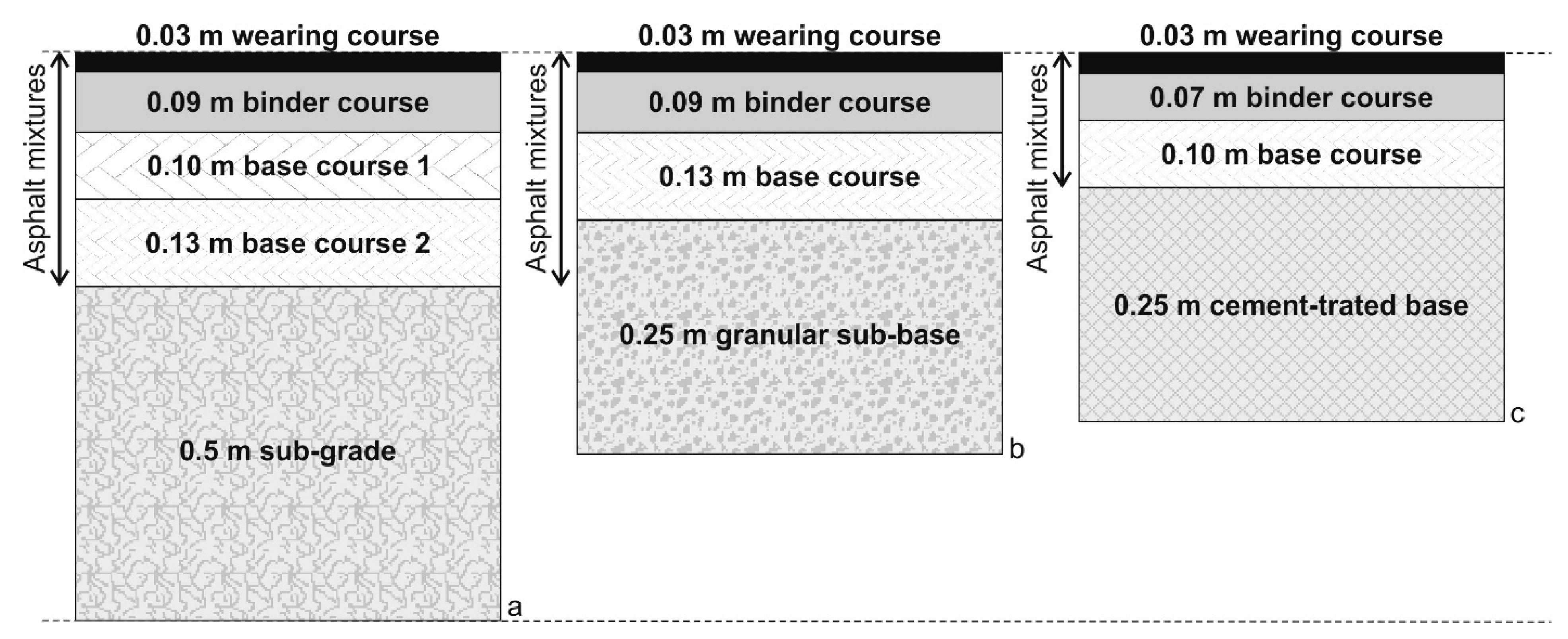
The three design cross-sections of the stretch of road studied (called A, B, and C) are shown in Figure 2. Cross-section A shows a full depth type pavement with a very thick layer of bituminous mix on a base of compacted soil forming the sub-grade. The design cross-section of the pavement is made up of different layers of asphalt mix with a total thickness of 35 cm (Figure 2a). Cross-section B is a flexible pavement. The design cross-section is made up of several bituminous mix layers of 25 cm thickness in total, on an untreated granular base of 25 cm (Figure 2b). Cross-section C is a semi-rigid pavement. The design cross-section is made up of a series of bituminous mix layers with a total thickness of 20 cm on a cement-treated granular base of 25 cm (Figure 2c).
2.2. State of Preservation of the Studied Sectors
The initial definition of the nine subsectors of the studied stretch of road, taking into consideration their construction characteristics and state of preservation, was made based on the results of the deflection and roughness tests using cumulative frequency histograms. The presented values correspond to all the measurements carried out on each one of them.
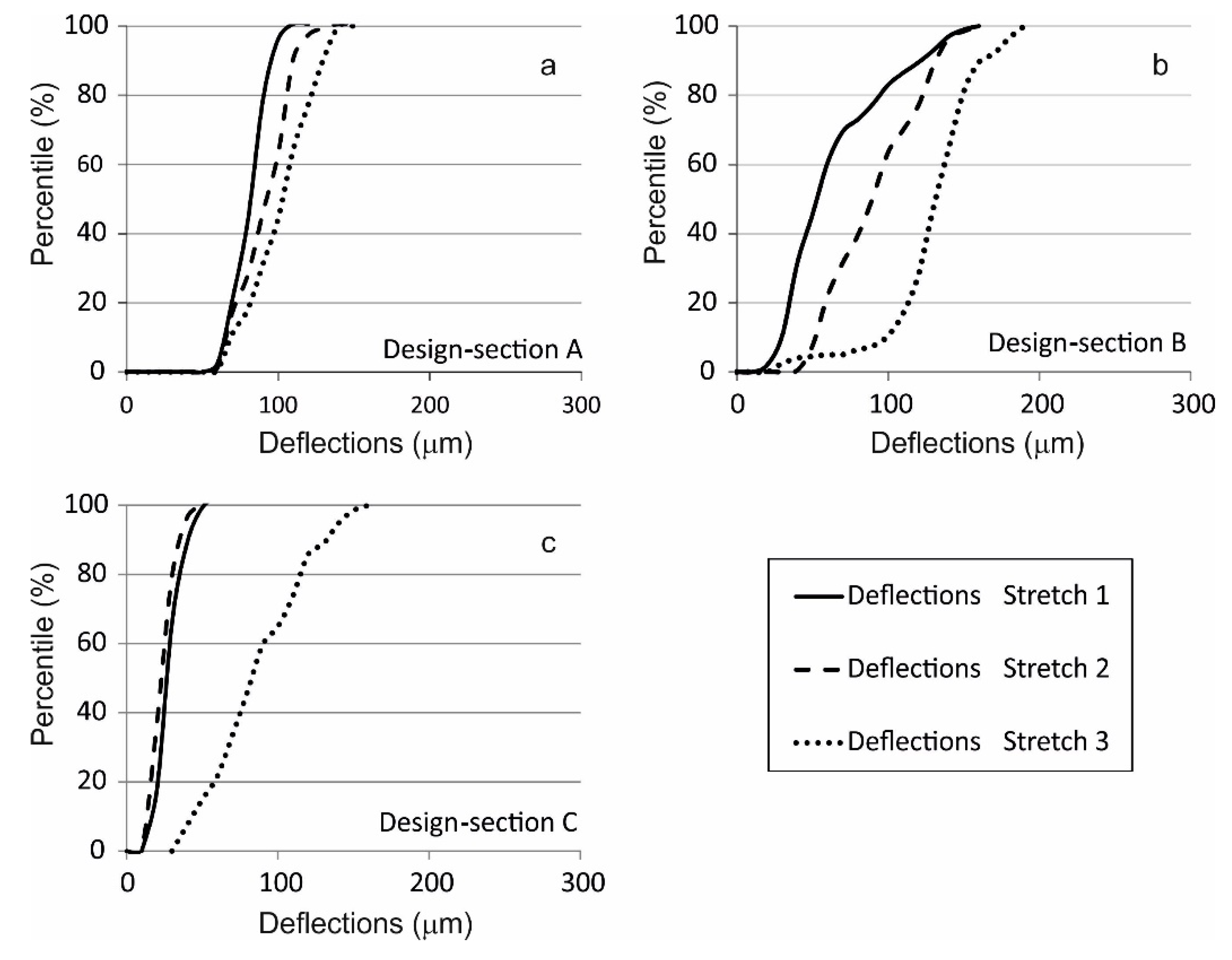
Figure 2 shows the resultant values of the deflection measured with the Lacroix deflectometer device [77] in each one of the considered subsectors. The continuous line and discontinuous line graphs in Figure 2 show the subsectors in best and intermediate conditions, respectively. The dotted line graphs in Figure 2 show the subsectors in the worst conditions. The deflections obtained in cross-section A (Figure 2 and Figure 3) showed low values due to the thickness of the combined bituminous layers which gives the system a high rigidity.
The deflections obtained in cross-section B (Figure 2 and Figure 3) show a large range of conditions. A subsector can be seen in very good condition with low deflections, a second subsector in reasonable condition, and a third subsector that has very few areas in good condition. In the subsector in worst condition, there are practically no points under the 100 µm value.
In the deflections obtained in cross-section C (Figure 2 and Figure 3), two of the subsectors are shown to be in very good condition while the third is in worse condition. The different zones, depending on the deflection results were called D1, D2, and D3, indicating increasing levels of deflection, although the thresholds are low in all three cases
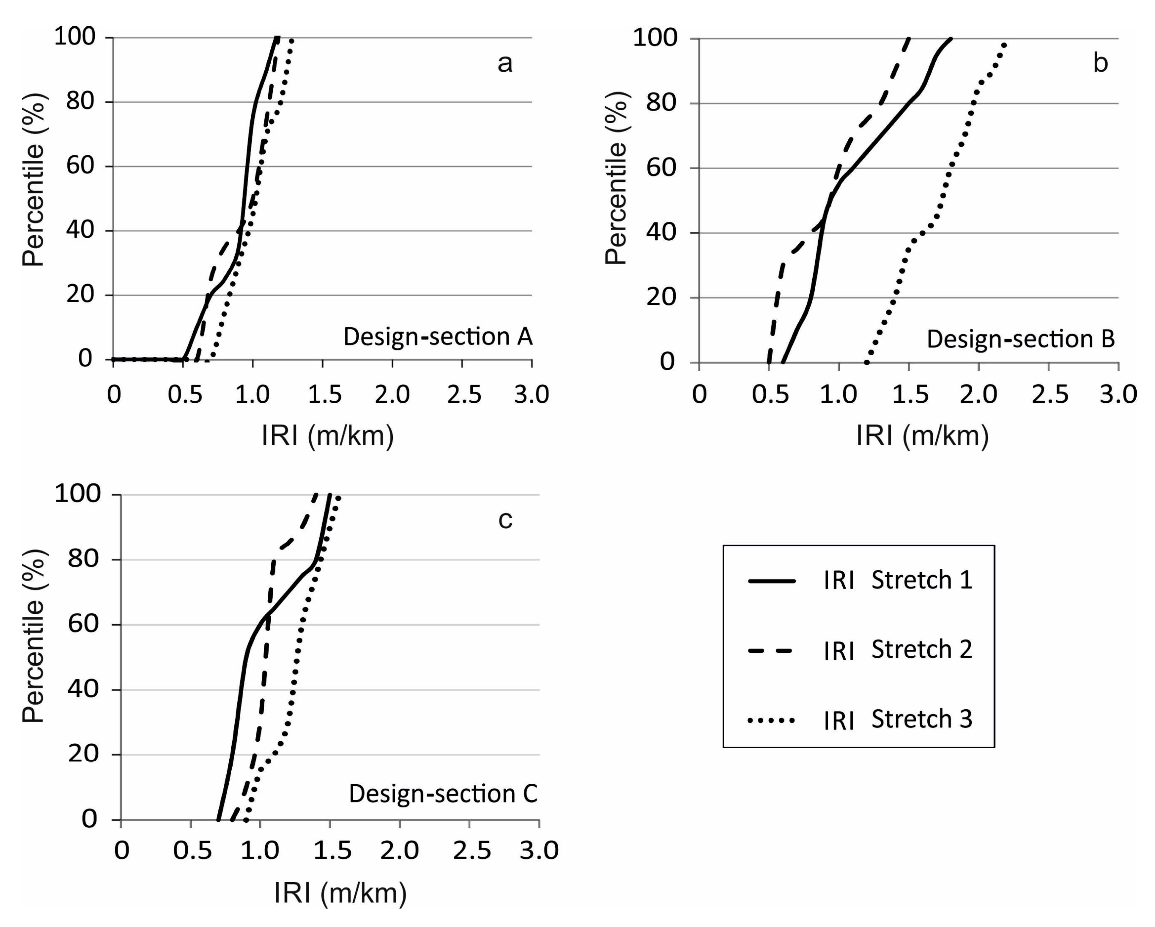
Figure 4 shows the pavement roughness results, measured with the IRI index, for the three pavement cross-sections.
Considering the 50 percentile of the set of values, a consistency can be seen in the deflection results, that is to say, the stretches in best condition also usually show a better IRI, even though there is no direct correlation of values.
The surface roughness test has only been taken into consideration in this study as a criterion for assessing the preservation condition in stretches where it is considered that the deflection test is not sufficient to provide the classification, as values are obtained within the same order of magnitude.
2.3. Methodology Applied for Evaluation by GPR.
Once the subsectors into which each sector is divided are defined (by a characteristic structural cross-section), the inspection campaign with GPR was carried out on each one of them continuously and at an adequate speed (between 60 and 80 km/h) so as not hold up the traffic, a trace was taken every 25 cm with a sampling frequency of 15,000 MHz.
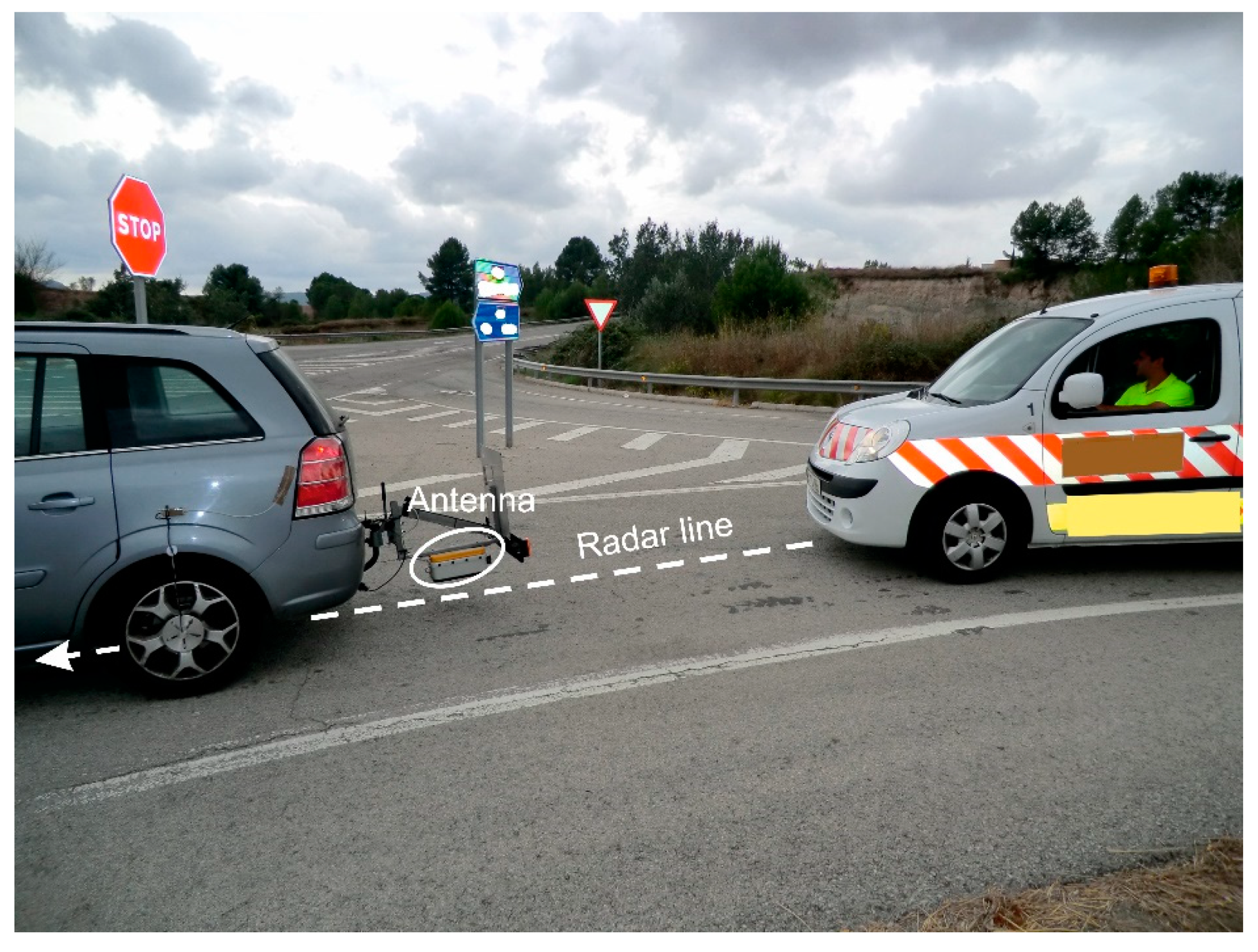
The profile data acquisition was carried out continuously in the center of the right-hand lane which carries mainly heavy vehicles (Figure 5). For the test, an antenna with a central frequency of 900 MHz was used after prior calibration. For this, the direct and reflected wave were analyzed after it was propagated through the air.
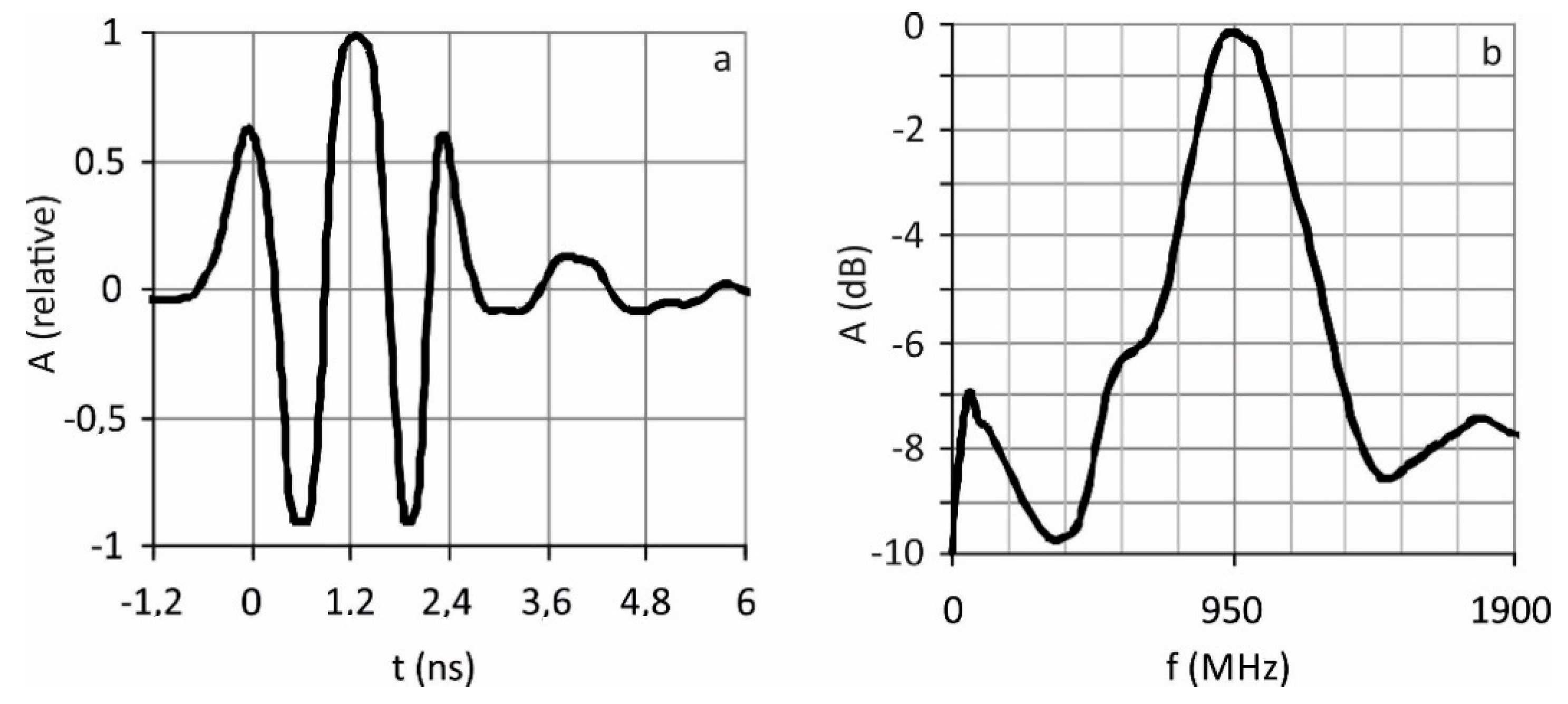
The calibration results are shown in Figure 6, which shows its pulse form and its frequency spectrum. It can be seen that the wave has a central frequency (f) at around 950 MHz, a bandwidth (BW) of about 350 MHz measured at −3 dB and a period of approximately 1.2 ns.
2.4. Calibration of the Signals in Known Media
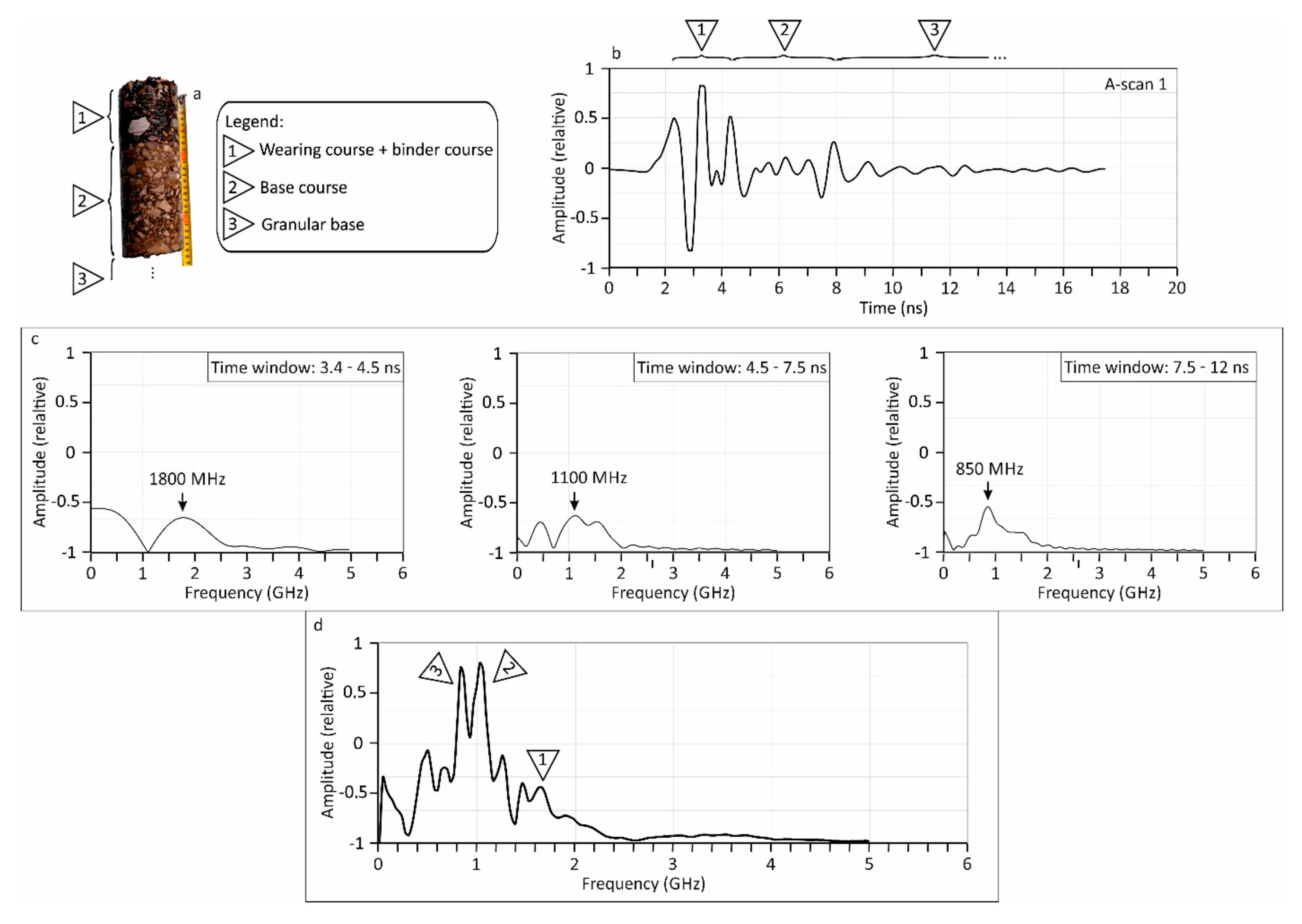
Before carrying out the signal acquisition, GPR data was acquired in specific and known zones, and the results were analyzed in order to determine propagation velocities and possible correlations between the form of the frequency spectrum and the different characteristics and pathologies of the pavement. The results of those preliminary tests are analyzed and discussed in [42]. Further contrast images were also acquired in the motorway studied in this work, always in points at which cores were obtained, in parts without visible damage. Figure 7 shows the core and the radar images obtained in one of these contrast tests, in kilometric points (KP) without construction defects and visible damage.
The road cross-section observed in the core (Figure 7a) presents three main layers: an upper part composed by wearing and binder courses, a second layer corresponding to the base course, and the end of the core is placed in the contact with the granular base. Therefore, the structural cross-section of the core shows two asphalt layers and the contact with the granular base. The top asphalt layer comprises both the wearing and binder course layers. Underneath there is a bituminous base layer spread over a granular base.
The wave velocity was obtained at each layer by comparing the two-way travel time in the A-scan to the thickness observed in the core (Figure 7b). This trace shows the correspondence between the number of transitions between layers and the number of amplitude maximums of the wave due to the reflection of the signal at each discontinuity. The maximum located at a time around 4.3 ns corresponds to the transition between the bituminous base and the granular base. The peak located around 1.5 ns corresponds to the transition between the two bituminous mix layers, and the initial peak located at 0 ns corresponds to the transition between the air and the pavement. Comparing those times with the core layers thickness, an average velocity of about 11.4 cm/ns is obtained, corresponding to the shallowest layer (wearing and binder courses), and a wave velocity of about 8.7 cm/ns in the base course.
The spectrum of the A-scan was compared to the spectrum obtained in air. A detailed analysis of the frequency of the received signal also shows variations in its maximum amplitude frequencies that appear to correspond with the different structural discontinuities of the pavement [42]. In general, the amplitude of the spectrum diminishes, and several peaks appear at frequencies of about 850 MHz, 1.1 GHz, and 1.3 GHz (Figure 5). These three maximum values are associated with three layers observed in the core and in the A-scan. This spectrum represents the frequency distribution of the received signal. The graph shows that the two main peaks are placed around 950 MHz. Each one of these corresponds to the two predominant materials in the environment: The asphalt mix of the base (frequency higher than 950 MHz) and the granular base (frequency lower than 950 MHz). Those results are considered to be contrast data to be compared with the radar data acquired in different sectors with a different damage degree.
The material of the medium through which the wave propagates, acts as a low pass filter. For this reason, the result obtained is logical as the layers located nearest the surface appear to be represented by the maximum amplitudes in the frequency spectra. In the spectrum shown in Figure 7c, the maximum indicated as 1, located at about 1200 MHz, represents the combined wearing and binder courses, which are the uppermost layers. The second maximum (2), at about 1000 MHz, represents the base mix. Finally, the maximum indicated as 3, located at about 900 MHz, corresponds to the granular base.
2.5. Signal Processing
(a) Processing A-scan—Signals recorded in each one of the stretches were processed to correct baseline deviations of the records, moving the zero offset of each A-scan with a dewow filter [78]. Other filters were not applied to the traces. This processing is usual in pavements GPR surveys to remove the low frequency and the down-shifting, but including in many cases a gain function application (e.g., [25,34,79]). Those filters were not used in this case because the study was focused on the spectrum analysis. The frequency spectra were obtained by means of a Fourier transform. Subsequently, they were smoothed by using a low pass filter with a cutoff frequency of 6 GHz, so the maximum values obtained could be more clearly seen.
(b) Processing B-scan—The analysis of individual trace spectra can provide results that are unrepresentative of the pavement studied when the study is carried out on randomly selected A-scans chosen from B-scans. An anomalous element on the surface, such as an irregularity in the ground or a waterlogged area, can affect a trace or a small and limited set of traces. If one of them is selected in the pavement analysis, the result may be due to external elements and will not show the average characteristics of the analyzed stretch of road.
For this reason, all the A-scans obtained over the same subsector (previously determined based on IRI and FWD data) have been averaged. In the resultant average trace, the effects due to small elements and surface factors are minimized, while those elements that are nearly constant throughout the subsector are represented. In this way, a record is obtained with very little noise that can be considered characteristic of the stretch. After applying the Fourier transform to this averaged trace, the resultant spectrum characteristics depends on different more general aspects of the pavement, such us number of layers, thickness of the layers, state of preservation and moisture. The shape and characteristics of the spectrum are determined by some of those aspects of by the combination of several of them. It is not possible to distinguish the causes of the changes. Hence, it is crucial to differentiate between types of pavement and state of preservation in order to associate with less uncertainty each GPR anomaly to the different pavement characteristics. The previous inspection is based on IRI and FWD, and determines each one of the subsectors identifying their constructive typology and by their degree of preservation.
3. Results Obtained
To check the sensitivity of the proposed frequency analysis-based method, a comparative study of the obtained frequency spectra is carried out, in accordance with the considered stretches of the road. Therefore, the study compares possible variations in the spectrum by averaging the results obtained in a particular road subsector. The comparison of these spectra with the IRI and FWD data and with specific cores shows the effect due to the typology of the construction cross-section and, for a same cross-section typology that is due to the different integrity levels.
3.1. Effects of Construction Cross-Section Variations
In the first test, the behavior is studied of the signal frequency spectrum in the case of variations in the pavement structure.
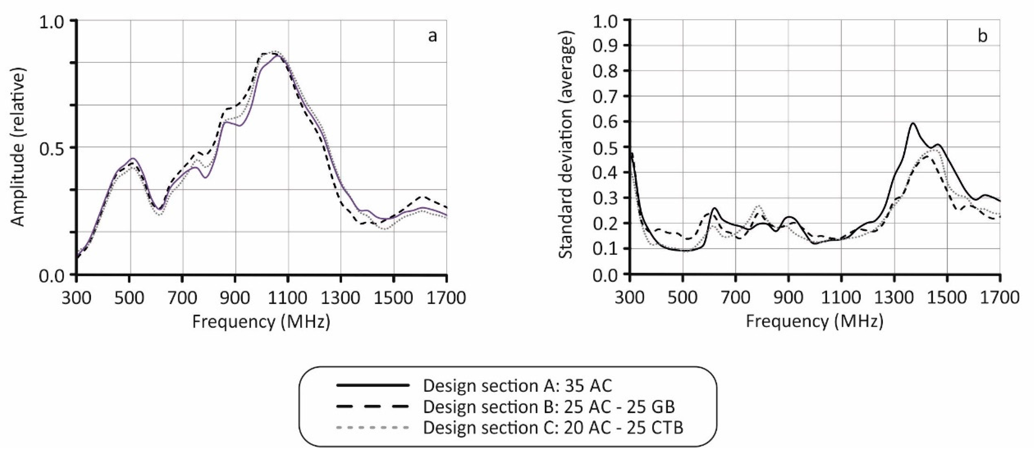
To avoid the effect due to the state of preservation of the pavement on the spectrum, a comparison is only made on those stretches in best condition. The known stretches with different cross-sections are analyzed (A, B, and C in Figure 1). Figure 6 shows the results obtained, averaged for each selected subsector. Standard deviation obtained for each one of the averaged spectra in the zone of interest (near 950 MHz) is approximately between 10% and 20%.
The graphs in Figure 8 are characterized by a minimum or an inflection at 950 MHz. The spectrum that has a minimum at these frequencies shows behavior similar to that of the spectrum in Figure 5. However, on comparing the three cross-sections in Figure 6, a notable change in this behavior is apparent for each section. Depending on the section, the minimum becomes a change in the curve inflection.
The maximum corresponding to the frequency above 950 MHz, associated with the combined bituminous mix layers, remains almost unchanged in the three design cross-sections. However, the same is not true of the maximum associated with the granular and cement-treated bases, located at about 900 MHz. At a lower frequency, the amplitude of this maximum reduces considerably in the type A structural cross-section, the amplitude is higher in the type B cross-section and higher still in the type C cross-section.
The amplitude differences of the maximums of the spectra associated with the bases in cross-section A and B are small, and could be due to the depth of each layer, as the depth of the granular base in cross-section A is, on average, at about 35 cm, while in the case of B, it is at about 25 cm. As B is closest to the top surface, it is logical that the amplitude of the maximum associated with the granular base is greater, as the high frequencies have not been attenuated to the same extent by the effect of the media.
The case of cross-section C is different, as the maximum that corresponds to the cement-treated base layer is very pronounced, and the difference of depth of this layer with respect to cross-section B is small (on average, about 5 cm). Therefore, a possible explanation of that observed in the record is the effect of the cement-treated base layer on the signal. This would indicate that this layer has electromagnetic characteristics that are sufficiently different from the other materials, so that changes in the frequency content of the records can be detected.
Although a similar case was analyzed [35] in preliminary studies, there are no exhaustive studies on the frequency behavior of GPR signals obtained in a pavement with a cement-treated base layer.
The results can be evaluated based on the composition of these types of layers. Table 2 shows the physical characteristics (relative dielectric permittivity and electrical resistivity) of asphalt mixtures, conventional granular bases, and cement-treated bases [80]. This data is obtained measuring by a 900 MHz shielded antenna and a distance of 20 cm above the surface pavement.
The dielectric permittivity and electrical resistivity of the asphalt mixtures are more similar to those of a conventional granular base than those of a cement-treated base.
3.2. Effect of Variations of the Pavement Integrity Condition
The analysis was carried out by comparing averages of the frequency spectrum of records obtained on a stretch of road. This stretch was divided into sectors (in accordance with the structural topology) with a length of approximately 700 m. The results obtained in a specific sector were compared, taking into consideration the three pavement preservation levels: D1, D2, and D3. This classification allows subsections to be defined for each structural cross-section.
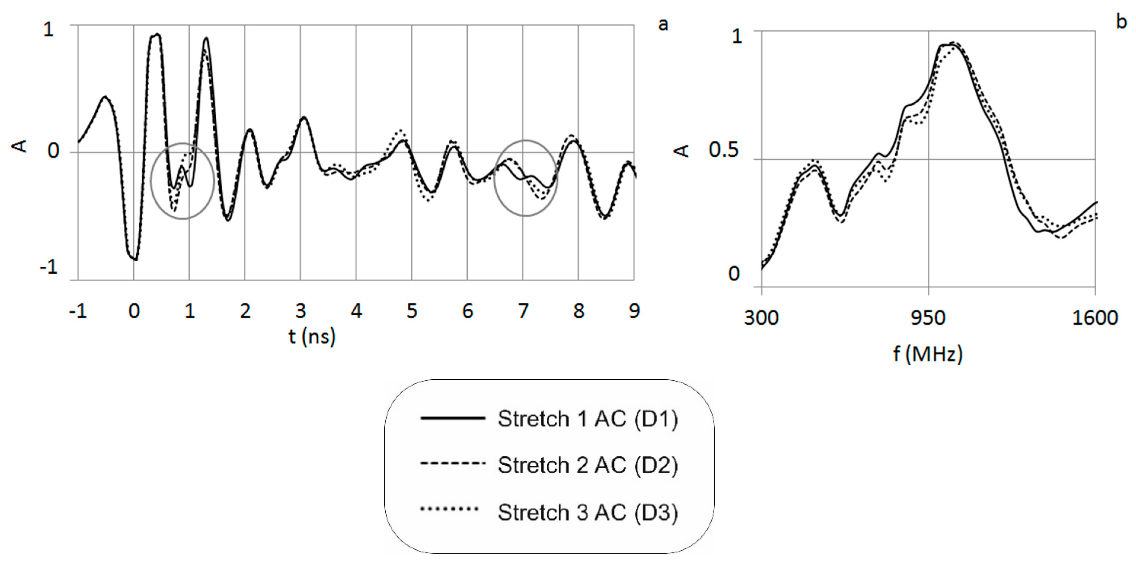
Figure 8, Figure 9, Figure 10 and Figure 11 show the results obtained for each sector according to their preservation condition. All of them show the wave trace diagrams (A-scans) in their time domain and the frequency spectra. These all correspond to the average of all the measurements carried out in a specific sector.
For each design cross-section, three stretches are considered that are represented in the following way: by a continuous line: the subsector in the best structural condition (D1); by a discontinuous line: the subsector in the intermediate condition (D2); finally, by a dotted line: the subsector that in the worst condition (D3). The results obtained from the type A pavement (Figure 2) are summarized in Figure 9.
In the left-hand diagram (Figure 9a), the A-scans of the three subsectors determined by their different degree of preservation are compared. It can be seen that the record pattern is the same in the three cases, except in the two specific areas that are marked with circles in Figure 9a. In these two areas, changes of amplitude occur corresponding to the signal reflections. These changes show discrepancies between the three averages. They are located around 0.8 ns and 7 ns, which correspond to the contact surfaces between wearing and binder courses, and base course and sub-grade. Assuming an average wave speed for a standard asphalt concrete of 10 cm/ns approximately, the signal reflections are located around 3 cm and 35 cm depth from the surface of pavement.
On analyzing the results for the same pavement typology with different preservation conditions (D1, D2, and D3), no relationship is observed between the double propagation time of the reflected wave and the structural condition of the pavement; therefore, it is deduced that the propagation time analysis does not provide relevant information with regard to the preservation condition of the pavement.
The diagram in Figure 9b shows the variation in the frequency spectrum for the three deterioration levels considered for the pavement. The maximum recorded for the highest frequencies associated with the combined bituminous mix layers remains virtually unchanged in the three spectra. However, in the case of the maximum peak associated with the sub-grades, located at about 900 MHz, corresponding to the second maximum, the higher amplitude is obtained for the signal obtained in the stretch in the best conditions (D1), and the maximum loses amplitude as the structure deteriorates.
These results suggest that the greatest deterioration of the structure would be found in the sub-grade, under the bituminous mix structure. A possible cause may be the debonding between layers or the breaking up of material in the sub-grade, which generates an energy dispersion effect and therefore a loss of energy.
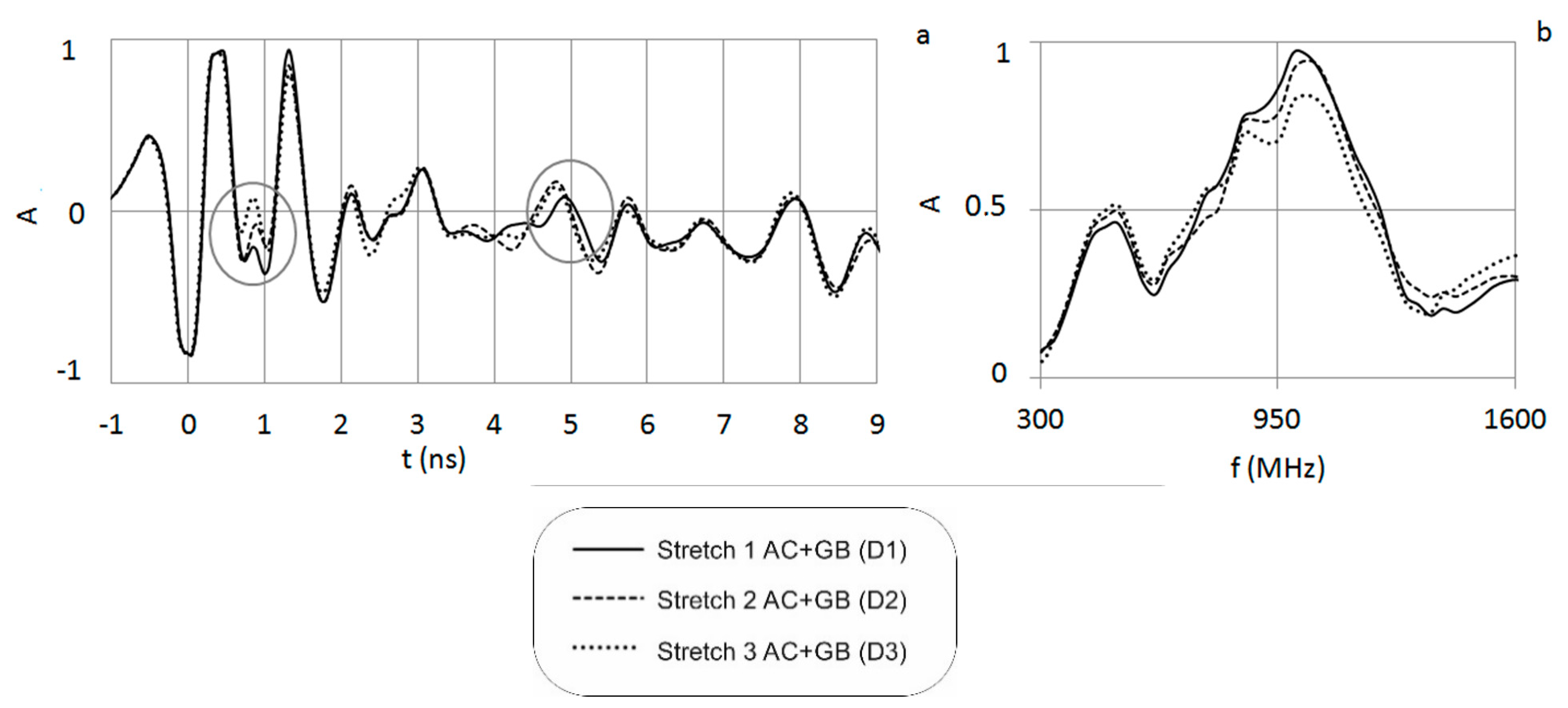
Figure 10 shows the results obtained in the studied subsector, characterized by a type B design cross-section.
In the diagram of Figure 10a, two amplitude changes can be seen in the trace again. They are located around 0.8 ns and 5 ns, which correspond to the interface between wearing and binder courses, and bituminous base course and granular base, respectively. Assuming an average wave speed for standard asphalt concrete, the signal reflections are located around 3 cm and 25 cm depth from the surface of pavement.
Stretches 2 and 3 show higher amplitude in the areas identified with circles. This phenomenon could be associated with a debonding process between layers [81].
The diagram in Figure 10b also shows the variation of the signal frequency spectrum in each one of the three subsectors.
In this case, the form of the spectrum and the location of its maximums, both that related to the combined bituminous mix layers and that related to the granular bases, change following the same pattern, i.e., the amplitude and bandwidth is maintained in the stretch in best condition, and they diminish as the structure deteriorates.
This result could indicate that in contrast to that occurring in the type A cross-section, the structural failure could take place in the system as a whole, i.e., in the AC and GB layers.
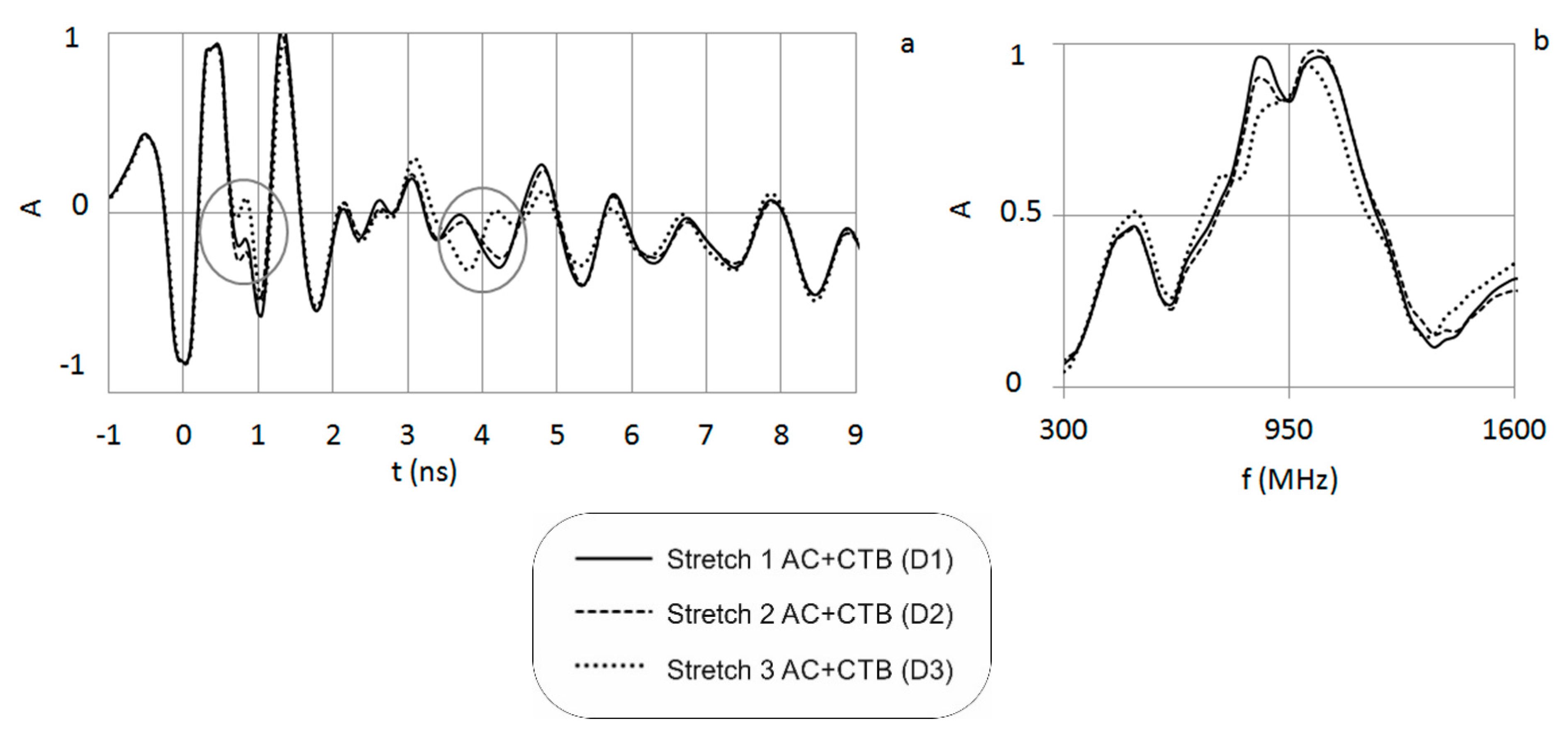
The graphs obtained in the study of the type C cross-section stretches are shown in Figure 11. In the diagram in Figure 11a, it can be seen that there are again two changes in the amplitude associated with the contacts between wearing course and binder course, and bituminous base course and cement-treated base. The second change is located around 4.2 ns for the best and intermediate stretch, and at 3.7 ns for the worst section (D3). An analysis similar to that carried out in the other tests gives a thickness of base course about 20 cm in the case of the best (D1) and intermediate (D2) subsectors, and 17 cm for the worst subsector. This thickness difference reveals the significant effect of the base course over the cement-treated base in the behavior of the structure (higher deflections).
In the diagram in Figure 11b, it can also be seen how the amplitude of the spectrum and the bandwidth decrease in the case of the graph that corresponds with the subsector in the worst conditions.
This data suggests that the failure in the structure could occur, among other reasons, due to the reduced thickness of the bituminous mix in this stretch of road.
Table 3 summarizes the main results, comparing in the three types of pavement, the three degrees of state of conservation (D1, D2, and D3).
4. Discussion and Conclusions
The GPR test is included in various pavement design guides in different countries. However, its use is usually restricted to propagation time analysis, there being few studies based on the frequency domain of the records.
The objective of the work was to analyse the frequency content of the spectrum of the signals recorded in various sectors of a stretch of road differentiated by their construction cross-sections. Each one of the sectors was subdivided into subsectors which were selected in a way that ensured their homogeneity, and within the criteria set out in the AASHTO pavement design guide. These subsectors were selected and classified in accordance with the results of the deflection and roughness tests carried out to find out their preservation condition.
It was the intention, therefore, to analyze the sensitivity of the frequency spectrum of the GPR records to changes in the construction typology and their state of preservation. The study is a first analysis to determine the capability of the proposed method; therefore, quantitative relationships are not determined between its sensitivity and the studied parameters. However, the results are promising and indicate the way in which these studies can be applied systematically.
The proposed methodology comprised a statistical analysis of a set of deflection values, IRI data and GPR records selected after deciding on some common criteria. Based on this selection, a results diagram was obtained in each case for evaluating the typology and the state of preservation of the studied pavement stretches. In the case of the GPR tests, diagrams averaged in the time and frequency domain are shown, and it was endeavored to ensure that they are sufficiently representative of each stretch. The results have led to the following conclusions:
- (1)
- The frequency spectrum is sensitive to the typology of material used in a pavement. Tests were carried out on stretches where different materials were used for the base: bituminous mixes, granular and cement-treated materials. In the comparative study, changes were observed in the amplitude maximums of the spectrum within the frequency range associated with that layer.
- (2)
- A statistical study of the wave transmitted to each medium allowed the amplitude changes recorded in the time domain to be determined, as a consequence of the reflections that occurred at the contacts or in the transition zones between the various layers that make up the pavement. This allowed the approximate average thicknesses of each one of the layers to be defined.
- (3)
- On obtaining the frequency spectrum of the time signals by means of the Fourier transform, their variations could be analyzed when the conditions of the media changed, which were studied from the time record. It can be seen that the frequency spectrum is sensitive to the structural condition of a pavement (this condition was previously defined based on a standardized deflection test). In all the analyzed cases, as the condition becomes worse, the amplitude of the frequency spectrum decreases as its bandwidth reduces. The tests carried out appear to indicate that the cause of these phenomena may be the debonding between layers or the breakup of the material in the sub-grade. This second problem would produce an increase in energy dispersion, thus attenuating the signal. The result would be a decrease in the energy recorded in the frequency range associated with the affected material and, therefore, a smaller amplitude in the area of the spectrum associated with that range.
- (4)
- Although none of the NDT technologies is capable of identifying partial or no bond due to inadequate tack coat during construction. GPR can identify variations in the pavement, isolate the depth of a discontinuity in the pavement, and provide a relative degree of severity. Severe conditions, such as stripping, can be observed with conventional analysis software. Detecting debonding between asphalt layers is only possible when there is moisture trapped in the debonded area between the layers using current analysis methodology, although the results indicates possible detection of those damages.
The results shows that GPR is sensitive to the different layers that make up an asphalt pavement. Furthermore, through the study of the response wave in its frequency domain it is possible to know whether the granular base is treated with cement or not. On the other hand, the amplitude generated by each frequency peak is also sensitive to its integrity condition. However, the tests have been carried out on a known structure with homogeneous thicknesses, which are also known. For this reason, it would be of great interest to be able to check whether the behavior of the response wave in its frequency domain is similar in pavements composed of an asphalt layer and a granular base or cement-treated base with different thicknesses. Should this be the case, the study could allow in the future to approximate a deflection value only by studying the shape of each peak generated by each pavement layer. Given that the GPR test is carried out at high speeds with a very high density of sampling (more data can be obtained per length unit with GPR than with deflection surveys), obtaining results in a very short time, it would be reasonable to use this method to define homogenous sections of a flexible pavement according to its characteristics, also approximating its maintenance condition.
Although the promising results showing the sensitivity of the spectrum to several characteristics and conditions of the pavement, further research is still needed to prove and confirm the conclusions and to consolidate the results. Future works might be focused on laboratory tests and numerical simulation of the spectrum behavior associate to changes in water content, debonding and number of layers. In addition, a statistical analysis based on field surveys could also be helpful to corroborate the results obtained in this work and to associate the different changes in the frequency content to particular features.
Author Contributions
Conceptualization, A.M.R., V.P.-G.; methodology, V.P.-G., J.P.R.; validation, A.M.R., V.P.-G.; formal analysis, A.M.R., V.P.-G.; investigation, J.P.R.; data acquisition, J.P.R., data processing, J.P.R.; data curation, J.P.R., A.M.R., V.P.-G.; writing—original draft preparation, J.P.R., A.M.R., V.P.-G.; writing—review and editing, A.M.R., V.P.-G.; supervision, A.M.R., V.P.-G. All authors have read and agreed to the published version of the manuscript.
Funding
This research has been partially funded by the Spanish Ministry of Economy and Competitiveness (MINECO) of the Spanish Government and by the European Regional Development Fund (FEDER) of the European Union (UE) through projects referenced as CGL2011-23621 and CGL2015-65913-P (MINECO/FEDER, UE). The study is also a contribution to the EU Action COST TU1208 “Civil Engineering Applications of Ground Penetrating Radar” financed by the European Union.
Acknowledgments
The authors would like to acknowledge the contribution of all those people and institutions that have helped and collaborated in the radar data acquisition tasks and in the various experimental tests.
Conflicts of Interest
The authors declare no conflict of interest.
References
- Stubstad, R.; Jiang, Y.; Lukanen, E. Forward calculation of pavement moduli with load-deflection data. Transp. Res. Rec. J. Transp. Res. Board 2007, 2005, 104–111. [Google Scholar] [CrossRef]
- Chea, S.; Martinez, J. Using Surface Deflection for Detection of Interface Damage between Pavement Layers. Road Mater. Pavement Des. 2008, 9, 359–372. [Google Scholar] [CrossRef]
- Lekarp, F.; Isacsson, U.; Dawson, A. State of the art. I: Resilient response of unbound aggregates. J. Transp. Eng. 2000, 126, 66–75. [Google Scholar] [CrossRef] [Green Version]
- Erlingsson, S. Impact of water on the response and performance of a pavement structure in an accelerated test. Road Mater. Pavement Des. 2010, 11, 863–880. [Google Scholar] [CrossRef]
- Cary, C.E.; Zapata, C.E. Resilient modulus for unsaturated unbound materials. Road Mater. Pavement Des. 2011, 12, 615–638. [Google Scholar] [CrossRef]
- Salour, F.; Erlingsson, S. Impact of Groundwater Level on the Mechanical Response of a Flexible Pavement Structure: A Case Study at the Torpsbruk Test Section along County road 126 Using Falling Weight Deflectometer; VTI: Linköping, Sweden, 2014. [Google Scholar]
- Gedafa, D.S.; Hossain, M.; Miller, R.; Van, T. Estimation of remaining service life of flexible pavements from surface deflections. J. Transp. Eng. 2009, 136, 342–352. [Google Scholar] [CrossRef] [Green Version]
- National Cooperative Highway Research Program. AASHTO Guide for Design of Pavement Structures; The American Association of State Highway and Transportation Officials: Washington, DC, USA, 1993. [Google Scholar]
- Crook, A.; Montgomery, S.; Guthrie, W. Use of Falling Weight Deflectometer Data for Network-Level Flexible Pavement Management. Transp. Res. Rec. J. Transp. Res. Board 2012, 2304, 75–85. [Google Scholar] [CrossRef]
- Horak, E. The use of surface deflection basin measurements in the mechanistic analysis of flexible pavements. In Sixth International Conference, Structural Design of Asphalt Pavements, Proceedings, University of Michigan, 13–17 July 1987; Michigan University: Ann Arbor, MI, USA, 1987; Volume I. [Google Scholar]
- Horak, E. Benchmarking the structural condition of flexible pavements with deflection bowl parameters. J. S. Afr. Inst. Civ. Eng. 2008, 50, 2–9. [Google Scholar]
- Donovan, P.; Tutumluer, E. Falling weight deflectometer testing to determine relative damage in asphalt pavement unbound aggregate layers. Transp. Res. Rec. J. Transp. Res. Board 2009, 2104, 12–23. [Google Scholar] [CrossRef] [Green Version]
- Park, K.; Thomas, N.E.; Wayne Lee, K. Applicability of the International Roughness Index as a Predictor of Asphalt Pavement Condition 1. J. Transp. Eng. 2007, 133, 706–709. [Google Scholar] [CrossRef]
- Arhin, S.A.; Williams, L.N.; Ribbiso, A.; Anderson, M.F. Predicting Pavement Condition Index using International Roughness Index in a Dense Urban Area. J. Civ. Eng. Res. 2015, 5, 10–17. [Google Scholar]
- Dewan, S.A.; Smith, R.E. Estimating IRI from pavement distresses to calculate vehicle operating costs for the cities and counties of San Francisco Bay area. Transp. Res. Rec. 2002, 1816, 65–72. [Google Scholar] [CrossRef]
- Capozzoli, L.; Rizzo, E. Combined NDT techniques in civil engineering applications: Laboratory and real test. Constr. Build. Mater. 2017, 154, 1139–1150. [Google Scholar] [CrossRef]
- Lagüela, S.; Solla, M.; Puente, I.; Prego, F.J. Joint use of GPR, IRT and TLS techniques for the integral damage detection in paving. Constr. Build. Mater. 2018, 174, 749–760. [Google Scholar] [CrossRef]
- Goel, A.; Das, A. Nondestructive testing of asphalt pavements for structural condition evaluation: A state of the art. Nondestruct. Test. Eval. 2008, 23, 121–140. [Google Scholar] [CrossRef]
- Marecos, V.; Fontul, S.; de Lurdes Antunes, M.; Solla, M. Evaluation of a highway pavement using non-destructive tests: Falling Weight Deflectometer and Ground Penetrating Radar. Constr. Build. Mater. 2017, 154, 1164–1172. [Google Scholar] [CrossRef]
- Borecky, V.; Haburaj, F.; Artagan, S.S.; Routil, L. Analysis of GPR and FWD data dependency based on road test field surveys. Mater. Eval. 2019, 77, 214–225. [Google Scholar]
- Plati, C.; Loizos, A.; Gkyrtis, K. Integration of non-destructive testing methods to assess asphalt pavement thickness. NDT E Int. 2020, 102292. [Google Scholar] [CrossRef]
- Pérez-Gracia, V.; Fontul, S.; Santos-Assunção, S.; Marecos, V. Geophysics: Fundamentals and Applications in Structures and Infrastructure. Non-Destr. Tech. Eval. Struct. Infrastruct. 2016, 11, 59. [Google Scholar]
- Solla, M.; Lorenzo, H.; Martínez-Sánchez, J.; Pérez-Gracia, V. Applications of GPR in association with other non-destructive testing methods in surveying of transport infrastructures. In Civil Engineering Applications of Ground Penetrating Radar; Springer: Cham, Switzerland, 2015; pp. 327–342. [Google Scholar]
- Moropoulou, A.; Avdelidis, N.P.; Koui, M.; Kakaras, K. An application of thermography for detection of delaminations in airport pavements. NDT E Int. 2001, 34, 329–335. [Google Scholar] [CrossRef]
- Solla, M.; Lagüela, S.; González-Jorge, H.; Arias, P. Approach to identify cracking in asphalt pavement using GPR and infrared thermographic methods: Preliminary findings. NDT E Int. 2014, 62, 55–65. [Google Scholar] [CrossRef]
- Plati, C.; Georgiou, P.; Loizos, A. Use of infrared thermography for assessing HMA paving and compaction. Transp. Res. Part C Emerg. Technol. 2014, 46, 192–208. [Google Scholar] [CrossRef]
- Hoegh, K.; Khazanovich, L.; Yu, H.T. Ultrasonic tomography for evaluation of concrete pavements. Transp. Res. Rec. 2011, 2232, 85–94. [Google Scholar] [CrossRef]
- Khazanovich, L.; Velasquez, R.; Nesvijski, E.G. Evaluation of top-down cracks in asphalt pavements by using a self-calibrating ultrasonic technique. Transp. Res. Rec. 2005, 1940, 63–68. [Google Scholar] [CrossRef]
- Behnia, B.; Buttlar, W.; Reis, H. Evaluation of low-temperature cracking performance of asphalt pavements using acoustic emission: A review. Appl. Sci. 2018, 8, 306. [Google Scholar] [CrossRef] [Green Version]
- Apeagyei, A.K.; Buttlar, W.G.; Reis, H. Assessment of low-temperature embrittlement of asphalt binders using an acoustic emission approach. Insight-Non-Destr. Test. Cond. Monit. 2009, 51, 129–136. [Google Scholar] [CrossRef] [Green Version]
- Al-Qadi, I.L.; Lahouar, S. Measuring layer thicknesses with GPR–Theory to practice. Constr. Build. Mater. 2005, 19, 763–772. [Google Scholar] [CrossRef]
- Lahouar, S.; Al-Qadi, I.L. Automatic detection of multiple pavement layers from GPR data. NDT E Int. 2008, 41, 69–81. [Google Scholar] [CrossRef]
- Le Bastard, C.; Baltazart, V.; Wang, Y.; Saillard, J. Thin-pavement thickness estimation using GPR with high-resolution and superresolution methods. IEEE Trans. Geosci. Remote Sens. 2007, 45, 2511–2519. [Google Scholar] [CrossRef]
- Diamanti, N.; Redman, D. Field observations and numerical models of GPR response from vertical pavement cracks. J. Appl. Geophys. 2012, 81, 106–116. [Google Scholar] [CrossRef]
- Krysiński, L.; Sudyka, J. GPR abilities in investigation of the pavement transversal cracks. J. Appl. Geophys. 2013, 97, 27–36. [Google Scholar] [CrossRef]
- Rasol, M.A.; Pérez-Gracia, V.; Solla, M.; Pais, J.C.; Fernandes, F.M.; Santos, C. An experimental and numerical approach to combine Ground Penetrating Radar and computational modelling for the identification of early cracking in cement concrete pavements. NDT E Int. 2020, 102293. [Google Scholar] [CrossRef]
- Rasol, M.A.; Pérez-Gracia, V.; Fernandes, F.M.; Pais, J.C.; Santos-Assunçao, S.; Santos, C.; Sossa, V. GPR laboratory tests and numerical models to characterize cracks in cement concrete specimens, exemplifying damage in rigid pavement. Measurement 2020, 158, 107662. [Google Scholar] [CrossRef]
- Liu, H.; Sato, M. In situ measurement of pavement thickness and dielectric permittivity by GPR using an antenna array. NDT E Int. 2014, 64, 65–71. [Google Scholar] [CrossRef]
- Grote, K.; Hubbard, S.; Harvey, J.; Rubin, Y. Evaluation of infiltration in layered pavements using surface GPR reflection techniques. J. Appl. Geophys. 2005, 57, 129–153. [Google Scholar] [CrossRef]
- Plati, C.; Loizos, A. Estimation of in-situ density and moisture content in HMA pavements based on GPR trace reflection amplitude using different frequencies. J. Appl. Geophys. 2013, 97, 3–10. [Google Scholar] [CrossRef]
- Heitzman, M.; Maser, K.; Tran, N.H.; Brown, R.; Bell, H.; Holland, S.; Hiltunen, D. Nondestructive Testing to Identify Delaminations between HMA Layers; Transportation Research Board: Washington, DC, USA, 2013. [Google Scholar]
- Pedret Rodes, J.; Pérez-Gracia, V.; Martínez-Reguero, A. Evaluation of the GPR frequency spectra in asphalt pavement assessment. Constr. Build. Mater. 2015, 96, 181–188. [Google Scholar] [CrossRef] [Green Version]
- Salvi, R.; Ramdasi, A.; Kolekar, Y.A.; Bhandarkar, L.V. Use of Ground-Penetrating Radar (GPR) as an Effective Tool in Assessing Pavements—A Review. In Geotechnics for Transportation Infrastructure; Springer: Singapore, 2019; pp. 85–95. [Google Scholar]
- Plati, C.; Loizos, A.; Gkyrtis, K. Assessment of Modern Roadways Using Non-destructive Geophysical Surveying Techniques. Surv. Geophys. 2020, 41, 295–430. [Google Scholar] [CrossRef]
- Evans, R.D.; Frost, M.; Stonecliffe-Jones, M.; Dixon, N. A Review of Pavement Assessment Using Ground Penetrating Radar (GPR) in 12th International Conference on Ground Penetrating Radar, 16–19 June 2008; Universty of Birmingham and EuroGPR: Birmingham, UK, 2008. [Google Scholar]
- Saarenketo, T.; Scullion, T. Road evaluation with ground penetrating radar. J. Appl. Geophys. 2000, 43, 119–138. [Google Scholar] [CrossRef]
- Daniels, D.J. Ground Penetrating Radar, Ser. IEE Radar, Sonar, Navigation and Avionics Series; The Institution of Electrical Engineers: London, UK, 2004. [Google Scholar]
- Al-Qadi, I.L.; Lahouar, S.; Loulizi, A. In situ measurements of hot-mix asphalt dielectric properties. NDT E Int. 2001, 34, 427–434. [Google Scholar] [CrossRef]
- Evans, R.; Frost, M.; Stonecliffe-Jones, M.; Dixon, N. Assessment of in situ dielectric constant of pavement materials. Transp. Res. Rec. 2007, 2037, 128–135. [Google Scholar] [CrossRef] [Green Version]
- ASTM. D4748-06 Standard Test Method for Determining the Thickness of Bound Pavement Layers Using Short-Pulse Radar; American Society for Testing and Materials: West Conshohocken, PA, USA, 2006. [Google Scholar]
- Loizos, A.; Plati, C. Accuracy of pavement thicknesses estimation using different ground penetrating radar analysis approaches. NDT E Int. 2007, 40, 147–157. [Google Scholar] [CrossRef]
- Varela-González, M.; Solla, M.; Martínez-Sánchez, J.; Arias, P. A semi-automatic processing and visualisation tool for ground-penetrating radar pavement thickness data. Autom. Constr. 2014, 45, 42–49. [Google Scholar] [CrossRef]
- Marecos, V.; Fontul, S.; Solla, M.; de Lurdes Antunes, M. Evaluation of the feasibility of Common Mid-Point approach for air-coupled GPR applied to road pavement assessment. Measurement 2018, 128, 295–305. [Google Scholar] [CrossRef]
- Wang, S.; Zhao, S.; Al-Qadi, I.L. Continuous real-time monitoring of flexible pavement layer density and thickness using ground penetrating radar. NDT E Int. 2018, 100, 48–54. [Google Scholar] [CrossRef]
- Fernandes, F.M.; Pais, J.C. Laboratory observation of cracks in road pavements with GPR. Constr. Build. Mater. 2017, 154, 1130–1138. [Google Scholar] [CrossRef]
- Saarenketo, T. Recommendations for Guidelines for the Use of GPR in Asphalt Air Voids Content Measurement. Interreg IVA Nord Program, Mara Nord Proyect; Päällystetutkaajat Oy: Rovaniemi, Finland, 2012; pp. 5–22. [Google Scholar]
- Shang, J.Q.; Umana, J.A.; Bartlett, F.M.; Rossiter, J.R. Measurement of complex permittivity of asphalt pavement materials. J. Transp. Eng. 1999, 125, 347–356. [Google Scholar] [CrossRef]
- Jaselskis, E.J.; Grigas, J.; Brilingas, A. Dielectric properties of asphalt pavement. J. Mater. Civ. Eng. 2003, 15, 427–434. [Google Scholar] [CrossRef]
- Zhang, J.; Yang, X.; Li, W.; Zhang, S.; Jia, Y. Automatic detection of moisture damages in asphalt pavements from GPR data with deep CNN and IRS method. Autom. Constr. 2020, 113, 103119. [Google Scholar] [CrossRef]
- Zhang, J.; Zhang, C.; Lu, Y.; Zheng, T.; Dong, Z.; Tian, Y.; Jia, Y. In-situ recognition of moisture damage in bridge deck asphalt pavement with time-frequency features of GPR signal. Constr. Build. Mater. 2020, 244, 118295. [Google Scholar] [CrossRef]
- Benedetto, A. Water content evaluation in unsaturated soil using GPR signal analysis in the frequency domain. J. Appl. Geophys. 2010, 71, 26–35. [Google Scholar] [CrossRef]
- Lai, W.L.; Kind, T.; Wiggenhauser, H. A study of concrete hydration and dielectric relaxation mechanism using ground penetrating radar and short-time Fourier transform. EURASIP J. Adv. Signal Process. 2010, 2010, 12. [Google Scholar] [CrossRef] [Green Version]
- Dérobert, X.; Villain, G.; Cortas, R.; Chazelas, J.L. EM characterization of hydraulic concretes in the GPR frequency band using a quadratic experimental design. Presented at the NDT Conference on Civil Engineering, Nantes, France, 30 June–3 July 2009; pp. 177–182. [Google Scholar]
- Bano, M. Modelling of GPR waves for lossy media obeying a complex power law of frequency for dielectric permittivity. Geophys. Prospect. 2004, 52, 11–26. [Google Scholar] [CrossRef] [Green Version]
- Pérez-Gracia, V.; González-Drigo, R.; Di Capua, D. Horizontal resolution in a non-destructive shallow GPR survey: An experimental evaluation. NDT E Int. 2008, 41, 611–620. [Google Scholar] [CrossRef]
- Laurens, S.; Balayssac, J.P.; Rhazi, J.; Klysz, G.; Arliguie, G. Non-destructive evaluation of concrete moisture by GPR: Experimental study and direct modeling. Mater. Struct. 2005, 38, 827–832. [Google Scholar] [CrossRef]
- Santos-Assunçao, S.; Krishna, S.; Perez-Gracia, V. GPR analysis of water content in concrete specimen-laboratory test. In Near Surface Geoscience 2016-22nd European Meeting of Environmental and Engineering Geophysics; European Association of Geoscientists & Engineers: Houten, The Netherlands, 2016; Volume 2016, p. cp-495. [Google Scholar]
- Sbartaï, Z.M.; Laurens, S.; Breysse, D. Concrete moisture assessment using radar NDT technique: Comparison between time and frequency domain analysis. Presented at the Non-Destructive Testing in Civil Engineering (NDTCE ’09), Nantes, France, 30 June–3 July 2009. [Google Scholar]
- Santos-Assunçao, S.; Perez-Gracia, V.; González-Drigo, R.; Salinas, V.; Caselles, O. Ground Penetrating Radar Applications in Seismic Microzonation. In Near Surface Geoscience 2015-21st European Meeting of Environmental and Engineering Geophysics; European Association of Geoscientists & Engineers: Houten, The Netherlands, 2015; Volume 2015, pp. 1–5. [Google Scholar]
- Cui, F.; Wu, Z.Y.; Wang, L.; Wu, Y.B. Application of the Ground Penetrating Radar ARMA power spectrum estimation method to detect moisture content and compactness values in sandy loam. J. Appl. Geophys. 2015, 120, 26–35. [Google Scholar] [CrossRef]
- Tosti, F.; Patriarca, C.; Slob, E.; Benedetto, A.; Lambot, S. Clay content evaluation in soils through GPR signal processing. J. Appl. Geophys. 2013, 97, 69–80. [Google Scholar] [CrossRef]
- Benedetto, F.; Tosti, F. GPR spectral analysis for clay content evaluation by the frequency shift method. J. Appl. Geophys. 2013, 97, 89–96. [Google Scholar] [CrossRef]
- Benedetto, A.; Tosti, F.; Ortuani, B.; Giudici, M.; Mele, M. Mapping the spatial variation of soil moisture at the large scale using GPR for pavement applications. Near Surf. Geophys. 2015, 13, 269–278. [Google Scholar] [CrossRef]
- Tosti, F.; Benedetto, A.; Ciampoli, L.B.; Lambot, S.; Patriarca, C.; Slob, E.C. GPR analysis of clayey soil behaviour in unsaturated conditions for pavement engineering and geoscience applications. Near Surf. Geophys. 2016, 14, 127–144. [Google Scholar] [CrossRef]
- Dirección General de Carreteras del Ministerio de Fomento. Orden Circular 10/2002 Sobre Secciones de Firme y Capas Estructurales de Firmes; Dirección General de Carreteras del Ministerio de Fomento: Madrid, Spain, 2002. [Google Scholar]
- AASHTO. American Association of State Highway and Transportation Officials Guide for Design of Pavement Structures; AASHTO: Washington, DC, USA, 1986. [Google Scholar]
- Prandi, E. The Lacroix-LCPC Deflectograph. In Intl Conf Struct Design Asphalt Pvmts; The National Academies of Sciences, Engineering, and Medicine: Washington, DC, USA, 1967. [Google Scholar]
- Santos.Assunçao, S. Ground Penetrating Radar Applications in Seismic Zonation: Assessment and Evaluation. Ph.D. Thesis, Universitat Politècnica de Catalunya (UPC), Barcelona, Spain, 2014. [Google Scholar]
- Solla, M.; González-Jorge, H.; Lorenzo, H.; Arias, P. Uncertainty evaluation of the 1 GHz GPR antenna for the estimation of concrete asphalt thickness. Measurement 2013, 46, 3032–3040. [Google Scholar] [CrossRef]
- Lorenzo Cimadevilla, H. Prospección Geofísica de Alta Resolución Mediante Geo-Radar; Aplicación a Obras Civiles; Laboratorio de Geotecnia del CEDEX: Madrid, Spain, 1996; p. 196. [Google Scholar]
- Sudyka, J.; Krysiński, L. Radar Technique Application in Structural Analysis and Identification of Interlayer Bonding. Int. J. Pavement Res. Technol. 2011, 4, 176–184. [Google Scholar]
Figure 1.
Scheme of GPR assessment of pavements. The antennas are usually mounted in a platform in a car. The existence of changes in the electromagnetic parameters produce the reflection of the energy that is detected by the receiver antenna. The result is the B-scan that includes the amplitude of the signals and the two-way travel time, in front of the position of each individual A-scan.

Figure 2.
Design cross-sections, type A full depth asphalt (a), B flexible (b) and C semi-rigid pavement with treated cement base (c).
Figure 2.
Design cross-sections, type A full depth asphalt (a), B flexible (b) and C semi-rigid pavement with treated cement base (c).

Figure 3.
Deflection test cumulative frequency histograms in cross-section type A (a), type B (b) and type C (c).
Figure 3.
Deflection test cumulative frequency histograms in cross-section type A (a), type B (b) and type C (c).

Figure 4.
Roughness test cumulative frequency histograms (IRI) in cross-section type A (a), type B (b) and type C (c).
Figure 4.
Roughness test cumulative frequency histograms (IRI) in cross-section type A (a), type B (b) and type C (c).

Figure 5.
Radar data acquisition with a 900 MHz center frequency antenna.

Figure 6.
Characteristics of the antenna used. Recorded wave (a) and frequency spectrum (b).

Figure 7.
Results obtained in a cross-section without defects. (a) Core showing the structural layers. (b) A-scan, in the time domain. (c) Frequency content of the signal considering three time windows that are defined considering the core layers and the A-scan. (d) Frequency spectrum of the A-scan 1. The contribution determined in the three time windows define the peaks observed in the spectrum.

Figure 8.
Frequency spectra of the construction cross-sections. Averaged results for each subsector (a) and standard deviation of the averaged spectra (b).
Figure 8.
Frequency spectra of the construction cross-sections. Averaged results for each subsector (a) and standard deviation of the averaged spectra (b).

Figure 9.
Time domain (a) and frequency spectra (b) in the three subsectors of the type A cross-section.
Figure 9.
Time domain (a) and frequency spectra (b) in the three subsectors of the type A cross-section.

Figure 10.
Time domain (a) and frequency spectra (b) in the three subsectors of the type B cross-section.
Figure 10.
Time domain (a) and frequency spectra (b) in the three subsectors of the type B cross-section.

Figure 11.
Time domain (a) and frequency spectra (b) in the three subsectors of the type C cross-section.
Figure 11.
Time domain (a) and frequency spectra (b) in the three subsectors of the type C cross-section.


Table 1.
Stretches studied with the deflection and surface roughness (IRI) test results. Being: AC, Asphalt concrete; GB, Granular Base; and CTB, Cement-treated Base. D1, D2 and D3 are the classification of zones; the increasing numbers indicate increasing deflection ranges.
Table 1.
Stretches studied with the deflection and surface roughness (IRI) test results. Being: AC, Asphalt concrete; GB, Granular Base; and CTB, Cement-treated Base. D1, D2 and D3 are the classification of zones; the increasing numbers indicate increasing deflection ranges.
| Section | Design Section | Condition | Initial K.P. (km) | Final K.P. (km) | Tested Length (m) | Deflection (μm) | IRI (m/km) |
|---|---|---|---|---|---|---|---|
| A | AC (35 cm) | D1 | 60 + 400 | 61 + 100 | 700 | 82 | 0.9 |
| D2 | 61 + 100 | 61 + 800 | 700 | 94 | 1 | ||
| D3 | 61 + 800 | 62 + 500 | 700 | 103 | 1 | ||
| B | AC (25 cm) + GB (25 cm) | D1 | 71 + 600 | 72 + 600 | 1000 | 53 | 0.9 |
| D2 | 66 + 000 | 67 + 000 | 1000 | 90 | 0.9 | ||
| D3 | 68 + 200 | 69 + 200 | 1000 | 130 | 1.7 | ||
| C | AC (20 cm) + CTB (25 cm) | D1 | 77 + 000 | 78 + 000 | 1000 | 26 | 0.7 |
| D2 | 78 + 000 | 79 + 000 | 1000 | 24 | 1 | ||
| D3 | 80 + 300 | 81 + 300 | 700 | 82 | 1.3 |
Table 2.
Characteristics of layers AC, GB and CTB [80].
Table 2.
Characteristics of layers AC, GB and CTB [80].
| Layer Type | Relative Dielectric Permittivity (εr) | Electrical Resistivity (σ) (Ωm) |
|---|---|---|
| AC | 7.6–8.2 | 0.001 |
| GB | 4.5–4.8 | 0.001 |
| CTB | 15.9 | 0.1 |
Table 3.
Main results, highlighting the changes in the spectra as consequence of the deflection ranges D1, D2 and D3, for each one of the three types of pavement.
Table 3.
Main results, highlighting the changes in the spectra as consequence of the deflection ranges D1, D2 and D3, for each one of the three types of pavement.
| Stretch | Spectrum | A-Scan | Possible Damage in Case D3 | |
|---|---|---|---|---|
| Peak 1 (900 MHz) | Peak 2 (1100 MHz) | |||
| AC | Maximum amplitude in D1 and minimum amplitude in D2 | Same amplitude approximately in D1, D2 and D3 | Small changes of amplitude in contacts when comparing D1, D2 and D3 | Possible damage under bituminous layer (AC): possible debonding or damage in sub-grade |
| AC + GB | Amplitude diminish as structure deteriorates (maximum amplitude in D1 and minimum in D3) | Amplitude diminish as structure deteriorates (maximum amplitude in D1 and minimum in D3), with an important decrease in the case D3 | Clear changes of amplitude, being higher the amplitude in the contacts in the case of worst pavement conditions (D3) | Damage in both AC and Gb layers. Possible debonding |
| AC + CTB | Amplitude diminish as structure deteriorates (maximum amplitude in D1 and minimum in D3) | No evident changes of amplitude | Change of amplitude and phase in the second contact | Possible damage in the bituminous layer AC and in layer CTB |
© 2020 by the authors. Licensee MDPI, Basel, Switzerland. This article is an open access article distributed under the terms and conditions of the Creative Commons Attribution (CC BY) license (http://creativecommons.org/licenses/by/4.0/).
Share and Cite
MDPI and ACS Style
Pedret Rodés, J.; Martínez Reguero, A.; Pérez-Gracia, V. GPR Spectra for Monitoring Asphalt Pavements. Remote Sens. 2020, 12, 1749. https://doi.org/10.3390/rs12111749
AMA Style
Pedret Rodés J, Martínez Reguero A, Pérez-Gracia V. GPR Spectra for Monitoring Asphalt Pavements. Remote Sensing. 2020; 12(11):1749. https://doi.org/10.3390/rs12111749
Chicago/Turabian StylePedret Rodés, Josep, Adriana Martínez Reguero, and Vega Pérez-Gracia. 2020. "GPR Spectra for Monitoring Asphalt Pavements" Remote Sensing 12, no. 11: 1749. https://doi.org/10.3390/rs12111749
Note that from the first issue of 2016, this journal uses article numbers instead of page numbers. See further details here.