Volume Variations of Small Inland Water Bodies from a Combination of Satellite Altimetry and Optical Imagery


Deutsches Geodätisches Forschungsinsitut der Technischen Universität München (DGFI-TUM), Arcisstraße 21, 80333 München, Germany
*
Author to whom correspondence should be addressed.
Remote Sens. 2020, 12(10), 1606; https://doi.org/10.3390/rs12101606
Submission received: 2 April 2020
/
Revised: 11 May 2020
/
Accepted: 12 May 2020
/
Published: 18 May 2020
(This article belongs to the Special Issue Remote Sensing in Hydrology and Water Resources Management)
Abstract
:In this study, a new approach for estimating volume variations of lakes and reservoirs using water levels from satellite altimetry and surface areas from optical imagery is presented. Both input data sets, namely water level time series and surface area time series, are provided by the Database of Hydrological Time Series of Inland Waters (DAHITI), developed and maintained by the Deutsches Geodätisches Forschungsinsitut der Technischen Universität München (DGFI-TUM). The approach is divided into three parts. In the first part, a hypsometry model based on the new modified Strahler approach is computed by combining water levels and surface areas. The hypsometry model describes the dependency between water levels and surface areas of lakes and reservoirs. In the second part, a bathymetry between minimum and maximum surface area is computed. For this purpose, DAHITI land-water masks are stacked using water levels derived from the hypsometry model. Finally, water levels and surface areas are intersected with the bathymetry to estimate a time series of volume variations in relation to the minimum observed surface area. The results are validated with volume time series derived from in-situ water levels in combination with bathymetric surveys. In this study, 28 lakes and reservoirs located in Texas are investigated. The absolute volumes of the investigated lakes and reservoirs vary between 0.062 km and 6.041 km. The correlation coefficients of the resulting volume variation time series with validation data vary between 0.80 and 0.99. Overall, the relative errors with respect to volume variations vary between 2.8% and 14.9% with an average of 8.3% for all 28 investigated lakes and reservoirs. When comparing the resulting RMSE with absolute volumes, the absolute errors vary between 1.5% and 6.4% with an average of 3.1%. This study shows that volume variations can be calculated with a high accuracy which depends essentially on the quality of the used water levels and surface areas. In addition, this study provides a hypsometry model, high-resolution bathymetry and water level time series derived from surface areas based on the hypsometry model. All data sets are publicly available on the Database of Hydrological Time Series of Inland Waters.

1. Introduction
In the last years, discussions about global climate change have been increasing in the media and society, especially in connection with originators of climate change. Numerous climate studies are based on remote sensing data [1,2]. Since the 1970s, remote sensing has been providing valuable data for monitoring the global water cycle and its changes. Compared to the global water storage, only 0.013% [3] of the Earth‘s water is stored in lakes and reservoirs which are often affected by the impact of climate change. Since the 1980s, the number of reported flood events of inland waters has increased by 38% from about 150 to more than 400 in 2008 [4]. Human influences on the terrestrial water such as the construction of dams or agricultural irrigation has also increased in last decades. In the worst case, the resulting water scarcity can lead to political crisis or wars [5]. Therefore, the impact of climate change on the availability of fresh water for human consumption is immense. In future, this will require sustainable water management by the countries [6]. Independent monitoring of inland waters is therefore essential. However, since the 1980s, the number of publicly accessible in-situ measurements has been steadily decreasing which is reflected in the data holding of the Global Runoff Data Center [7]. Especially in remote areas and in developing countries, there is a lack of in-situ measurements. Today, existing data gaps can be often filled by using remote sensing technology which has already provided valuable information about changes on Earth.
Modeling and understanding of the terrestrial water cycle is of great importance for analyses of climate change [8]. Hydrological models have been developed to gain more knowledge. Hydrological models such as the WaterGAP Global Hydrology Model (WHGM) use storage changes of lakes and reservoirs and river discharge to quantify the amount of water on Earth [9]. Data from the Gravity Recovery and Climate Experiment (GRACE), which measures the total water storage, are often used for calibration and data assimilation of hydrological models [10]. However, due to the spatial resolution of about 300 km and the required separation of the signal into surface water, soil moisture, and groundwater [11], GRACE cannot be used to derive volume changes of water bodies directly. GRACE has already been used in several studies to correct leakage errors [12] or to compare them with other geometrical approaches [13,14] to estimate volume changes of lakes.
Satellite altimetry was originally designed to monitor the sea surface and the existing sea level rise since the 1990s. For more than two decades, satellite altimetry has also proven its worth for monitoring water level changes of lakes, reservoirs and rivers [15,16,17,18,19]. Since satellite altimetry measures in nadir direction, only the water body directly crossed by a satellite track can be investigated. To reach water levels with an accuracy between several centimetres and several decimetres, the crossing track requires a track length above water of about a few hundred meters.
Since the 1970s, optical imagery has been used to monitor changes on the Earth’s surface, such as flooded regions [20] or wetlands [21]. The Landsat mission with the satellites of Landsat-4/-5/-7/-8 has been providing optical images with constant quality since 1982. The Sentinel-2 mission has been providing high-resolution optical images for monitoring inland waters since 2015. In [22] an automated approach was shown that combines both data sets to extract surface areas of lakes and reservoirs.
The estimation of volume changes requires the most accurate bathymetry and water levels. The generation of both data sets can be done with different approaches which have already been used in different studies. The most precise approach for estimating volume changes is to use ground measurements. For this purpose, water levels from in-situ stations are combined with bathymetry based on ship surveys. This approach is carried out by the Texas Water Development Board (TWDB, https://www.waterdatafortexas.org) for about 120 lakes and reservoirs in Texas. The disadvantages of this method are that the surveys are time-consuming, cost a lot of money and are not easily applicable in remote areas. However, these data sets are very accurate and can therefore be used to validate volume changes based on remote sensing approaches. Up to now, it is not possible to measure the bathymetry of deeper lakes and reservoirs with the help of optical remote sensing images, because the light is attenuated as it enters the water. Even if several studies have successfully shown the potential for estimating bathymetry in shallow waters such as in coastal zones or shallow lakes [23,24,25], this technique can currently not be used for operational lake volume computation. Other studies estimated the lake bathymetry using the surrounding topographic slopes derived from a digital elevation model (DEM) [26]. Classical approaches for estimating volume changes of lakes and reservoirs are based on the combination of water levels from satellite altimetry and surface areas from optical images. However, the data sources used and the coupling methods applied to estimate volume changes differ considerably, which is shown in the following. Here, water levels from satellite altimetry (Global Reservoir and Lake Monitor, Hydroweb, ICESat, River Lake Hydrology) are combined with surface areas derived from a few selected Landsat images by applying a polynomial function of degree 2 for the estimation of the hypsometric curve [27]. This approach was applied to three lakes with volumes between 5.5 km and 35.5 km and yielded percentage errors between 4.62% and 13.08%. In another study, water levels from satellite altimetry (Global Reservoir and Lake Monitor, Hydroweb, River Lake Hydrology) and surface areas derived from MODIS are combined with a linear hypsometry model [28]. The approach is applied on 34 globally distributed reservoirs with a volume between 3 km and 165 km. Another approach is to use water levels obtained from IceSAT and corresponding surface images from Landsat and MODIS of Lake Poopó. The resulting contour lines are then interpolated to obtain a partial bathymetry [29]. In another study, the satellite altimetry of Hydroweb is combined with selected images from Landsat and MODIS to estimate a hypsometric model [30]. This involves adjusting polynomial functions of degree 1, 2 or 3, depending on the relationship. Finally, the time series of the volume variations are calculated using a pyramidal approach. This approach showed 24 lakes and reservoirs with a surface area between 350 km and 82,200 km. In a further study, 137 lakes and reservoirs are analyzed by combining water levels from DAHITI and monthly land water masks from the JRC Global Surface Water (GSW) data set based on Landsat data. The volumes are calculated for lakes that have a linear relationship between water level and surface areas. Therefore, volume changes are estimated for consecutive changes of water level and surface area [31].
In this paper, a new approach to calculate time series of volume variations of small lakes and reservoirs (≤6.0 km, ≤782 km) is presented. For this purpose, water levels from satellite altimetry and high-resolution surface areas from optical imagery are combined to estimate a hypsometry model. Then, the hypsometry model is used to reconstruct water levels from surface areas to compute a bathymetry above the smallest available surface area. Afterwards, water levels and surface areas are intersected with the bathymetry to calculate a time series of volume variation with respect to the smallest surface area. Finally, all resulting time series of volume variation of 28 selected water bodies are validated with in-situ storage changes. In contrast to existing similar approaches, the quality and number of data sets used in this study differ. Since we are using more data of higher precision, as well as an advanced combination approach, our approach yield better accuracies also for smaller water bodies.
This paper is organized as follows. In Section 2, all the investigated 28 water bodies are introduced. Section 3 describes the data used for processing and validation. Section 4 describes in detail the methodology for combining water levels from satellite altimetry and surface areas from optical images to estimate volume changes. In Section 5, the new approach for estimating volume variations is presented in detail for three selected water bodies, followed by a validation and quality assessment of all water bodies. Finally, a summary and discussion of the results as well as an outlook is given.
2. Water Bodies
For the demonstration and validation of the new approach, we have selected 28 lakes and reservoirs in Texas, USA, which are shown in Figure 1. All selected study areas are well monitored by the Texas Water Development Board (TWDB). The TWDB provides in-situ water levels, ship survey data, bathymetry data, hypsometric curves, height-area-volume relationships, and detailed reports for each selected water body. This information is essential for a reliable quality assessment of our results.
Table 1 gives an overview of the 28 water bodies and their characteristics. For each water body, the minimum, maximum and variation of water level, surface area and volume are given based on in-situ data.
3. Data
In this study, water levels from satellite altimetry and surface areas from optical imagery are used to calculate time series of volume variations for lakes and reservoirs. For validation and quality assessment, we use water levels from in-situ stations, surface areas derived from bathymetric surveys and volumes resulting from the combination of water levels and bathymetry. Figure 2 gives a detailed overview of the data availability of the input data and validation data used for each of the 28 water bodies.
3.1. In Situ Data
The availability of in-situ data is essential to assess the quality of our results. We deal with three different types of data sets, but only for one of them, ground truth data is available. Firstly, water levels from satellite altimetry are used which can be easily validated by using in-situ stations. However, surface areas and volume variations cannot be validated in a suitable way without an accurate bathymetry of the investigated lakes or reservoirs. Usually, bathymetry data are obtained by ship surveys measuring the lake bottom. In combination with in-situ water levels, surface areas and absolute volumes can be derived in a good quality for validation.
The Texas Water Development Board (TWDB, http://www.twdb.texas.gov/) provides water levels, surface areas and volumes for approximately 120 lakes and reservoirs in Texas which will be used to validate this study. The water levels are derived from in-situ stations maintained primarily in cooperation with the United States Geological Survey (USGS). In addition, the TWDB carries out bathymetry surveys which are conducted at irregular intervals. The lake volumes are then calculated using rating curves. However, since the bathymetry surveys refer to the water level on the day of the survey, no directly measured surface areas and volumes are available above that level. These values can only be estimated by extrapolating the calculated rating curve. This fact must be taken into account when validating the resulting volume variations in this study. The surface area time series and volume time series provided in the TWDB can also contain offsets between time periods of the recalculated rating curves. Remaining offsets are corrected to obtain consistent time series for validation. In addition, the TWDB provides reports for each water body containing detailed information on the surveys and the calculated height-area-volume relationships. This is very helpful in this study to understand and analyse inconsistencies in the time series used for validation.
We use the TWDB data holding to validate our results. Water level time series and surface areas time series are used for the quality assessment of the inputs used. In addition, we use the absolute volume time series to validate the resulting time series of volume variations. This is done for 28 investigated lakes and reservoirs in Texas. Figure 2 shows the data availability of water levels (light blue), surface areas (orange) and volumes (light green) provided by USGS/TWDB and used for validation in this study.
3.2. Water Level Time Series from Satellite Altimetry
In 1992, Topex/Poseidon was launched as the first operational satellite for monitoring sea level. Since then, several altimeter missions have been launched with improved equipment. In the last few decades, satellite altimetry has also been used for hydrological application such as measuring water levels of lakes, reservoirs, rivers and wetlands. Envisat was the first altimeter mission with the potential to derive water level time series of smaller lakes and rivers with sufficient accuracy between a few centimeters and a few decimeters. However, not all inland waters can be investigated, as the altimeter satellites only measure in nadir direction.
DGFI-TUM developed an approach to derive water level time series for lakes, reservoirs, rivers and wetlands. This method is based on a Kalman filtering approach and extended outlier detection [18]. In the first step, all measurements of different altimeter missions are homogenized by using identical geophysical corrections and models. Additionally, a multi-mission cross-calibration is applied to minimize range biases between different altimeter missions [32]. Then, outliers are rejected for each crossing altimeter track by applying different thresholds (e.g., latitude, water level, height error, etc.). Finally, the remaining water levels and their errors are combined in a sequential least square approach to achieve one water level for each day.
Currently, DGFI-TUM‘s web portal DAHITI makes more than 2600 respective water level time series freely available. In this study, we use 28 DAHITI inland water bodies. The water level time series are based on the altimeter missions Topex/Poseidon, Jason-1/-2/-3, ERS-2, Envisat, SARAL, Sentinel-3A/-3B, ICESat and CryoSat-2. Depending on the location of the water body and the orbit of the altimeter mission, only a subset of missions can be used for processing, resulting in time series with different time spans and numbers of points. Each point contains several altimeter measurements which are combined in the Kalman filtering step of the DAHITI approach. The time sampling also varies between 10 days (Topex/Poseidon, Jason-1/-2/-3) and 369 days (CryoSat-2). For the study targets, the resulting Root Mean Square Errors (RMSE) compared to the in-situ station for the time series used varies between 0.13 m and 0.78 m (average: 0.25 m). In this approach, the used water levels from DAHITI can also be replaced by other data sources of water levels.
3.3. Surface Area Time Series and Land-Water Masks from Optical Satellite Imagery
In 1972, Landsat-1 was launched as the first satellite in the Landsat series developed by NASA. It was followed by Landsat-2 and Landsat-3 in 1975 and 1978, but Landsat-4 was the first satellite to provide optical images with a spatial resolution of 30 m. It was followed by its successors Landsat-5 (1984), Landsat-6 (1993, launch failed), Landsat-7 (1999) and Landsat-8 (2013). All satellites are equipped with a multi-spectral sensor and a thermal mapper. The European Space Agency (ESA) developed and launched Sentinal-2A and Sentinal-2B in 2015 and 2017, respectively. Sentinal-2A/-2B measures with similar bandwidth as Landsat, but the spatial resolution improved to 10 m and 20 m, respectively.
DGFI-TUM developed an approach for the automated extraction of consistent time-variable water surfaces of lakes and reservoirs based on Landsat and Sentinel-2 [22]. Currently, DAHITI freely provides about 60 surface area time series. The approach is based on a land-water classification using five different water indices. The resulting land-water masks with data gaps caused by clouds, snow or voids are stacked to calculate a long-term water probability mask using all available scenes since 1984. Finally, the long-term water probability is used to fill the remaining data gaps in an iterative approach. The temporal resolution varies between 16 days in the beginning, when only a single Landsat-4 mission is available, and nowadays 2-3 days, when Landsat-7/-8 and Sentinel-2A/-2B take measurements. Consistent and homogeneous surface area time series and corresponding land-water masks (as visible in Figure 3) are used in this study. The advantage of optical imagery over satellite altimetry is the swath measuring technique which has the potential to observe water bodies worldwide. For the test sites, the validation of surface area time series with surface areas derived from in-situ water levels in combination with bathymetry surveys leads to RMSE that vary between 0.13 km and 21.75 km (average: 2.74 km). In this approach, the used surface areas from DAHITI can also be replaced by other data sources of surface areas.
4. Methodology
This section describes in detail the new approach to estimate time series of volume variations. A flowchart of the processing steps is shown in Figure 4. First, the input data are extracted from DAHITI, which includes water levels, surface areas, and land-water masks. Based on water levels and surface areas, a hypsometric curve is calculated which describes the relationship between both parameters. The hypsometry curve is then used to reconstruct water levels for all surface areas. Then, the bathymetry is calculated by stacking the land-water masks and associated water levels. Finally, the time series of volume variations is computed by using the calculated bathymetry and the water levels from satellite altimetry and surface areas, respectively. The resulting data sets such as hypsometry, water levels derived from surface areas and hypsometry, bathymetry and time series of volume variations are transferred to the DAHITI web portal.
4.1. Extraction of Input Data
In the first step, the required input data are extracted from DAHITI (https://dahiti.dgfi.tum.de). These include water levels from satellite altimetry, surface areas and land-water masks from optical imagery. In the following steps, these three data sets are used to estimate time series of volume variations for lakes and reservoirs.
4.2. Estimation of Hypsometric Curve
Each lake and reservoir has a fixed area-height relationship that depends on its bathymetry and can be described by a hypsometric curve. In hydrological applications, hypsometric curves are used to assign water levels and surface areas of inland water bodies. For this purpose, mathematical functions are adapted to describe the relationship between water levels and surface areas. Due to the bathymetry and the surrounding topography, the adjusted function must always be monotonically increasing. Former studies used linear or polynomial functions to fit the hypsometric curve [27,28,30,31]. However, these applied functions do not capture all variations of the area-height relationship caused by the bathymetry.
In 1952, Strahler developed a percentage hypsometric curve that relates the horizontal cross-sectional area of a drainage basin to the relative elevation above basin mouth, allowing direct comparisons between different basins [33]. In his study, hypsometric curves are used to analyze the erosion of topography within basins. To fit the most natural hypsometry curves, a function with three variables (a,d,z) is used, which is shown in the Equation (1). In this function, x gives the normalized basin area and y the normalized basin height.
The original formula of Strahler (Equation (1)) is based on two constants a and d which fulfill the condition . The general form of the function is defined by the exponent z greater than 0. All functions intersect the points A and B. Between the intersection points and , the values on the y-axis are always limited between 0 and 1, while the values on the x-axis are limited between a and d. Figure 5(left) shows examples of hypsometric curves based on the original Strahler approach for different z and constant a (0.05) and d (1.00).
In general, it can be assumed that the bathymetry of lakes or reservoirs has similar characteristics as a drainage basin. Therefore, we have modified the original Strahler approach shown in Equation (1) to estimate hypsometic curves for lakes and reservoirs.
The original Strahler approach can easily be used to analyze entire drainage basins where the minima and maxima of area and height are known [33]. Then, input data is normalized to fulfill Equation (1). However, in our study, the minima and maxima of water levels from satellite altimetry and surface areas from optical imagery of a lake or reservoir are unknown. The main reason for this is that the water body under investigation was never empty during the measurement period. Also extreme events like floods or droughts can be missed due to the lower temporal resolution of both data sets. This leads to an unknown bathymetry below lowest observed water level or the smallest surface area. Therefore, only a section of the hypsometric curve is known for the estimation, which requires a modification of the original Strahler approach.
In Equation (2), six parameters of the resulting hypsometry curve are adjusted. defines the minimum surface area and the maximum surface area of the hypsometry curve. The minimum water level is defined as and the variations of water level is defined as . The exponent z describes the shape of the hypsometric curve. The intersection points and can be expressed by five parameters of the modified Strahler approach. Between A and B, the function is always monotonically increasing, which is directly related to the bathymetry. In general, the surface areas can vary between 0 km if the lake is empty and the maximum surface area if the lake is filled. However, water levels refer to a specific reference (e.g., sea level) that does not reflect the bottom of the lake or reservoir. Since the depths of inland waters are not known, an assumption must be applied for an as accurate as possible . In [34], the area-volume-depth relationship of lakes was investigated on the basis of the Hurst coefficients. In this study, we use the area-depth relationship to define rough limits for the minimum water level . In Figure 5(right), examples of hypsometric curves based on the new modified Strahler approach are shown for different z and constant , , , and .
Since water levels and surface areas are usually not captured on the same day, both data must be linked in a suitable way. Within a few days, the water level or surface areas can change significantly (e.g., flood events). In order to maximize the number of pairs and to minimize possible errors, only water levels and surface areas whose difference between the two measured data is less than 10 days are assigned. Finally, the resulting pairs are used to fit the function of the modified Strahler approach in Equation (2). The hypsometric curve can be used to calculate water levels from surface areas or vice versa. Detailed examples and discussion of hypsometric curves for selected inland water bodies are shown in Section 5.1.
4.3. Estimation of Water Levels from Surface Areas Using Hypsometry
Estimating lake bathymetry requires water levels for each surface area and land-water masks. This information is necessary to estimate bathymetry between the smallest and largest surface area. Therefore, we use the calculated hypsometric curve to derive the water levels of all observed surface areas. Based on satellite altimetry, water level time series for larger lakes can be derived with an accuracy of less than 10 cm beginning in 1992. For smaller lakes and reservoirs the accuracy normally yields between 10 cm and 40 cm. The temporal resolution of the altimetry-derived time series is limited to 10–35 days for smaller lakes with only one satellite overflight track. The water levels derived from surface areas can also be used to densify the altimetry-based water level time series and extend them to preceding years since 1984. Moreover, for smaller lakes and reservoirs, surface areas can be derived more accurately than water levels due to the measurement technique. The advantage of using the hypsometric curve to derive water levels from surface areas is that water level errors from altimetry are minimized. However, additional errors due to extrapolation or time-dependent changes of bathymetry may occur.
4.4. Estimation of Bathymetry
To estimate volume variations, the next step is to calculate a bathymetry of the lakes or reservoirs. The calculation of the bathymetry can be done in different ways. Simple assumptions such as regular or pyramidal shapes of the bathymetry can be used. This might be accurate enough for lakes with more or less regular shapes, however, for reservoirs with large volume changes, this assumption may lead to large errors in volume change estimation. Therefore, we estimate a bathymetry between the minimum and maximum observed surface area based on all available high-resolution land-water masks and corresponding water levels derived from the hypsometric curve. The resulting bathymetry finally allows us to compute volume variations referring to the minimum observed surface area, since the underlying bathymetry is unknown.
The schematic processing strategy for the bathymetry is shown in Figure 6. In the first step, all land-water masks are stacked according to water levels which are derived from the hypsometric curve in descending order. Then, each pixel column is analyzed separately to calculate the resulting height of the bathymetry. Therefore, a median filter of size five is applied to each pixel column in the direction of decreasing water levels. This is shown as an example for two pixels. In the first example (green), all pixels in column are correctly classified. In the second example (blue), not all pixels in the column are correctly classified because there are several changes between land and water. Using the median filter reduces the influence of corrupted land-water pixels on the final height. As long as the result of the median filter is water, the current height is set for the pixel. If the result of the median filter is land, the filtering is stopped for the current pixel column. Finally, this processing step leads to a bathymetry between the minimum and maximum observed surface area with a spatial resolution of 10 m.
4.5. Estimation of Volume Variation Time Series
For the calculation of a time series of volume variations, bathymetry and water levels are required to get information on water depth of different pixels. For that purpose, water levels from satellite altimetry as well as water levels derived from surface areas and hypsometric curve are used. In the first step, each water level is intersected with the bathymetry to calculate the volume below the water level pixel by pixel. Finally, all pixel volumes of the current water level are accumulated to obtain a volume above the minimum observed surface area. Since the volume below is unknown, only time series of volume variations can be estimated. Additionally, surface area errors are converted into volume errors by using the hypsometric curve and bathymetry. Detailed examples and discussion of bathymetry and the resulting time series of volume variations are shown for selected inland water bodies in Section 5.1.
5. Results, Validation and Discussion
In this section, the estimated time series of volume variations are presented and validated. This is performed in detail by three examples representing different reservoir sizes with input data of different quality, namely: Ray Roberts Lake, Hubbard Creek Lake and Palestine Lake. Additionally, a general quality assessment will be carried out for all 28 water bodies introduced in Section 2.
5.1. Selected Results
5.1.1. Ray Roberts, Lake
Ray Roberts Lake is a reservoir located in the North of Dallas, Texas. The dam construction started in 1982 and was completed in 1987. In 1989, the reservoir was filled. Since then, the surface area has varied between 70.49 km and 123.22 km [35].
Extraction of Input Data
Figure 7 shows the used input data separated into water levels (top) and surface areas (bottom). The water level time series (blue) of Ray Roberts Lake shown the top plot contains 355 data points in the period between 23 July 2008 and 25 February 2020 derived from the satellite altimeter missions of Jason-2 and Jason-3. The water level time series varies between 189.89 m and 195.81 m. The temporal resolution is about 10 days. For validation, the water levels of the gauging station (black) of Pilot Point (ID: 08051100) at Ray Roberts Lake provided by the TWDB/USGS are used. It results in an RMSE of 0.15 m and a correlation coefficient of 0.98 by using 355 contemporaneous points. An offset of −0.11 m between both time series occurs (corrected in the Figure) which can be caused by different vertical datums.
The surface area time series (green) derived from optical imagery of Ray Roberts Lake is shown in the bottom plot of Figure 7. It contains 543 data points in the period between 10 June 1989 and 25 March 2019 which are derived from the optical imagery satellites Landsat-4/-5/-7/-8 and Sentinel-2A/-2B. The surface areas vary between 70.49 km and 123.22 km. For validation, the surface area time series from TWDB is used. Therefore, water levels from the gauging station and bathymetry were combined. The bathymetry was derived by a survey performed between 11 September 2008 and 15 October 2008 using a multi-frequency, sub-bottom profiling depth sounder [35]. Since the water level at the time of the survey was only 192.79 m, no groud-truth bathymetry information is available above that height, i.e., for surface areas larger than 115.92 km (dashed black line). That’s why the TWDB surface area time series is missing above that value. The comparison of both time series results in an RMSE of 1.48 km (about 1%) and a correlation of 0.98 by using 380 points. Additionally, an offset of 3.03 km occurs which may be caused by the DAHITI approach to classify the optical images.
Estimation of Hypsometric Curve
For estimating the hypsometric curve of Ray Roberts Lake 262 data points are used, for which the time difference between water level and surface area is smaller than 10 days. In Figure 8, the area of data (orange rectangle) indicates the range of all water levels and surface areas for Ray Roberts Lake. It can be seen that the water levels from satellite altimetry do not cover the full range of surface areas due to the shorter time series. This requires a good estimate of the hypsometric curve in order to extrapolate the uncovered range of surface areas between 70.49 km and 88.36 km. This example already shows occurring small discrepancies for smaller extrapolated values of the hypsometric curve compared to in-situ data which will be discussed in the next processing step.
Based on the methodology described in Section 4.2, the hypsometric curve (blue) is estimated following the modified Strahler approach. It shows a correlation coefficient of 0.93 and an RMSE of 0.26 m with respect to the 262 points of input data. For comparison, hypsometric curves based on a linear function (dashed red) and a polynomial of degree two (dashed green) are computed and shown in Figure 8. The resulting correlation coefficient and RMSE decreased slightly for the linear (R: 0.88, RMSE: 0.34 m) and polynomial (R: 0.92, RMSE: 0.28 m) function. The linear hypsometric curve agrees quite well with the used data points below 115 km where the relationship is almost linear. However, the exponential increase of the hypsometric curve above 115 km cannot be captured by a linear function. Otherwise, the polynomial function shows a good agreement for larger areas but has an unrealistic behavior for small areas since the hypsometric curve has to be monotonically increasing. Apparently, both approaches show their disadvantages when the functions are used for the extrapolation of data. So far, this quality assessment can only describe the performance within the range where data is available and not the capability for the extrapolation.
Additionally, the hypsometric curve (dashed black) provided by the TWDB from the survey in autumn 2008 is shown for comparison. Since heights of the TWDB rating curve are referred to NGVD29, we apply an offset of −0.11 m derived from the validation of the water level time series with in-situ data in order to achieve consistent heights for comparison. However, an offset with respect to the used points still remains. Furthermore, the TWDB rating curve is limited to a water level height of 192.79 m at which the bathymetric survey was carried out. A visual comparison with the other three hypsometric curves coincidentally shows the best agreement with the linear function. The reason is the lack of information for surface areas smaller than about 90 km for the estimation of a precise hypsometric curve.
Estimation of Water Levels from Surface Areas Using Hypsometry
In the next step, corresponding water levels are estimated for each surface area by using the hypsometric curve. Figure 9 shows the resulting water level time series based on the modified Strahler hypsometric curve (blue). For comparison, water levels based on a linear (dashed red) and polynomial (dashed green) hypsometric curve are shown. Additionally, water levels from satellite altimetry (yellow) and its lower and upper boundaries called confidence range (dashed black) based on the hypsometric curve are shown in Figure 9. For the purpose of quality assessment, all four time series are validated with water levels from the in-situ station (orange). For that purpose, correlation coefficients and RMSE values are estimated twice for each time series: for all water levels and only for water levels within the confidence range, i.e., without extrapolating the hypsometric curve.
Based on the data range used for the computation of the hypsometry curve it can be assumed that the quality of water levels within the confidence range is better than outside due to extrapolation errors. This can be clearly seen in the validation results. The water level time series using the linear hypsometric curve leads to a correlation coefficient of 0.94 and a RMSE of 0.27 m for all points. Within the confidence range, the correlation coefficient decreases slightly to 0.92 while the RMSE is still 0.27 m. For the year 2000, it can be clearly seen that the linear function reconstructs the lower water levels very well. But this linear function has major problems when predicting water levels higher than about 193 m (e.g., 2007, 2015). In contrast, the polynomial function leads to a correlation of 0.93 and a RMSE of 0.31 m for both data sets (points in the confidence range and all points) since all point are in the confidence range. The best result can be achieved by using the modified Strahler approach where the correlation coefficient is 0.96 and the RMSE is 0.24 m using all water levels and 0.22 m within the confidence range (same correlation). One can conclude that the hypsometry based on the modified Strahler approach performs best. However, extreme events could not be captured by the hypsometric curve because of missing input data. Nevertheless, the result shows that the derived water levels from the hypsometric curve are suited to densify and extend water level time series with good estimates.
Estimation of Bathymetry
For the estimation of bathymetry, all surface areas and their corresponding water levels are used. Based on the methodology introduced in Section 4.4, the bathymetry shown in Figure 10 is computed between the minimum and maximum surface area. The resulting bathymetry covers heights between 189.13 m and 194.96 m. Pixels with heights lower than 189.13 m could not be observed and are therefore marked in gray. The minimum of the observed bathymetry will later be used as reference point for the estimation of volume variations. The usage of 543 land-water masks results in a high-resolution bathymetry which has a spatial resolution of 10 m and centimeter resolution in height. The bathymetry clearly shows fine structures in the bays of Ray Roberts Lake.
Estimation of Volume Variation Time Series
For the computation of the time series of volume variations, all heights derived from surface areas and satellite altimetry are intersected with the estimated bathymetry. Additionally, volume errors are estimated by considering the given errors of the used surface areas and water levels from altimetry. Figure 11 shows the resulting volume variations time series (orange) based on 874 measurements (518 from surface areas, 331 from water levels, 25 combined).
Since direct measuring of ground-truth volumes for lakes and reservoirs is not possible one has to combine water levels from gauging stations and bathymetry for surveys in order to derive in-situ volume for validation purposes. However, for most reservoirs more than one bathymetry survey is available, and consequently, the resulting hypsometry and volumes can differ. This might lead to inconsistencies such as offsets in the volume time series. For Ray Roberts Lake, the volume time series used for validation is based on an older unknown hypsometry and newer hypsometry calculated on 1 October 2008 by the TWDB. Figure 11 shows the first period going until 1 October 2008 (blue) and the second period starting on 1 October 2008 (green). However, no offset exists for Ray Roberts Lake between both periods after updating the hypsometry model. Furthermore, it has to be taken into account that volumes above the maximum observed bathymetry in the survey are extrapolated (dashed black). This means that those volumes can contain errors which result from the extrapolated hypsometry curve.
The validation of the volume variations yields a RMSE of 0.025 km and a correlation coefficient of 0.97 using 867 points. The relative error with respect to the volume variations from TWDB is 7.2%. The differences in volume variations are in the range between −0.18 km and 0.14 km with zero average (867 points). The larger errors can be explained by the fact that lower water levels (e.g., in 1993/94, 2000) are missing in the calculation step of the used hypsometric curve, which causes a rather large uncertainty/error to an extrapolation. Larger differences for volumes above the extrapolation limit (dashed black) are also visible (e.g., 2015).
5.1.2. Hubbard Creek, Lake
As second study case, Hubbard Creek Lake is presented. It was selected in order to demonstrate the new approach for estimation volume variation having the best input data from satellite altimetry and optical imagery. Hubbard Creek Lake is a freshwater reservoir located about 200 km West of Dallas, Texas which was impounded in 1968 and finally filled in 1970 [36]. In the last four decades, the surface area has varied between 14.74 km and 59.77 km and the water levels has varied between 351.34 m and 361.16 m.
Extraction of Input Data
Figure 12 shows the time series of water levels and surface areas derived from satellite altimetry, respectively optical imagery. The water level time series (blue) of Hubbard Creek Lake is based on the altimeter missions of Jason-2 and Jason-3 covering the period between 27 July 2008 and 30 January 2020. The validation of 410 points from altimetry with in-situ data from the gauging station near Breckenridge (ID:08086400) provided by USGS/TWDB results in an RMSE of 0.15 m and a correlation coefficient of 1.00. The water level time series has a temporal resolution of about 10 days. An offset of about 0.15 m occurs because of different vertical datums.
The surface area time series (green) is based on 479 data points covering a period of almost four decade between 13 November 1982 and 28 June 2019. It is derived from data measured by Landsat-4/-5/-7/-8 and Sentinel-2A/-2B. For validation, surface area time series provided by TWDB are used, which were derived from two bathymetry surveys on 1 February 1997 (dashed blue) and 1 January 2018 (dashed red). Due to the survey method itself, no surface areas can be provided for areas larger than 60.39 km (1 February 1997–1 January 2018) and 63.48 km (since 1 January 2018) without extrapolation. Comparisons of surface areas in both survey periods lead to offsets of −1.70 km and −3.26 km which have to be considered. These offsets can be caused by long-term changes of the bathymetry but also improvements in the measurement technique. Then, an overall validation using 479 surface areas from optical imagery with surface areas from survey shows an RMSE of 1.09 km and a correlation coefficient of 0.99.
Both water level time series from satellite altimetry and surface areas from optical imagery are available in a high quality for Hubbard Creek Lake. Furthermore, both data sets cover the full variations of the lake which is essential in order to compute an optimal hypsometric curve.
Estimation of Hypsometric Curve
For the estimation of the hypsometric curve, the water levels and surface areas introduced in Figure 12 are used. For Hubbard Creek Lake, 279 data points with a time difference of less than 10 days between both measurements are available. All points covering the full area of data are shown in Figure 13. Additionally, it shows the resulting hypsometric curves based on the modified Strahler approach (blue), linear function (dashed red) and polynomial function (dashed green). The correlation coefficient for all functions is 0.99 but the resulting RMSE of 0.19 m is the best for the modified Strahler approach. Additionally, the two hypsometric curves provided by TWDB (dashed black) are shown for comparison which have similar shapes as the hypsometric curve of the modified Strahler approach. Despite smaller offsets in the height, the agreement for extrapolated values below 14.74 km, respectively 351.38 m are very good. The hypsometric curves of the linear and polynomial functions show their weaknesses for extrapolated values.
Estimation of Water Levels from Surface Areas using Hypsometry
All water levels derived from the hypsometric curves based on surface areas are shown in Figure 14. For Hubbard Creek Lake, all three methods perform similarly well with correlation coefficients of 0.99. However, the best RMSE of 0.21 m can be achieved using the modified Strahler approach. The RMSE of 0.23 m using the polynomial function is only slightly higher. Using the linear function results in an RMSE of only 0.27 m which can be also seen in Figure 14 for low (2014, 2015) and high (1990–1993, 1997–1998) water levels. The data range of the used input data leads to a confidence range which contains all computed water levels.
Estimation of Bathymetry
Figure 15 shows the resulting bathymetry of Hubbard Creek Lake calculated by using 636 land-water masks and their corresponding water levels. In 2015, the Hubbard Creek Lake was half empty which enables us to estimate nearly the majority of the bathymetry except remaining lower water levels (gray). The bathymetry varies between 351.71 m and 361.23 m. The absolute minimum water level derived from the TWDB hypsometric curve is 351.71 m. The fine structures at the lake inlets can be clearly seen in the bathymetry, but also the historic rivers and their valleys before Hubbard Creek Lake was dammed.
Estimation of Volume Variation Time Series
The combination of the observed bathymetry with water levels from satellite altimetry and water levels derived from the hypsometric curve results in the time series of volume variations shown in Figure 16. Additionally, volume errors resulting from satellite altimetry and optical imagery are provided. The volume variations are validated again with absolute volume time series provided by USGS/TWDB. Since the volume time series relies on the three different hypsometric curves, we split the time series into three phases. The first phase (green) is based on a hypsometric curve from 1 January 1962 by USGS. The second (blue) and third (red) phases rely on hypsometric curves calculated by the TWDB on 1 February 1997 and 1 January 2018. However, for Hubbard Creek Lake only insignificant offsets remain for the different three time periods which are not corrected.
For validating the time series of volume variations there are 1021 data points. They show a RMSE of 0.008 km and a correlation coefficient of 0.99 for Hubbard Creek Lake. The volume variations reach a maximum of 0.34 km, and the errors with respect to the in-situ values vary between −0.04 km and −0.02 km. When adding the constant volume below the lowest observed water level, which is 0.071 km derived from validation data, absolute volumes can be computed. The relative errors with respect to the full volume is only 2.0%. The relative error with respect to the volume variations is 2.8%. This example clearly shows the potential of the new approach when input data are evenly distributed and of good quality.
5.1.3. Palestine, Lake
Palestine Lake is the third water body presented in detail which is located about 150 km southeast of Dallas, Texas. Palestine Lake is a reservoir built in the 1960s impounding the Neches River [37]. It has an average surface area of 87.01 km and an average water level of 104.73 m. It shows only smaller seasonal variations in the surface area (18.61 km) and water level (1.27 m). Palestine Lake was chosen to demonstrate and discuss the challenges when estimating volume variations based on less optimal input data.
Extraction of Input Data
Figure 17 shows the used water levels (top) from satellite altimetry and surface areas (bottom) from optical imagery of Palestine Lake. Palestine Lake is crossed by the two latest altimeter missions Sentinel-3A and Sentinel-3B that have been launched on 16 February 2016, respectively 25 April 2018. Thus, no information is available before 2016. Moreover, the repeat cycle of those satellites is 27 days, and therefore, the temporal resolution of the water level time series is almost three times sparser than for Ray Roberts Lake and Hubbard Creek Lake, where Jason data is available. The resulting water level time series covers only the time span between 14 March 2016 and 27 February 2019. The validation with in-situ water levels measured by the gauging station near Frankston (ID: 08031400, USGS) shows a RMSE of 0.13 m and a low correlation coefficient of 0.84 by using only 36 measurements. An offset of −0.37 m between both time series occurs caused by different vertical datums. However, the water levels (104.11 m–105.38 m) measured over the last three years can only capture 37% of the full range of water level changes (103.17 m–106.58 m) shown in the in-situ time series (black) in Figure 17.
The surface area time series (green) derived from optical imagery satellites Landsat-4/-5/-7/-8 and Sentinel-2A/-2B is shown in Figure 17. The surface area has varied between 73.77 km and 92.38 km since the 1980s. However, it can be clearly seen that the average seasonal variations is much smaller, between 85 km and 90 km only. Similar variations can also be seen in the period where water levels from satellite altimetry are available. For validation, the surface area time series from TWDB is used. However, the surface area time series is based on two bathymetric surveys. The first ship survey was performed in June 2003 [38]. The second bathymetric survey was undertaken in July/August 2012 using a multi-frequency, sub-bottom profiling depth sounder [37]. This results in an inconsistent jump of 0.591 km on 1 August 2012 when the bathymetry respectively rating curve was changed. Since the optical imagery provides a homogeneous surface area time series, we applied an offset of 0.591 km to the in-situ surface areas between 13 May 1999 and 1 August 2012 to achieve a consistent time series for validation. Additionally, for each rating curve an extrapolation limit is shown (dashed black). After homogenizing the in-situ surface area time, an RMSE of 2.14 km and a correlation coefficient of 0.80 using 301 data points can be achieved. The offset between both time series is −3.145 km.
Despite the long surface area time series, only data between February 2016 and April 2018 where water levels from satellite altimetry are available can be used for the estimation of the hypsometric curve that is shown in Figure 18.
Estimation of Hypsometric Curve
Only 32 data points are available for calculation having a time difference of less than 10 days between the measurement of water level and surface area. The hypsometric curves based on the modified Strahler approach, the linear function and the polynomial function are almost identical, which is a significant indication of the linear dependence between water level and surface area in the fitted range of data (orange rectangle). However, the correlation coefficient is only 0.64 which shows that the used input data is noisy. This can have a strong impact on the quality of resulting water levels from surface areas in the next step. Especially, for the reconstruction of water levels based on surface areas less than about 84 km a rapid decrease in quality is expected due to extrapolation issues. Additionally, both hypsometic curves (dashed black) provided by TWDB are shown in Figure 18. One can clearly see the discrepancies between both curves and with respect to the curves fitted to the remote sensing data sets. The TWDB curves are already shifted by the datum offsets between altimetry and in-situ heights, which improves the consistency but is not able to align all curves. Especially, the different gradients are not impacted by shifts or offsets. The possible reasons for the different hypsometric curves is unknown. It can be related to the input data but also to the validation data. A significant change in bathymetry is also possible. A new bathymetry survey may help to clarify this issue.
Estimation of Water Levels from Surface Areas Using Hypsometry
The reconstructed water levels based on the three hypsometric curves are shown in Figure 19. The performances of the three approaches within the confidence range (dashed black) are identical with a good RMSE of 0.21 m, but a poor correlation coefficient of only 0.52. Considering all 344 surface areas for the validation with in-situ water levels leads to an increase of the correlation coefficient from 0.52 to 0.81, respectively 0.82. However, the RMSE values decreased from 0.21 m to 0.25 m–0.27 m which is twice as high as from satellite altimetry only (RMSE: 0.13 m). This result clearly shows the problem if input data for hypsometric curves are noisy and not accurate enough. The extrapolation is incorrect for lower water levels (e.g., 2006, 2011), but also within the confidence range, differences between reconstructed water levels and in-situ are visible.
Estimation of Bathymetry
Figure 20 shows the resulting bathymetry of Palestine Lake based on 520 surface areas and corresponding water levels. The bathymetry based on all land-water masks covers heights between 102.40 m and 105.19 m. This example clearly shows that the bathymetry can only be estimated reliably for flatter areas in the North and West of Palestine lake. Everywhere else at the shores, the minimum bathymetry (gray) is reached very fast which indicates steep lake shores. This clearly shows the lack of input data for lower water levels, respectively surface areas for a more accurate estimation of the bathymetry.
Estimation of Volume Variation Time Series
Figure 21 shows the resulting time series of volume variations with errors estimates for Palestine Lake. The time series shows volume variations up to 0.25 km over the last four decades. For validation, the volume time series provided by USGS/TWDB is used. It contains volumes which have been calculated by using three different hypsometric curves. Additionally, the time series contains extrapolated volumes above the extrapolation limit (dashed black) where no information about the bathymetry is available because of the measurement technique itself. Therefore, the volume time series used for the validation was split into three phases for which constant offsets are applied because of the different hypsometric curves. The latest period since 1 August 2012 is used as reference for which no offset is applied. For the period between 2 January 1999 and 1 August 2012, an offset of −0.015 km is applied. For the volumes until 2 January 1999, an offset of −0.055 km is applied. It can be clearly seen that the periods of applied offset do not match with the hypsometric curves from TWDB. Furthermore, this discrepancy was cross-checked by taking water levels from in-situ data into account.
The validation of the resulting time series of volume variations with absolute volumes from TWDB yields an RMSE of 0.017 km and a correlation coefficient of 0.82 using 520 data points. The differences between in-situ volume and volume changes vary between −0.06 km and 0.06 km considering an offset of 0.264 km. The relative error with respect to the volume variations is 13.0% which is quite high due to the small fluctuations in the volume time series, except in the years 1996, 2005/2006 and 2011 when a volume decrease occurred. When looking at the errors with respect to the full volume, a value of 3.3% is yielded. This accuracy is sufficient for most hydrologic applications. The example of Palestine Lake shows that despite the small the RMSE (0.13 m) of used water levels from satellite, the resulting quality of the volume variations is rather poor, indicating that the number of points and their distribution between minimum and maximum water level has a strong influence on the quality of the hysometry and resulting volume variations. Overall, this example shows that reliable time series of volume variations can be estimated based on remote sensing data, even if the input data sets are of minor quality with short periods of altimeter data.
5.2. Quality Assessment and Discussion
In this paper, 28 water bodies shown in Table 1 have been investigated in order to demonstrate and validate the new approach introduced in Section 4 for estimating time series of volume variations of lakes and reservoirs. After a detailed discussion of three selected reservoirs (Ray Roberts Lake, Hubbard Creek Lake, Palestine Lake), a general quality assessment of all 28 water bodies is performed in this Section.
All water bodies are located in Texas where detailed validation data is provided by TWDB. The water bodies have different characteristics regarding water level, surface area and volume. The lake sizes cover a range between less than 2.4 km for Medina Lake and about 782 km for Toledo Bend Lake. The long-term changes in water level vary between 2.77 m for Cedar Creek Lake and 30.20 m for Medina Lake. The surface areas vary between 2.62 km for Bardwell Lake and 272.03 km for Texoma Lake. Based on water levels and surface areas, the resulting volumes vary between 0.062 km for Bardwell Lake and 6.041 km for Toledo Bend Lake.
Table 2 summarizes the detailed quality assessment of all 28 water bodies. In order to perform a reliable quality assessment of our results, the time series of surface areas and volumes provided by TWDB have to be homogenized in advance. For consistency, we correct offsets in in-situ data if necessary which can be caused by changes in the applied hypsometry models. Since values from surface areas, respectively volumes are mainly not available for higher water levels, an extrapolation of the hypsometric curves and resulting values is performed by the TWDB. Therefore, extrapolated values in the validation data are truncated if unreliable. The quality assessment is performed for the used water levels and surface areas but also for the resulting hypsometry and volume variations. Therefore, we estimate the RMSE for all data sets, Pearson correlation coefficients (water levels, surface areas, volume variations) and Spearman correlation coefficient for the hypsometry. Additionally, a relative error with respect to the variations is estimated:
To estimate the relative error in Equation (3), the RMSE is divided by the difference of the 95% percentile and the 5% percentile of the values v. In this study, v are the resulting water levels, surface areas and volume variations. In addition, an error with respect to the full volume is estimated based on the absolute volumes provided by TWDB for validation. This allows us also to compute the water volume below the lowest remote sensing observations (i.e., the offset of our volume change time series).
For quality assessment of the 28 water bodies, the water levels and surface areas used for the volume estimation are analyzed first. For each water body the number of available water levels from satellite altimetry and surface areas from optical imagery are given. The water levels from satellite altimetry are validated with in-situ data provided by TWDB/USGS. The resulting correlations coefficients vary between 0.81 and 1.00 (average: 0.94), whereas the RMSE values vary between 0.13 m and 0.78 m (average: 0.25 m). The relative error for the water levels varies between 1.7% and 16.3% (average: 7.2%). The quality assessment of the used surface areas as input data results in correlations coefficients which vary between 0.80 and 1.00 (average: 0.95), whereas the RMSE values vary between 0.13 km and 21.75 km (average: 2.74 km). The relative error for the surface areas varies between 2.2% and 23.5% (average: 9.2%).
The quality of the computed hypsometry model shown in Table 2 varies strongly depending on the accuracy of used input data but mainly on the number of used pairs and their data distribution. The correlation coefficients of the hypsometry compared to data used for fitting varies between 0.64 and 0.99 (average: 0.89). It can be clearly seen that there is no dependency between the correlation coefficients derived from the used input data and the hypsometry model. The resulting RMSE values vary between 0.15 m and 0.53 m (average: 0.32 m).
Finally, the resulting volume variations area validated with absolute volume time series provided by TWDB. The correlation coefficients vary between 0.80 and 0.99 (average: 0.94) and the RMSE between 0.002 km and 0.166 km (average: 0.025 km). For comparison, the relative errors are provided which vary between 2.8% and 14.9% (average: 8.3%). However, the relative errors depend on the volumes variations, therefore we provide errors with respect to the full volume additionally. These errors vary between 1.5% and 6.4% (average: 3.1%). For the sake of completeness, the missed volumes below the lowest observation (volume offsets) are also given for the 28 investigated water bodies.
Even if the RMSE of most volume variation time series is very good, we can see a spread in the quality of all target under investigation. In the following, the most important criteria defining this quality will be investigated. The most important factor is the quality of the input data, which turned out to be crucial for the estimation of volume changes. Figure 22(left) shows the impact of correlation coefficients from water levels and surface areas on the resulting correlation coefficients of volume variations. It can be clearly seen that higher correlation coefficients of the input data result in higher correlation coefficients for the volume variations. For example, if both input data have a correlation larger than 0.90, the resulting correlation is also larger. Since the areas are available over the entire period, it is more important to have accurate water levels that, in the best case, cover the entire range of surface areas. Figure 22(right) shows the effects of the relative errors of water levels and surface areas on the resulting relative errors of volume variations. Here, too, the strong dependency is clearly visible. The smaller the relative errors of the input data are, the smaller are the relative errors from the volume variations. Overall it can be said that the quality of the input data, the correlation coefficients and the relative errors allow us to assess the quality of the resulting volume variations.
In further analyses, we will now examine the impact of the characteristics of the water bodies on the resulting volume variations. Therefore, we compare the resulting relative errors of the volume variations but also absolute volume errors with the maximum surface area, surface area variations, water level variations and maximum volumes for the 28 water bodies (Figure 23). For none of the four parameters a clear influence on the resulting errors can be seen. This proves that the quality of volume estimates are generally independent of the lake’s characteristics. Errors less than 4% of the average lake volume can be achieved regardless of the water body characteristics.
6. Conclusions
The paper presents an improved approach for estimating time series of volume variations for lakes and reservoirs by combining water levels from satellite altimetry and surface areas from optical imagery. Both input data sets are derived from time series publicly available from the “Database for Hydrological Time Series of Inland Waters” (DAHITI). In a first step, a hypsometry model based on water levels and surface areas is calculated. For this purpose, a modified Strahler approach has been developed, which is optimized for non-continuous data sets. The fitted hypsometric curve is used to derive corresponding water levels for all surface areas. This results in a combined long-term water level time series based on satellite altimetry and surface areas. In the next step, all land-water masks and corresponding water levels are stacked in order to estimate a bathymetry between the minimum and maximum observed surface area. Finally, the bathymetry is intersected with water levels from satellite altimetry and surface areas in order to estimate volume variations with respect to the minimum observed surface area. The data holding of DAHITI has been extended by that new product. Additionally, all side products, namely the hypsometry models, bathymetries and the reconstructed long-term water level time series are available on DAHITI.
The performance of this new approach is assessed for 28 lakes and reservoirs located in Texas, United States. The results are compared with volume time series which are derived from water levels of in-situ stations and local bathymetric surveys. The average RMSE for all water bodies is 0.025 km, corresponding to 8.3% with respect to the variations and 3.1% with respect to the overall volume. The validation shows that the quality of the resulting volume time series strongly depends on the quality of the used input data. If correlation coefficients of water levels and surface areas with in-situ data are larger than 0.90, then the resulting correlation coefficients of the volume variations are almost always larger than 0.90. For the 28 investigated water bodies, the resulting correlation coefficients of the volume variations vary between 0.80 and 0.99.
It can be concluded that on the basis of precise water levels from satellite altimetry and precise surface areas from optical imagery in combination with the modified Strahler approach for estimating hypsometric curves, very accurate time series of volume variations can be achieved, also for smaller water bodies (≤6.0 km, ≤782 km). The approach provides consistent long-term time series starting in 1984 without inconsistencies caused by changes in the vertical datum or recalculation of hypsometric curves, as can be contained in in-situ data sets. Since the method is solely based on remote sensing data, it can be easily applied on a global scale and to remote areas without human infrastructure. In addition to the volume variation time series, this new approach provides further products such as reconstructed water levels based on surface areas for periods since 1984, when altimetry data is not yet available. Additionally, high-resolution bathymetry data sets between the minimum and maximum observed water level are provided.
7. Data Availability
All presented volume variation time series, hypsometric curves, reconstructed water level time series derived from surface areas and bathymetry data as well as results for many additional targets are freely available in DAHITI at https://dahiti.dgfi.tum.de.
Author Contributions
C.S. calculated the input data (water levels, surface areas), developed the approach for estimating volume variations, performed the validation and wrote the paper. D.D. and F.S. contributed to the manuscript writing and helped with the discussions of the applied methods and results. All authors have read and agreed to the published version of the manuscript.
Funding
This research received no external funding. The APC was funded by the Technical University of Munich (TUM) in the framework of the Open Access Publishing Program.
Acknowledgments
We thank the Texas Water Development Board (TWDB, https://www.waterdatafortexas.org) for providing water levels, surface areas, volumes and rating curves for the 28 lakes and reservoirs used in this study. We also the US Geological Survey (USGS) for in-situ data incorporated in products of the TWDB. We also thank the reviewers for helpful comments and suggestions which helped us to improve the quality of this paper.
Conflicts of Interest
The authors declare no conflict of interest.
References
- Nerem, R.S.; Beckley, B.D.; Fasullo, J.T.; Hamlington, B.D.; Masters, D.; Mitchum, G.T. Climate-change–driven accelerated sea-level rise detected in the altimeter era. Proc. Natl. Acad. Sci. USA 2018, 115, 2022–2025. [Google Scholar] [CrossRef] [PubMed] [Green Version]
- Donlon, C.J.; Minnett, P.J.; Gentemann, C.; Nightingale, T.J.; Barton, I.J.; Ward, B.; Murray, M.J. Toward Improved Validation of Satellite Sea Surface Skin Temperature Measurements for Climate Research. J. Clim. 2002, 15, 353–369. [Google Scholar] [CrossRef] [Green Version]
- Shiklomanov, I. World Fresh Water Resources. In Water in Crisis—A Guide to the World’s Fresh Water Resources; Gleick, P., Ed.; Oxford University Press: Oxford, UK, 1993; Chapter 2; pp. 13–23. [Google Scholar]
- Guha-Sapir, D.; Vos, F. Quantifying Global Environmental Change Impacts: Methods, Criteria and Definitions for Compiling Data on Hydro-meteorological Disasters. In Coping with Global Environmental Change, Disasters and Security: Threats, Challenges, Vulnerabilities and Risks; Brauch, H.G., Oswald Spring, U., Mesjasz, C., Grin, J., Kameri-Mbote, P., Chourou, B., Dunay, P., Birkmann, J., Eds.; Springer: Berlin/Heidelberg, Germany, 2011; pp. 693–717. [Google Scholar] [CrossRef]
- Hasan, M.; Moody, A.; Benninger, L.; Hedlund, H. How war, drought, and dam management impact water supply in the Tigris and Euphrates Rivers. Ambio 2018. [Google Scholar] [CrossRef] [PubMed]
- Luo, P.; Sun, Y.; Wang, S.; Wang, S.; Lyu, J.; Zhou, M.; Nakagami, K.; Takara, K.; Nover, D. Historical assessment and future sustainability challenges of Egyptian water resources management. J. Clean. Prod. 2020, 263, 121154. [Google Scholar] [CrossRef]
- Global Runoff Data Center: Statistics Based on GRDC Station Catalogue from 19 October 2018. Available online: https://www.bafg.de/SharedDocs/ExterneLinks/GRDC/grdc_stations_ftp.html?nn=201352 (accessed on 25 January 2019).
- Stakhiv, E.; Stewart, B. Needs for Climate Information in Support of Decision-Making in the Water Sector. Procedia Environ. Sci. 2010, 1, 102–119. [Google Scholar] [CrossRef] [Green Version]
- Döll, P.; Kaspar, F.; Lehner, B. A global hydrological model for deriving water availability indicators: Model tuning and validation. J. Hydrol. 2003, 270, 105–134. [Google Scholar] [CrossRef]
- Schumacher, M.; Kusche, J.; Döll, P. A systematic impact assessment of GRACE error correlation on data assimilation in hydrological models. J. Geod. 2016, 90, 537–559. [Google Scholar] [CrossRef] [Green Version]
- Frappart, F.; Ramillien, G. Monitoring Groundwater Storage Changes Using the Gravity Recovery and Climate Experiment (GRACE) Satellite Mission: A Review. Remote Sens. 2018, 10, 829. [Google Scholar] [CrossRef] [Green Version]
- Ni, S.; Chen, J.; Wilson, C.R.; Hu, X. Long-Term Water Storage Changes of Lake Volta from GRACE and Satellite Altimetry and Connections with Regional Climate. Remote Sens. 2017, 9, 842. [Google Scholar] [CrossRef] [Green Version]
- Singh, A.; Seitz, F.; Schwatke, C. Inter-annual water storage changes in the Aral Sea from multi-mission satellite altimetry, optical remote sensing, and GRACE satellite gravimetry. Remote Sens. Environ. 2012, 123, 187–195. [Google Scholar] [CrossRef]
- Singh, A.; Seitz, F.; Schwatke, C. Application of Multi-Sensor Satellite Data to Observe Water Storage Variations. IEEE J. Sel. Top. Appl. Earth Obs. Remote Sens. 2013, 6, 1502–1508. [Google Scholar] [CrossRef]
- Birkett, C.M. The contribution of TOPEX/POSEIDON to the global monitoring of climatically sensitive lakes. J. Geophys. Res. Oceans 1995, 100, 25179–25204. [Google Scholar] [CrossRef]
- Crétaux, J.F.; Birkett, C. Lake studies from satellite radar altimetry. Comptes Rendus Geosci. 2006, 338, 1098–1112. [Google Scholar] [CrossRef]
- Crétaux, J.F.; Jelinski, W.; Calmant, S.; Kouraev, A.; Vuglinski, V.; Bergé-Nguyen, M.; Gennero, M.C.; Nino, F.; Rio, R.A.D.; Cazenave, A.; et al. SOLS: A lake database to monitor in the Near Real Time water level and storage variations from remote sensing data. Adv. Space Res. 2011, 47, 1497–1507. [Google Scholar] [CrossRef]
- Schwatke, C.; Dettmering, D.; Bosch, W.; Seitz, F. DAHITI - an innovative approach for estimating water level time series over inland waters using multi-mission satellite altimetry. Hydrol. Earth Syst. Sci. 2015, 19, 4345–4364. [Google Scholar] [CrossRef] [Green Version]
- Schwatke, C.; Dettmering, D.; Börgens, E.; Bosch, W. Potential of SARAL/AltiKa for Inland Water Applications. Marine Geod. 2015, 38, 626–643. [Google Scholar] [CrossRef]
- Ghanavati, E.; Firouzabadi, P.Z.; Jangi, A.A.; Khosravi, S. Monitoring geomorphologic changes using Landsat TM and ETM+ data in the Hendijan River delta, southwest Iran. Int. J. Remote Sens. 2008, 29, 945–959. [Google Scholar] [CrossRef]
- DeVries, B.; Huang, C.; Lang, M.W.; Jones, J.W.; Huang, W.; Creed, I.F.; Carroll, M.L. Automated Quantification of Surface Water Inundation in Wetlands Using Optical Satellite Imagery. Remote Sens. 2017, 9, 807. [Google Scholar] [CrossRef] [Green Version]
- Schwatke, C.; Scherer, D.; Dettmering, D. Automated Extraction of Consistent Time-Variable Water Surfaces of Lakes and Reservoirs Based on Landsat and Sentinel-2. Remote Sens. 2019, 11, 1010. [Google Scholar] [CrossRef] [Green Version]
- Pacheco, A.; Horta, J.; Loureiro, C.; Ferreira, A. Retrieval of nearshore bathymetry from Landsat 8 images: A tool for coastal monitoring in shallow waters. Remote Sens. Environ. 2015, 159, 102–116. [Google Scholar] [CrossRef] [Green Version]
- Singh, A.; Kumar, U.; Seitz, F. Correction: Singh, A., et al. Remote Sensing of Storage Fluctuations of Poorly Gauged Reservoirs and State Space Model (SSM)-Based Estimation. Remote Sens. 2016, 8, 960. [Google Scholar] [CrossRef] [Green Version]
- Liu, Y.; Deng, R.; Qin, Y.; Cao, B.; Liang, Y.; Liu, Y.; Tian, J.; Wang, S. Rapid estimation of bathymetry from multispectral imagery without in situ bathymetry data. Appl. Opt. 2019, 58, 7538–7551. [Google Scholar] [CrossRef] [PubMed]
- Zhu, S.; Liu, B.; Wan, W.; Xie, H.; Fang, Y.; Chen, X.; Li, H.; Fang, W.; Zhang, G.; Tao, M.; et al. A New Digital Lake Bathymetry Model Using the Step-Wise Water Recession Method to Generate 3D Lake Bathymetric Maps Based on DEMs. Water 2019, 11, 1151. [Google Scholar] [CrossRef] [Green Version]
- Duan, Z.; Bastiaanssen, W. Estimating water volume variations in lakes and reservoirs from four operational satellite altimetry databases and satellite imagery data. Remote Sens. Environ. 2013, 134, 403–416. [Google Scholar] [CrossRef]
- Gao, H.; Birkett, C.; Lettenmaier, D.P. Global monitoring of large reservoir storage from satellite remote sensing. Water Resour. Res. 2012, 48. [Google Scholar] [CrossRef] [Green Version]
- Arsen, A.; Crétaux, J.F.; Berge-Nguyen, M.; Del Rio, R.A. Remote Sensing-Derived Bathymetry of Lake Poopó. Remote Sens. 2014, 6, 407–420. [Google Scholar] [CrossRef] [Green Version]
- Crétaux, J.F.; Abarca-del Río, R.; Bergé-Nguyen, M.; Arsen, A.; Drolon, V.; Clos, G.; Maisongrande, P. Lake Volume Monitoring from Space. Surv. Geophys. 2016, 37, 269–305. [Google Scholar] [CrossRef] [Green Version]
- Busker, T.; de Roo, A.; Gelati, E.; Schwatke, C.; Adamovic, M.; Bisselink, B.; Pekel, J.F.; Cottam, A. A global lake and reservoir volume analysis using a surface water dataset and satellite altimetry. Hydrol. Earth Syst. Sci. 2019, 23, 669–690. [Google Scholar] [CrossRef] [Green Version]
- Bosch, W.; Dettmering, D.; Schwatke, C. Multi-Mission Cross-Calibration of Satellite Altimeters: Constructing a Long-Term Data Record for Global and Regional Sea Level Change Studies. Remote Sens. 2014, 6, 2255–2281. [Google Scholar] [CrossRef] [Green Version]
- Strahler, A. Hypsometric (Area-Altitude) Analysis of Erosional topography. GSA Bull. 1952, 63, 1117–1142. [Google Scholar] [CrossRef]
- Cael, B.B.; Heathcote, A.J.; Seekell, D.A. The volume and mean depth of Earth’s lakes. Geophys. Res. Lett. 2017, 44, 209–218. [Google Scholar] [CrossRef]
- Texas Water Development Board. Volumetric and Sedimentation Survey of Ray Roberts Lake (September–October 2008 Survey); Texas Water Development Board: Austin, TX, USA, 2010.
- Texas Water Development Board. Volumetric Survey of Hubbard Creek Reservoir (March 2017–January 2018 Survey); Texas Water Development Board: Austin, TX, USA, 2018.
- Texas Water Development Board. Volumetric and Sedimentation Survey of Lake Palestine (July–August 2012 Survey); Texas Water Development Board: Austin, TX, USA, 2014.
- Texas Water Development Board. Volumetric Survey of Lake Palestine (June 2003 Survey); Texas Water Development Board: Austin, TX, USA, 2005.
Figure 1.
Map of 28 lakes and reservoirs located in Texas.

Figure 2.
Data availability of the used input data from DAHITI (water level, surface area) and validation data from USGS/TWDB (water level, surface area, volume) for all water bodies.
Figure 2.
Data availability of the used input data from DAHITI (water level, surface area) and validation data from USGS/TWDB (water level, surface area, volume) for all water bodies.

Figure 3.
Three selected land-water masks of Ray Roberts Lake from 20 September 2000 (blue, 70.490 km), 8 September 2013 (orange, 95.750 km) and 27 December 2018 (green, 114.150 km).
Figure 3.
Three selected land-water masks of Ray Roberts Lake from 20 September 2000 (blue, 70.490 km), 8 September 2013 (orange, 95.750 km) and 27 December 2018 (green, 114.150 km).

Figure 4.
Flowchart of the applied processing steps (blue) and data sets (light red) used for estimating time series of volume variations. Green arrows indicate input data and red arrows indicate output data of the processing steps.
Figure 4.
Flowchart of the applied processing steps (blue) and data sets (light red) used for estimating time series of volume variations. Green arrows indicate input data and red arrows indicate output data of the processing steps.

Figure 5.
Original Strahler approach [33] (left) and modified Strahler approach based on water levels and surface areas (right).
Figure 5.
Original Strahler approach [33] (left) and modified Strahler approach based on water levels and surface areas (right).

Figure 6.
Processing strategy for the estimation of the bathymetry.

Figure 7.
Used water level time series from satellite altimetry and surface area time series from optical imagery for Ray Roberts Lake. Additionally, available validation data provided by TWDB and resulting quality assessment are shown.
Figure 7.
Used water level time series from satellite altimetry and surface area time series from optical imagery for Ray Roberts Lake. Additionally, available validation data provided by TWDB and resulting quality assessment are shown.

Figure 8.
Hypsometry curves of Ray Roberts Lake using modified Strahler approach (blue), linear function (dashed red) and polynomial function (dashed green). Additionally, a hypsometric curve (dashed black) from the TWDB is shown as comparison.
Figure 8.
Hypsometry curves of Ray Roberts Lake using modified Strahler approach (blue), linear function (dashed red) and polynomial function (dashed green). Additionally, a hypsometric curve (dashed black) from the TWDB is shown as comparison.

Figure 9.
Comparison of derived water levels from surface areas using different hypsometric curves of Ray Roberts Lake.
Figure 9.
Comparison of derived water levels from surface areas using different hypsometric curves of Ray Roberts Lake.

Figure 10.
Bathymetry of Ray Roberts Lake derived from land-water masks in combination with water levels derived from the hypsometric model. Additionally, the used altimeter track is highlighted as dotted line.
Figure 10.
Bathymetry of Ray Roberts Lake derived from land-water masks in combination with water levels derived from the hypsometric model. Additionally, the used altimeter track is highlighted as dotted line.

Figure 11.
Time series of volume variations of Ray Roberts Lake.

Figure 12.
Used water level time series from satellite altimetry and surface area time series from optical imagery for Hubbard Creek Lake. Additionally, available validation data provided by TWDB and resulting quality assessment are shown.
Figure 12.
Used water level time series from satellite altimetry and surface area time series from optical imagery for Hubbard Creek Lake. Additionally, available validation data provided by TWDB and resulting quality assessment are shown.

Figure 13.
Hypsometry curves of Hubbard Creek Lake using modified Strahler approach (blue), linear function (dashed red) and polynomial function (dashed green). Additionally, two hypsometric curves (dashed black) from the TWDB are shown as comparison.
Figure 13.
Hypsometry curves of Hubbard Creek Lake using modified Strahler approach (blue), linear function (dashed red) and polynomial function (dashed green). Additionally, two hypsometric curves (dashed black) from the TWDB are shown as comparison.

Figure 14.
Comparison of derived water levels from surface areas using different hypsometric curves of Hubbard Creek Lake.
Figure 14.
Comparison of derived water levels from surface areas using different hypsometric curves of Hubbard Creek Lake.

Figure 15.
Bathymetry of Hubbard Creek Lake derived from land-water masks in combination with water levels derived from the hypsometric model. Additionally, the used altimeter track is highlighted as dotted line.
Figure 15.
Bathymetry of Hubbard Creek Lake derived from land-water masks in combination with water levels derived from the hypsometric model. Additionally, the used altimeter track is highlighted as dotted line.

Figure 16.
Volume time series of Hubbard Creek Lake.

Figure 17.
Used water level time series from satellite altimetry and surface area time series from optical imagery for Palestine Lake. Additionally, available validation data provided by TWDB and resulting quality assessment are shown.
Figure 17.
Used water level time series from satellite altimetry and surface area time series from optical imagery for Palestine Lake. Additionally, available validation data provided by TWDB and resulting quality assessment are shown.

Figure 18.
Hypsometry curves of Palestine Lake using modified Strahler approach (blue), linear function (dashed red) and polynomial function (dashed green). Additionally, two hypsometric curves (dashed black) from the TWDB are shown as comparison.
Figure 18.
Hypsometry curves of Palestine Lake using modified Strahler approach (blue), linear function (dashed red) and polynomial function (dashed green). Additionally, two hypsometric curves (dashed black) from the TWDB are shown as comparison.

Figure 19.
Comparison of derived water levels from surface areas of three hypsometric curves calculated for Palestine Lake.
Figure 19.
Comparison of derived water levels from surface areas of three hypsometric curves calculated for Palestine Lake.

Figure 20.
Bathymetry of Palestine Lake derived from land-water masks in combination with water levels derived from the hypsometric model. Additionally, the used altimeter tracks are highlighted as dotted line.
Figure 20.
Bathymetry of Palestine Lake derived from land-water masks in combination with water levels derived from the hypsometric model. Additionally, the used altimeter tracks are highlighted as dotted line.

Figure 21.
Volume time series of Palestine Lake.

Figure 22.
Impact assessment of the used input data (water levels, surface areas) on the resulting quality of volume variations. The dependency of the correlation coefficients and relative errors of the three data sets are shown for all water bodies. (a) Quality assessment of correlation coefficients R. (b) Quality assessment of relative errors.

Figure 23.
Impact assessment of water body characteristics (maximum surface area, surface area variation, water level variation, maximum absolute volume) on the resulting relative and absolute errors. (a) Relative and absolute errors compared to the maximum surface areas. (b) Relative and absolute errors compared to the surface area variations. (c) Relative and absolute errors compared to the water level variations. (d) Relative and absolute errors compared to the maximum volumes.


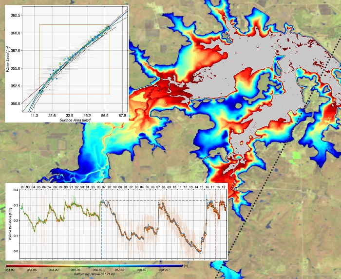
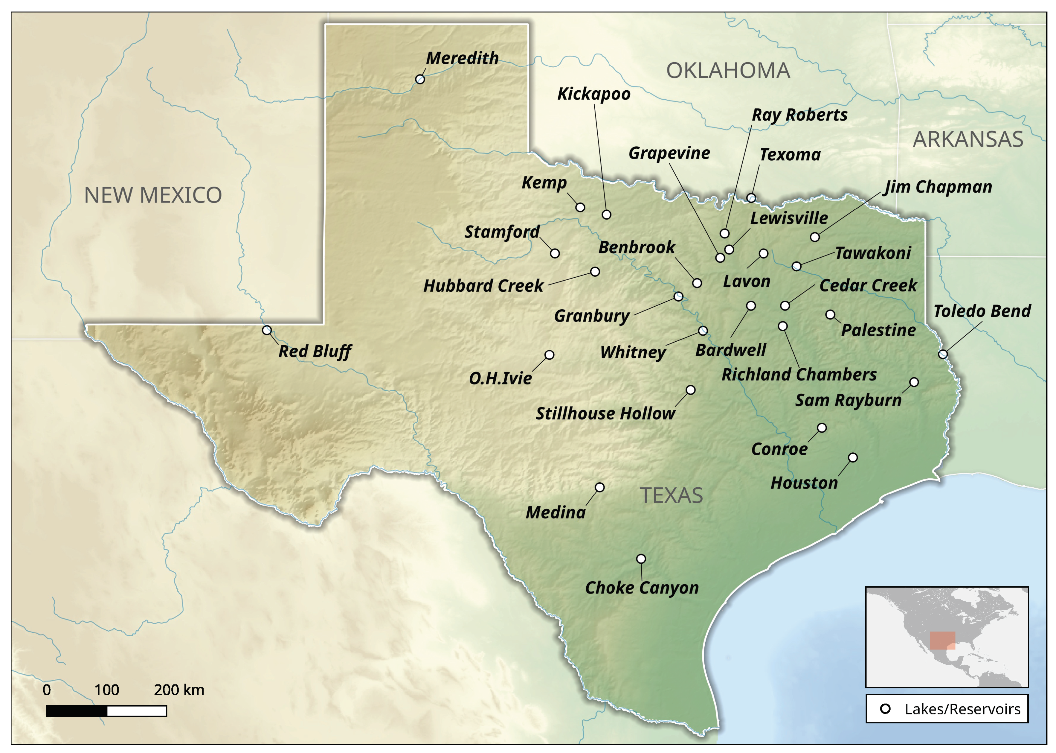
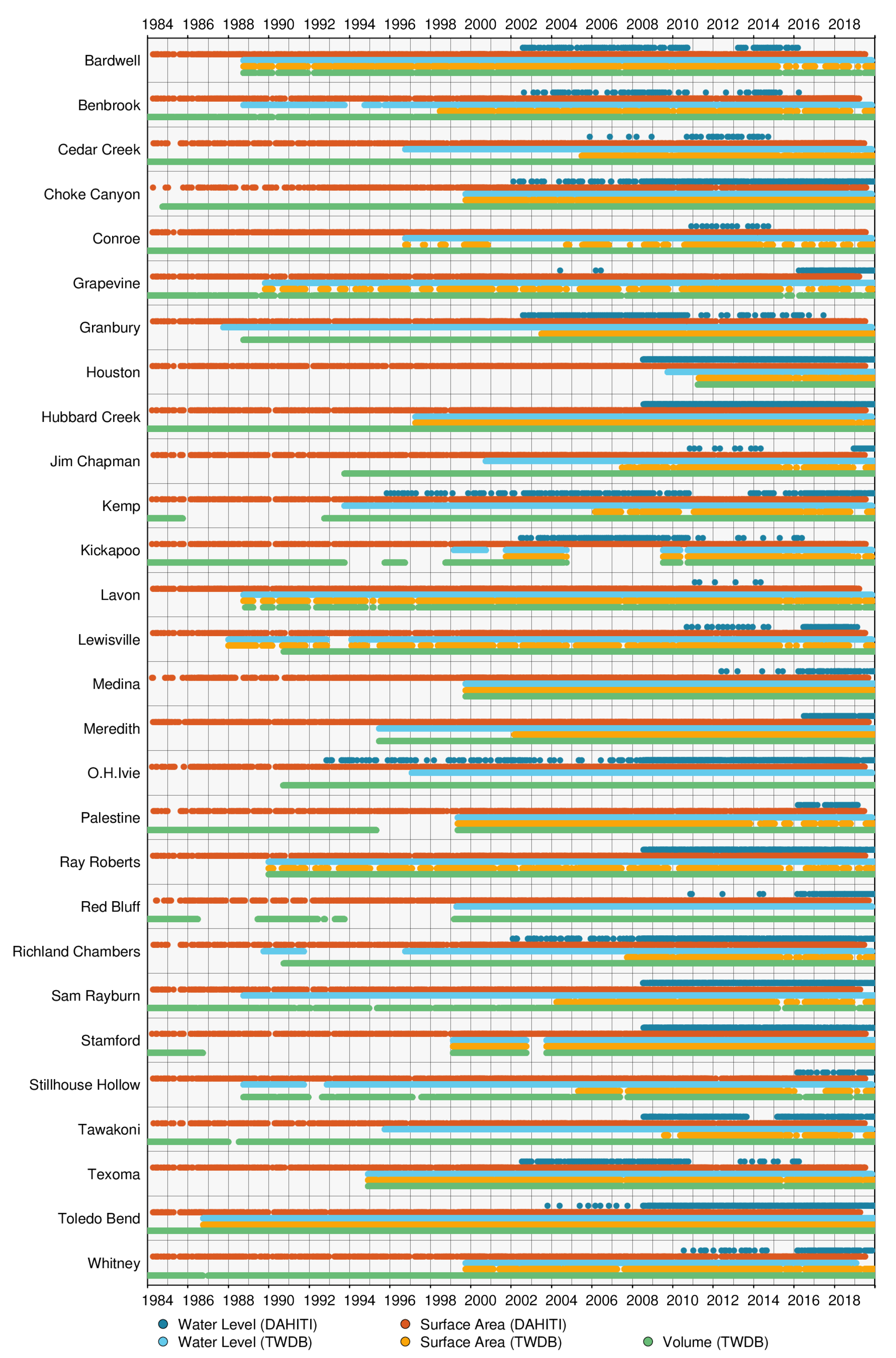
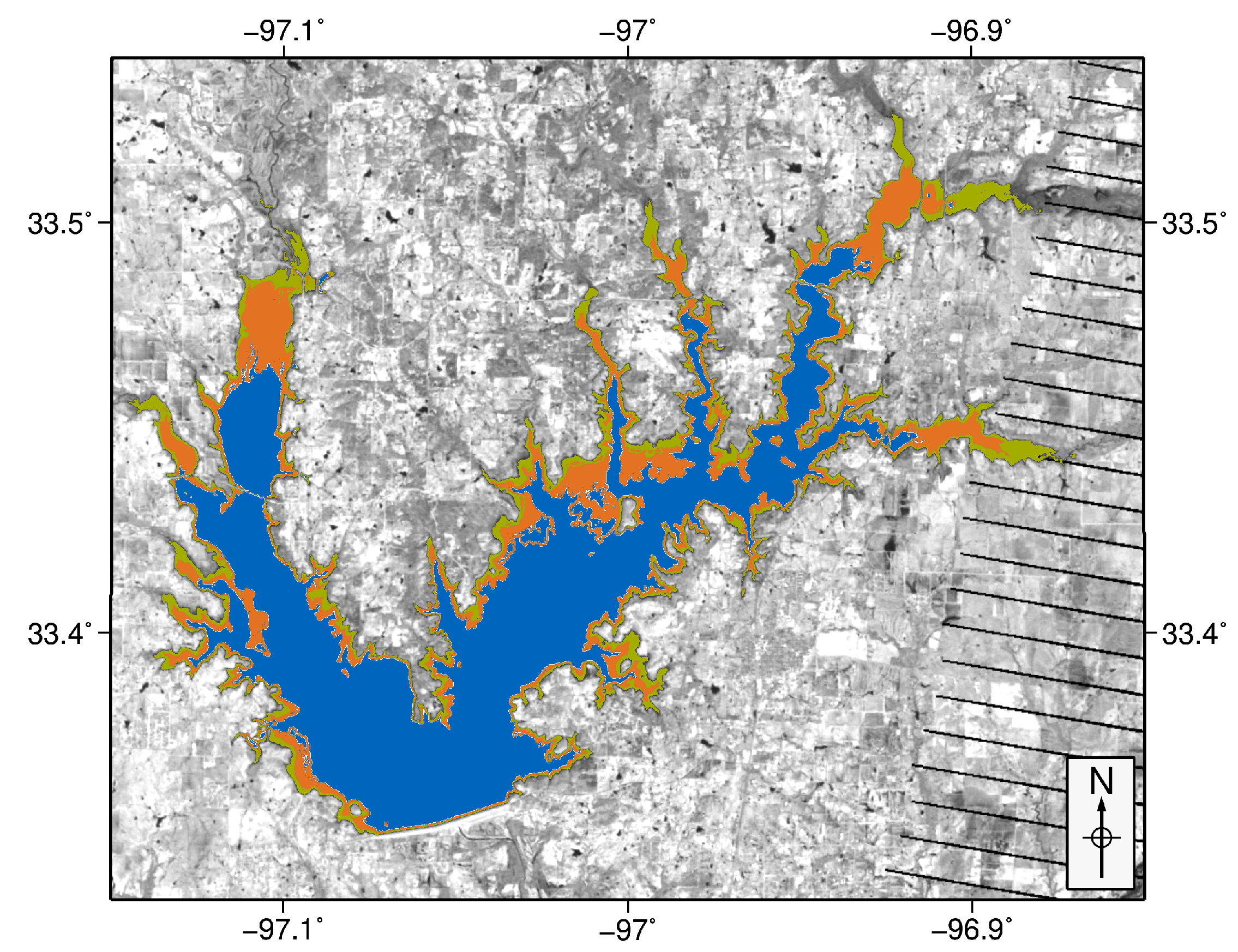
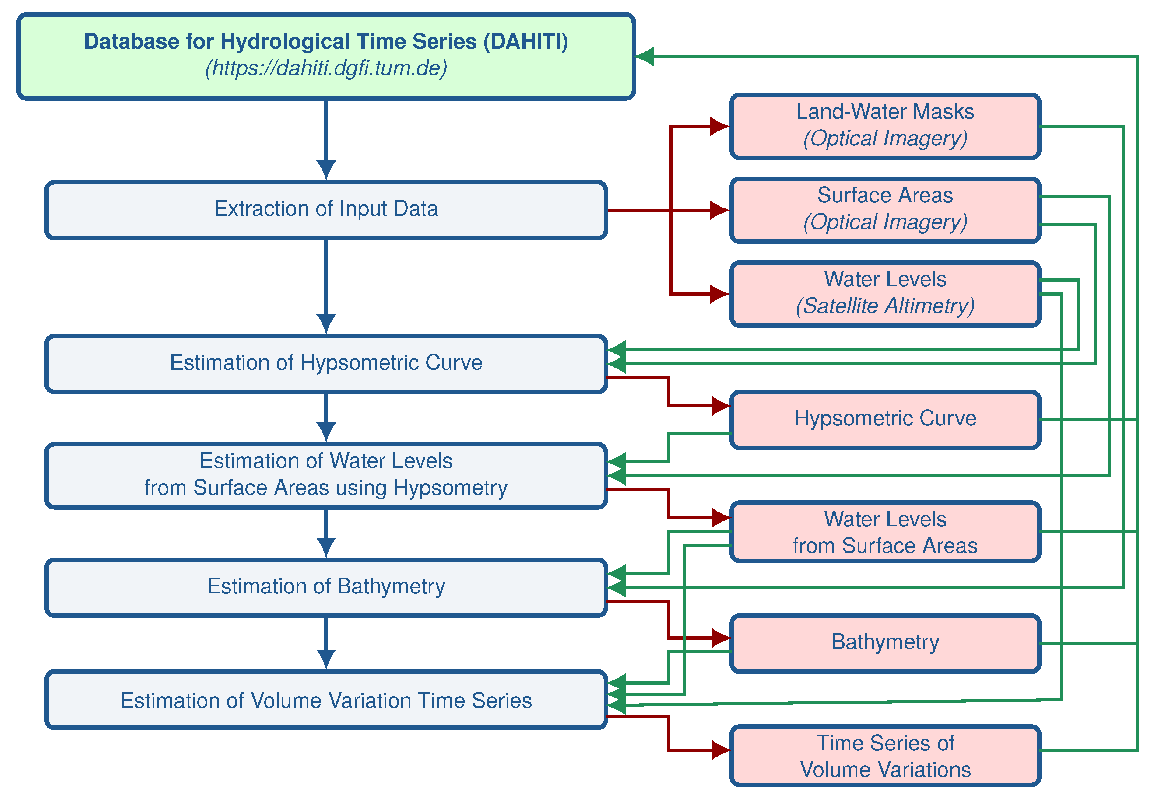
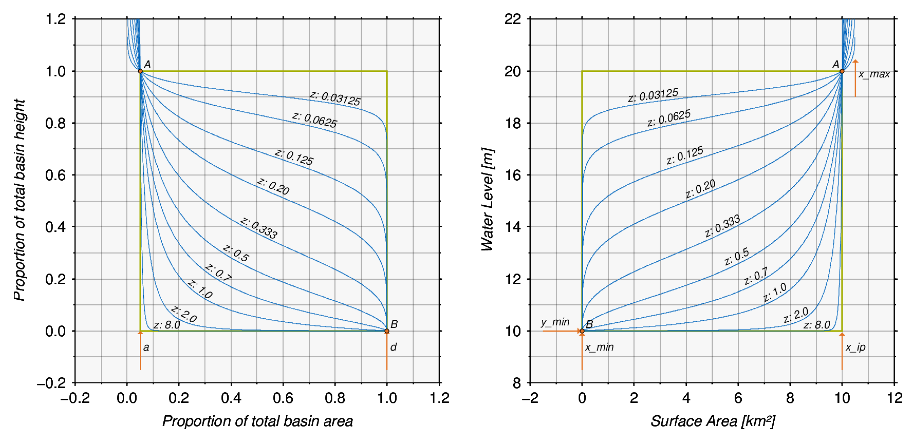
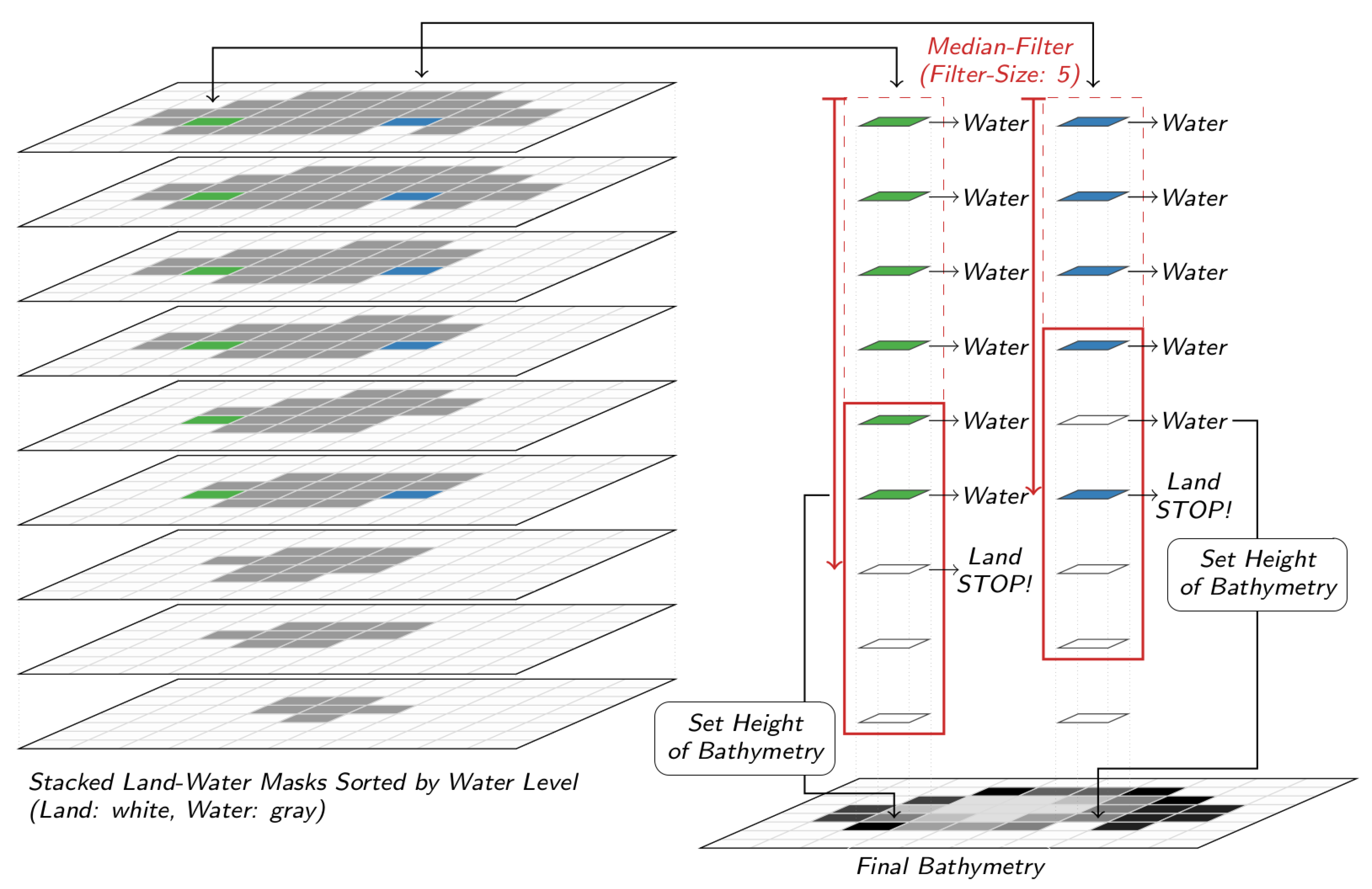
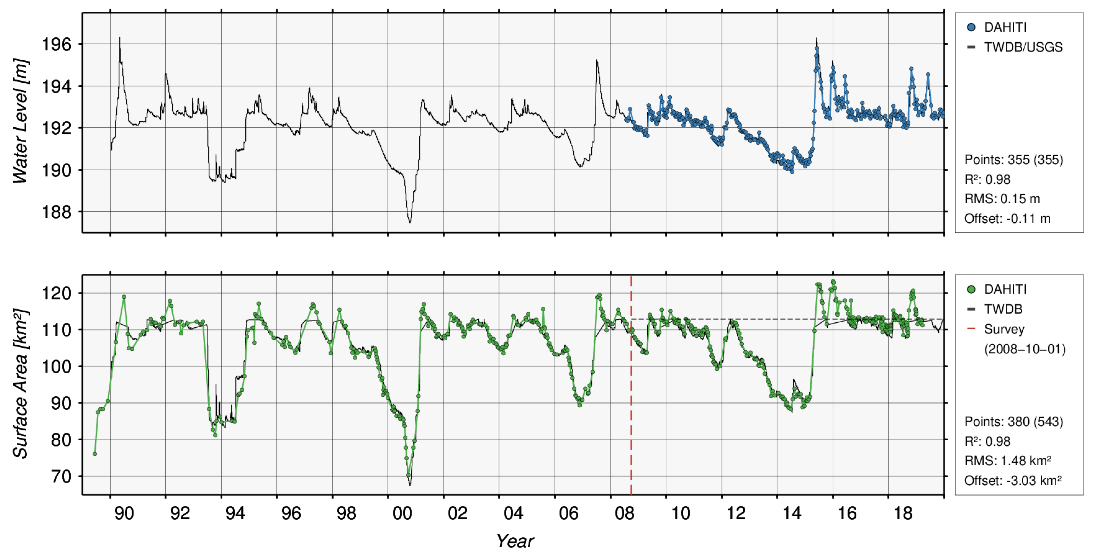
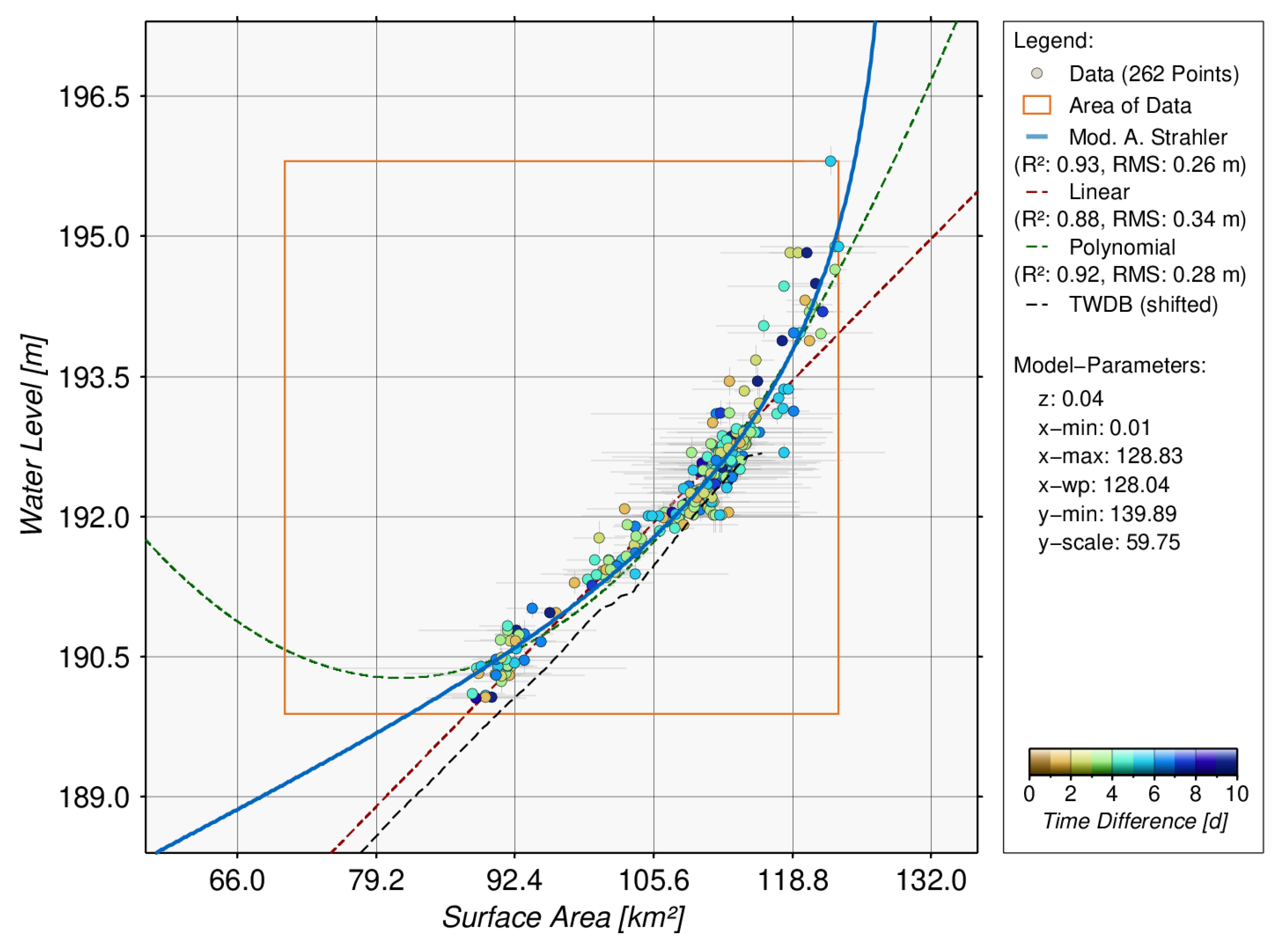
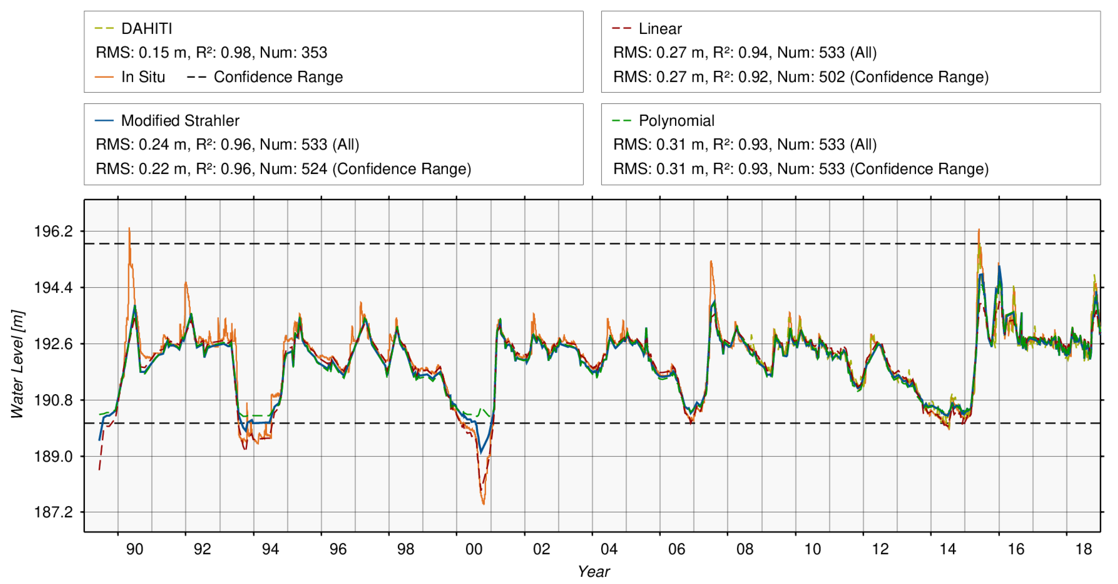
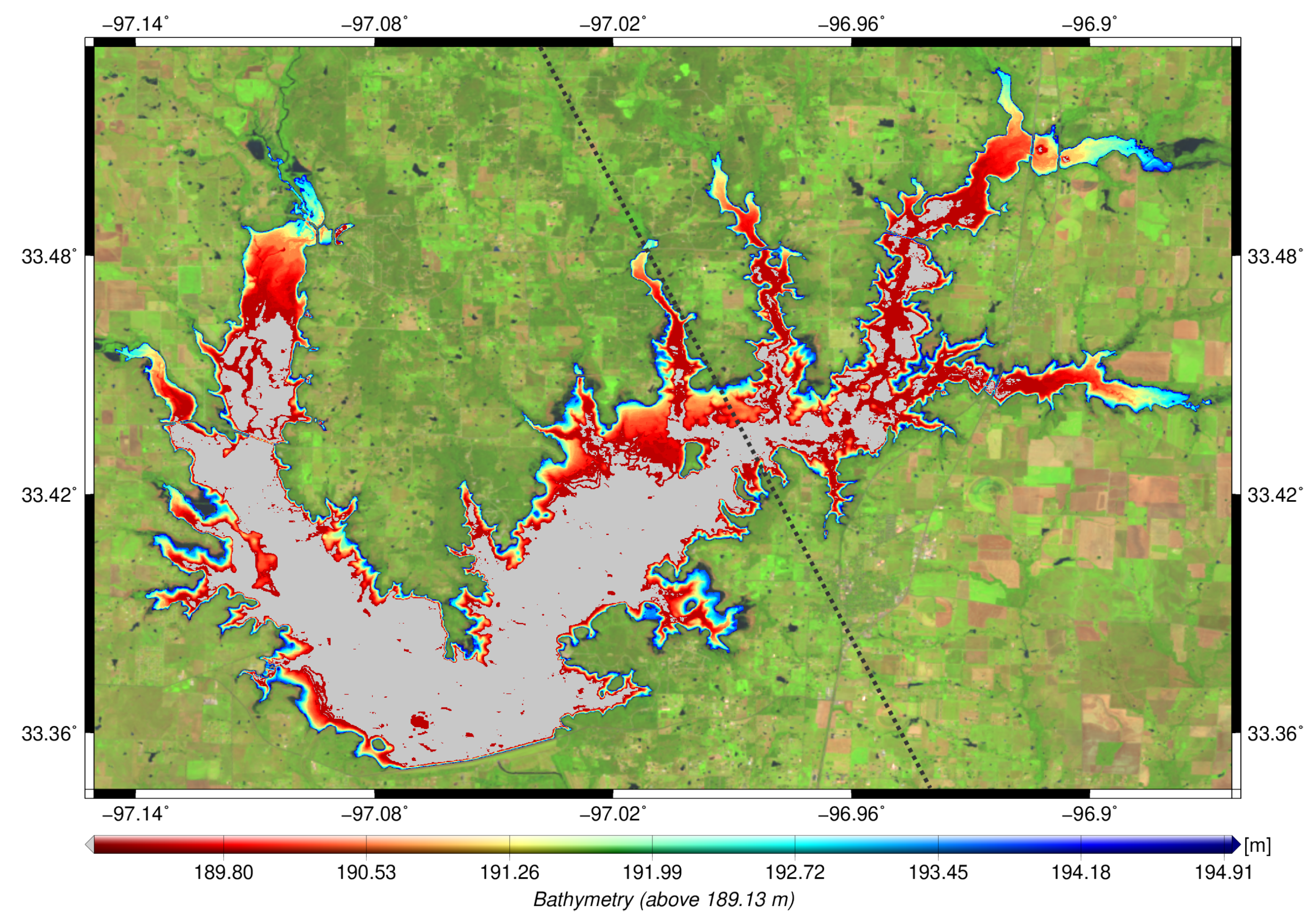
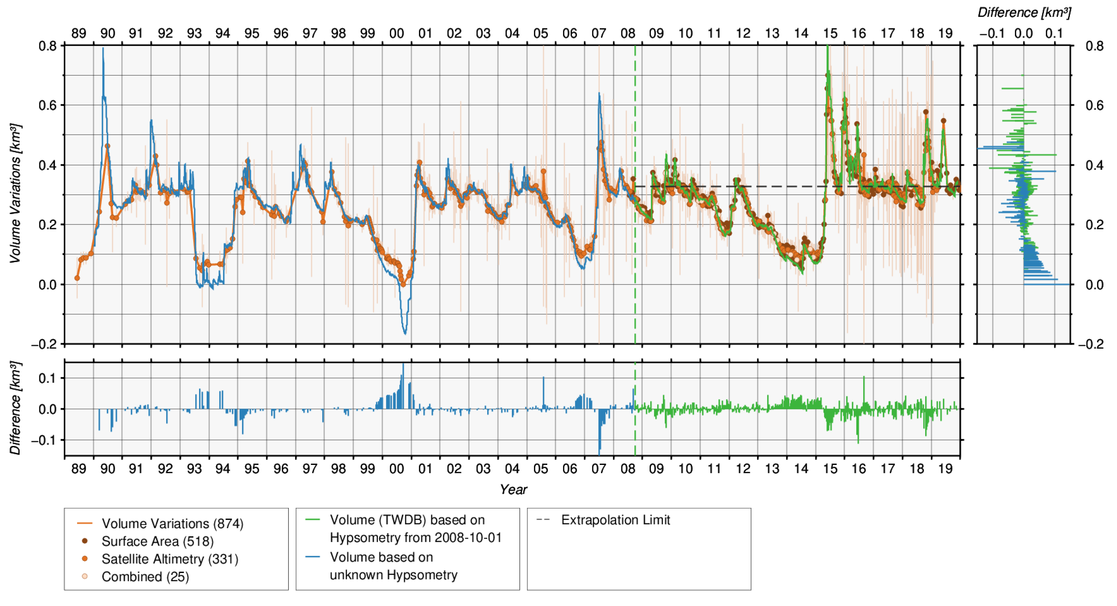
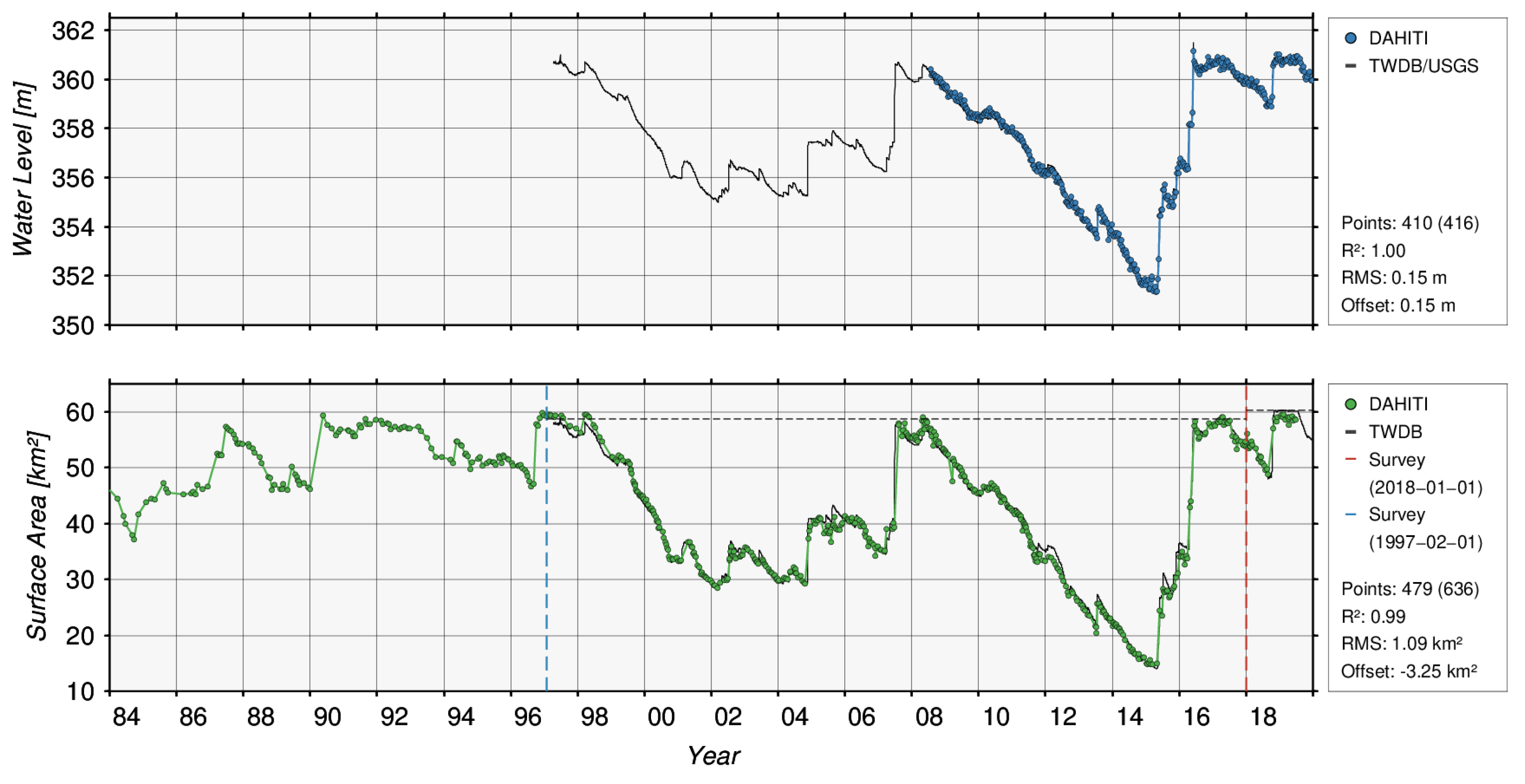
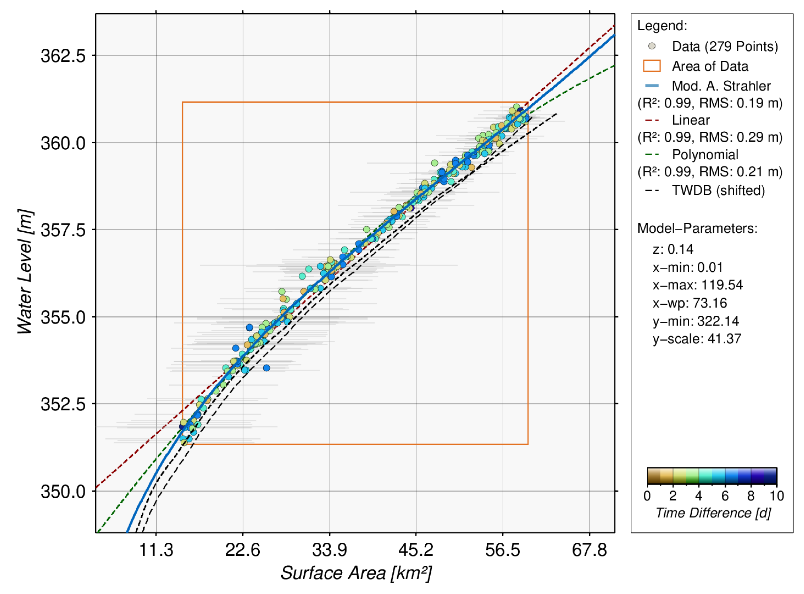
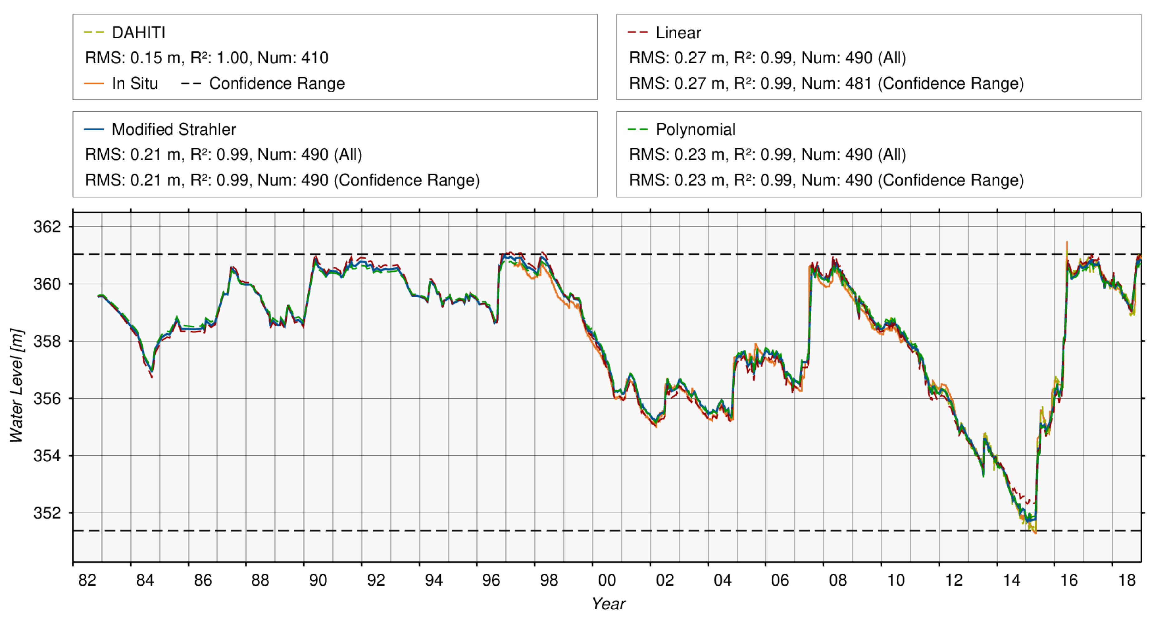
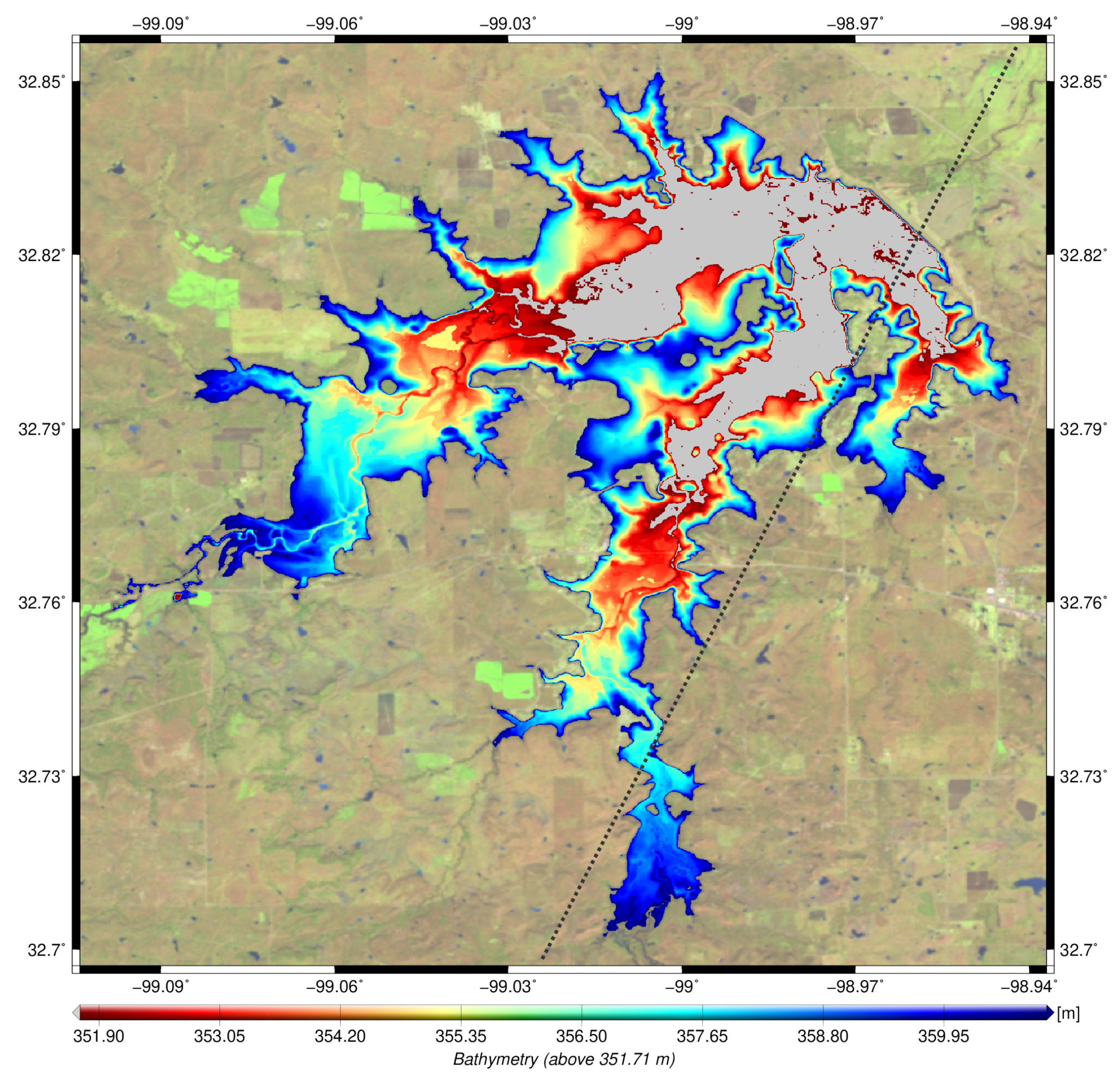
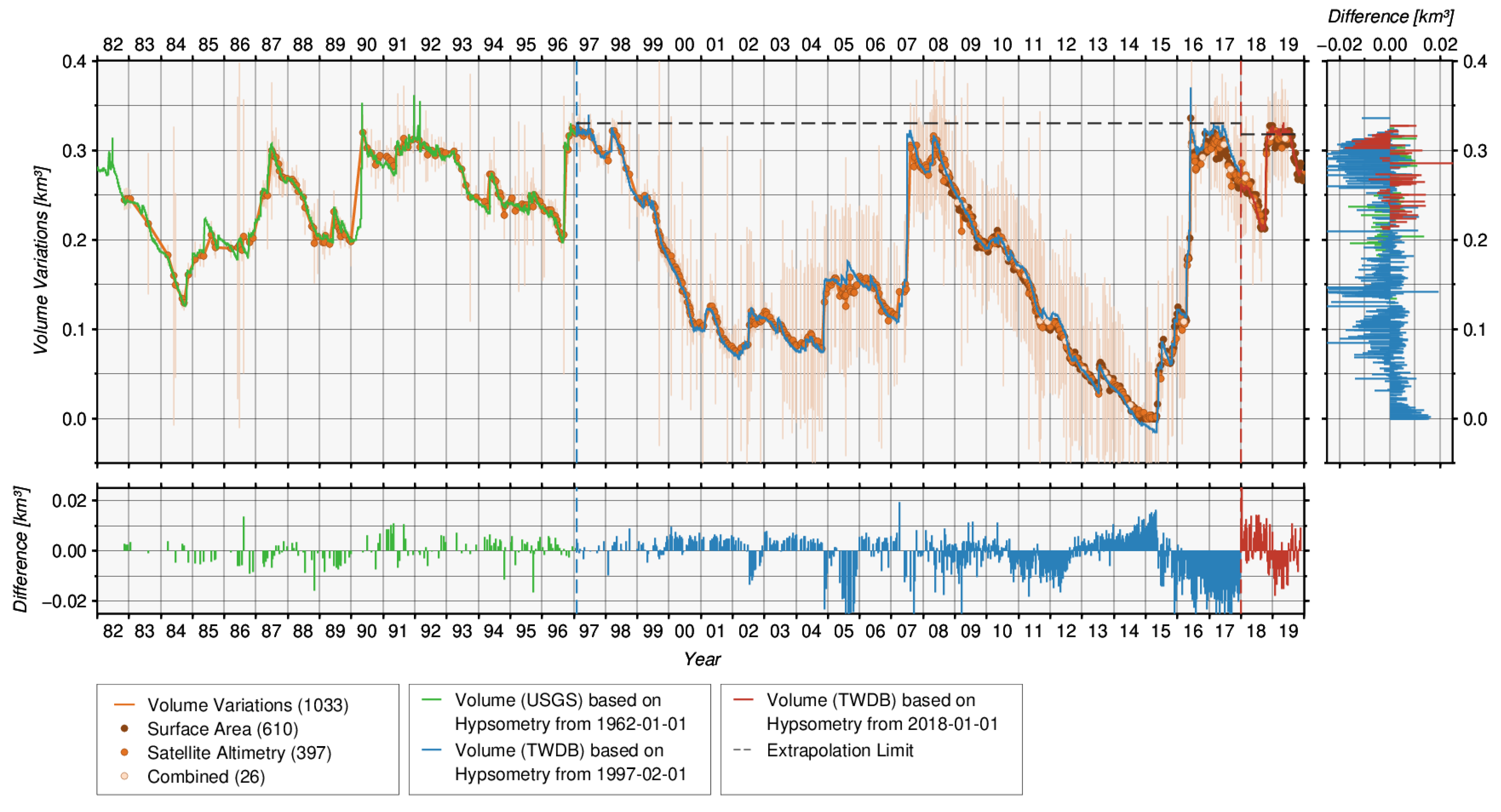
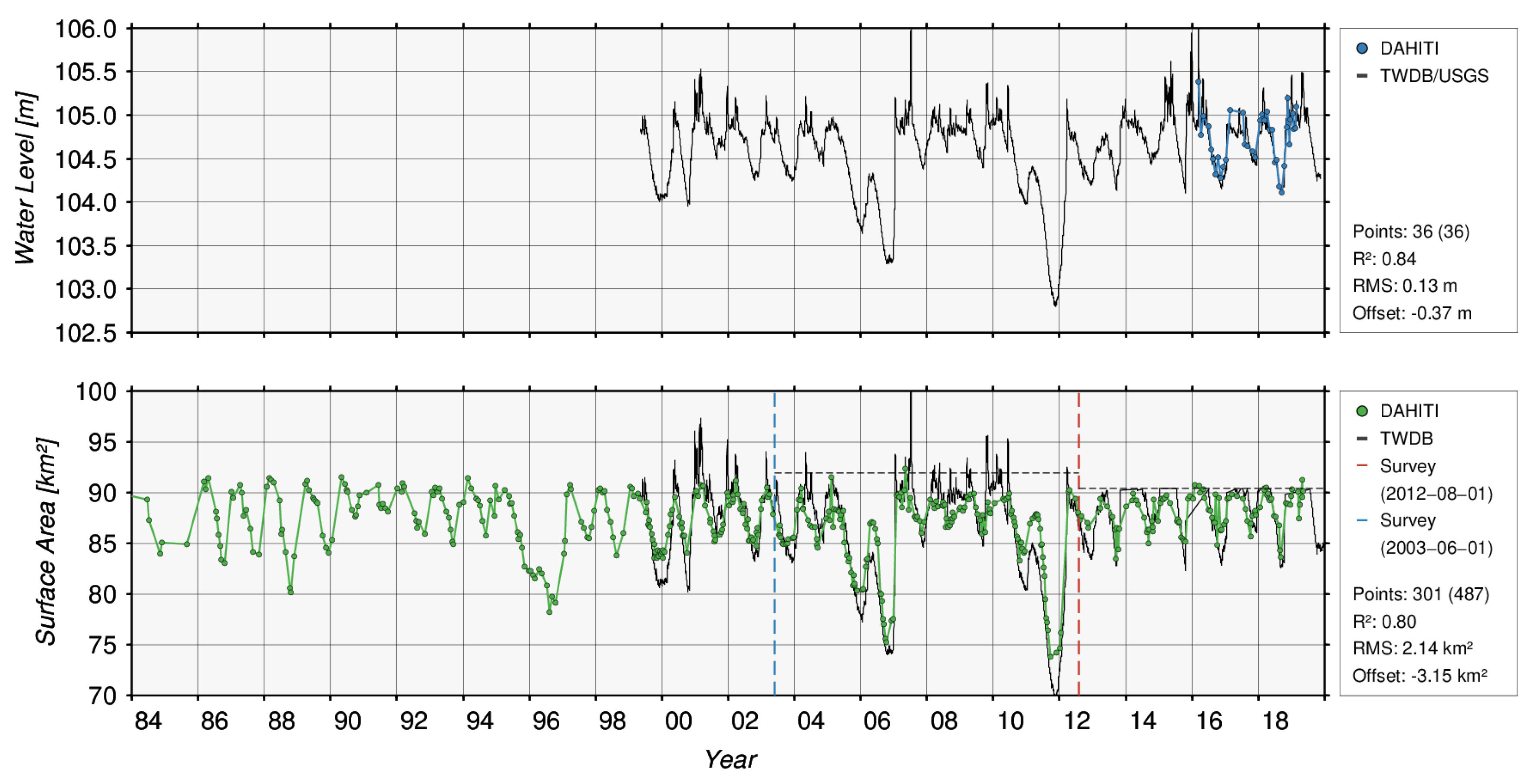
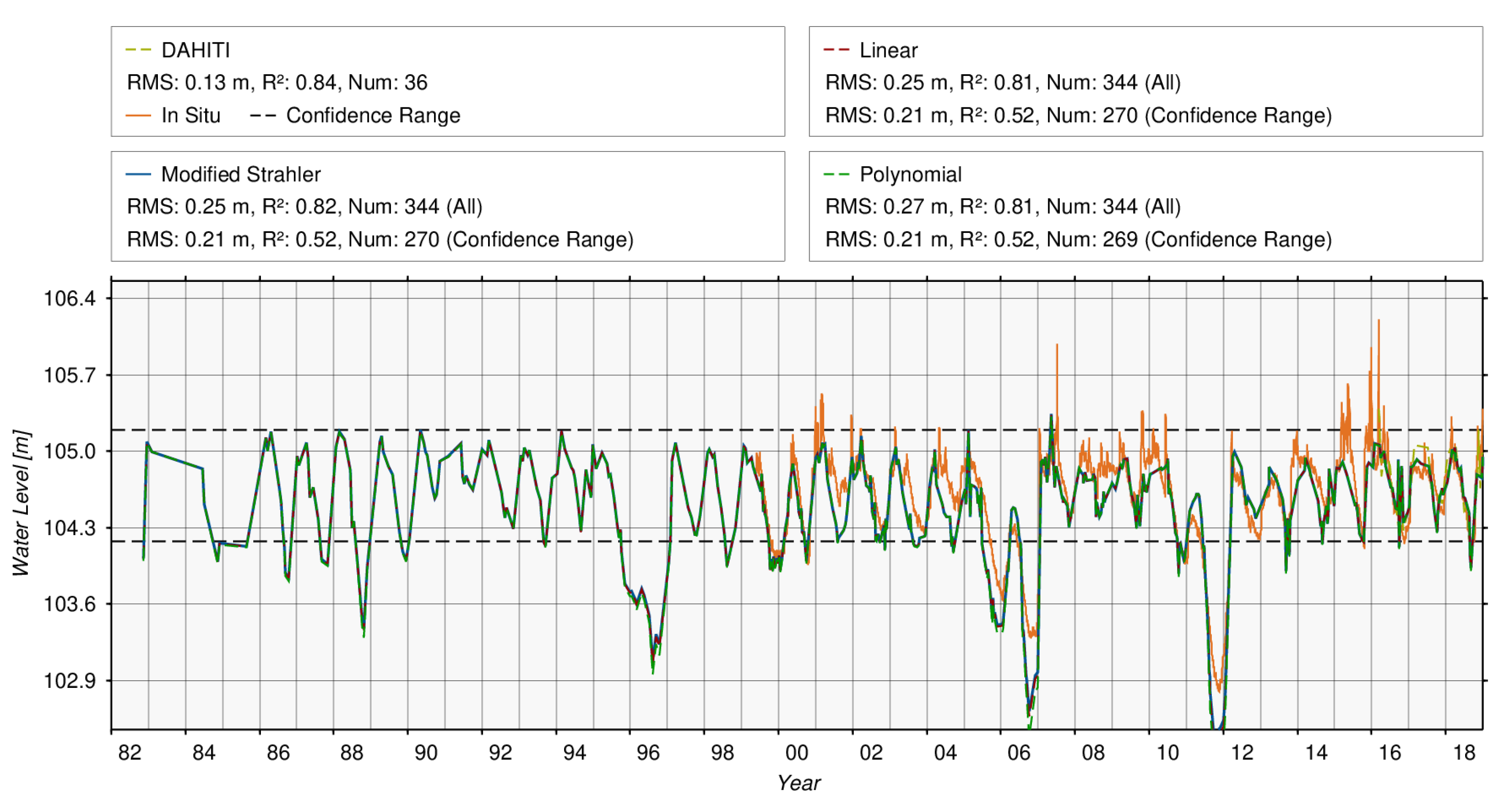
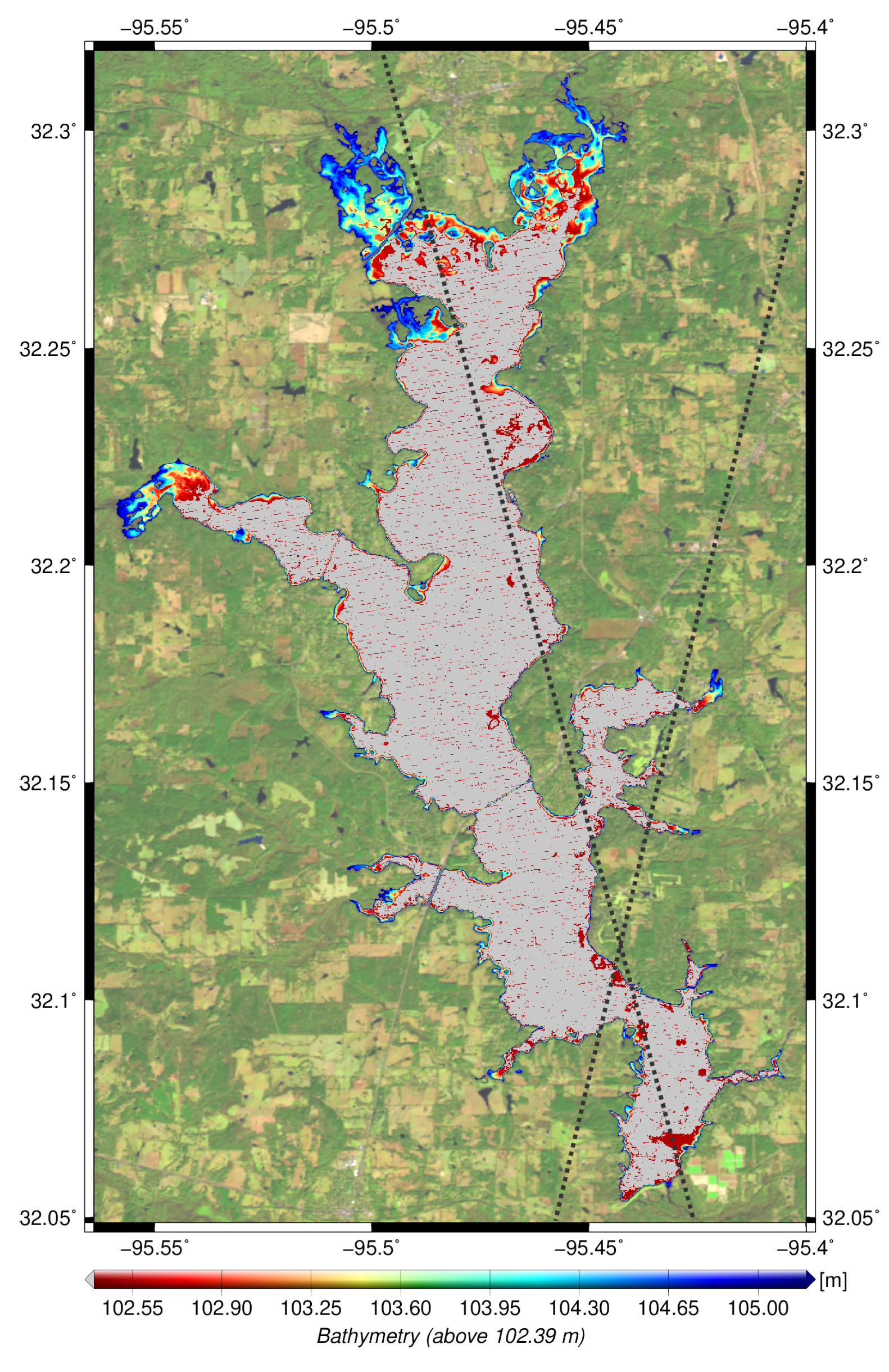
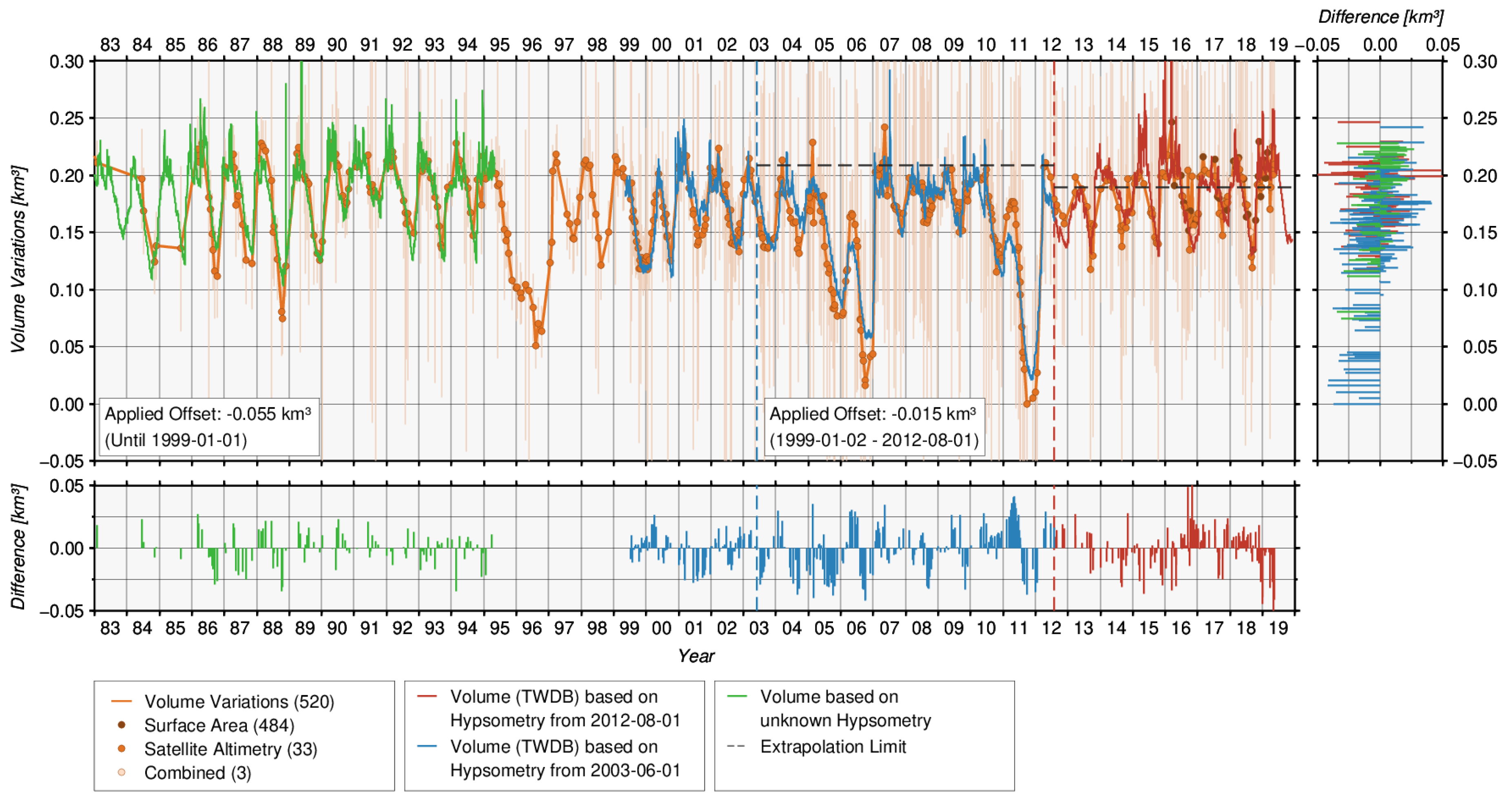
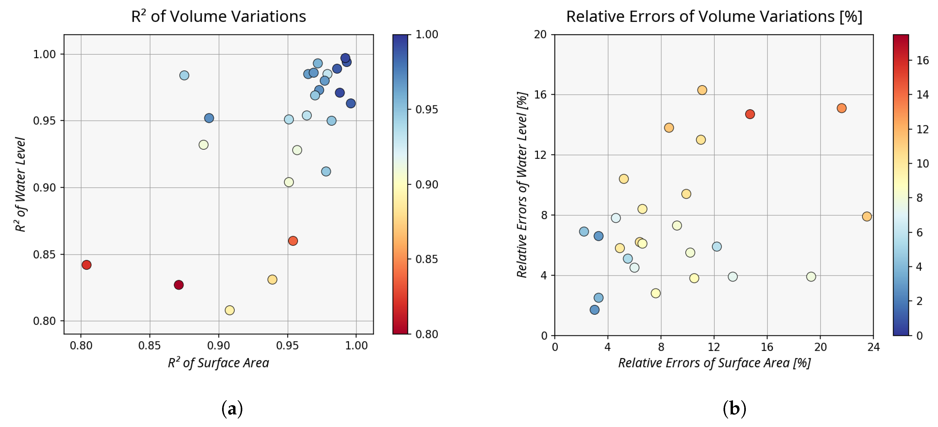
Table 1.
List of water bodies and characteristics derived from available in-situ data.
| Target Name (ID) | Water Level [m] | Surface Area [km] | Volume [km] | ||||||
|---|---|---|---|---|---|---|---|---|---|
| Min. | Max. | Var. | Min. | Max. | Var. | Min. | Max. | Var. | |
| Bardwell (10317) | 126.70 | 134.32 | 7.62 | 10.37 | 13.00 | 2.63 | 0.038 | 0.062 | 0.024 |
| Benbrook (10147) | 206.09 | 218.42 | 12.33 | 9.10 | 14.71 | 5.61 | 0.000 | 0.116 | 0.116 |
| Cedar Creek (13002) | 95.77 | 98.54 | 2.77 | 102.22 | 132.93 | 30.71 | 0.000 | 0.877 | 0.877 |
| Choke Canyon (13116) | 58.41 | 68.11 | 9.70 | 42.80 | 102.17 | 59.37 | 0.006 | 0.956 | 0.950 |
| Conroe (13132) | 58.74 | 62.76 | 4.02 | 60.69 | 76.99 | 16.31 | 0.000 | 0.647 | 0.647 |
| Grapevine (13061) | 159.04 | 171.60 | 12.56 | 19.19 | 27.15 | 7.96 | 0.000 | 0.248 | 0.248 |
| Granbury (13190) | 207.72 | 211.21 | 3.49 | 18.70 | 34.52 | 15.82 | 0.089 | 0.175 | 0.086 |
| Houston (8850) | 11.08 | 15.93 | 4.86 | 33.18 | 45.66 | 12.47 | 0.103 | 0.198 | 0.095 |
| Hubbard Creek (10272) | 351.12 | 361.33 | 10.21 | 17.21 | 63.48 | 46.27 | 0.005 | 0.529 | 0.524 |
| Jim Chapman (10505) | 128.63 | 136.71 | 8.07 | 37.95 | 72.67 | 34.72 | 0.098 | 0.568 | 0.470 |
| Kemp (13146) | 341.07 | 350.42 | 9.35 | 15.76 | 62.15 | 46.39 | 0.002 | 0.485 | 0.483 |
| Kickapoo (10279) | 313.77 | 319.24 | 5.47 | 10.01 | 23.73 | 13.72 | 0.000 | 0.146 | 0.146 |
| Lavon (13043) | 144.74 | 153.79 | 9.05 | 45.24 | 87.48 | 42.24 | 0.171 | 0.530 | 0.359 |
| Lewisville (11327) | 154.55 | 163.61 | 9.06 | 62.81 | 109.97 | 47.16 | 0.345 | 1.326 | 0.981 |
| Medina (13183) | 296.39 | 326.59 | 30.20 | 2.46 | 26.79 | 24.33 | 0.009 | 0.371 | 0.363 |
| Meredith (12977) | 865.37 | 886.61 | 21.24 | 6.35 | 33.79 | 27.43 | 0.020 | 0.539 | 0.519 |
| O.H.Ivie (10271) | 457.97 | 473.21 | 15.25 | n.a. | n.a. | n.a. | 0.073 | 0.709 | 0.636 |
| Palestine (13077) | 103.17 | 106.58 | 3.41 | 72.74 | 105.56 | 32.82 | 0.000 | 0.639 | 0.639 |
| Ray Roberts (10146) | 187.58 | 196.43 | 8.86 | 70.52 | 115.93 | 45.41 | 0.490 | 1.449 | 0.958 |
| Red Bluff (13158) | 851.73 | 863.29 | 11.56 | n.a. | n.a. | n.a. | 0.013 | 0.180 | 0.167 |
| Richland Chambers (8814) | 92.55 | 96.62 | 4.08 | 133.31 | 175.32 | 42.00 | 0.845 | 1.497 | 0.652 |
| Sam Rayburn (10246) | 45.95 | 53.33 | 7.38 | 308.62 | 455.57 | 146.96 | 0.000 | 4.017 | 4.017 |
| Stamford (10274) | 426.54 | 434.64 | 8.10 | 3.98 | 28.12 | 24.14 | 0.000 | 0.107 | 0.107 |
| Stillhouse Hollow (13157) | 182.88 | 202.38 | 19.50 | 16.71 | 27.22 | 10.51 | 0.170 | 0.301 | 0.131 |
| Tawakoni (8813) | 129.52 | 134.59 | 5.07 | 104.39 | 151.05 | 46.66 | 0.000 | 1.371 | 1.391 |
| Texoma (13141) | 185.35 | 196.80 | 11.45 | 237.56 | 323.47 | 85.91 | 2.385 | 3.786 | 1.402 |
| Toledo Bend (10247) | 48.62 | 53.10 | 4.48 | 510.13 | 782.16 | 272.03 | 0.000 | 6.041 | 6.041 |
| Whitney (13102) | 157.49 | 171.09 | 13.60 | 53.05 | 93.76 | 40.71 | 0.000 | 2.433 | 2.433 |
1 Based on water levels, surface areas and volumes provided by TWDB.
Table 2.
Quality assessment for 28 selected water bodies. For each water body, the validation results with in-situ data are shown for the used water levels from altimetry and surface areas from optical images (number of data sets, Pearson correlation, RMSE, relative error). Additionally, the resulting quality of the estimated hypsometry model is given (number of data sets, Spearman correlation, RMSE). Finally, the validation results for the volume variations are presented (number of data sets, Pearson correlation, RMSE, relative error, absolute error, offset).
| Target Name (ID) | Altimetry | Surface Area | Hypsometry | Volume | |||||||||||||||
|---|---|---|---|---|---|---|---|---|---|---|---|---|---|---|---|---|---|---|---|
| vs. In-Situ [m] | vs. In-Situ [km] | vs. In-Situ [km] | |||||||||||||||||
| # | R | RMSE | rel% | # | R | RMSE | rel% | # | R | RMSE | # | R | RMSE | rel% | abs% | Offset | |||
| Bardwell (10317) | 42 | 0.83 | 0.30 | 13.8 | 427 | 0.94 | 0.13 | 8.6 | 44 | 0.67 | 0.32 | 514 | 0.88 | 0.002 | 11.4 | 2.9 | −0.038 | ||
| Benbrook (10147) | 67 | 0.91 | 0.43 | 10.4 | 349 | 0.98 | 0.18 | 5.2 | 44 | 0.86 | 0.42 | 591 | 0.95 | 0.004 | 10.2 | 3.2 | −0.054 | ||
| Cedar Creek (13002) | 30 | 0.81 | 0.28 | 13.0 | 171 | 0.91 | 2.27 | 11.0 | 24 | 0.83 | 0.28 | 473 | 0.89 | 0.023 | 10.3 | 2.7 | −0.537 | ||
| Choke Canyon (13116) | 331 | 0.99 | 0.20 | 2.5 | 244 | 0.99 | 1.67 | 3.3 | 162 | 0.97 | 0.47 | 668 | 0.99 | 0.022 | 3.9 | 2.4 | −0.173 | ||
| Conroe (13132) | 14 | 0.83 | 0.26 | 14.7 | 92 | 0.87 | 1.01 | 14.7 | 5 | 0.94 | 0.15 | 398 | 0.80 | 0.015 | 14.9 | 2.8 | −0.310 | ||
| Grapevine (13061) | 78 | 0.95 | 0.29 | 6.2 | 360 | 0.96 | 0.39 | 6.4 | 104 | 0.87 | 0.42 | 652 | 0.93 | 0.008 | 10.2 | 3.2 | −0.121 | ||
| Granbury (13190) | 102 | 0.90 | 0.24 | 9.4 | 281 | 0.95 | 1.07 | 9.9 | 166 | 0.83 | 0.28 | 554 | 0.91 | 0.005 | 10.3 | 3.1 | −0.102 | ||
| Houston (8850) | 371 | 0.86 | 0.14 | 16.3 | 43 | 0.95 | 1.03 | 11.1 | 136 | 0.76 | 0.17 | 389 | 0.84 | 0.005 | 11.1 | 2.7 | −0.109 | ||
| Hubbard Creek (10272) | 410 | 1.00 | 0.15 | 1.7 | 479 | 0.99 | 1.09 | 3.0 | 279 | 0.99 | 0.20 | 1021 | 0.99 | 0.008 | 2.8 | 2.0 | −0.071 | ||
| Jim Chapman (10505) | 19 | 0.98 | 0.29 | 5.8 | 128 | 0.98 | 1.45 | 4.9 | 25 | 0.90 | 0.53 | 347 | 0.93 | 0.034 | 9.9 | 6.4 | −0.063 | ||
| Kemp (13146) | 156 | 0.95 | 0.41 | 5.9 | 230 | 0.89 | 5.16 | 12.2 | 188 | 0.94 | 0.46 | 687 | 0.97 | 0.015 | 5.7 | 4.2 | −0.043 | ||
| Kickapoo (10279) | 17 | 0.96 | 0.19 | 6.9 | 258 | 1.00 | 0.27 | 2.2 | 52 | 0.92 | 0.28 | 486 | 0.99 | 0.003 | 4.4 | 2.9 | −0.029 | ||
| Lavon (13043) | 6 | 0.98 | 0.15 | 6.1 | 560 | 0.96 | 1.75 | 6.6 | 4 | 0.97 | 0.16 | 566 | 0.96 | 0.019 | 8.7 | 3.7 | −0.200 | ||
| Lewisville (11327) | 32 | 0.95 | 0.24 | 7.8 | 381 | 0.98 | 1.36 | 4.6 | 50 | 0.89 | 0.35 | 565 | 0.95 | 0.029 | 7.1 | 2.3 | −0.442 | ||
| Medina (13183) | 52 | 0.99 | 0.78 | 3.8 | 239 | 0.99 | 1.07 | 10.5 | 37 | 0.98 | 0.37 | 289 | 0.99 | 0.016 | 8.9 | 5.0 | −0.079 | ||
| Meredith (12977) | 43 | 0.97 | 0.30 | 6.6 | 671 | 0.99 | 0.65 | 3.3 | 85 | 0.96 | 0.35 | 890 | 0.99 | 0.014 | 2.9 | 2.5 | −0.010 | ||
| O.H.Ivie (10271) | 413 | 0.99 | 0.35 | 3.4 | — | — | — | — | 364 | 0.99 | 0.42 | 1029 | 0.99 | 0.029 | 6.1 | 4.4 | −0.105 | ||
| Palestine (13077) | 36 | 0.84 | 0.13 | 15.1 | 301 | 0.80 | 2.14 | 21.6 | 32 | 0.64 | 0.17 | 475 | 0.82 | 0.017 | 13.0 | 3.3 | −0.264 | ||
| Ray Roberts (10146) | 353 | 0.98 | 0.15 | 4.5 | 380 | 0.98 | 1.48 | 6.0 | 262 | 0.93 | 0.26 | 867 | 0.97 | 0.025 | 7.2 | 1.8 | −0.647 | ||
| Red Bluff (13158) | 48 | 0.99 | 0.15 | 3.6 | — | — | — | — | 83 | 0.96 | 0.19 | 599 | 0.98 | 0.007 | 6.0 | 4.0 | −0.037 | ||
| Richland Chambers (8814) | 400 | 0.97 | 0.15 | 5.1 | 146 | 0.97 | 1.93 | 5.5 | 233 | 0.95 | 0.21 | 824 | 0.97 | 0.024 | 5.4 | 1.7 | −0.879 | ||
| Sam Rayburn (10246) | 408 | 0.98 | 0.16 | 3.9 | 208 | 0.88 | 11.82 | 19.3 | 203 | 0.88 | 0.38 | 774 | 0.94 | 0.096 | 7.8 | 2.4 | −2.096 | ||
| Stamford (10274) | 351 | 0.99 | 0.21 | 3.9 | 364 | 0.97 | 1.55 | 13.4 | 227 | 0.92 | 0.38 | 717 | 0.97 | 0.004 | 7.3 | 4.5 | −0.011 | ||
| Stillhouse Hollow (13157) | 30 | 0.99 | 0.13 | 2.8 | 208 | 0.97 | 0.59 | 7.6 | 32 | 0.91 | 0.35 | 463 | 0.96 | 0.007 | 8.8 | 2.1 | −0.193 | ||
| Tawakoni (8813) | 276 | 0.93 | 0.20 | 8.4 | 111 | 0.96 | 2.14 | 6.6 | 157 | 0.83 | 0.26 | 721 | 0.91 | 0.032 | 9.5 | 2.7 | −0.687 | ||
| Texoma (13141) | 87 | 0.95 | 0.22 | 7.3 | 416 | 0.95 | 4.83 | 9.2 | 109 | 0.84 | 0.39 | 510 | 0.94 | 0.058 | 8.2 | 1.5 | −2.539 | ||
| Toledo Bend (10247) | 450 | 0.93 | 0.23 | 7.9 | 425 | 0.89 | 21.75 | 23.5 | 122 | 0.77 | 0.39 | 890 | 0.91 | 0.166 | 11.2 | 2.8 | −3.570 | ||
| Whitney (13102) | 53 | 0.97 | 0.26 | 5.5 | 334 | 0.97 | 2.48 | 10.2 | 68 | 0.95 | 0.32 | 562 | 0.95 | 0.023 | 8.1 | 2.9 | −0.348 | ||
| Minimum | 6 | 0.81 | 0.13 | 1.7 | 43 | 0.80 | 0.13 | 2.2 | 4 | 0.64 | 0.15 | 289 | 0.80 | 0.002 | 2.8 | 1.5 | −3.570 | ||
| Maximum | 450 | 1.00 | 0.78 | 16.3 | 671 | 1.00 | 21.75 | 23.5 | 364 | 0.99 | 0.53 | 1029 | 0.99 | 0.166 | 14.9 | 6.4 | −0.010 | ||
| Average | 166 | 0.94 | 0.25 | 7.2 | 300 | 0.95 | 2.74 | 9.2 | 117 | 0.89 | 0.32 | 625 | 0.94 | 0.025 | 8.3 | 3.1 | −0.491 | ||
1 Extrapolated validation data truncated; 2 Offset resulting from different hypsometry models applied.
© 2020 by the authors. Licensee MDPI, Basel, Switzerland. This article is an open access article distributed under the terms and conditions of the Creative Commons Attribution (CC BY) license (http://creativecommons.org/licenses/by/4.0/).
Share and Cite
MDPI and ACS Style
Schwatke, C.; Dettmering, D.; Seitz, F. Volume Variations of Small Inland Water Bodies from a Combination of Satellite Altimetry and Optical Imagery. Remote Sens. 2020, 12, 1606. https://doi.org/10.3390/rs12101606
AMA Style
Schwatke C, Dettmering D, Seitz F. Volume Variations of Small Inland Water Bodies from a Combination of Satellite Altimetry and Optical Imagery. Remote Sensing. 2020; 12(10):1606. https://doi.org/10.3390/rs12101606
Chicago/Turabian StyleSchwatke, Christian, Denise Dettmering, and Florian Seitz. 2020. "Volume Variations of Small Inland Water Bodies from a Combination of Satellite Altimetry and Optical Imagery" Remote Sensing 12, no. 10: 1606. https://doi.org/10.3390/rs12101606
Note that from the first issue of 2016, this journal uses article numbers instead of page numbers. See further details here.