Description of the UCAR/CU Soil Moisture Product


1
COSMIC, University Corporation for Atmospheric Research, Boulder, CO 80301, USA
2
Department of Geological Sciences, University of Colorado, Boulder, CO 80309, USA
*
Author to whom correspondence should be addressed.
Remote Sens. 2020, 12(10), 1558; https://doi.org/10.3390/rs12101558
Submission received: 14 April 2020
/
Revised: 12 May 2020
/
Accepted: 13 May 2020
/
Published: 14 May 2020
(This article belongs to the Special Issue Applications of GNSS Reflectometry for Earth Observation)
Abstract
:Currently, the ability to use remotely sensed soil moisture to investigate linkages between the water and energy cycles and for use in data assimilation studies is limited to passive microwave data whose temporal revisit time is 2–3 days or active microwave products with a much longer (>10 days) revisit time. This paper describes a dataset that provides soil moisture retrievals, which are gridded to 36 km, for the upper 5 cm of the soil surface at sparsely sampled 6-hour intervals for +/− 38 degrees latitude for 2017–present. Retrievals are derived from the Cyclone Global Navigation Satellite System (CYGNSS) constellation, which uses GNSS-Reflectometry to obtain L-band reflectivity observations over the Earth’s surface. The product was developed by calibrating CYGNSS reflectivity observations to soil moisture retrievals from NASA’s Soil Moisture Active Passive (SMAP) mission. Retrievals were validated against observations from 171 in-situ soil moisture probes, with a median unbiased root-mean-square error (ubRMSE) of 0.049 cm3 cm−3 (standard deviation = 0.026 cm3 cm−3) and median correlation coefficient of 0.4 (standard deviation = 0.27). For the same stations, the median ubRMSE between SMAP and in-situ observations was 0.045 cm3 cm−3 (standard deviation = 0.025 cm3 cm−3) and median correlation coefficient was 0.69 (standard deviation = 0.27). The UCAR/CU Soil Moisture Product is thus complementary to SMAP, albeit with a larger random noise component, providing soil moisture retrievals for applications that require faster revisit times than passive microwave remote sensing currently provides.

1. Introduction
Near-surface (0–5 cm) soil moisture data are used for a variety of applications, such as drought monitoring [1,2,3], flood forecasting [4,5], initializing climate models [6], numerical weather prediction [7], quantifying the linkages between the surface and atmospheric boundary layers [8,9,10], optimizing irrigation strategies [11], and predicting infectious disease transmission [12]. All of these applications require soil moisture data at different spatial and temporal scales. Due to its ability to retrieve soil moisture over large parts of the globe, satellite remote sensing is often used to provide these data. Most often, microwave instruments are used due to their ability to see through clouds and penetrate at least some amount of overlying vegetation. However, even the microwave sensor with the fastest revisit time (passive radiometer), is constrained to providing data every 2–3 days [13]. While for many soil moisture applications, such as climate model initialization, a 2–3 day repeat period is more than sufficient, other applications require a higher density of observations. For example, the quantification of soil moisture memory is limited to the time scale of observations [10]. Several ongoing efforts are also using soil moisture as a proxy for other quantities, such as rainfall [14,15] or evaporation [16,17], and having daily or sub-daily data would increase the success of these techniques.
A constellation of microwave instruments, the Cyclone Global Navigation Satellite System (CYGNSS), is currently on orbit over the tropics, and because it is a constellation with numerous satellites, it can provide data more frequently than currently possible using a single instrument alone [18]. Although not designed for soil moisture remote sensing, this paper describes a dataset [19] that has been developed from the CYGNSS constellation that provides soil moisture retrievals for the majority of the tropics (+/− 38 degrees latitude) at daily and sub-daily time steps. Here, we describe the algorithm, its assumptions, and validation of the retrievals using in-situ soil moisture observations. In regions where the algorithm performance is acceptable, the CYGNSS soil moisture retrievals could be used to augment existing soil moisture satellite data for the aforementioned applications that require data at a higher temporal resolution.
1.1. CYGNSS
The CYGNSS mission was launched in December 2016. A NASA Earth Ventures Mission, CYGNSS consists of eight small satellites that orbit the tropics with an inclination of 35 degrees [18]. CYGNSS was designed to retrieve ocean surface wind speed during hurricane intensification events, and, as such, the receivers and software were optimized for ocean surface remote sensing. Each of the CYGNSS satellites carries with it two downward-looking antennas and a Global Navigation Satellite System-Reflectometry (GNSS-R) receiver.
GNSS-R is a form of L-band bistatic radar that utilizes transmitted navigation signals as the signal source. GNSS is an umbrella term that encompasses constellations like the United States’ GPS, but also the EU’s Galileo, Russia’s GLONASS, China’s BeiDou, India’s IRNSS, and Japan’s QZSS. In total, there are over 80 GNSS satellites currently in orbit (32 of which are GPS satellites), with more being planned in the coming years. To date, GNSS-R most commonly utilizes right hand circular polarized (RHCP) L-band signals transmitted from GPS satellites, which upon reflection are predominantly left hand circular polarized (LHCP).
Because L-band signals are commonly used for near-surface (0–5 cm) soil moisture remote sensing (e.g., NASA’s Soil Moisture Active Passive (SMAP) or the European Space Agency’s Soil Moisture and Ocean Salinity (SMOS) missions [13,20]), there is significant interest in quantifying the sensitivity of spaceborne GNSS-R data to changes in soil moisture. There had been evidence of sensitivity during previous GNSS-R flight campaigns (e.g., [21,22,23,24,25]), though the first analyses investigating the sensitivity of spaceborne GNSS-R data to soil moisture were only done after the launch of TechDemoSat-1 (TDS-1) in 2014. TDS-1 carried the same GNSS-R receiver as is used by CYGNSS, and these preliminary investigations did show that there appeared to be some sensitivity of GNSS-R to soil moisture [26,27]. Due to the fact that TDS-1 only collected GNSS-R data for one out of every eight days, however, developing a full soil moisture retrieval algorithm was not attempted.
The sheer amount of data collected by CYGNSS has allowed for an empirical investigation into the sensitivity of spaceborne GNSS-R data to soil moisture. The dataset that we describe here is the result of a modified version of the methodology presented in [28]. The full dataset is available online [19]. The results presented here are the outcome of just one of several ongoing efforts investigating the potential of CYGNSS to retrieve soil moisture. Several of these efforts are also using SMAP retrievals as a reference data set, though differences arise in assumptions regarding gridding, open water masking, and vegetation considerations. For example, [29] assumed that the vast majority of CYGNSS observations have a coarse (>25 km) spatial resolution and spatially averaged the data under this assumption, whereas in the algorithm described here we assume a 3 km spatial resolution. The authors of [30] also used SMAP data for retrieval algorithm development, though also made considerations for changes in vegetation, and [31] incorporated surface roughness data from IceSat-2, neither of which do we do here. Both [29,32] scale their soil moisture retrievals by knowing a priori the maximum and minimum values of soil moisture for a particular region, which we also do not do here. Several other researchers are exploring machine learning techniques for CYGNSS soil moisture retrieval (e.g., [33,34]). Given the differences in validation data sets and time periods used for validation, it is difficult to directly compare the output of algorithms, though most have shown at least moderate success in retrieving soil moisture from CYGNSS.
1.2. GNSS-R Background
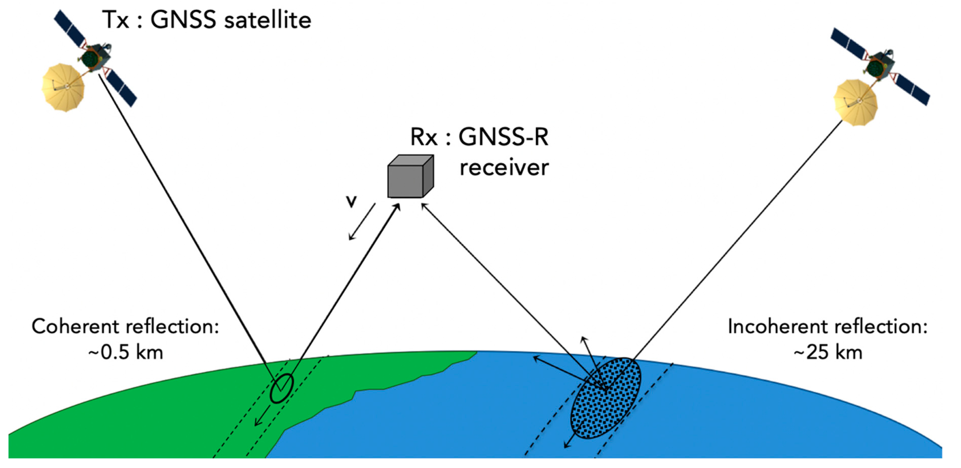
Unlike monostatic radar, which measures backscatter, GNSS-R measures the forward-scattered signal, which has reflected off of the surface of the Earth and back into space. Figure 1 presents a schematic of the signal geometry. A satellite in low Earth orbit, with a GNSS-R receiver onboard, has one or more downward-looking antennas, which record the forward-scattered signals. Information contained within the scattered signals can be related to land surface parameters, such as the surface roughness, dielectric constant of the soil, and vegetation properties.
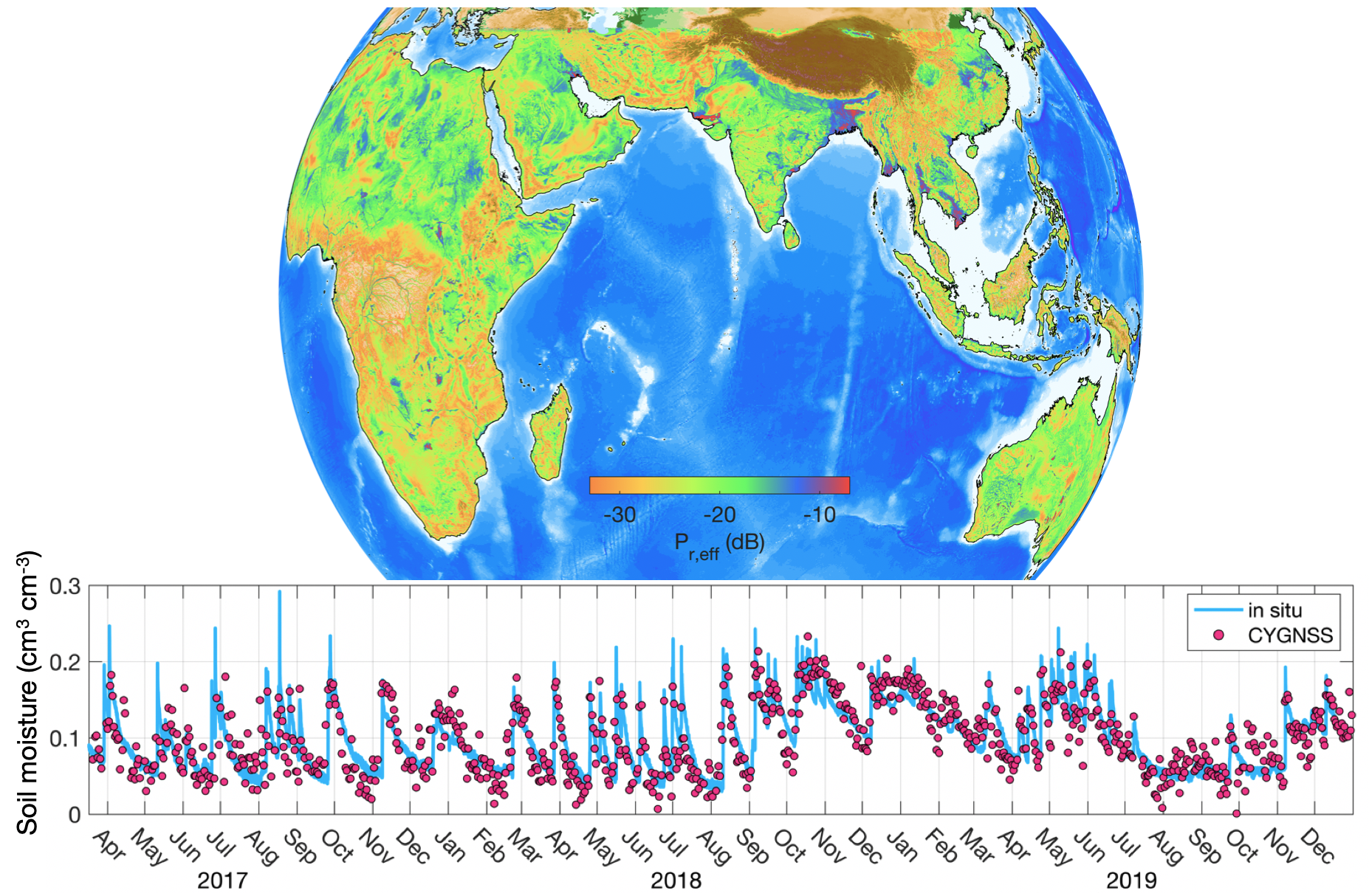
The point of reflection on the Earth’s surface is determined by the positions of the transmitting and receiving satellites. Because these positions are constantly changing, the reflection points are pseudo-randomly distributed on the Earth’s surface (see Figure 2a for examples), which is different than traditional remote-sensing techniques, which collect data in repeatable swaths. This means that, for a given point of the Earth’s surface, observations could be recorded one hour apart, and then there could be no observations for the next several hours, for example [35]. Observations are recorded at all times of day, again, unlike traditional remote-sensing techniques, which tend to observe a particular location at a particular time of day. The pseudo-random distribution of observations, over time, aggregate such that complete maps of the reflected signal can be made (Figure 2b).
The spatial resolution of the reflecting signal depends on the roughness of the surface at and near the reflection point [36]. Here, roughness includes possible contributions from many factors and not just the micro-scale roughness of the soil, such as roughness introduced from vegetation canopies, wind-roughened water, and macro-scale roughness from topography. If the surface is relatively rough, then the reflected signal is incoherent and comes from an area called the “glistening zone,” which is on the order of several kilometers (~25 km in the case of the ocean surface), though recent research is beginning to show that where incoherent scattering originates from over the land surface is highly dependent on the local topography and may not be definable with a simple 25-km radius [37]. If the surface is relatively smooth, then the reflected signal is coherent and comes from an area defined by the first Fresnel zone. For a low-Earth-orbiting GNSS-R satellite, this area is on the order of 0.5 km, though this also depends on incidence angle (0.33 km at 0 deg incidence, 1.3 km at 60 deg incidence) [38]. In practical terms, determining whether the reflecting surface is smooth enough to produce a coherent reflection is challenging, as surface roughness is an extremely difficult parameter to measure. Existing measurements show that surface roughness tends to be on the order of 2–3 cm [39,40,41], though surface roughness likely varies considerably on scales as large as the first Fresnel zone. There are also likely complications from macro-scale surface roughness due to topographic variations that are not well understood. Modelling efforts are beginning to shed light into the role of topography in GNSS-R signal scattering (e.g., [42,43]), with some studies showing that the sensitivity of the GNSS-R signal to soil moisture is relatively unaffected by complex topography [42].
In all likelihood, most signals are probably a combination of incoherent and coherent scattering. In the algorithm presented here, we ignore contributions from incoherent scattering. Assuming that the reflected signal is always coherent may lead to increased uncertainties in final soil moisture retrievals, though currently these uncertainties are not able to be quantified without a better knowledge of the precise conditions that lead to incoherence.
Due to the fact that CYGNSS was designed to be an ocean sensor, where the reflected signal is relatively weak, the processing software integrates the signal over a period of 1 s for each “observation.” During that time, the spacecraft has moved approximately 7 km, which means that the smallest along-track spatial resolution possible over land is 7 km, though the across track resolution could still be the theoretical 0.5 km. This results in the spatial footprint having a minimum size of 7 × 0.5 km, with the signal being smeared out along track (Figure 2a). In mid-2019, the CYGNSS integration time was decreased from 1 to 0.5 s, which means the minimum spatial footprint is currently 3.5 × 0.5 km.
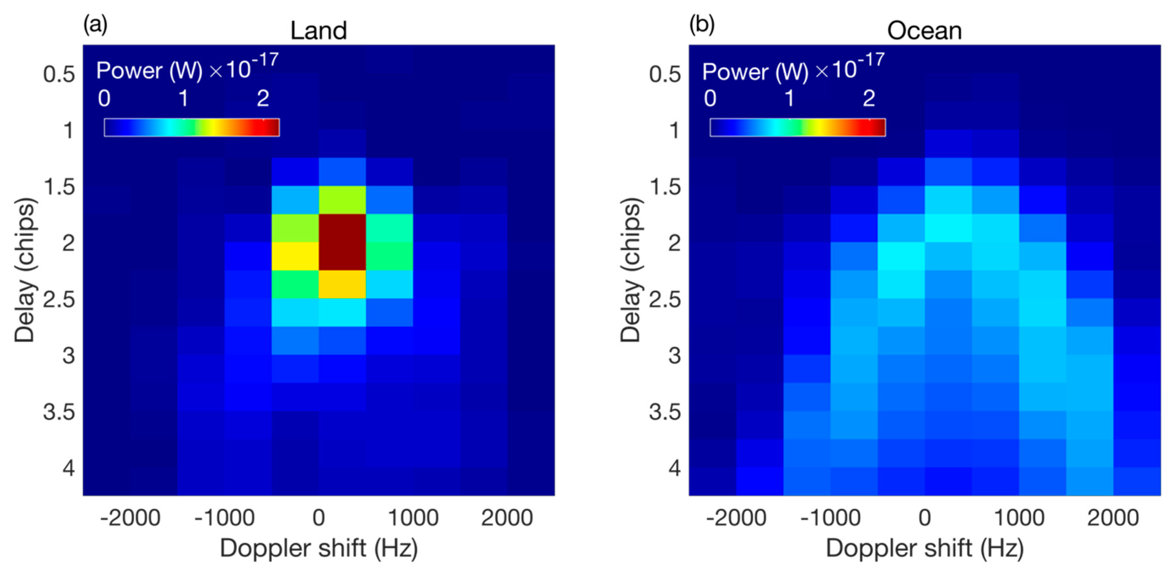
The reflected GNSS signal is recorded by the receiver in the form of what is called a delay-Doppler map (DDM). A DDM is created by cross-correlating the received signal with a locally generated replica that has been modified considering different path delays (resulting from the path distance between the transmitter, reflecting surface, and receiver, as shown in Figure 1) and Doppler shifts (resulting from the relative motions of the transmitter, reflecting surface, and the receiver). Two examples of DDMs are shown in Figure 3. Figure 3a is an example of a DDM recorded by CYGNSS over the land surface, and Figure 3b is an example of a DDM recorded over the ocean surface. The horseshoe shape of the ocean DDM is an indication that the reflection is incoherent and comes from a large, rough area. The absence of a horseshoe shape in Figure 3a indicates that the reflection is mostly coherent, and comes from a smaller, smoother area. The maximum power of each DDM is affected by surface roughness, the dielectric constant of the surface, and the vegetation overlying the surface, which is explained further below.
DDMs are most commonly used by summarizing them into one metric or observable. The observables that are commonly used for soil moisture estimation are the peak cross-correlation of each DDM or the peak divided by the noise floor (signal-to-noise ratio, SNR). The value of the peak cross-correlation of each DDM is related to surface characteristics at the specular reflection point of the GNSS signal, including the roughness of the surface, the surface dielectric constant, and properties related to any overlying vegetation such as vegetation water content and structure of the canopy. However, the peak of each DDM is also affected by variables unrelated to the reflecting surface, such as antenna gain and range. We describe our procedure to correct for these effects in the next section.
2. Materials and Methods
2.1. Introduction to the Algorithm
The algorithm presented here uses collocated soil moisture retrievals from the Soil Moisture Active Passive (SMAP) mission to calibrate concurrent (same calendar day) CYGNSS observations throughout a calibration period [44]. For a given location, a linear relationship between SMAP soil moisture and CYGNSS surface reflectivity observations is determined, and the relationship is used to transform all CYGNSS observations into soil moisture, even at times when there are no corresponding SMAP data points. Once the calibration is performed, it is applied to data outside the calibration period such that SMAP data are no longer required for ongoing CYGNSS soil moisture retrievals.
Using SMAP data for calibration of course comes with many drawbacks, the major one being that SMAP soil moisture retrievals are not soil moisture observations and have their own error and uncertainties. One must be careful when using CYGNSS data in areas where it is known that SMAP performs poorly. In addition, SMAP’s 40 km spatial resolution is likely coarser than that of CYGNSS. Intelligent upscaling of CYGNSS data to the 36-km EASE-2 grid that SMAP uses is necessary. If the resolution of CYGNSS is smaller than 36 km, then this effectively degrades the CYGNSS data and does not utilize it to its full potential. Despite the drawbacks associated with calibrating CYGNSS data with SMAP retrievals, SMAP data are considered to be one of, if not the, most accurate of the existing soil moisture products [45,46].
2.2. Algorithm Description
2.2.1. Derivation of Pr,eff
The first step in the retrieval algorithm is to calculate the effective surface reflectivity, which is the peak value of each delay-Doppler map (DDM) corrected for gain, range, and incidence angle effects. We call the uncorrected peak value of each DDM Pr.
Pr is affected by surface characteristics, such as the dielectric constant, roughness, and vegetation, as well as the gain of the receiving antenna, the bistatic range, and the power transmitted by each GPS satellite. We correct Pr for antenna gain, range, and GPS transmit power assuming a coherent reflection:
where is the transmitted RHCP power, is the gain of the transmitting antenna, is the distance between the transmitter and the specular reflection point, is the distance between the specular reflection point and the receiver, is the gain of the receiving antenna, is the GPS wavelength (0.19 m), and is the effective surface reflectivity.
We then solve for , which is the term affected by the surface roughness, dielectric constant of the soil, and vegetation by first converting all terms to dB:
Incidence angle is also expected to affect a coherent reflection, though this effect is only significant when the incidence angle is above 40 or 50 degrees. We correct for incidence angle in a similar way as in [29] by modelling how the effective surface reflectivity should change as a function of incidence angle, using established relationships (e.g., [47]). We call observations that have been corrected for incidence angle “Pr,eff,” which stands for the effective surface reflectivity.
2.2.2. Outlier Identification
Because CYGNSS was not optimized for remote sensing of the land surface, we remove observations that are flagged with standard quality measures as well as use empirical quality control that we have found to increase the effectiveness of our algorithm. Standard quality flags that we use are the following: “S-band transmitter powered up,” “spacecraft attitude error,” “black body DDM,” “DDM is a test pattern,” “direct signal in DDM,” and “low confidence in the GPS EIRP estimate.” Although it has been recommended that observations from the GPS Block IIF satellites be removed due to larger variations in GPS transmit power and consequently larger uncertainties in Pr [48], we keep these observations, as removing them reduces data volume by more than 30%.
Any data recorded before December 2017 reflecting from surface elevations greater than 600 m are removed. Prior to this time, the satellites did not record DDMs that contained the full surface reflection coming from these elevations.
We perform additional quality control measures that are not standardized in the analysis of CYGNSS data over oceans. These measures were developed after a detailed examination of outliers in regions where the surface is relatively constant over time (e.g., deserts). We remove any observation where Pr is less than 2 dB above the noise floor (SNR < 2 dB). We remove observations with a receiver antenna gain less than 0 dB, observations with an incidence angle greater than 65 degrees, any data with Pr occurring in a delay bin outside of 7–10 pixels (exclusive), and any observations that do not have a SNR less than or equal to the receiver antenna gain plus 14 dB.
2.2.3. Removal of Open Water Observations
The removal of specular reflection points that are affected by open water is a critical step before retrieving soil moisture. Even small water bodies ~25 m wide can significantly affect Pr,eff (e.g., Figure 1 from [28]). Our algorithm uses the Global Surface Water Explorer (GSWE) dataset described in [49], which is a 30-m water mask derived from Landsat data. Because it is derived from optical data, it cannot sense water beneath vegetation, though the L-band CYGNSS data is likely sensitive to some amount of water underneath a vegetation canopy. Additionally, because the GSWE is quasi-static in that it describes open water occurrence or when water occurs seasonally, it is not concurrent with the CYGNSS observations. The open water masking effort is thus imperfect, though we have found that it successfully removes a large amount of CYGNSS observations that are affected by open water.
The current algorithm removes open water using the “seasonality” data product provided by the GSWE. This product indicates how many months out of a year a pixel is inundated (0–12). For our purposes, we make this product binary by considering any value greater than 1 to be flagged as open water, and anything below this not to be open water. This is done because occasionally permanent water bodies are seasonally covered by vegetation, which makes the GSWE represent them as less than 12 (permanent). For each specular reflection point, we find the amount of water within a 7 × 7 km region surrounding the point. This is a simplification of the actual footprint, but it is computationally more efficient than rotating axes to form actual ellipses, which themselves are simplifications and not well quantified. If the amount of water in the 7 × 7 km region exceeds 1%, we remove that CYGNSS observation from consideration. Changing these thresholds or the size of the 7 × 7 km region does change the results, though never uniformly increasing or decreasing error across regions. It is possible that future versions of the soil moisture product will use a different open water masking procedure or incorporate CYGNSS coherence detectors, such as that described in [37], to aid in the detection of small water bodies.
2.2.4. Conversion of Pr,eff to Soil Moisture
We now describe how Pr,eff is transformed into soil moisture, using SMAP soil moisture retrievals to calibrate CYGNSS observations. Our calibration period was chosen to be 17 March 2017–1 October 2018. This is an extended period beyond what was shown in [28]. In our calibration, we use all SMAP retrievals regardless of SMAP quality flags to allow for the retrieval of soil moisture from CYGNSS for the entirety of CYGNSS’ observational area. Of course, users should be cautious to use CYGNSS soil moisture retrievals from regions regularly flagged by SMAP, such as the dense forests of South America and Africa, which are indicated in the CYGNSS quality flags.
The algorithm is based on the assumption that Pr,eff is linearly related to SMAP soil moisture. The linear relationship is allowed to vary spatially, but we assume that it does not change over time. For a given location, we calculate the slope of the best-fit linear regression between concurrent (same calendar day) SMAP soil moisture retrievals and CYGNSS Pr,eff, after having removed the mean of each for the entire time series. Before we can describe this in more detail, however, we must explain what “a given location” means in this context.
In Section 1.2, we described how the smallest theoretical (no roughness) spatial footprint of CYGNSS over land is approximately 7 × 0.5 km, or 3.5 × 0.5 km for data recorded after mid-2019. What the actual spatial resolution is over land is a matter of debate within the GNSS-R community, though our own analysis of how Pr,eff varies with small landcover or topographic features indicates to us that the effective footprint is likely only a few km, much smaller than SMAP’s 40 km resolution [28]. If, for every SMAP observation, the CYGNSS observations completely sampled the 36-km EASE-2 grid cell used by SMAP, then a simple averaging could be used to aggregate CYGNSS observations to match with the SMAP retrieval. However, this is not the case. For every SMAP observation, there will likely be several CYGNSS observations within the grid cell, though not enough to completely sample the grid cell, if the spatial footprint is small (< 10 km). In this case, simple averaging will lead to variations in the day-to-day signal due to differential sampling of landcover types and topography within the SMAP pixel, which could be mistaken for variations in soil moisture.
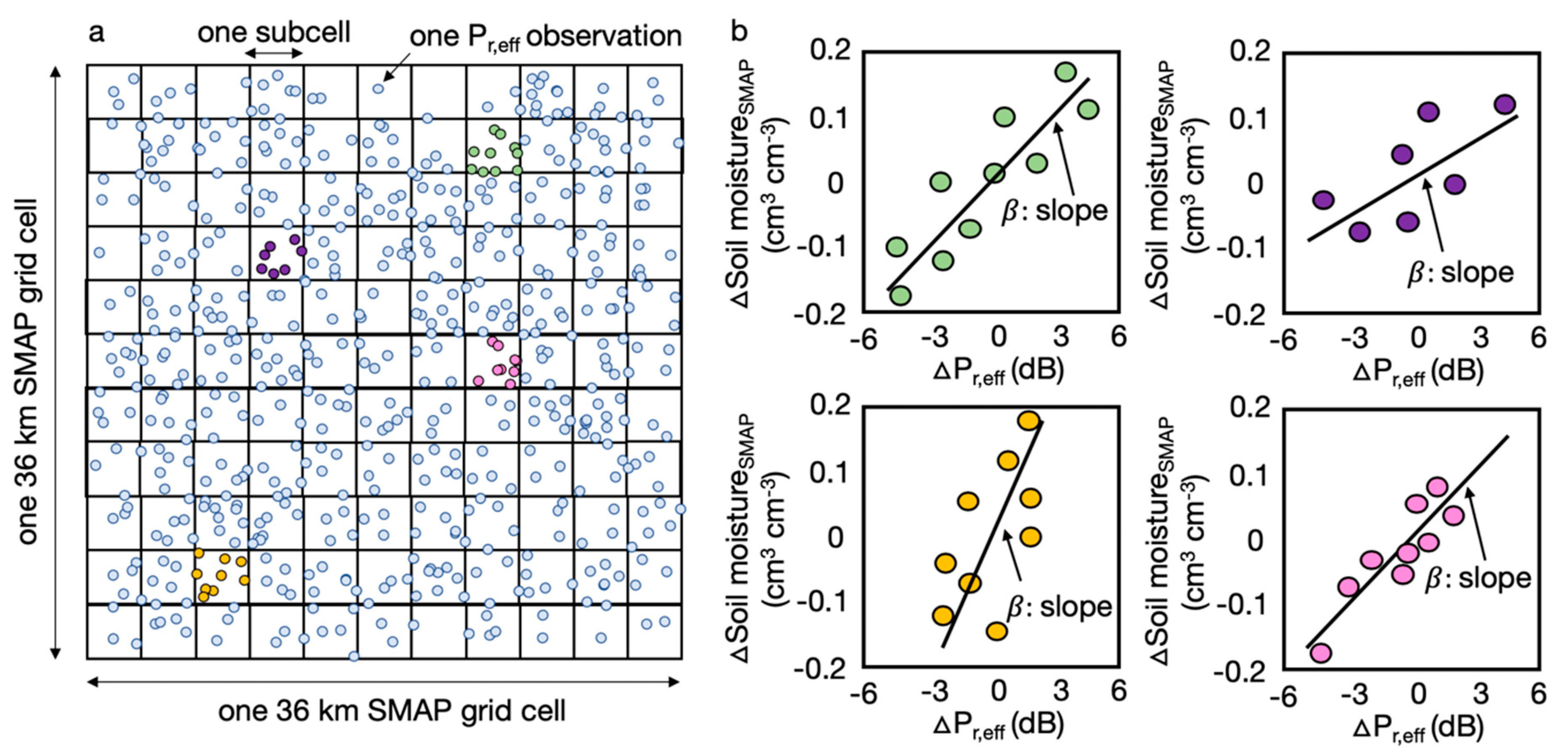
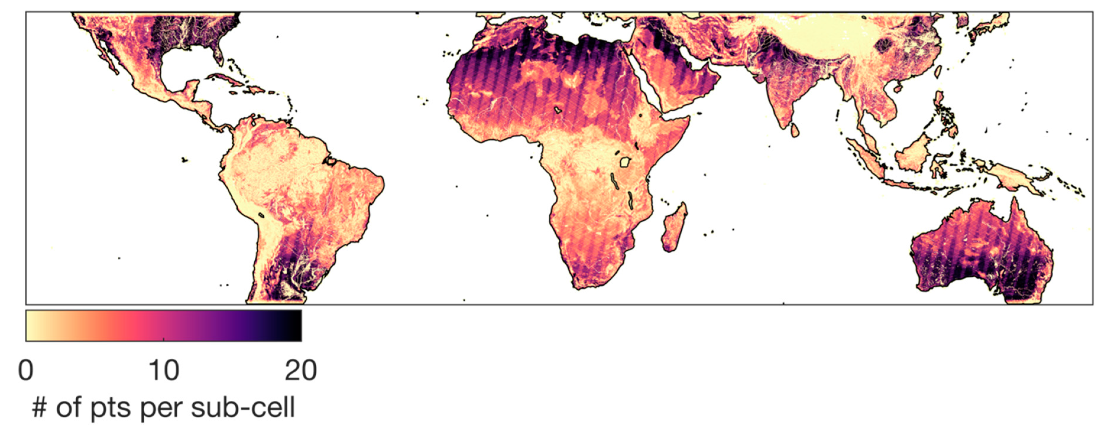
In order to avoid this, we first grid our Pr,eff observations to ~3 × 3 km “subcells,” retrieve soil moisture from the subcells, and then aggregate the gridded observations to the 36-km SMAP EASE-2 grid resolution (Figure 4a). This subcell approach minimizes the confounding effects of landcover and topography on Pr,eff. The number of points per subcell in the calibration period are shown in Figure 5—subcells with less than three observations were not used for calibration.
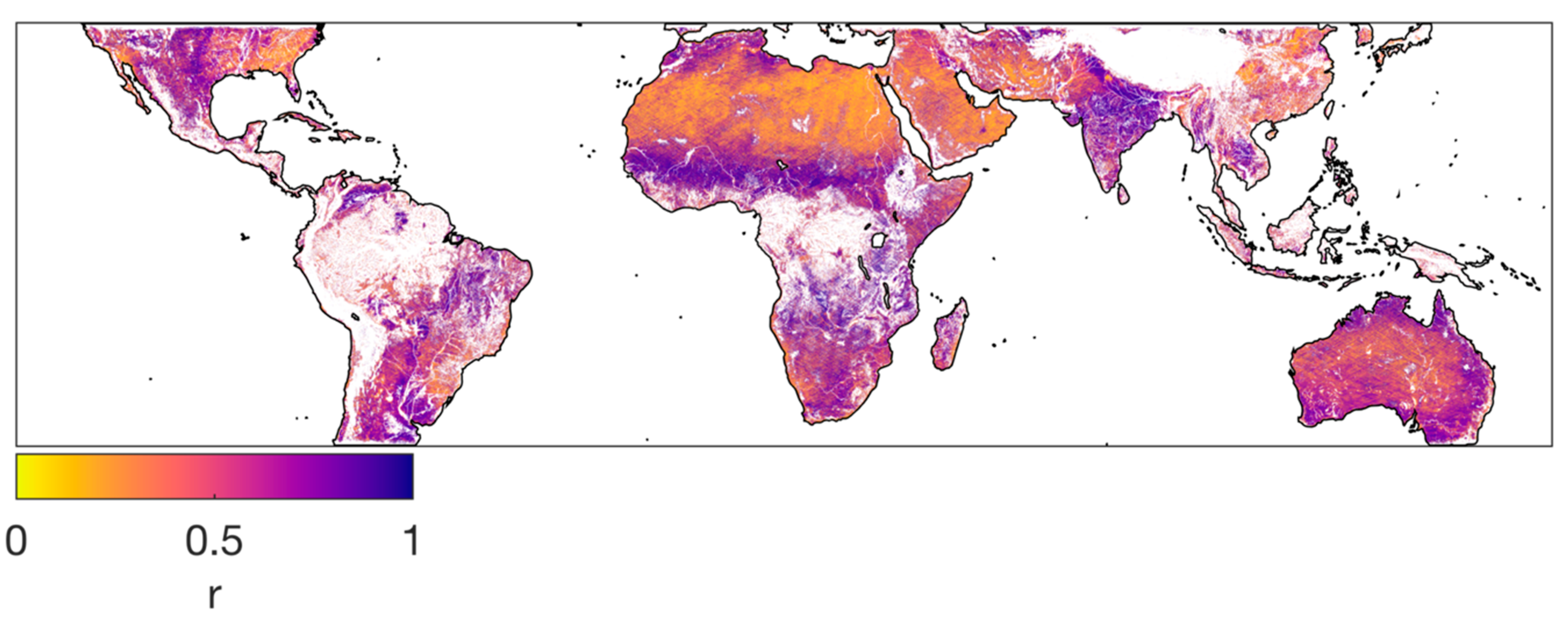
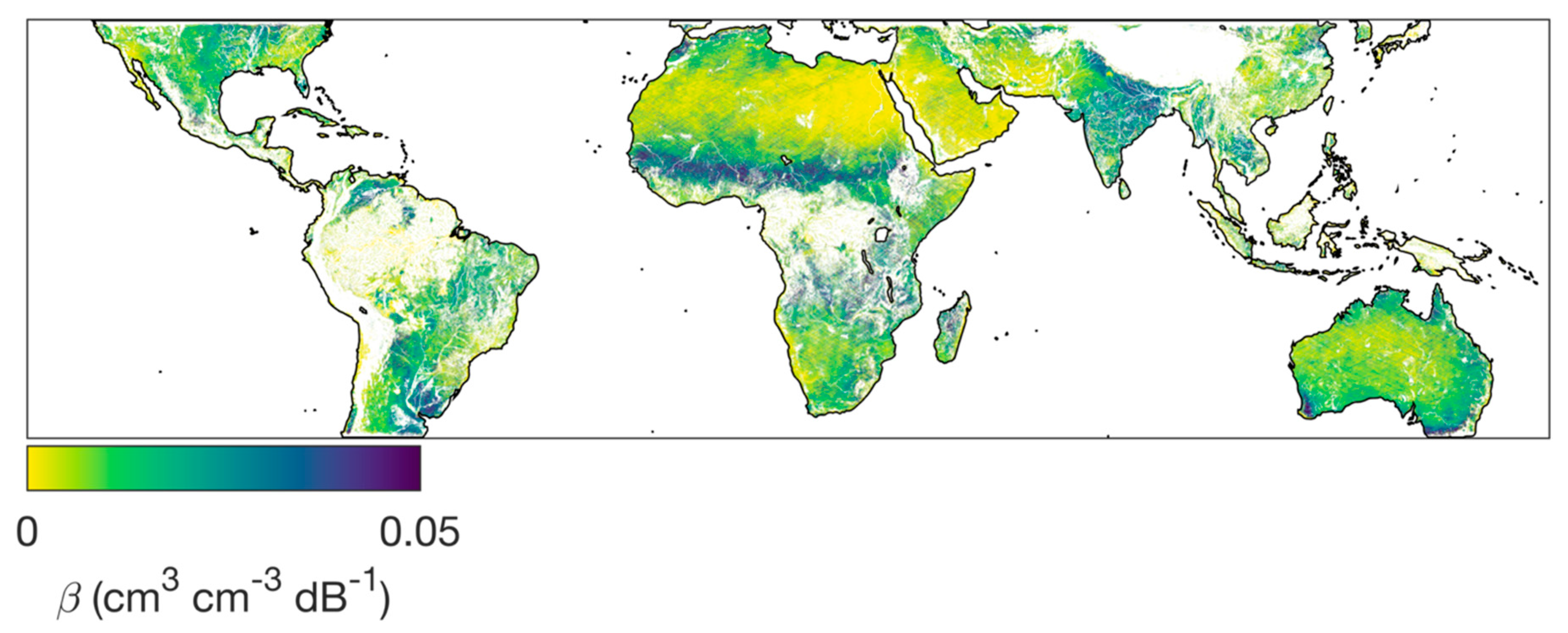
Within each subcell, we calculate the linear regression between SMAP soil moisture and Pr,eff match-ups (occurring on the same calendar day), after having removed the mean values of both SMAP soil moisture and Pr,eff in that subcell. The slope of the linear regression is , which is conceptualized in Figure 4b. The correlation coefficients for these relationships are shown in Figure 6. varies spatially (Figure 7). Some of the spatial variability is likely real, and it could be the result of spatial variations in topography or landcover. Some of it, however, is likely the result of the fact that some arid regions do not have enough soil moisture variability throughout the year in order to adequately calculate . In these regions, is artificially low because any noise in the CYGNSS observations will significantly affect the linear regression [28].
is then used to estimate soil moisture from CYGNSS for data falling outside the calibration period as well as data within the calibration period when there are no SMAP match-ups (since SMAP has a 2–3 day overpass period) using the following equation:
where is the soil moisture derived from one CYGNSS observation at time, t, is one observation of at time, t, is the mean value of for a particular subcell during the calibration period, and is the mean SMAP soil moisture during the calibration period. The mean values of both SMAP and CYGNSS during the calibration period serve as our reference values, in order to return an absolute value of soil moisture from CYGNSS. Once retrievals are made for individual subcells, the mean of the retrievals for all subcells within each 36-km grid cell is used as the final CYGNSS soil moisture retrieval. Note that not all subcells within one 36-km grid cell will be sampled for each time step, and there could be times when just one subcell is used for the retrieval. The timesteps at which retrievals are averaged is described below.
2.2.5. Daily and Sub-Daily Retrievals
Soil moisture retrievals are currently provided on daily and sub-daily (6 hourly) time steps. For the daily retrievals, we average all CYGNSS soil moisture retrievals within a particular 36-km grid cell that fall within the 24-hour time period. For the sub-daily retrievals, we average all retrievals for a grid cell in 6-hour intervals, which are currently midnight–6 am, 6 am–noon, noon–6 pm, and 6 pm–midnight (UTC). Note that, just because retrievals are provided at 6-hour time steps, it does not mean that there will be values everywhere at every time step. There will be missing values in some grid cells even when aggregated to a 24-hour time step.
2.2.6. Quality Control
There is currently only minimal quality control of the soil moisture retrievals themselves. Soil moisture retrievals that are either less than 0.01 cm3 cm−3 or greater than 0.65 cm3 cm−3 are removed, though users should apply their own additional thresholds when using retrievals in specific regions that may have higher or lower residual or saturated moisture contents.
2.2.7. Soil Moisture Retrieval Uncertainty
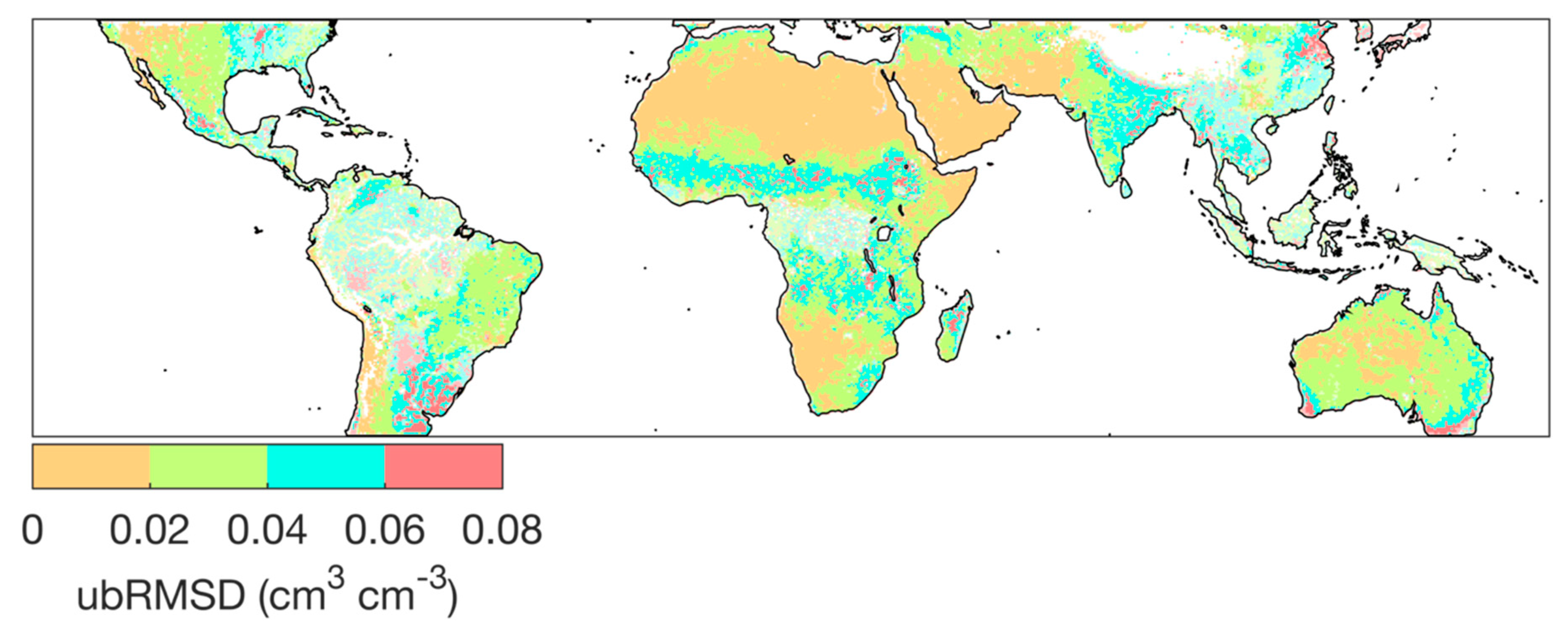
Figure 8 shows the unbiased root-mean-square difference (ubRMSD) between CYGNSS and SMAP soil moisture retrievals for the calibration period (18 March 2017–1 October 2018). Semi-transparent regions are those frequently flagged by SMAP as being poor quality. Higher values of ubRMSD tend to cluster in areas that flood seasonally, which indicates imperfect open water masking, or have greater soil moisture variability throughout the year. It is “easier” to have a lower ubRMSD in regions with lower soil moisture variability.
2.2.8. Quality Flags
Static quality flags are provided in a separate file from the soil moisture retrievals. Examining the quality flags is a crucial first step before using the CYGNSS soil moisture retrievals or interpreting the empirical sensitivity of CYGNSS to soil moisture (). The flags were developed to encourage users to exercise caution when using soil moisture from certain regions, or to be careful in the interpretation of from these regions. The following criteria were used in the development of the flags:
- Regions where CYGNSS observations were calibrated to SMAP data where a large portion (>90%) of the SMAP soil moisture retrievals were flagged as “not recommended for retrieval.” These data tend to be in regions that are forested, with significant topography, or near coastlines. Although the overall ubRMSE between CYGNSS retrievals and in-situ observations remains largely unchanged for sites located in these regions, there are fewer instances where the ubRMSE is < 0.04 cm3 cm−3.
- Regions where CYGNSS was calibrated to SMAP data with a small range of soil moisture values (<0.1 cm3 cm−3). This indicates a larger uncertainty in [28]. The ubRMSE between CYGNSS and in-situ observations in these regions is low (0.0395 cm3 cm−3) due to the fact that there is only small variability in soil moisture. In these regions, because there is a larger uncertainty in , we do not want users to make any interpretations about , or attempt to compare it to modelled sensitivity.
- Regions where the ubRMSD between CYGNSS and SMAP was large for the calibration period (> 0.08 cm3 cm−3). The ubRMSE between CYGNSS and in-situ stations with this condition was higher than average (0.0561 cm3 cm−3). Users are advised to use caution when analysing retrievals from these areas. In-situ stations used for validation are described in the next section.
- Regions with few observations in the 36 km grid cell for calibration, leading to less certain retrievals outside the calibration period (n < 100). is also more uncertain in these regions.
- Regions where is low (<5 dB). There is a higher likelihood that roughness or vegetation effects dominate in these areas. Soil moisture retrievals from these areas are particularly suspect—the ubRMSE between CYGNSS and in-situ observations located in these regions is 0.07 cm3 cm−3. We advise users against using CYGNSS soil moisture retrievals at these locations.
3. Results
We validated the UCAR/CU CYGNSS Soil Moisture Product at 171 in-situ soil moisture sites from six different networks: COSMOS [50], PBOH2O [51], SCAN [52], SNOTEL [53], USCRN [54], and OzNet [55]. The time period chosen for validation was 2 October 2018–31 December 2019, so as to not overlap with the calibration period. However, not all stations had data for the entire validation time period. In particular, sites within the PBOH2O network (a ground-based GNSS reflectometry network) only contained data through the first six weeks of the validation time period. Note that the majority of the validation sites are located in the United States—just because there may be acceptable agreement between CYGNSS and in-situ observations at these locations, it does not mean that CYGNSS is expected to perform as well in environments extremely disparate from those typical of the United States (e.g., tropical rainforests). Before validation, we removed obviously non-sensical soil moisture data from the in-situ records, for example soil moisture observations below 0 cm3 cm−3 or greater than 1 cm3 cm−3.
We calculated the median unbiased root-mean-square error (ubRMSE) between daily averaged CYGNSS retrievals and in-situ observations for each individual station (Table A1) as well as aggregated by network (Table 1). Note that here we use ubRMSE, whereas before we used ubRMSD to compare SMAP and CYGNSS retrievals. Though we calculated them the same way, we use ubRMSE here to indicate that this is a validation exercise, whereas the comparison between SMAP and CYGNSS was only for the purpose of showing where the two products are dissimilar from one another. For context, we also calculated the ubRMSE between SMAP retrievals and in-situ observations for the same time period. These values are also contained in Table 1 and Table A1. Overall, the median ubRMSE between CYGNSS and in situ (0.049 cm3 cm−3) and SMAP and in situ (0.045 cm3 cm−3) were very similar, given that the standard deviations of each were ~0.025 cm3 cm−3. Similar ubRMSEs are expected since that CYGNSS was calibrated from SMAP retrievals.
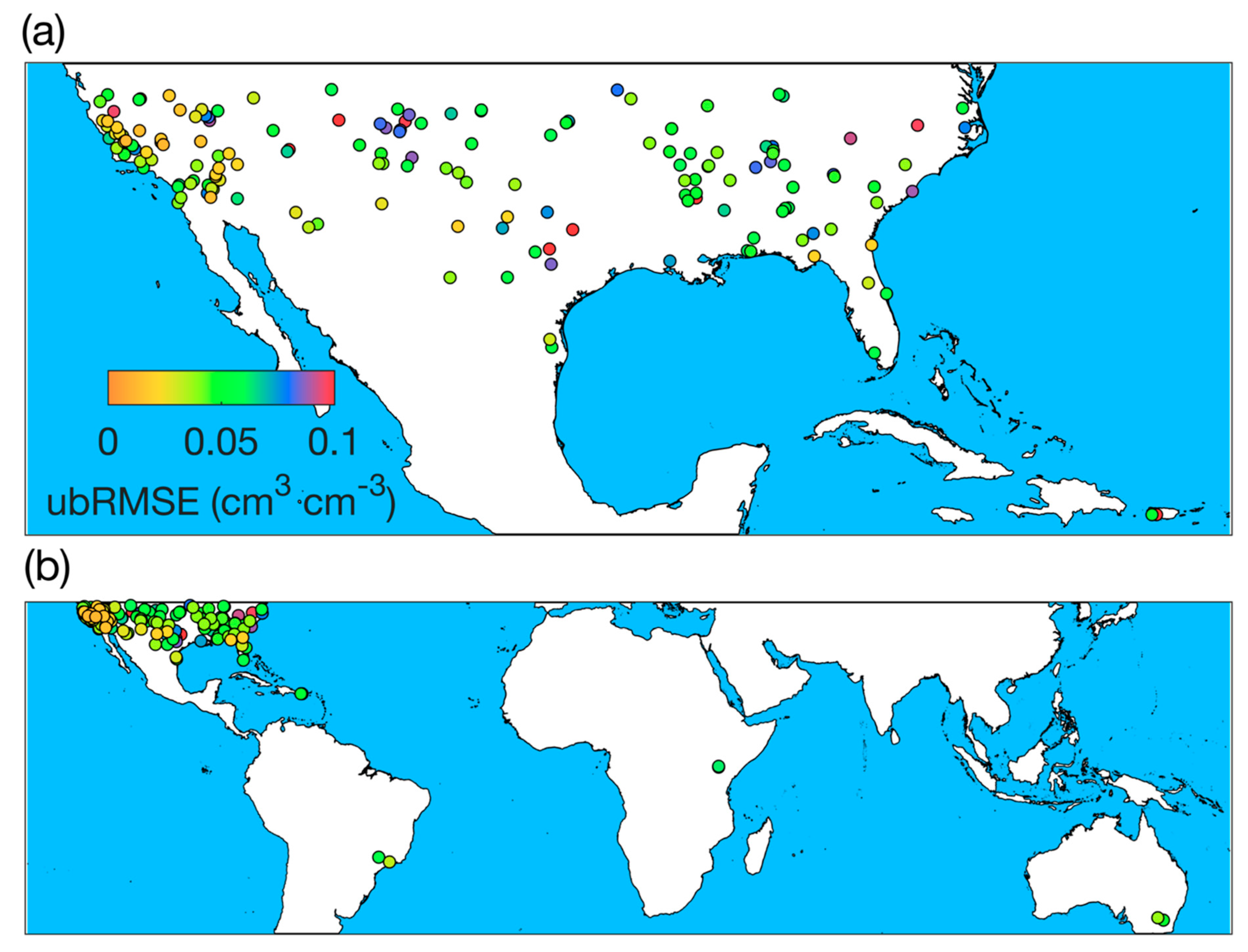
A map of all in-situ stations used in this validation exercise along with their respective ubRMSE values is shown in Figure 9. Note that there is a wide range of ubRMSE values, depending on the site and network. In particular, SNOTEL sites performed poorly (mean ubRMSE ~= 0.09 cm3 cm−3). SNOTEL sites tend to be in mountainous areas with surrounding trees. in these regions tends to be low, which is an indicator that either topographic roughness or dense vegetation is significantly affecting the reflected signal. We caution users who are interested in using the CYGNSS retrievals in such areas, given the high validation ubRMSE at the in-situ sites. The quality flags described in the last section delineate where these effects are likely to be at play.
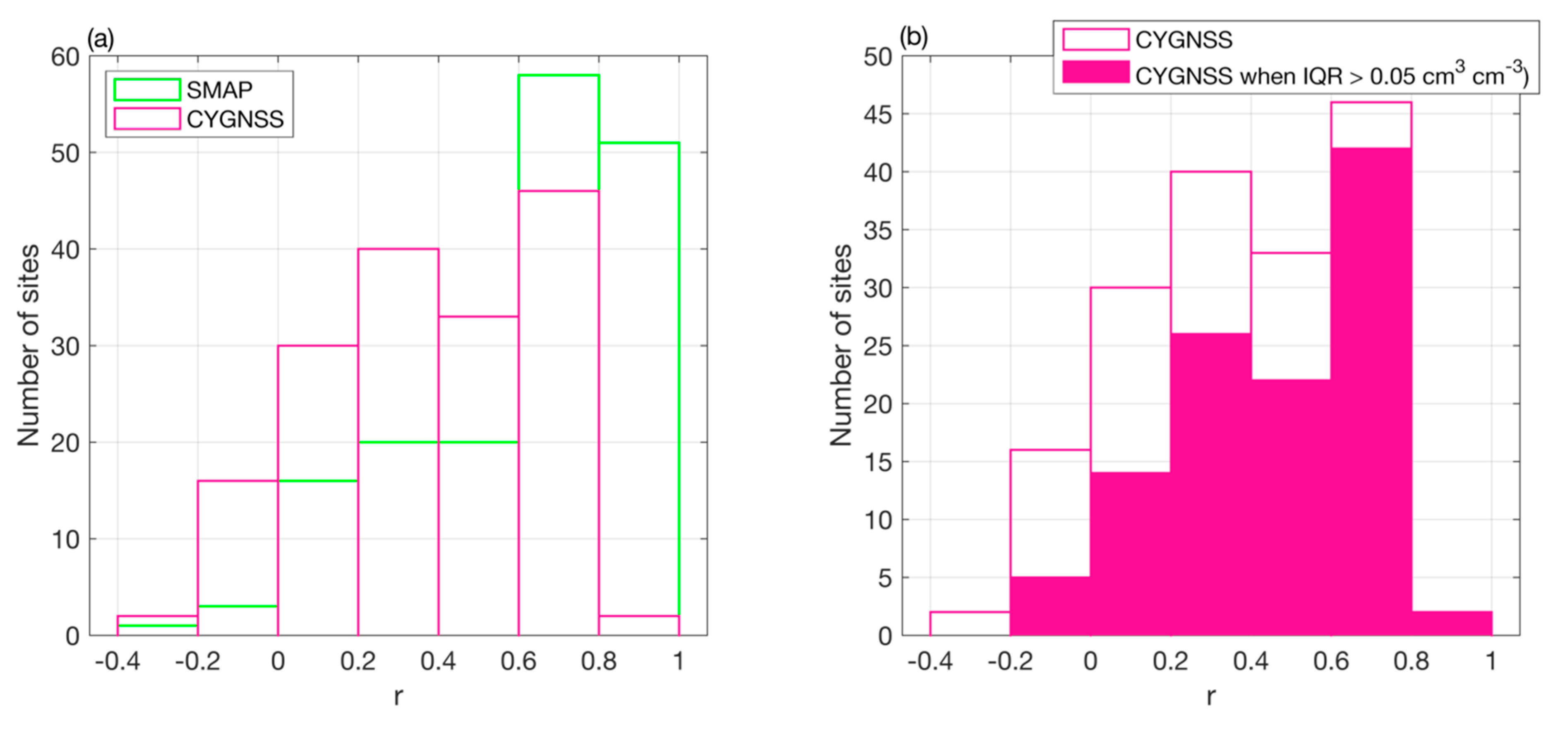
Table A1 also includes other validation metrics, such as the correlation coefficient (r) between CYGNSS and in-situ sites and the mean bias between in-situ observations and SMAP retrievals, which by extension is also the bias between in-situ observations and CYGNSS retrievals. The median correlation coefficient across sites is somewhat low (r = 0.4) but with a large standard deviation (0.27). Figure 10a shows a histogram of the correlation coefficient (r) between CYGNSS and in-situ observations, with that from SMAP shown for context. Compared to SMAP, CYGNSS has a wider distribution of correlation coefficients, with a lower median value (Table 1). Similar to what was discussed in relation to the correlation between CYGNSS effective reflectivity and SMAP soil moisture, areas with low or no soil moisture variation during the validation time period often results in a low correlation coefficient, as any effects due to random noise are amplified when there is no soil moisture variation. CYGNSS retrievals are expected to have more noise than SMAP retrievals, given the aforementioned imperfections in signal calibration and lack of full grid cell coverage. Figure 10b shows that the distribution of r values does change significantly when only in-situ sites with moderate or large soil moisture variability are considered, which helps mask the effect of noise. In addition to the correlation coefficient, the median absolute bias between SMAP and in-situ observations, which will also be the bias between CYGNSS and in-situ, is 0.05 cm3 cm−3. This dry bias is a known issue in the SMAP retrievals [56].
Validating a satellite remote-sensing product based off of point measurements, as we have done here, is an imperfect exercise, as the individual soil moisture probe observations may not be representative of the larger areal average. The validation effort conducted by SMAP, for example, averaged in-situ observations from many probes spread out over a large area, for each of their validation sites [46]. The sites that comprise OzNet do indeed contain multiple probes at each site, though there are only two sites with data within the calibration time period (see Table A1). In this case, we used the mean of all probe measurements within one site to calculate the ubRMSE. CYGNSS soil moisture retrievals did agree better with the in-situ observations from these sites (ubRMSE = 0.043 cm3 cm−3) than they did from the point-based observations.
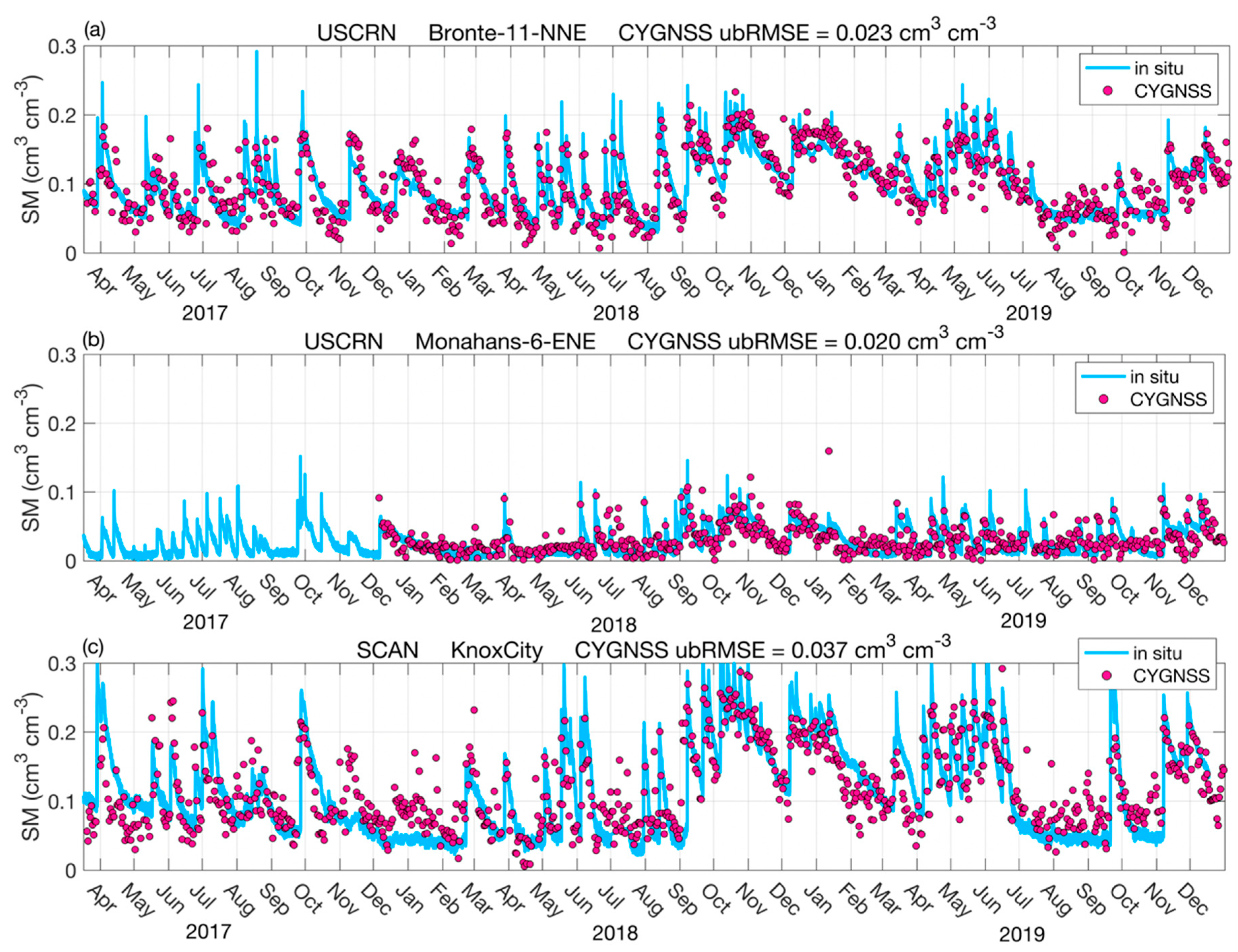
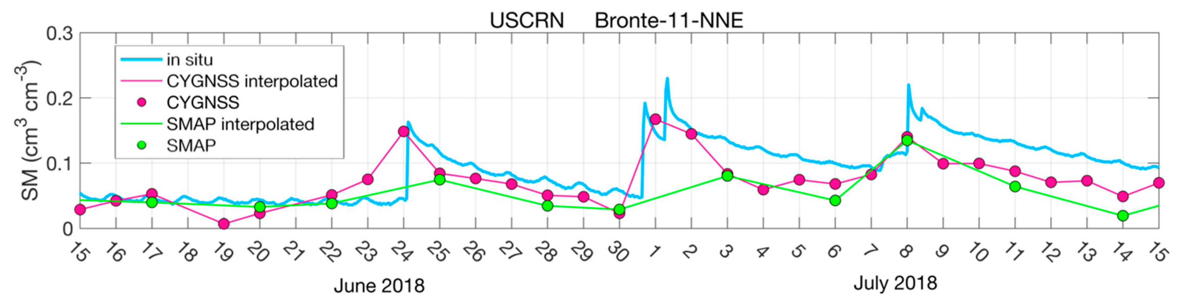
Examples of CYGNSS soil moisture time series that agree well with in-situ observations are shown in Figure 11. These sites show that CYGNSS has the ability to retrieve both low and high soil moisture contents. An example of the increased temporal resolution of daily averaged CYGNSS retrievals with respect to SMAP is shown in Figure 12. In this example, the increased resolution of CYGNSS results in the observation of increased soil moisture due to two precipitation events in late June and early July of 2018, which are missed by SMAP. Table A1 shows how many daily averaged CYGNSS soil moisture retrievals were available during the validation time period, which can be compared to the number of SMAP retrievals for the same time period. On average CYGNSS soil moisture retrievals increase the temporal revisit time by 63.4%.
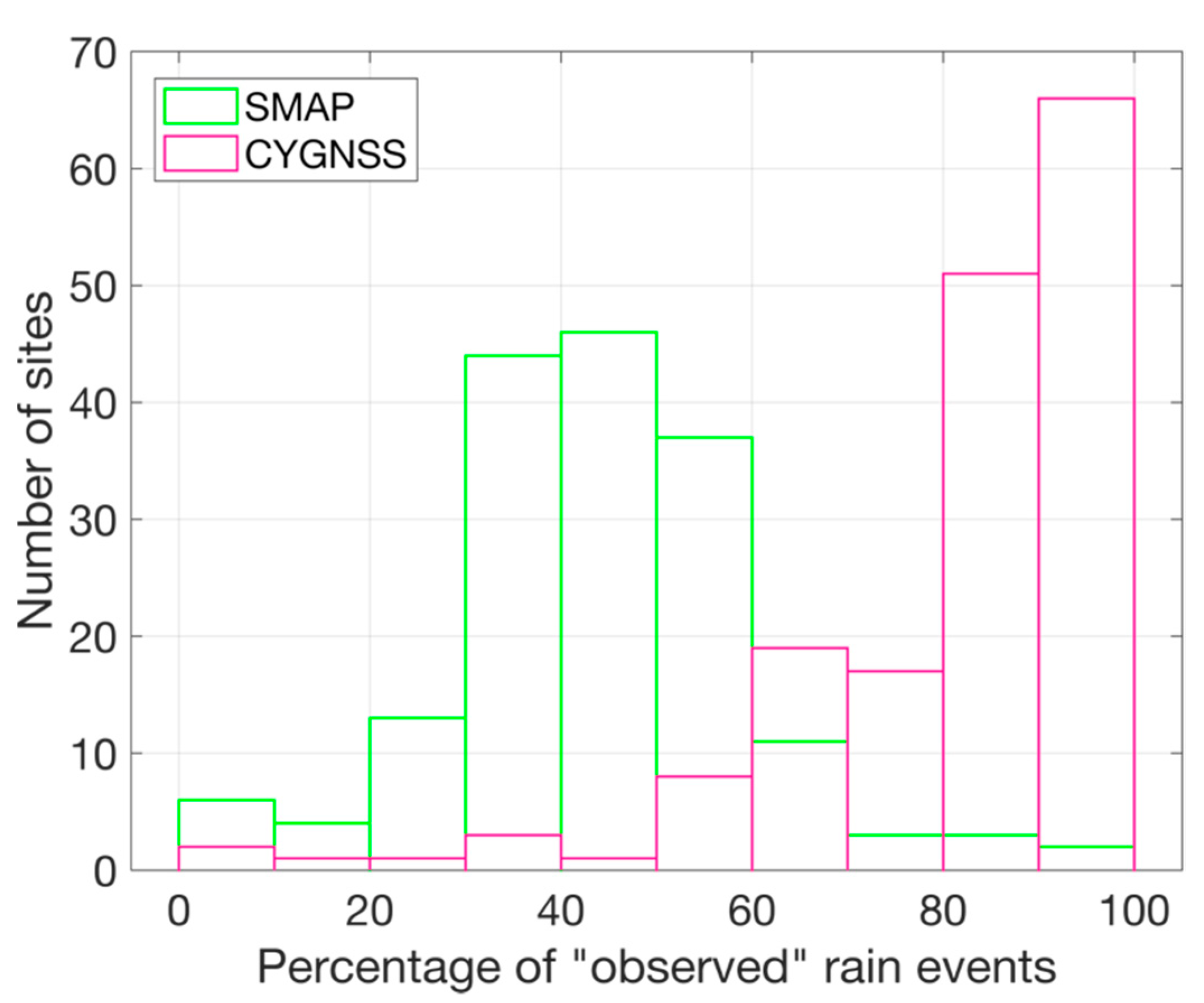
For each in-situ site, we calculated the number of rain events during the validation period, which we defined as an increase in the daily averaged soil moisture greater than 0.02 cm3 cm−3. We then calculated the number of the rainy days that had CYGNSS observations and the number that had SMAP observations. From this, we could calculate the percentage of rain events “observed” by both CYGNSS and SMAP and found that CYGNSS observed a median of 87% of the rain events, and SMAP observed a median of 43% (distributions shown in Figure 13). At sites with acceptable CYGNSS performance, CYGNSS would be able to provide more information about soil drying and wetting than SMAP currently is able to.
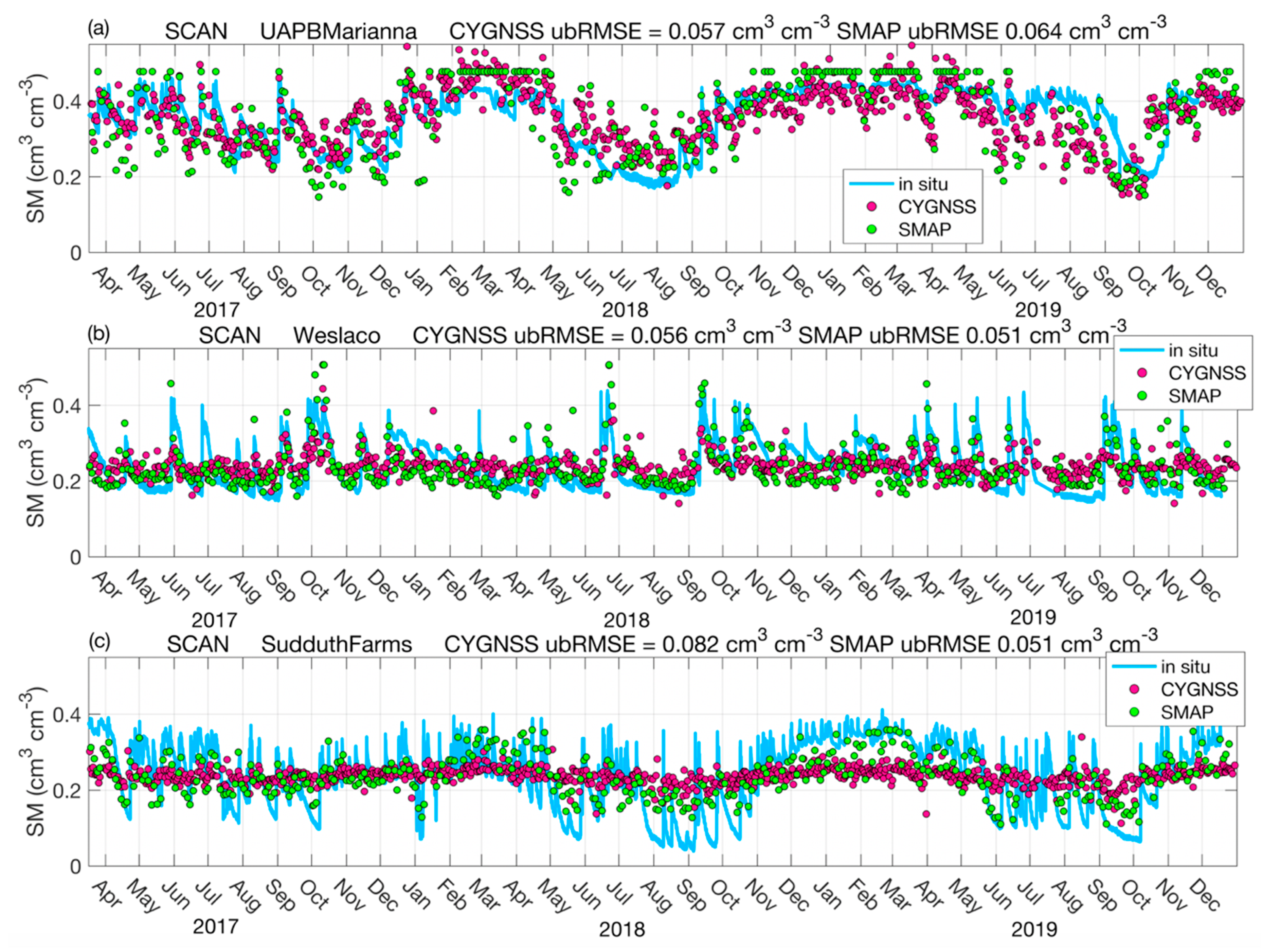
Figure 14 shows three examples of soil moisture time series from CYGNSS and SMAP where CYGNSS does not agree well with in-situ observations. Generally, if SMAP does not perform well at a site, CYGNSS is likely to perform poorly, too. However, there are other sites where SMAP performance is significantly more acceptable than that from CYGNSS (e.g., Figure 14c). Understanding why CYGNSS soil moisture retrievals at some locations do not perform as well as SMAP is one subject of future research, though preliminary analyses indicate that inadequate open water masking could be one contributing factor.
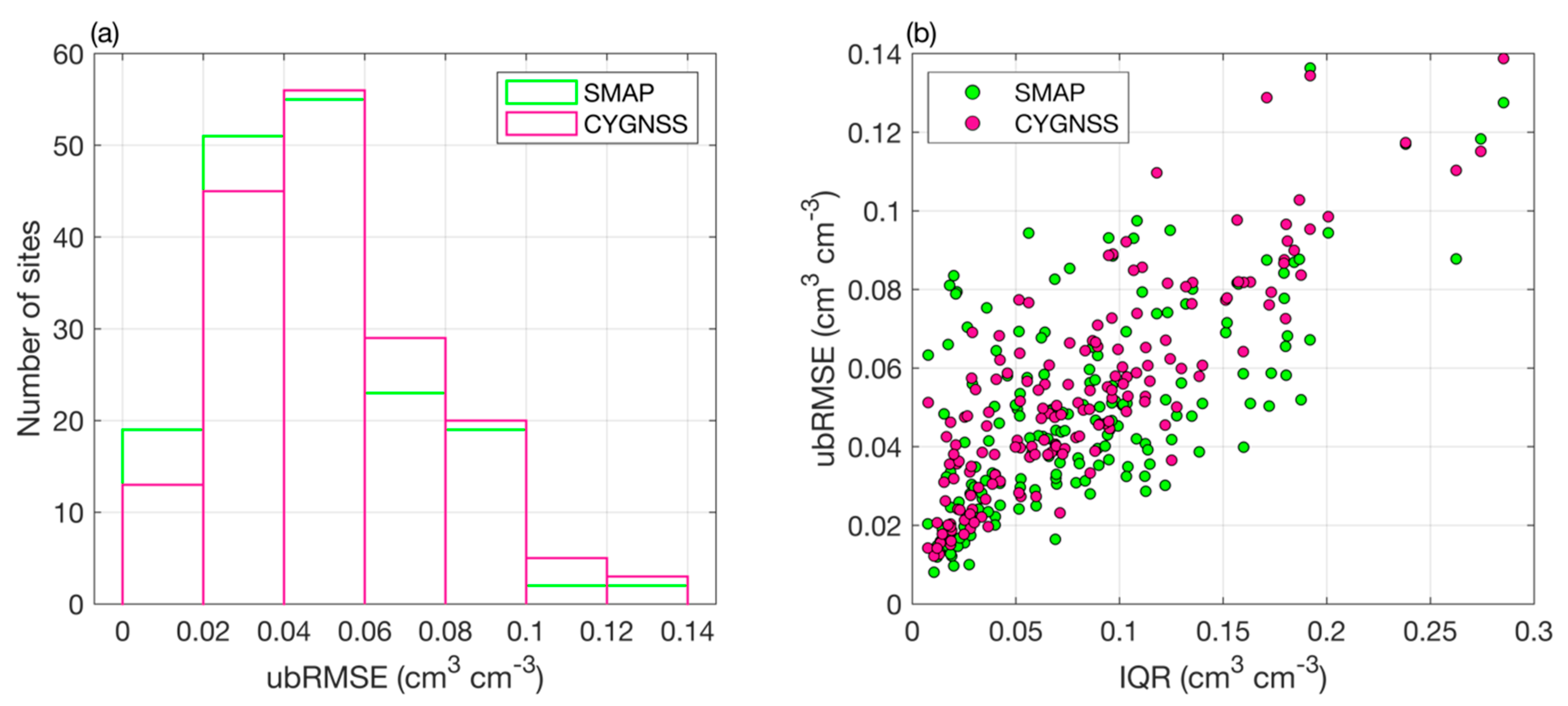
Figure 15a shows a histogram of the ubRMSEs between CYGNSS and in-situ observations (values in Table A1), with that from SMAP shown for context. Although the median ubRMSE for both CYGNSS and SMAP retrievals are lower than 0.05 cm3 cm−3, it is important to note that ubRMSE statistics are correlated with the variability of soil moisture at a particular site. Figure 15b shows the ubRMSE of CYGNSS and SMAP as a function of the interquartile range (IQR) of soil moisture for each site. As soil moisture variability increases, so does the ubRMSE. This means it may be unreasonable to assume an error of 0.04 cm3 cm−3 in areas that undergo extreme fluctuations in soil moisture throughout the year. For context, the median IQR at validation sites was 0.07 cm3 cm−3, and the IQR of USCRN station Bronte-11-NNE shown in Figure 11 and Figure 12 is 0.071 cm3 cm−3.
4. Discussion
As with all remote-sensing techniques, there are limitations to what information retrieval algorithms can provide. Below are some of the more significant limitations of the UCAR/CU retrieval algorithm. We avoid commenting on limitations of CYGNSS in general and instead only address the specific algorithm presented here.
- Errors in SMAP retrievals will propagate into CYGNSS soil moisture retrievals. Because CYGNSS is calibrated using SMAP, any systemic errors in the SMAP retrievals (particularly, persistent bias) will also be present in CYGNSS retrievals. As discussed above, at validation sites with poor SMAP performance, CYGNSS also performs poorly.
- As with all empirical approaches, investigation into the “true” sensitivity to soil moisture is difficult. As mentioned above, unless there is enough soil moisture variability, calculation of is difficult due to noise in the CYGNSS observations. Additionally, if there is variability of within a subcell due to, for example, spatial variations in land cover, then may appear artificially high (i.e., low sensitivity to soil moisture).
- The relationship between and soil moisture may not actually be linear. Although we approximate the relationship as being linear, it may not be—it may appear to be linear either due to noise overwhelming an obvious non-linearity, or it may appear linear because in many regions soil moisture does not often fluctuate between 0.02 cm3 cm−3 and 0.5 cm3 cm−3 or higher, which would be necessary to elucidate significant non-linear relationships. The empirical linear relationships may thus not match those eventually derived from a model and should not be compared.
- The assumption that the sensitivity of to soil moisture does not change over time is likely incorrect. Fluctuations in vegetation water content, particularly in agricultural regions, will likely change , though we currently ignore that possibility.
- Aggregating CYGNSS observations to 36 km does not take advantage of the finer spatial resolution. Any advantages CYGNSS might have vis-à-vis providing higher spatial resolution soil moisture retrievals is not permitted by the approach that we use here. Other approaches using either machine learning methods or models could be successful, if provided with accurate, high-resolution ancillary data.
5. Conclusions
This paper described the UCAR/CU CYGNSS Soil Moisture Product [19], which uses spaceborne GNSS-R reflections, calibrated to SMAP soil moisture, to produce soil moisture retrievals. Validation of the product at 171 in-situ soil moisture stations resulted in a median ubRMSE of 0.049 cm3 cm−3. This product can be used by hydrologists who are interested in soil moisture data at a higher temporal resolution than currently available using other products. As was shown in Figure 12 and Figure 13, CYGNSS can observe changes in soil moisture due to precipitation events that may be too quick for the SMAP overpass period. The quantification of soil moisture memory, observation of moisture conditions giving rise to flooding, and the inverse estimation of precipitation using soil moisture time series all require soil moisture data on short time scales, and a daily soil moisture product may be able to provide more complete information on soil moisture dynamics at needed time scales.
GNSS-R researchers interested in developing independent CYGNSS soil moisture retrievals using model-based approaches may also benefit from using this product, as it can provide an indication of where simple algorithms like this one can successfully retrieve soil moisture and where more complicated approaches may be warranted.
Author Contributions
Conceptualization, C.C. and E.S.; methodology, C.C. and E.S.; software, C.C.; validation, C.C. and E.S.; writing, C.C. and E.S. All authors have read and agreed to the published version of the manuscript.
Funding
This research received no external funding.
Acknowledgments
We would like to thank Jan Weiss and Maggie Sleziak of UCAR for putting the soil moisture product online and the CYGNSS team for providing high quality GNSS-R data.
Conflicts of Interest
The authors declare no conflict of interest.
Appendix A

Table A1.
Location information and statistics for each in-situ soil moisture station used for validation. Unbiased root-mean-square errors (ubRMSEs) for CYGNSS are shown as well as those for SMAP, which are shown for context. The correlation coefficient (r) between CYGNSS soil moisture retrievals and in-situ observations is shown. The bias between SMAP retrievals and in-situ observations is the same as for CYGNSS retrievals and in-situ observations, since CYGNSS retrievals are already bias-corrected with respect to SMAP. The number of CYGNSS and SMAP observations used for calculation of ubRMSEs, r, and the bias are also shown.
| Network | Station | Latitude (deg) | Longitude (deg) | ubRMSE CYGNSS (cm3 cm−3) | ubRMSESMAP (cm3 cm−3) | r CYGNSS | Bias SMAP | # Obs CYGNSS | # Obs SMAP |
|---|---|---|---|---|---|---|---|---|---|
| COSMOS | COSMOS_064 | 35.19 | −102.10 | 0.054 | 0.056 | 0.61 | 0.16 | 182 | 91 |
| COSMOS | COSMOS_101 | −22.68 | −45.00 | 0.033 | 0.022 | 0.06 | −0.08 | 220 | 125 |
| COSMOS | COSMOS_023 | 33.61 | −116.45 | 0.051 | 0.037 | 0.17 | 0.01 | 289 | 167 |
| COSMOS | COSMOS_057 | 29.95 | −98.00 | 0.086 | 0.079 | 0.50 | 0.12 | 269 | 105 |
| COSMOS | COSMOS_067 | 34.26 | −89.87 | 0.042 | 0.050 | 0.50 | −0.19 | 301 | 164 |
| COSMOS | COSMOS_055 | 0.28 | 36.87 | 0.071 | 0.040 | 0.50 | 0.09 | 152 | 88 |
| COSMOS | COSMOS_050 | 0.49 | 36.87 | 0.062 | 0.031 | 0.50 | −0.10 | 113 | 60 |
| COSMOS | COSMOS_034 | 37.07 | −119.19 | 0.129 | 0.087 | 0.34 | −0.03 | 98 | 154 |
| COSMOS | COSMOS_044 | −21.62 | −47.63 | 0.057 | 0.030 | 0.04 | −0.18 | 90 | 57 |
| COSMOS | COSMOS_014 | 36.06 | −97.22 | 0.049 | 0.038 | 0.39 | −0.07 | 237 | 118 |
| COSMOS | COSMOS_033 | 37.03 | −119.26 | 0.053 | 0.041 | 0.31 | −0.07 | 21 | 12 |
| PBOH2O | bkap | 35.29 | −116.08 | 0.016 | 0.016 | 0.20 | 0.01 | 33 | 20 |
| PBOH2O | crrs | 33.07 | −115.74 | 0.077 | 0.069 | -0.01 | −0.10 | 36 | 14 |
| PBOH2O | csci | 34.17 | −119.04 | 0.052 | 0.054 | 0.05 | −0.04 | 33 | 14 |
| PBOH2O | ctdm | 34.52 | −118.61 | 0.034 | 0.023 | −0.14 | 0.09 | 26 | 14 |
| PBOH2O | fgst | 34.73 | −120.01 | 0.046 | 0.034 | 0.03 | 0.05 | 22 | 19 |
| PBOH2O | glrs | 33.27 | −115.52 | 0.032 | 0.084 | −0.04 | −0.18 | 35 | 15 |
| PBOH2O | gnps | 34.31 | −114.19 | 0.022 | 0.010 | 0.38 | −0.02 | 35 | 19 |
| PBOH2O | hunt | 35.88 | −120.40 | 0.020 | 0.013 | 0.33 | −0.02 | 22 | 19 |
| PBOH2O | hvys | 34.44 | −119.19 | 0.036 | 0.079 | 0.00 | −0.30 | 34 | 19 |
| PBOH2O | imps | 34.16 | −115.15 | 0.019 | 0.021 | 0.51 | 0.04 | 34 | 19 |
| PBOH2O | masw | 35.83 | −120.44 | 0.069 | 0.056 | 0.08 | 0.01 | 22 | 19 |
| PBOH2O | ndap | 34.77 | −114.62 | 0.021 | 0.016 | 0.40 | −0.01 | 32 | 17 |
| PBOH2O | p035 | 34.60 | −105.18 | 0.088 | 0.078 | 0.69 | 0.07 | 38 | 19 |
| PBOH2O | p038 | 34.15 | −103.41 | 0.041 | 0.016 | 0.70 | 0.05 | 38 | 15 |
| PBOH2O | p039 | 36.45 | −103.15 | 0.068 | 0.046 | 0.54 | 0.18 | 32 | 16 |
| PBOH2O | p070 | 36.04 | −104.70 | 0.058 | 0.039 | 0.79 | 0.02 | 40 | 19 |
| PBOH2O | p094 | 37.20 | −117.70 | 0.019 | 0.012 | 0.27 | 0.04 | 21 | 15 |
| PBOH2O | p107 | 35.13 | −107.88 | 0.050 | 0.043 | 0.40 | 0.05 | 30 | 19 |
| PBOH2O | p123 | 36.64 | −105.91 | 0.052 | 0.055 | 0.52 | 0.04 | 30 | 16 |
| PBOH2O | p250 | 36.95 | −121.27 | 0.043 | 0.032 | −0.11 | −0.05 | 21 | 19 |
| PBOH2O | p284 | 35.93 | −120.91 | 0.030 | 0.024 | −0.04 | 0.00 | 33 | 18 |
| PBOH2O | p288 | 36.14 | −120.88 | 0.018 | 0.019 | 0.26 | −0.01 | 34 | 19 |
| PBOH2O | p472 | 32.89 | −117.10 | 0.039 | 0.027 | −0.03 | −0.01 | 34 | 19 |
| PBOH2O | p474 | 33.36 | −117.25 | 0.055 | 0.035 | −0.14 | −0.01 | 34 | 20 |
| PBOH2O | p475 | 32.67 | −117.24 | 0.040 | 0.079 | −0.11 | −0.15 | 36 | 19 |
| PBOH2O | p498 | 32.90 | −115.57 | 0.015 | 0.025 | 0.14 | −0.08 | 37 | 15 |
| PBOH2O | p505 | 33.42 | −115.69 | 0.048 | 0.083 | 0.07 | −0.11 | 27 | 12 |
| PBOH2O | p508 | 33.25 | −115.43 | 0.036 | 0.081 | −0.21 | −0.19 | 35 | 15 |
| PBOH2O | p511 | 33.89 | −115.30 | 0.021 | 0.015 | 0.14 | 0.03 | 34 | 18 |
| PBOH2O | p514 | 35.01 | −120.41 | 0.036 | 0.026 | 0.26 | 0.00 | 36 | 19 |
| PBOH2O | p525 | 35.43 | −120.81 | 0.066 | 0.085 | 0.40 | −0.25 | 25 | 19 |
| PBOH2O | p530 | 35.62 | −120.48 | 0.026 | 0.015 | 0.15 | −0.01 | 22 | 19 |
| PBOH2O | p532 | 35.63 | −120.27 | 0.024 | 0.015 | 0.26 | −0.01 | 22 | 19 |
| PBOH2O | p536 | 35.28 | −120.03 | 0.024 | 0.023 | 0.02 | 0.04 | 23 | 19 |
| PBOH2O | p537 | 35.32 | −119.94 | 0.013 | 0.013 | 0.19 | 0.01 | 23 | 19 |
| PBOH2O | p538 | 35.53 | −120.11 | 0.033 | 0.020 | 0.18 | 0.03 | 26 | 19 |
| PBOH2O | p553 | 34.84 | −118.88 | 0.022 | 0.028 | 0.33 | 0.04 | 32 | 19 |
| PBOH2O | p565 | 35.74 | −119.24 | 0.014 | 0.020 | −0.02 | −0.04 | 36 | 19 |
| PBOH2O | p568 | 35.25 | −118.13 | 0.020 | 0.013 | −0.01 | 0.02 | 23 | 15 |
| PBOH2O | p569 | 35.38 | −118.12 | 0.018 | 0.020 | 0.10 | 0.02 | 23 | 15 |
| PBOH2O | p591 | 35.15 | −118.02 | 0.012 | 0.008 | 0.19 | 0.00 | 33 | 15 |
| PBOH2O | p742 | 33.50 | −116.60 | 0.035 | 0.021 | −0.11 | −0.02 | 25 | 20 |
| PBOH2O | p807 | 30.49 | −98.82 | 0.056 | 0.069 | 0.68 | 0.01 | 30 | 19 |
| PBOH2O | p811 | 35.15 | −118.02 | 0.014 | 0.012 | 0.02 | −0.01 | 33 | 15 |
| PBOH2O | qcy2 | 36.16 | −121.14 | 0.024 | 0.017 | −0.31 | 0.01 | 31 | 14 |
| PBOH2O | sdhl | 34.26 | −116.28 | 0.038 | 0.010 | 0.41 | 0.01 | 31 | 20 |
| SCAN | AAMU-jtg | 34.78 | −86.55 | 0.045 | 0.044 | 0.69 | −0.13 | 386 | 202 |
| SCAN | AdamsRanch#1 | 34.25 | −105.42 | 0.056 | 0.048 | 0.29 | 0.03 | 365 | 190 |
| SCAN | AllenFarms | 35.07 | −86.90 | 0.065 | 0.063 | 0.70 | 0.02 | 174 | 94 |
| SCAN | BraggFarm | 34.90 | −86.60 | 0.067 | 0.065 | 0.42 | −0.01 | 385 | 202 |
| SCAN | BroadAcres | 32.28 | −86.05 | 0.050 | 0.030 | 0.47 | 0.08 | 75 | 41 |
| SCAN | Charkiln | 36.37 | −115.83 | 0.077 | 0.069 | 0.36 | 0.05 | 364 | 200 |
| SCAN | CochoraRanch | 35.12 | −119.60 | 0.051 | 0.033 | 0.66 | −0.01 | 313 | 199 |
| SCAN | DeathValleyJCT | 36.33 | −116.35 | 0.027 | 0.032 | 0.39 | −0.04 | 285 | 139 |
| SCAN | DesertCenter | 33.80 | −115.31 | 0.023 | 0.028 | 0.28 | 0.00 | 116 | 61 |
| SCAN | Dexter | 36.78 | −89.93 | 0.045 | 0.075 | 0.78 | −0.06 | 389 | 197 |
| SCAN | Essex | 34.67 | −115.17 | 0.042 | 0.031 | 0.46 | −0.03 | 257 | 104 |
| SCAN | FordDryLake | 33.65 | −115.10 | 0.028 | 0.017 | 0.36 | −0.04 | 288 | 148 |
| SCAN | FortReno#1 | 35.55 | −98.02 | 0.060 | 0.051 | 0.78 | 0.08 | 398 | 199 |
| SCAN | GoodwinCreekTimber | 34.23 | −89.90 | 0.064 | 0.031 | 0.62 | −0.10 | 374 | 201 |
| SCAN | GuilarteForest | 18.15 | −66.77 | 0.134 | 0.136 | NaN | −0.16 | 107 | 70 |
| SCAN | KnoxCity | 33.45 | −99.87 | 0.037 | 0.042 | 0.85 | −0.04 | 385 | 198 |
| SCAN | KoptisFarms | 30.52 | −87.70 | 0.046 | 0.040 | 0.67 | −0.17 | 378 | 202 |
| SCAN | Levelland | 33.55 | −102.37 | 0.042 | 0.058 | 0.28 | −0.01 | 394 | 200 |
| SCAN | LittleRiver | 31.50 | −83.55 | 0.039 | 0.032 | 0.18 | −0.10 | 154 | 83 |
| SCAN | LosLunasPmc | 34.77 | −106.77 | 0.046 | 0.050 | 0.23 | 0.05 | 399 | 187 |
| SCAN | LovellSummit | 36.17 | −115.62 | 0.090 | 0.087 | 0.31 | 0.06 | 310 | 200 |
| SCAN | MammothCave | 37.18 | −86.03 | 0.065 | 0.045 | 0.64 | −0.05 | 298 | 200 |
| SCAN | MaricaoForest | 18.15 | −67.00 | 0.049 | 0.051 | NaN | −0.18 | 310 | 151 |
| SCAN | Mayday | 32.87 | −90.52 | 0.139 | 0.128 | 0.73 | 0.03 | 333 | 201 |
| SCAN | McalisterFarm | 35.07 | −86.58 | 0.079 | 0.059 | 0.74 | 0.00 | 387 | 202 |
| SCAN | MccrackenMesa | 37.45 | −109.33 | 0.061 | 0.051 | 0.43 | 0.08 | 35 | 181 |
| SCAN | MonoclineRidge | 36.54 | −120.55 | 0.095 | 0.067 | 0.64 | −0.02 | 357 | 199 |
| SCAN | MorrisFarms | 32.42 | −85.92 | 0.055 | 0.043 | 0.55 | −0.03 | 378 | 202 |
| SCAN | MtVernon | 37.07 | −93.88 | 0.038 | 0.050 | 0.52 | 0.01 | 297 | 197 |
| SCAN | NorthIssaquena | 33.00 | −91.07 | 0.051 | 0.063 | 0.41 | −0.03 | 397 | 155 |
| SCAN | Onward | 32.75 | −90.93 | 0.048 | 0.041 | 0.17 | −0.08 | 169 | 176 |
| SCAN | PeeDee | 34.30 | −79.73 | 0.039 | 0.049 | 0.63 | −0.11 | 267 | 133 |
| SCAN | PerdidoRivFarms | 31.12 | −87.55 | 0.059 | 0.042 | 0.73 | −0.04 | 392 | 202 |
| SCAN | PineNut | 36.57 | −115.20 | 0.058 | 0.051 | 0.24 | 0.00 | 273 | 171 |
| SCAN | Riesel | 31.48 | −96.88 | 0.110 | 0.088 | 0.70 | 0.03 | 164 | 76 |
| SCAN | RiverRoadFarms | 31.02 | −85.03 | 0.040 | 0.044 | 0.62 | −0.13 | 291 | 149 |
| SCAN | SanAngelo | 31.55 | −100.51 | 0.073 | 0.066 | 0.60 | 0.07 | 387 | 152 |
| SCAN | SandHollow | 37.10 | −113.35 | 0.031 | 0.025 | 0.50 | −0.06 | 258 | 190 |
| SCAN | SandyRidge | 33.67 | −90.57 | 0.048 | 0.070 | 0.66 | −0.17 | 371 | 201 |
| SCAN | Scott | 33.62 | −91.10 | 0.039 | 0.057 | 0.70 | 0.00 | 388 | 151 |
| SCAN | SellersLake#1 | 29.10 | −81.63 | 0.031 | 0.048 | 0.04 | −0.39 | 351 | 202 |
| SCAN | Sevilleta | 34.35 | −106.68 | 0.040 | 0.033 | 0.36 | 0.00 | 223 | 100 |
| SCAN | SilverCity | 33.08 | −90.52 | 0.049 | 0.041 | 0.68 | −0.11 | 333 | 201 |
| SCAN | StanleyFarm | 34.43 | −86.68 | 0.084 | 0.052 | 0.74 | 0.04 | 394 | 202 |
| SCAN | Starkville | 33.63 | −88.77 | 0.040 | 0.030 | 0.67 | 0.04 | 396 | 200 |
| SCAN | Stephenville | 32.25 | −98.20 | 0.076 | 0.048 | 0.74 | 0.02 | 400 | 159 |
| SCAN | Stubblefield | 34.97 | −119.48 | 0.076 | 0.050 | 0.39 | 0.05 | 144 | 113 |
| SCAN | SudduthFarms | 34.18 | −87.45 | 0.082 | 0.051 | 0.53 | −0.06 | 389 | 156 |
| SCAN | Tidewater#1 | 35.87 | −76.65 | 0.078 | 0.072 | −0.05 | −0.18 | 221 | 125 |
| SCAN | TidewaterArec | 36.68 | −76.77 | 0.054 | 0.043 | 0.72 | 0.00 | 228 | 129 |
| SCAN | Tuskegee | 32.43 | −85.75 | 0.061 | 0.049 | 0.43 | −0.27 | 389 | 163 |
| SCAN | UAPBDewitt | 34.28 | −91.35 | 0.061 | 0.039 | 0.67 | −0.08 | 256 | 186 |
| SCAN | UAPBLonokeFarm | 34.85 | −91.88 | 0.046 | 0.037 | 0.73 | −0.02 | 381 | 202 |
| SCAN | UAPBMarianna | 34.78 | −90.82 | 0.057 | 0.064 | 0.65 | 0.03 | 384 | 151 |
| SCAN | UAPBPointRemove | 35.22 | −92.92 | 0.040 | 0.038 | 0.37 | −0.07 | 241 | 130 |
| SCAN | Uvalde | 29.36 | −100.25 | 0.058 | 0.052 | 0.56 | 0.04 | 385 | 202 |
| SCAN | WTARS | 34.90 | −86.53 | 0.046 | 0.030 | 0.80 | 0.02 | 87 | 44 |
| SCAN | Wakulla#1 | 30.30 | −84.42 | 0.021 | 0.030 | 0.42 | −0.43 | 381 | 204 |
| SCAN | WalnutGulch#1 | 31.73 | −110.05 | 0.043 | 0.036 | 0.60 | 0.00 | 395 | 147 |
| SCAN | Watkinsville#1 | 33.88 | −83.43 | 0.082 | 0.040 | 0.33 | −0.05 | 274 | 132 |
| SCAN | Wedowee | 33.33 | −85.52 | 0.053 | 0.035 | 0.21 | −0.22 | 349 | 141 |
| SCAN | Weslaco | 26.16 | −97.96 | 0.056 | 0.051 | 0.34 | 0.04 | 335 | 198 |
| SCAN | YoumansFarm | 32.67 | −81.20 | 0.040 | 0.051 | 0.53 | −0.16 | 391 | 201 |
| SNOTEL | BRISTLECONETRAIL | 36.32 | −115.70 | 0.117 | 0.117 | 0.01 | 0.09 | 361 | 188 |
| SNOTEL | BarM | 34.86 | −111.61 | 0.067 | 0.052 | 0.50 | 0.14 | 310 | 159 |
| SNOTEL | ElkCabin | 35.70 | −105.81 | 0.082 | 0.074 | 0.30 | −0.03 | 239 | 129 |
| SNOTEL | LEECANYON | 36.31 | −115.68 | 0.082 | 0.080 | 0.08 | 0.06 | 361 | 188 |
| SNOTEL | MormonMountain | 34.94 | −111.52 | 0.115 | 0.118 | 0.45 | 0.09 | 310 | 159 |
| SNOTEL | NAVAJOWHISKEYCK | 36.18 | −108.95 | 0.110 | 0.074 | 0.11 | 0.21 | 283 | 109 |
| SNOTEL | PALO | 36.41 | −105.33 | 0.085 | 0.093 | 0.06 | −0.06 | 333 | 111 |
| SNOTEL | RAINBOWCANYON | 36.25 | −115.63 | 0.099 | 0.094 | 0.11 | 0.04 | 361 | 188 |
| SNOTEL | SantaFe | 35.77 | −105.78 | 0.089 | 0.089 | 0.07 | 0.03 | 239 | 129 |
| SNOTEL | TresRitos | 36.13 | −105.53 | 0.098 | 0.082 | −0.03 | 0.03 | 122 | 109 |
| SNOTEL | VacasLocas | 36.03 | −106.81 | 0.082 | 0.081 | 0.31 | 0.03 | 322 | 159 |
| USCRN | Asheville-13-S | 35.42 | −82.56 | 0.092 | 0.068 | 0.33 | −0.01 | 361 | 192 |
| USCRN | Austin-33-NW | 30.62 | −98.08 | 0.103 | 0.088 | 0.74 | 0.11 | 381 | 147 |
| USCRN | Batesville-8-WNW | 35.82 | −91.78 | 0.048 | 0.044 | 0.65 | −0.07 | 395 | 198 |
| USCRN | Blackville-3-W | 33.36 | −81.33 | 0.049 | 0.032 | 0.62 | −0.11 | 81 | 45 |
| USCRN | Bowling-Green-21-NNE | 37.25 | −86.23 | 0.054 | 0.051 | 0.67 | −0.04 | 248 | 168 |
| USCRN | Bronte-11-NNE | 32.04 | −100.25 | 0.023 | 0.036 | 0.86 | −0.07 | 394 | 179 |
| USCRN | Brunswick-23-S | 30.81 | −81.46 | 0.020 | 0.066 | 0.40 | −0.38 | 336 | 193 |
| USCRN | Durham-11-W | 35.97 | −79.09 | 0.097 | 0.058 | 0.45 | −0.11 | 366 | 195 |
| USCRN | Edinburg-17-NNE | 26.53 | −98.06 | 0.030 | 0.033 | 0.42 | 0.00 | 368 | 196 |
| USCRN | Elgin-5-S | 31.59 | −110.51 | 0.033 | 0.028 | 0.72 | −0.03 | 382 | 145 |
| USCRN | Everglades-City-5-NE | 25.90 | −81.32 | 0.059 | 0.058 | 0.16 | −0.13 | 188 | 96 |
| USCRN | Fairhope-3-NE | 30.55 | −87.88 | 0.062 | 0.095 | 0.13 | −0.33 | 267 | 141 |
| USCRN | Fallbrook-5-NE | 33.44 | −117.19 | 0.065 | 0.029 | −0.03 | 0.05 | 355 | 198 |
| USCRN | Gadsden-19-N | 34.29 | −85.96 | 0.057 | 0.036 | 0.72 | −0.12 | 384 | 199 |
| USCRN | Goodwell-2-E | 36.60 | −101.60 | 0.060 | 0.056 | 0.67 | 0.08 | 361 | 193 |
| USCRN | Goodwell-2-SE | 36.57 | −101.61 | 0.064 | 0.059 | 0.66 | 0.14 | 361 | 193 |
| USCRN | Holly-Springs-4-N | 34.82 | −89.43 | 0.039 | 0.044 | 0.72 | 0.07 | 380 | 197 |
| USCRN | Joplin-24-N | 37.43 | −94.58 | 0.081 | 0.076 | 0.24 | 0.04 | 127 | 194 |
| USCRN | Lafayette-13-SE | 30.09 | −91.87 | 0.074 | 0.097 | 0.09 | −0.11 | 351 | 149 |
| USCRN | Las-Cruces-20-N | 32.61 | −106.74 | 0.027 | 0.031 | 0.38 | 0.00 | 382 | 147 |
| USCRN | Los-Alamos-13-W | 35.86 | −106.52 | 0.087 | 0.084 | 0.29 | 0.04 | 23 | 115 |
| USCRN | McClellanville-7-NE | 33.15 | −79.36 | 0.089 | 0.093 | −0.04 | −0.41 | 291 | 149 |
| USCRN | Merced-23-WSW | 37.24 | −120.88 | 0.050 | 0.060 | 0.46 | −0.18 | 285 | 155 |
| USCRN | Mercury-3-SSW | 36.62 | −116.02 | 0.028 | 0.024 | 0.41 | −0.03 | 345 | 198 |
| USCRN | Monahans-6-ENE | 31.62 | −102.81 | 0.020 | 0.023 | 0.56 | −0.03 | 382 | 199 |
| USCRN | Muleshoe-19-S | 33.96 | −102.77 | 0.037 | 0.042 | 0.57 | 0.08 | 383 | 187 |
| USCRN | Newton-5-ENE | 32.34 | −89.07 | 0.067 | 0.047 | 0.57 | −0.09 | 392 | 198 |
| USCRN | Newton-8-W | 31.31 | −84.47 | 0.077 | 0.094 | 0.09 | −0.08 | 369 | 197 |
| USCRN | Panther-Junction-2-N | 29.35 | −103.21 | 0.038 | 0.029 | 0.45 | 0.01 | 347 | 199 |
| USCRN | Socorro-20-N | 34.36 | −106.89 | 0.038 | 0.042 | 0.22 | 0.00 | 368 | 191 |
| USCRN | Stillwater-2-W | 36.12 | −97.09 | 0.092 | 0.069 | 0.47 | 0.09 | 383 | 196 |
| USCRN | Stillwater-5-WNW | 36.13 | −97.11 | 0.073 | 0.047 | 0.49 | 0.03 | 379 | 195 |
| USCRN | Stovepipe-Wells-1-SW | 36.60 | −117.14 | 0.016 | 0.018 | 0.37 | −0.05 | 333 | 198 |
| USCRN | Titusville-7-E | 28.62 | −80.69 | 0.057 | 0.058 | 0.18 | −0.29 | 196 | 123 |
| USCRN | Tucson-11-W | 32.24 | −111.17 | 0.027 | 0.025 | 0.66 | −0.04 | 400 | 196 |
| USCRN | Watkinsville-5-SSE | 33.78 | −83.39 | 0.046 | 0.035 | 0.34 | −0.20 | 345 | 180 |
| USCRN | Williams-35-NNW | 35.76 | −112.34 | 0.050 | 0.048 | 0.66 | 0.00 | 362 | 138 |
| USCRN | Yuma-27-ENE | 32.83 | −114.19 | 0.064 | 0.048 | 0.21 | 0.03 | 123 | 68 |
| OzNet | Yanco | −34.85 | 146.12 | 0.038 | 0.049 | 0.66 | −0.02 | 405 | 200 |
| OzNet | Kyeamba | −35.32 | 147.53 | 0.047 | 0.068 | 0.69 | −0.02 | 224 | 128 |
References
- Oglesby, R.J.; Erickson, D.J. Soil Moisture and the Persistence of North American Drought. J. Clim. 1989, 2, 1362–1380. [Google Scholar] [CrossRef] [Green Version]
- Dai, A.G. Increasing drought under global warming in observations and models. Nat. Clim. Chang. 2013, 3, 52–58. [Google Scholar] [CrossRef]
- Sheffield, J.; Wood, E.F. Global trends and variability in soil moisture and drought characteristics, 1950-2000, from observation-driven simulations of the terrestrial hydrologic cycle. J. Clim. 2008, 21, 432–458. [Google Scholar] [CrossRef] [Green Version]
- Wanders, N.; Karssenberg, D.; De Roo, A.; De Jong, S.M.; Bierkens, M.F.P. The suitability of remotely sensed soil moisture for improving operational flood forecasting. Hydrol. Earth Syst. Sci. 2014, 18, 2343–2357. [Google Scholar] [CrossRef] [Green Version]
- Komma, J.; Blöschl, G.; Reszler, C. Soil moisture updating by Ensemble Kalman Filtering in real-time flood forecasting. J. Hydrol. 2008, 357, 228–242. [Google Scholar] [CrossRef]
- Bisselink, B.; Van Meijgaard, E.; Dolman, A.J.; De Jeu, R.A.M. Initializing a regional climate model with satellite-derived soil moisture. J. Geophys. Res. Atmos. 2011, 116, 1–13. [Google Scholar] [CrossRef] [Green Version]
- Drusch, M. Initializing numerical weather prediction models with satellite-derived surface soil moisture: Data assimilation experiments with ECMWF’s integrated forecast system and the TMI soil moisture data set. J. Geophys. Res. Atmos. 2007, 112, 1–14. [Google Scholar] [CrossRef]
- Hirschi, M.; Seneviratne, S.I.; Alexandrov, V.; Boberg, F.; Boroneant, C.; Christensen, O.B.; Formayer, H.; Orlowsky, B.; Stepanek, P. Observational evidence for soil-moisture impact on hot extremes in southeastern Europe. Nat. Geosci. 2011, 4, 17–21. [Google Scholar] [CrossRef]
- Koster, R.D.; Dirmeyer, P.A.; Guo, Z.; Bonan, G.; Chan, E.; Cox, P.; Gordon, C.T.; Kanae, S.; Kowalczyk, E.; Lawrence, D.; et al. Regions of Strong Coupling Between Soil Moisture and Precipitation. Science 2004, 305, 1138–1140. [Google Scholar] [CrossRef] [Green Version]
- McColl, K.A.; Alemohammad, S.H.; Akbar, R.; Konings, A.G.; Yueh, S.; Entekhabi, D. The global distribution and dynamics of surface soil moisture. Nat. Geosci. 2017, 10, 100–104. [Google Scholar] [CrossRef]
- Brocca, L.; Tarpanelli, A.; Filippucci, P.; Dorigo, W.; Zaussinger, F.; Gruber, A.; Fernandez-Prieto, D. How much water is used for irrigation? A new approach exploiting coarse resolution satellite soil moisture products. Int. J. Appl. Earth Obs. Geoinf. 2018, 73, 752–766. [Google Scholar] [CrossRef]
- Mousam, A.; Maggioni, V.; Delamater, P.L.; Quispe, A.M. Using remote sensing and modeling techniques to investigate the annual parasite incidence of malaria in Loreto, Peru. Adv. Water Resour. 2017, 108, 423–438. [Google Scholar] [CrossRef]
- Entekhabi, D.; Njoku, E.G.; Neill, P.E.O.; Kellogg, K.H.; Crow, W.T.; Edelstein, W.N.; Entin, J.K.; Goodman, S.D.; Jackson, T.J.; Johnson, J.; et al. The Soil Moisture Active Passive (SMAP) Mission. Proc. IEEE 2010, 98, 704–716. [Google Scholar] [CrossRef]
- Brocca, L.; Moramarco, T.; Melone, F.; Wagner, W. A new method for rainfall estimation through soil moisture observations. Geophys. Res. Lett. 2013, 40, 853–858. [Google Scholar] [CrossRef]
- Brocca, L.; Ciabatta, L.; Massari, C.; Moramarco, T.; Hahn, S.; Hasenauer, S.; Kidd, R.; Dorigo, W.; Wagner, W.; Levizzani, V. Soil as a natural rain gauge: Estimating global rainfall from satellite soil moisture data. J. Geophys. Res. Atmos. 2014, 119, 5128–5141. [Google Scholar] [CrossRef]
- Lu, Y.; Steele-Dunne, S.C.; Farhadi, L.; van de Giesen, N. Mapping Surface Heat Fluxes by Assimilating SMAP Soil Moisture and GOES Land Surface Temperature Data. Water Resour. Res. 2017, 53, 10858–10877. [Google Scholar] [CrossRef] [Green Version]
- Zhang, J.; Bai, Y.; Yan, H.; Guo, H.; Yang, S. Linking observation, modelling and satellite-based estimation of global land evapotranspiration. Big Earth Data 2020. [Google Scholar] [CrossRef]
- Ruf, C.; Gleason, S.; Jelenak, Z.; Katzberg, S.; Ridley, A.; Rose, R.; Scherrer, J.; Zavorotny, V. The CYGNSS nanosatellite constellation hurricane mission. In Proceedings of the 2012 IEEE International Geoscience and Remote Sensing Symposium, Munich, Germany, 22–27 July 2012; pp. 214–216. [Google Scholar]
- Chew, C.; Small, E. The UCAR/CU CYGNSS Soil Moisture Product. Available online: https://data.cosmic.ucar.edu/gnss-r/soilMoisture/cygnss/level3/ (accessed on 1 January 2020).
- Kerr, Y.H.; Waldteufel, P.; Richaume, P.; Wigneron, J.P.; Ferrazzoli, P.; Mahmoodi, A.; Al Bitar, A.; Cabot, F.; Gruhier, C.; Juglea, S.E.; et al. The SMOS soil moisture retrieval algorithm. IEEE Trans. Geosci. Remote Sens. 2012, 50, 1384–1403. [Google Scholar] [CrossRef]
- Egido, A.; Paloscia, S.; Motte, E.; Guerriero, L.; Pierdicca, N.; Caparrini, M.; Santi, E.; Fontanelli, G.; Floury, N. Airborne GNSS-R polarimetric measurements for soil moisture and above-ground biomass estimation. IEEE J. Sel. Top. Appl. Earth Obs. Remote Sens. 2014, 7, 1522–1532. [Google Scholar] [CrossRef]
- Valencia, E.; Camps, A.; Vall-llossera, M.; Monerris, A.; Bosch-Lluis, X.; Rodriguez-Alvarez, N.; Ramos-Perez, I.; Marchan-Hernandez, J.F.; Martínez-Fernández, J.; Sánchez-Martín, N.; et al. GNSS-R Delay-Doppler Maps over land: Preliminary results of the GRAJO field experiment. Int. Geosci. Remote Sens. Symp. 2010, 29, 3805–3808. [Google Scholar] [CrossRef]
- Alonso-Arroyo, A.; Camps, A.; Monerris, A.; Rudiger, C.; Walker, J.P.; Forte, G.; Pascual, D.; Park, H.; Onrubia, R. The light airborne reflectometer for GNSS-R observations (LARGO) instrument: Initial results from airborne and Rover field campaigns. Int. Geosci. Remote Sens. Symp. 2014, 4054–4057. [Google Scholar] [CrossRef]
- Masters, D.; Zavorotny, V.; Katzberg, S.; Emery, W. GPS signal scattering from land for moisture content determination. In Proceedings of the IGARSS 2000 IEEE 2000 International Geoscience and Remote Sensing Symposium. Taking the Pulse of the Planet: The Role of Remote Sensing in Managing the Environment (Cat. No.00CH37120), Honolulu, HI, USA, 24–28 July 2000; Volume 7, pp. 3090–3092. [Google Scholar] [CrossRef]
- Zribi, M.; Motte, E.; Baghdadi, N.; Baup, F.; Dayau, S.; Fanise, P.; Guyon, D.; Huc, M.; Wigneron, J.P. Potential Applications of GNSS-R Observations over Agricultural Areas: Results from the GLORI Airborne Campaign. Remote Sens. 2018, 10, 1245. [Google Scholar] [CrossRef] [Green Version]
- Chew, C.; Shah, R.; Zuffada, C.; Hajj, G.; Masters, D.; Mannucci, A.J. Demonstrating soil moisture remote sensing with observations from the UK TechDemoSat-1 satellite mission. Geophys. Res. Lett. 2016, 43. [Google Scholar] [CrossRef] [Green Version]
- Camps, A.; Park, H.; Pablos, M.; Foti, G.; Gommenginger, C.P. Sensitivity of GNSS-R Spaceborne Observations to Soil Moisture and Vegetation. IEEE J. Sel. Top. Appl. Earth Obs. Remote Sens. 2016, 9, 4730–4742. [Google Scholar] [CrossRef] [Green Version]
- Chew, C.; Small, E. Soil Moisture Sensing Using Spaceborne GNSS Reflections: Comparison of CYGNSS Reflectivity to SMAP Soil Moisture. Geophys. Res. Lett. 2018, 45, 4049–4057. [Google Scholar] [CrossRef] [Green Version]
- Al-Khaldi, M.M.; Johnson, J.; O’Brien, A.; Balenzano, A.; Mattia, F. Time-Series Retrieval of Soil Moisture Using CYGNSS. IEEE Trans. Geosci. Remote Sens. 2019, 57, 4322–4331. [Google Scholar] [CrossRef]
- Clarizia, M.P.; Pierdicca, N.; Costantini, F.; Floury, N. Analysis of CYGNSS data for soil moisture retrieval. IEEE J. Sel. Top. Appl. Earth Obs. Remote Sens. 2019, 12, 2227–2235. [Google Scholar] [CrossRef]
- Calabia, A.; Molina, I.; Jin, S. Soil Moisture Content from GNSS Reflectometry Using Dielectric Permittivity from Fresnel Reflection Coefficients. Remote Sens. 2020, 12, 122. [Google Scholar] [CrossRef] [Green Version]
- Kim, H.; Lakshmi, V. Use of Cyclone Global Navigation Satellite System (CyGNSS) Observations for Estimation of Soil Moisture. Geophys. Res. Lett. 2018, 45, 8272–8282. [Google Scholar] [CrossRef] [Green Version]
- Eroglu, O.; Kurum, M.; Boyd, D.; Gurbuz, A.C. High spatio-temporal resolution cygnss soil moisture estimates using artificial neural networks. Remote Sens. 2019, 11, 2272. [Google Scholar] [CrossRef] [Green Version]
- Senyurek, V.; Lei, F.; Boyd, D.; Kurum, M.; Gurbuz, A.C.; Moorhead, R. Machine Learning-Based CYGNSS Soil Moisture Estimates over ISMN sites in CONUS. Remote Sens. 2020, 12, 1168. [Google Scholar] [CrossRef] [Green Version]
- Park, J.; Johnson, J.T.; Yi, Y.; O’Brien, A. Using “Rapid Revisit” CYGNSS Wind Speed Measurements to Detect Convective Activity. IEEE J. Sel. Top. Appl. Earth Obs. Remote Sens. 2019, 12, 98–106. [Google Scholar] [CrossRef]
- Comite, D.; Ticconi, F.; Dente, L.; Guerriero, L.; Pierdicca, N. Bistatic Coherent Scattering From Rough Soils With Application to GNSS Reflectometry. IEEE Trans. Geosci. Remote Sens. 2019, 58, 612–625. [Google Scholar] [CrossRef]
- Gleason, S.; O’Brien, A.; Russel, A.; Al-Khaldi, M.M.; Johnson, J.T. Geolocation, Calibration and Surface Resolution of CYGNSS GNSS-R Land Observations. Remote Sens. 2020, 12, 1317. [Google Scholar] [CrossRef] [Green Version]
- Katzberg, S.J.; Garrison, J.L. Utilizing GPS to Determine Ionospheric Delay over the Ocean. NASA Tech. Memo. TM-4750 1996, 1–16. [Google Scholar]
- Hornbuckle, B.; Walker, V.; Eichinger, B.; Wallace, V.; Yildirim, E. Soil surface roughness observed during SMAPVEX16-IA and its potential consequences for SMOS and SMAP. In Proceedings of the International Geoscience and Remote Sensing Symposium (IGARSS)2, Fort Worth, TX, USA, 23–28 July 2017. [Google Scholar]
- Snapir, B.; Hobbs, S.; Waine, T.W. Roughness measurements over an agricultural soil surface with Structure from Motion. ISPRS J. Photogramm. Remote Sens. 2014, 96, 210–223. [Google Scholar] [CrossRef]
- Thomsen, L.M.; Baartman, J.E.M.; Barneveld, R.J.; Starkloff, T.; Stolte, J. Soil surface roughness: Comparing old and new measuring methods and application in a soil erosion model. SOIL 2015, 1, 399–410. [Google Scholar] [CrossRef] [Green Version]
- Dente, L.; Guerriero, L.; Comite, D.; Pierdicca, N. Space-Borne GNSS-R Signal Over a Complex Topography: Modeling and Validation. IEEE J. Sel. Top. Appl. Earth Obs. Remote Sens. 2020, 13, 1218–1233. [Google Scholar] [CrossRef]
- Campbell, J.D.; Melebari, A.; Moghaddam, M. Modeling the effects of topography on delay-Doppler maps. IEEE J. Sel. Top. Appl. Earth Obs. Remote Sens. 2020. [Google Scholar] [CrossRef]
- O’Neill, P.E.; Chan, S.; Njoku, E.G.; Jackson, T.; Bindlish, R. SMAP L3 Radiometer Global Daily 36 km EASE-Grid Soil Moisture, Version 5; National Snow and Ice Data Center: Boulder, CO, USA, 2018. [Google Scholar]
- Burgin, M.S.; Colliander, A.; Njoku, E.G.; Chan, S.K.; Cabot, F.; Kerr, Y.H.; Bindlish, R.; Jackson, T.J.; Entekhabi, D.; Yueh, S.H. A Comparative Study of the SMAP Passive Soil Moisture Product with Existing Satellite-Based Soil Moisture Products. IEEE Trans. Geosci. Remote Sens. 2017, 55, 2959–2971. [Google Scholar] [CrossRef]
- Colliander, A.; Jackson, T.J.; Bindlish, R.; Chan, S.; Das, N.; Kim, S.B.; Cosh, M.H.; Dunbar, R.S.; Dang, L.; Pashaian, L.; et al. Validation of SMAP surface soil moisture products with core validation sites. Remote Sens. Environ. 2017, 191, 215–231. [Google Scholar] [CrossRef]
- Fuks, I.M. Wave diffraction by a rough boundary of an arbitrary plane-layered medium. IEEE Trans. Antennas Propag. 2001, 49, 630–639. [Google Scholar] [CrossRef]
- Voosen, P. Satellites see hurricane winds despite military signal tweaks. Science 2019, 364, 1019. [Google Scholar] [CrossRef] [PubMed]
- Pekel, J.-F.; Cottam, A.; Gorelick, N.; Belward, A.S. High-resolution mapping of global surface water and its long-term changes. Nature 2016, 540, 418–422. [Google Scholar] [CrossRef] [PubMed]
- Zreda, M.; Desilets, D.; Ferre, T.P.A.; Scott, R.L. Measuring soil moisture content non-invasively at intermediate spatial scale using cosmic-ray neutrons. Geophys. Res. Lett. 2008, 35. [Google Scholar] [CrossRef] [Green Version]
- Small, E.E.; Larson, K.M.; Chew, C.C.; Dong, J.; Ochsner, T.E. Validation of GPS-IR Soil Moisture Retrievals: Comparison of Different Algorithms to Remove Vegetation Effects. IEEE J. Sel. Top. Appl. Earth Obs. Remote Sens. 2016, 1–12. [Google Scholar] [CrossRef]
- Schaefer, G.L.; Cosh, M.H.; Jackson, T.J. The USDA Natural Resources Conservation Service Soil Climate Analysis Network (SCAN). J. Atmos. Ocean. Technol. 2007, 2073–2077. [Google Scholar] [CrossRef]
- Schaefer, G.L.; Paetzold, R.R. SNOTEL (SNOwpack TELemetry) And SCAN (Soil Climate Analysis Network). In Proceedings of the Automated Weather Stations for Applications in Agriculture and Water Resources Management: Current Use and Future Perspectives, Lincoln, NB, USA, 6–10 March 2000. [Google Scholar]
- Diamond, H.J.; Karl, T.R.; Palecki, M.A.; Baker, C.B.; Bell, J.E.; Leeper, R.D.; Easterling, D.R.; Lawrimore, J.H.; Meyers, T.P.; Helfert, M.R.; et al. U.S. Climate Reference Network after one decade of operations: Status and assessment. Bull. Am. Meteorol. Soc. 2013, 94, 489–498. [Google Scholar] [CrossRef]
- Smith, A.B.; Walker, J.P.; Western, A.W.; Young, R.I.; Ellett, K.M.; Pipunic, R.C.; Grayson, R.B.; Siriwidena, L.; Chiew, F.H.S.; Richter, H. The Murrumbidgee Soil Moisture Monitoring Network Data Set. Water Resour. Res. 2012, 48. [Google Scholar] [CrossRef]
- Chen, Q.; Zeng, J.; Cui, C.; Li, Z.; Chen, K.S.; Bai, X.; Xu, J. Soil Moisture Retrieval from SMAP: A Validation and Error Analysis Study Using Ground-Based Observations over the Little Washita Watershed. IEEE Trans. Geosci. Remote Sens. 2018, 56, 1398–1408. [Google Scholar] [CrossRef]
Figure 1.
Schematic of the GNSS-R technique. A GNSS satellite transmits (Tx) a signal towards the Earth’s surface. Part of this signal reflects in the forward (specular) direction and back into space. A GNSS-R receiver (Rx) onboard a low-Earth-orbiting satellite, with a downward-looking antenna, records this signal. The point on the Earth’s surface where the signal reflects depends upon the positions of the transmitting and receiving satellites. The roughness of the surface at the reflection point determines the spatial resolution of the signal, with rougher surfaces producing larger spatial footprints. Nearly always, the receiver integrates the reflected signal over a period of time, which elongates the spatial footprint in the along-track direction.

Figure 2.
(a) Illustration of the pseudo-random surface sampling by CYGNSS (ellipses with dots). Ellipses are approximately 7 × 0.5 km in size, which is the expected footprint if the surface has little surface or topographic roughness. Dots are the location of the specular reflection points recorded by CYGNSS. This example shows coverage for one typical 24-hr period. Grid cells are the size of the EASE2 36-km grid cells. (b) Over time, observations made by CYGNSS completely cover the land surface, producing maps such as this (CYGNSS observations overlaid on DEM). Here, higher values could indicate a wet surface or a relatively flat surface.

Figure 3.
(a) DDM recorded over the land surface; (b) DDM recorded over the ocean.

Figure 4.
(a) Depiction of subcells within each 36-km EASE-2 grid cell, along with individual Pr,eff observations (simplified as colored circles) used for calibration. (b) Depiction of how is calculated for subcells, with four different example subcells shown, which correspond to the different colored circles in (a). can be different for each subcell.

Figure 5.
The number of CYGNSS observations for each sub-cell that were used for calibration. Fewer observations are found in higher elevation areas, which did not have data for most of 2017. Observations over open water have already been removed.
Figure 5.
The number of CYGNSS observations for each sub-cell that were used for calibration. Fewer observations are found in higher elevation areas, which did not have data for most of 2017. Observations over open water have already been removed.

Figure 6.
The correlation coefficient between SMAP soil moisture and CYGNSS effective reflectivity observations. Open water points have been removed. In general, there is a higher correlation coefficient when there is high soil moisture variability throughout the year. Areas in white either contained open water and were thus not used in the analysis, or they are regions too vegetated or mountainous to produce reflections over the SNR threshold of 2 dB.

Figure 7.
The slope of the linear regression between CYGNSS effective reflectivity observations and SMAP soil moisture (). This represents the sensitivity of CYGNSS to soil moisture, with lower values indicating a higher sensitivity—though low values are also found in regions where soil moisture does vary significantly. Higher values of mean that CYGNSS observations are not as sensitive to soil moisture. Imperfect open water masking will cause an apparent insensitivity to soil moisture.

Figure 8.
Unbiased root-mean-square difference (ubRMSD) between SMAP and CYGNSS soil moisture retrievals. Regions where SMAP always flags the data as being ‘poor quality’ are semi-transparent, such as the Amazon, Central Africa, Indonesia, Japan, Southeast Asia, and the majority of the Eastern United States. Higher ubRMSD in regions with “good-quality” SMAP data tend to be found in regions that are seasonally flooded or near coastlines. It is possible that in these areas, the seasonal water influence on CYGNSS effective reflectivity may overwhelm the soil moisture signal. Alternatively, it is also possible that the SMAP brightness temperature observations are actually responding to the increase in flooded area instead of soil moisture.

Figure 9.
(a) Unbiased root-mean-square error (ubRMSE) between individual in-situ soil moisture stations (colored dots) and CYGNSS soil moisture retrievals for the continental United States and Puerto Rico. ubRMSE values from these stations were used to derive the values shown in Table A1. (b) Same as (a), except also showing global sites.

Figure 10.
(a) Distributions of the correlation coefficient (r) between CYGNSS and in-situ observations (pink bars) and SMAP and in-situ observations (green bars). (b) The distribution of the correlation coefficient between CYGNSS and in-situ observations (open pink bars, same as in (a)) and the distribution of the correlation coefficient when only in-situ sites with moderate to high soil moisture variability are considered (closed pink bars).

Figure 11.
Examples of CYGNSS soil moisture retrievals that agree well with in-situ probes from three sites: USCRN Bronte-11-NNE (a), USCRN Monahans-6-ENE (b), and SCAN Knox City (c). CYGNSS retrievals from USCRN Monahans-6-ENE start in December 2017 because the elevation of the station is greater than 600 m. The values of ubRMSE shown for each station is for the validation time period only (2 October 2018–31 December 2019).

Figure 12.
Time series of CYGNSS (pink dots) and SMAP (green dots) soil moisture retrievals and in-situ soil moisture observations (blue line) from the USCRN Bronte-11-NNE station. Pink and green lines interpolate between the CYGNSS and SMAP observations, respectively. The shortened time series shows the increased temporal resolution of the CYGNSS retrievals relative to SMAP.

Figure 13.
The percentage of rain events during the validation period observed by SMAP (green bars) and CYGNSS (pink bars). A rain event was defined as the daily averaged soil moisture value increasing by more than 0.02 cm3 cm−3 with respect to the previous day’s value.
Figure 13.
The percentage of rain events during the validation period observed by SMAP (green bars) and CYGNSS (pink bars). A rain event was defined as the daily averaged soil moisture value increasing by more than 0.02 cm3 cm−3 with respect to the previous day’s value.

Figure 14.
Examples of CYGNSS soil moisture retrievals that do not agree as well with in-situ probe measurements from SCAN UAPB Marianna (a), SCAN Weslaco (b), and SCAN SudduthFarms (c). SMAP data for these locations are shown for reference. The values of ubRMSE shown for each station is for the validation time period only (2 October 2018–31 December 2019).

Figure 15.
(a) Histograms of ubRMSE statistics for CYGNSS and in-situ observations (pink) and SMAP and in-situ observations (green). (b) The relationship between the interquartile range (IQR) of soil moisture at individual stations and the ubRMSE between CYGNSS and observations from that station (pink) and SMAP and observations from that station (green).

Table 1.
Median unbiased root-mean-square error (ubRMSE) and correlation coefficient (r) between CYGNSS and in-situ soil moisture sites, with those from SMAP shown for context. ubRMSE and r values were calculated for the time period between 2 October 2018, and 31 December 2019, unless an individual station did not have data for the full time period. Note that the distribution of r values for SMAP is significantly non-normal, which limits the interpretation of the standard deviation.
| ubRMSE (cm3 cm−3) | r | |||||||
|---|---|---|---|---|---|---|---|---|
| Median | Standard Deviation | Median | Standard Deviation | |||||
| CYGNSS | SMAP | CYGNSS | SMAP | CYGNSS | SMAP | CYGNSS | SMAP | |
| All (n = 171) | 0.049 | 0.045 | 0.026 | 0.025 | 0.40 | 0.69 | 0.27 | 0.27 |
| COSMOS (n = 11) | 0.054 | 0.040 | 0.026 | 0.020 | 0.39 | 0.69 | 0.19 | 0.22 |
| PBOH2O (n = 46) | 0.033 | 0.024 | 0.019 | 0.025 | 0.14 | 0.58 | 0.26 | 0.36 |
| SCAN (n = 63) | 0.051 | 0.048 | 0.023 | 0.021 | 0.55 | 0.78 | 0.20 | 0.16 |
| SNOTEL (n = 11) | 0.089 | 0.082 | 0.016 | 0.020 | 0.10 | 0.36 | 0.18 | 0.15 |
| USCRN (n = 38) | 0.055 | 0.047 | 0.024 | 0.022 | 0.45 | 0.71 | 0.23 | 0.26 |
| OzNet (n = 2) | 0.043 | 0.058 | 0.006 | 0.013 | 0.68 | 0.68 | 0.02 | 0.02 |
© 2020 by the authors. Licensee MDPI, Basel, Switzerland. This article is an open access article distributed under the terms and conditions of the Creative Commons Attribution (CC BY) license (http://creativecommons.org/licenses/by/4.0/).
Share and Cite
MDPI and ACS Style
Chew, C.; Small, E. Description of the UCAR/CU Soil Moisture Product. Remote Sens. 2020, 12, 1558. https://doi.org/10.3390/rs12101558
AMA Style
Chew C, Small E. Description of the UCAR/CU Soil Moisture Product. Remote Sensing. 2020; 12(10):1558. https://doi.org/10.3390/rs12101558
Chicago/Turabian StyleChew, Clara, and Eric Small. 2020. "Description of the UCAR/CU Soil Moisture Product" Remote Sensing 12, no. 10: 1558. https://doi.org/10.3390/rs12101558
Note that from the first issue of 2016, this journal uses article numbers instead of page numbers. See further details here.