Estimating Daily Inundation Probability Using Remote Sensing, Riverine Flood, and Storm Surge Models: A Case of Hurricane Harvey


1
Cloud to Street, Brooklyn, NY 11217, USA
2
Department of Geography, The Ohio State University, Columbus, OH 43210, USA
*
Author to whom correspondence should be addressed.
Remote Sens. 2020, 12(9), 1495; https://doi.org/10.3390/rs12091495
Submission received: 29 February 2020
/
Revised: 13 April 2020
/
Accepted: 5 May 2020
/
Published: 8 May 2020
(This article belongs to the Special Issue Imaging Floods and Glacier Geohazards with Remote Sensing)
Abstract
:Heavy precipitation and storm surges often co-occur and compound together to form sudden and severe flooding events. However, we lack comprehensive observational tools with high temporal and spatial resolution to capture these fast-evolving hazards. Remotely sensed images provide extensive spatial coverage, but they may be limited by adverse weather conditions or platform revisiting schedule. River gauges could provide frequent water height measurement but they are sparsely distributed. Riverine flood and storm surge models, depending on input data quality and calibration process, have various uncertainties. These lead to inevitable temporal and spatial gaps in monitoring inundation dynamics. To fill in the observation gaps, this paper proposes a probabilistic method to estimate daily inundation probability by combining the information from multiple sources, including satellite remote sensing, riverine flood depth, storm surge height, and land cover. Each data source is regarded as a spatial evidence layer, and the weight of evidence is calculated by assessing the association between the evidence presence and inundation occurrence. Within a Bayesian model, the fusion results are daily inundation probability whenever at least one data source is available. The proposed method is applied to estimate daily inundation in Harris, Texas, impacted by Hurricane Harvey. The results agree with the reference water extent, high water mark, and extracted tweet locations. This method could help to further understand flooding as an evolving time-space process and support response and mitigation decisions.
1. Introduction
In the past 50 years, over 650 Atlantic cyclones have lead to life loss, property damage, and psychological consequences [1,2]. On average, in the U.S., two to three tropical cyclones cause about 50 deaths per year. Nearly 90% of fatalities are water-related, such as those caused by drowning, among which the storm surge is responsible for roughly half of the total deaths. The deadliest storm from 1963 to 2012 was Katrina, costing nearly 40% of the fatalities [3]. In 2017, the hurricane season in the Atlantic got the most attention due to its abnormal intensity and enormous damage, notably from Harvey, Irma, and Maria. For example, Harvey brought record-setting rainfall and caused devastating flooding. During Hurricane Harvey, about half of the casualties were found outside the FEMA 500-year floodplain [4]. The majority of deaths (80%) occurred within the first week after the hurricane landfall. To facilitate early warning and prevent damage, risk maps need to be well prepared and communicated with emergency agencies and the public as frequently as possible.
As greenhouse gases continue to increase in concentration, the resulting rising sea level and intensifying storm activity will increase flood risk in the coming decades [5,6,7,8]. The heat content in the Gulf of Mexico was highest in the summer of 2017, and decreased dramatically after the dismissal of Hurricane Harvey, in the form of unprecedented rainfall. Some locations observed more than 1500 mm precipitation. It is estimated that climate change could increase rainfall by 35% [9]. The annual probability of such precipitation has increased six-fold (to 6%) since the late twentieth century. Flood characteristics with a high spatial and temporal resolution are scarce, such as information of the return period, height, and inundation extent [10].
Remote sensing is the most widely used and effective technique to map large-scale flood extents. Open water can be distinguished from dry land based on its spectral characteristics, which have low reflectance in visible and infrared bands, or based on its low emitted radiation and backscattering in microwave bands. On the one hand, studies using optical sensors can employ more spectral information and benefit from a long archive of consistent observations [11,12]. On the other hand, active and passive microwave signals can penetrate clouds, and thus sensors using the microwave are able to monitor inundation regardless of adverse illumination and weather. There is increasing availability of microwave sensors, and their applications in flood mapping have been published [13,14,15,16,17,18]. Remote sensing has advantages in both long-time-period and near-real-time applications. However, due to the current design tradeoff between revisit time and spatial resolution in public satellite data, continuous observations with both high spatial and temporal resolution are absent. No single sensor can provide reliable daily observation for rapid flood response.
Flood inundation models are effective for risk mapping, damage assessment, forecast and engineering [19,20,21]. Based on hydrological simulations, these models require streamflow measurements and forecasts for flooding predictions and early-warning [22]. The river monitoring system is far more sophisticated in developed regions than in the developing countries where flood risk is increasing. With high-quality data acquisition and processing, empirical methods are straightforward and accurate. Other state-of-the-art flood modeling approaches are hydrodynamic models and conceptual models. The hydrodynamic models describe water motion by assuming conversion of mass and momentum, yet the conceptual models are non-physically based and fastest in computation for large scale applications [19]. Assessing the hazard of storm surge flooding demands an understanding of storm activity, local storm surge, and sea level. While there are numerous models addressing those topics, various uncertainties persist [5]. Model uncertainties have various sources, ranging from model inputs (like precipitation, streamflow, topography, etc.), underlying stochastic processes, to incomplete understanding of the underlying hydrologic mechanisms [19].
Numerous attempts have been made to facilitate flood observation and rapid response. However, one single source of information could not provide comprehensive coverage with high spatial and temporal resolution. To fill the gaps of lacking consistent flood maps, this study proposes a probabilistic method to combine multi-source data, including remote sensing data, estimation from riverine flooding and storm surge models, and underlying surface features, into a daily inundation risk map. The proposed method can estimate inundation probability during an emergency, through an open and flexible framework. It is able to deal with different data availability for different days. When at least one data source is accessible, the fusion method could estimate inundation probability. Data acquired by observation or model, of various qualities, are combined by the Bayesian framework. To our knowledge, this is the first method to estimate daily inundation probability using discrete data sources with different mechanisms, aiming to capture fast-changing hurricane impact. The following sections detail the proposed method (Section 2), data collection and processing (Section 3), results (Section 4), discussion (Section 5), and conclusions (Section 6).
2. Method
The proposed method fuses different data sources into a series of probabilistic flood maps, indicating the inundation probability for each pixel. Each data source could contain information for specific time points, and here the smallest unit of the time period is a day. The estimation of inundation probability is conducted on a daily basis, whenever data are available either from satellite imagery, flood models using gauge input, and/or storm surge models. Each data source is regarded as an evidence layer, and multiple pieces of evidence of one pixel are combined into a probabilistic value to show inundation occurrence. The evidence is weighted by a Bayesian framework, and more details are given in the following subsections. Section 2.1 describes the weight of evidence theory, along with the validation and assessment scheme given in Section 2.2.
2.1. Weight of Evidence
Weight of evidence is a model to combine different information based on the Bayesian conditional probability framework [23,24]. Suppose that there are pixels in the area of interest, among which event occurs in pixels. In other words, there are inundated pixels. The prior probability could be estimated as when a pixel is selected randomly showing the event . Furthermore, there are pixels that evidence are present, and pixels that is absent or not observed. With such information, the probability of conditioning on could be estimated. Given the event , a positive () and a negative () weight could be estimated for the spatial evidence , using the formulas
where the conditional probabilities , , , and are calculated by the occurrences or absences of the event and spatial evidence as likelihood ratios,
where is the amount of pixels that both inundation (event ) and evidence are observed; means that evidence is present but there is no inundation, similarly for and . A large sample size is required for statistically significant weights where the significance of weights could be estimated by
Based on the positive and negative weights, the contrast of weights is defined as their difference
This contrast of weights measures the spatial association between the event and the spatial evidence , in which suggests a positive spatial association and a negative one. When approaches zero, there is no obvious spatial association. The statistical significance of spatial association could be calculated by studentizing ,
can help to combine the multiclass evidence into predictor maps. When a confidence level is provided, it is compared to to finalize the weight, either positive or negative . In this study, the evidence layers are assumed to be positively associated with water presence. When is larger than a predefined confidence level, the corresponding positive weight of the subset of the evidence layer would be used.
The predictor map is obtained by combining the presence and absence of spatial evidence. For a unique condition, the posterior probability is estimated by prior probability and the weights of spatial evidence
where
denotes the positive weight () of the spatial evidence in this study, and is the prior odd of inundation event A. The variance of could be estimated by the variance of weights as
2.2. Validation and Assessment
The proposed method estimates inundation probability, which is difficult to be directly evaluated. The available ground reference data are either numeric or binary, including optical images, high water marks, published flood maps, and posted flood locations. In order to evaluate the proposed method, the inundation probability is compared to a referenced water extent derived from an optical image, which is acquired on the same day of prediction, as well as a published flood map. Given the validated water extent, a quantile–quantile plot could be generated as a reliable diagram [15,25]. The reliable diagram shows the actual occurrence ratios and the estimated probability using discrete intervals. For an example of statistically reliable estimation, among the pixels with 80–90% inundation probability, around 85% of these pixels could be actually flooded according to the validated water extent. Ideally, the reliable diagram is a dot plot aligning a 1:1 line. The difference between the ideal 1:1 line and the estimation could be measured by their weighted root-mean-square difference (WRMS)
where is the number of intervals that the range of probability values split into for calculation, and is the pixel number of the th interval; , and are the estimated and validated inundation probability.
Additionally, daily inundation probability is estimated over an extended period of time and collected. Over that time period, the maximum of the daily inundation probability for each pixel is calculated and compared to the high water mark and flood location. The optical images are collected from two commercial platforms (Planet and DMCii). The high water mark dataset is collected and distributed by FEMA. This dataset provides information on qualified flood location and its associated flood depth, which is the height of flood water above ground level. The flood location is extracted from Twitter using the Location Extractor API [26]. The published flood map is generated by FEMA, for which extensive remote sensing data have been used.
3. Data
The data used as spatial evidence layer include SAR backscatter, optical water index, riverine flood depth, storm surge simulated water height, and land cover. The description and preprocessing of each data source are provided in the following sub-sections, along with data collected for the study case in Harris, Texas, during Hurricane Harvey.
3.1. SAR Backscatter Intensity
The SAR could provide all-sky observations by the received signal of backscatter intensity, which is sensitive to surface roughness. Water, as a smooth surface, usually shows a rather low backscatter value. As a part of the Copernicus initiative, the Sentinel-1 program focuses on land and ocean monitoring and emergency response. It consists of two polar-orbiting satellites, among which Sentinel-1A was launched in April 2014 and Sentinel-1B in April 2016. They both carry a C-band (5.4 GHz) imaging SAR [27]. With an aim to build a long-term data archive, the Sentinel-1 inherits SAR data from European Remote Sensing satellite, ENVISAT, and the Canadian satellite RADARSAT, and continues their observations. The imagery products are free of charge to all users and fast delivered, at best within hours for emergency response. The Sentinel-1 consists of four imaging modes with different resolution and coverage, single and dual-polarization, and improved revisit time. The repeat cycle for one satellite is 12 days at the equator and 6 days for the constellation.
Following standard instruction, the SAR preprocessing in this study is conducted by using the Sentinel Application Platform (SNAP) from the European Space Agency, including radiometric calibration and terrain correction. The ground range detected (GRD) product contains information needed to convert digital pixel values into calibrated backscatter intensity. This backscatter intensity of each pixel is then transformed into the decibel unit as spatial evidence. In the process of geometric correction, the elevation data are downloaded from the National Elevation Dataset (NED) with a spacing of 1/3 arc-second. The SNAP also provides automatically downloaded digital elevation models (DEMs) from several products. Speckle has been reduced to some extent for the GRD products, so additional filtering except the default setting in SNAP is skipped to preserve the fine pixel resolution. This study uses backscatter intensity to generate spatial layers and calculate weights. For urban flooding in densely developed areas, interferometry coherence could be useful in future studies.
3.2. Optical Water Index
Surface water extent is obvious in the optical imagery so water classification is rather straightforward using an optical image. The spectral characteristics of water are special, and the Normalized Difference Water Index (NDWI, [28]) is one of the most widely used spectral indices to delineate water.
When an optical image is available, its spectral bands of green and near-infrared (NIR) are used to calculate the NDWI and used as an evidence component. In this study, two optical images were collected from the two constellations of satellites, namely Planet and DMCii. Provided by PlanetScope, the Planet image includes RGB and NIR bands, with a spatial resolution of 3 m. The DMCii image also has three spectral bands (R, G, NIR) but a coarse spatial resolution of 22 m. Both radiometric calibration and registration are conducted for the collected satellite images from PlanetScope and DMCii. From the two optical images, the PlanetScope one is used to estimate the weight, and the DMCii one is used as a reference to assess the result.
3.3. Riverine Flood Depth
The riverine flood depth is calculated by the river flow model and gauge readings, which is processed by FEMA. It requires a high-resolution (usually 5 m) digital elevation model (DEM) from USGS. Stream or river gauges with reference to mean sea level are collected from the National Weather Service.
When the water level in the river is rising, the calculated flood extent may not reflect reality. This calculation needs to be continued and regularly updated as the flooding evolves. On a daily basis, gauges report their water stage readings when the river reaches its crest. If some location cannot observe crests during the time frame of interest, the highest record would be reported and used. All available gauge readings are collected and converted into the same datum (NAVD88). The updated water stage readings, crest or highest records are used to provide water surface elevation as the sum of readings and referenced sea level. The result is called the standardized water surface elevation.
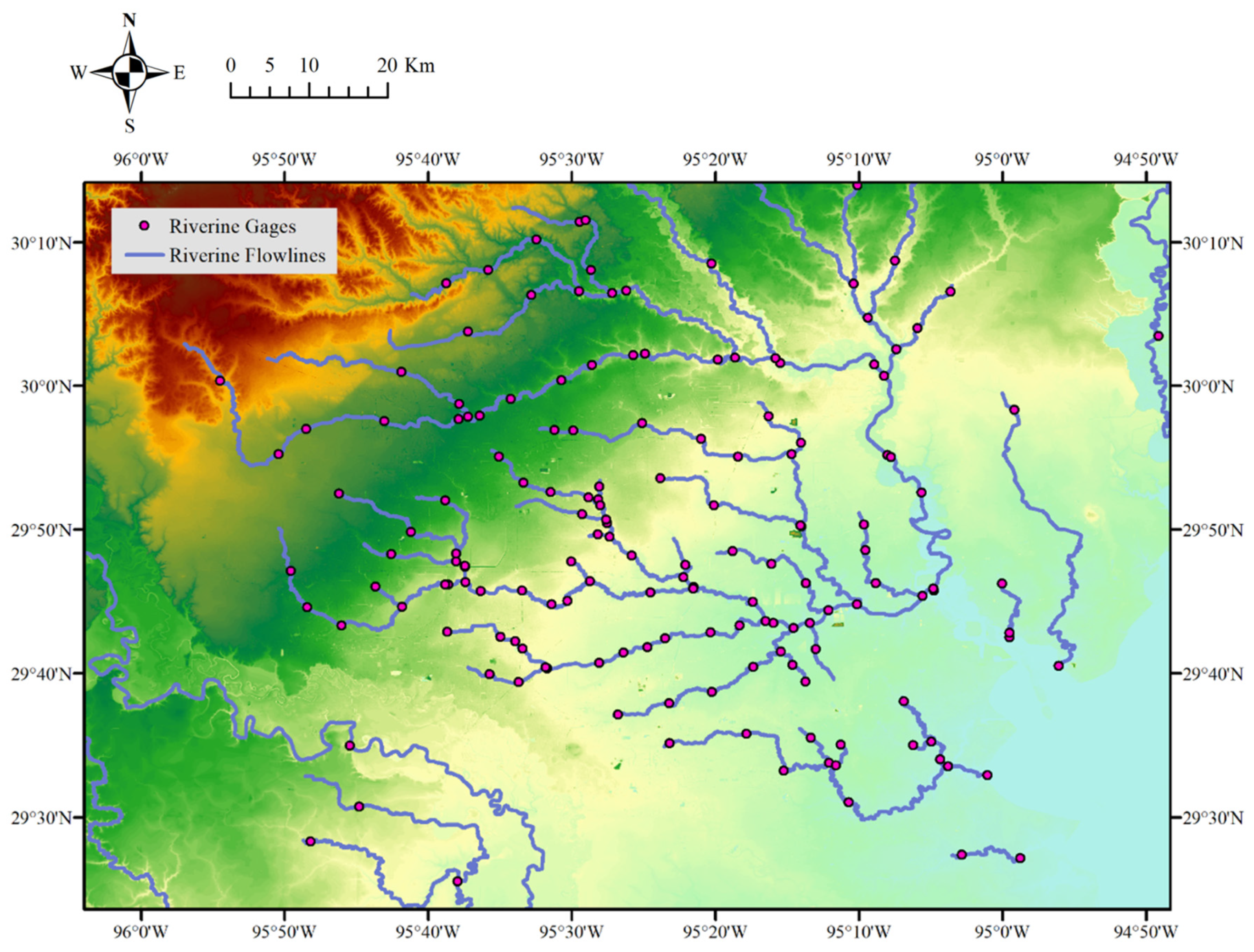
Gauges are spatially sparse so that information between existing gauges needs to be estimated by interpolation. The interpolation processing relies on the understanding of the hydraulic situation—how water flows on a terrain surface. To facilitate this interpolation, the National Hydrography Data flow lines are used to create reinforcement points. A flow line depicts the path of a stream or river, and the gauges are located along a river. While the flow lines link the gauges, points on the flow line intersections and between gauges are used as reinforcement points. Water levels of the reinforcement points are estimated based on the gauge’s readings and the distance to the gauges located on the upstream and downstream.
Once the water level elevations are available for the gauges and reinforcement points, a triangulated irregular network (TIN) is generated to represent the continuous water surface. This water surface is then converted to a raster image, with the same geo-reference and grid alignment as the ground DEM data. Overlaying the water surface with the DEM, flood depth can be calculated as the difference between the water surface elevation and ground elevation (similar to [29]). Flood extent is identified as regions where the flood depth is positive. For isolated flood areas, if they are not adjacent to gauges and reinforcement points, they are regarded as disconnected false flooding areas and are removed. The flooded region with depth information is the final product and denoted as the riverine flood depth. The flood depth is categorized into a multi-class set and is used as one spatial evidence to estimate the presence probability of flooding.
3.4. Storm Surge Simulated Water Height
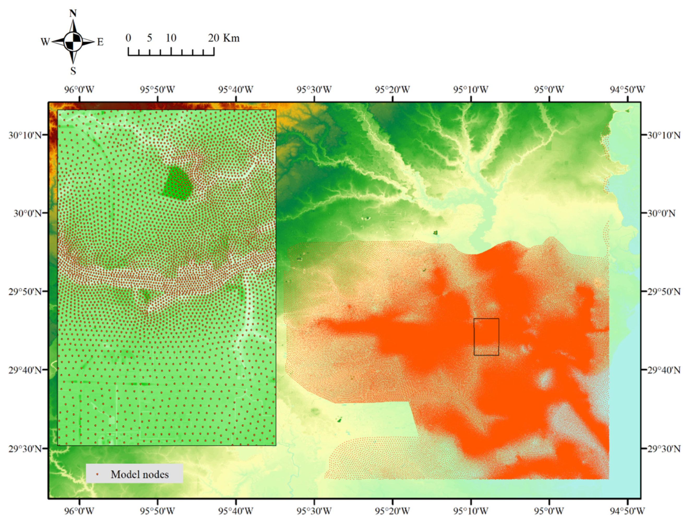
The Advanced CIRCulation (ADCIRC) model is a finite element model to forecast or estimate water height caused by storms [30,31]. Millions of elements are used in the domain of interest where the element sizes are various, ranging from ten meters along the coast to ten kilometers in the deep ocean. For each element, wind and pressure fields are required and obtained from multiple hydraulic data sources. The ADCIRC model outputs include water surface elevation and velocity over the domain continuously. This study makes use of the estimated water surface elevation to interpolate water height caused by storm surge for the study region.
The storm surge model nodes calculate water height continuously, and the daily maximum records are used to generate the storm surge surface. The dense point set is transformed into a continuous surface through Thiessen polygon creation. Although the point set is relatively dense, the discrete points could not be directly combined with the other raster data. Thiessen polygons, also known as Voronoi diagram, are generated from the point set, in which the polygons share the same value, here water height, as the center point. In a space , a Thiessen polygon surrounding a point could be expressed as
where the distance function used in this study is the Euclidean distance. After the Thiessen polygons are created and their values of water height are assigned, they are converted into rasters to match other data sets, regarding georeferenced and grid properties. Then the height is categorized as the riverine flood depth data using multiple quantiles of the total data.
3.5. Land Cover
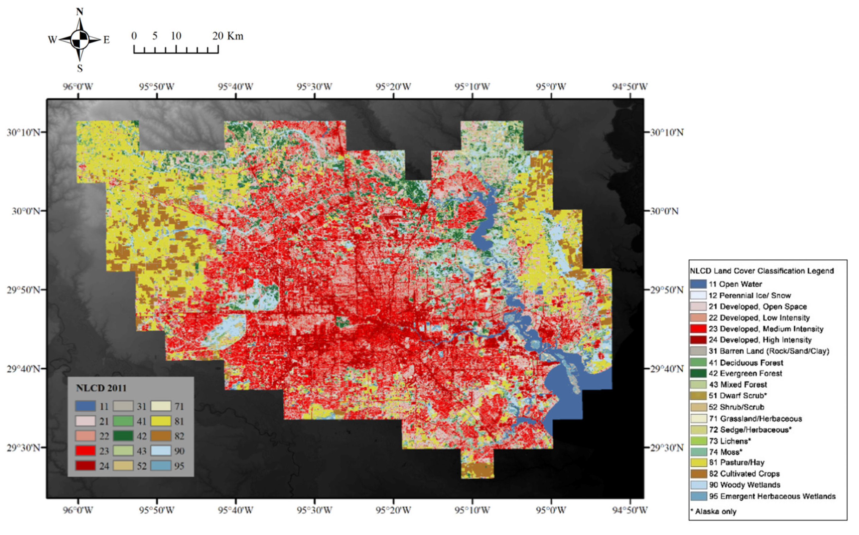
The land cover information is obtained from the National Land Cover Database (NLCD) at a resolution of 30 m [32,33]. According to the modified Anderson Level II classification system, there are 16 classes of land use and cover in the NLCD product. The Level I classification is used in this study to aggregate the land cover types, including water, developed, barren, forest, shrubland, herbaceous, planted/cultivated, and wetlands. Each land cover type is used as layers of spatial evidence.
3.6. Data Collection for Hurricane Harvey
In August 2017, Hurricane Harvey swept Southeast Texas as the wettest and costliest tropical cyclone. More than 1000 mm of rain was received in many regions over four days, with a peak of over 1500 mm rain accumulations. The catastrophic flooding caused the death of over 100 people, displacement of more than 40,000 people and damage worth over 125 billion US dollars, according to the National Oceanic and Atmospheric Administration (NOAA). Harvey was formed on 17 August 2017, moved towards the northwest and made multiple landfalls. With an intensification phase of a Category 4 hurricane, Harvey made landfall on 25 August at San Jose Island and Holiday Beach, after leaving Barbados and Saint Vincent. After that, a torrential downpour of rain led to unprecedented flooding. Oil refineries were shut down, declining energy production, and some chemical plants suffered from explosions due to a power outage [10]. On 2 September, Harvey weakened and dissipated.
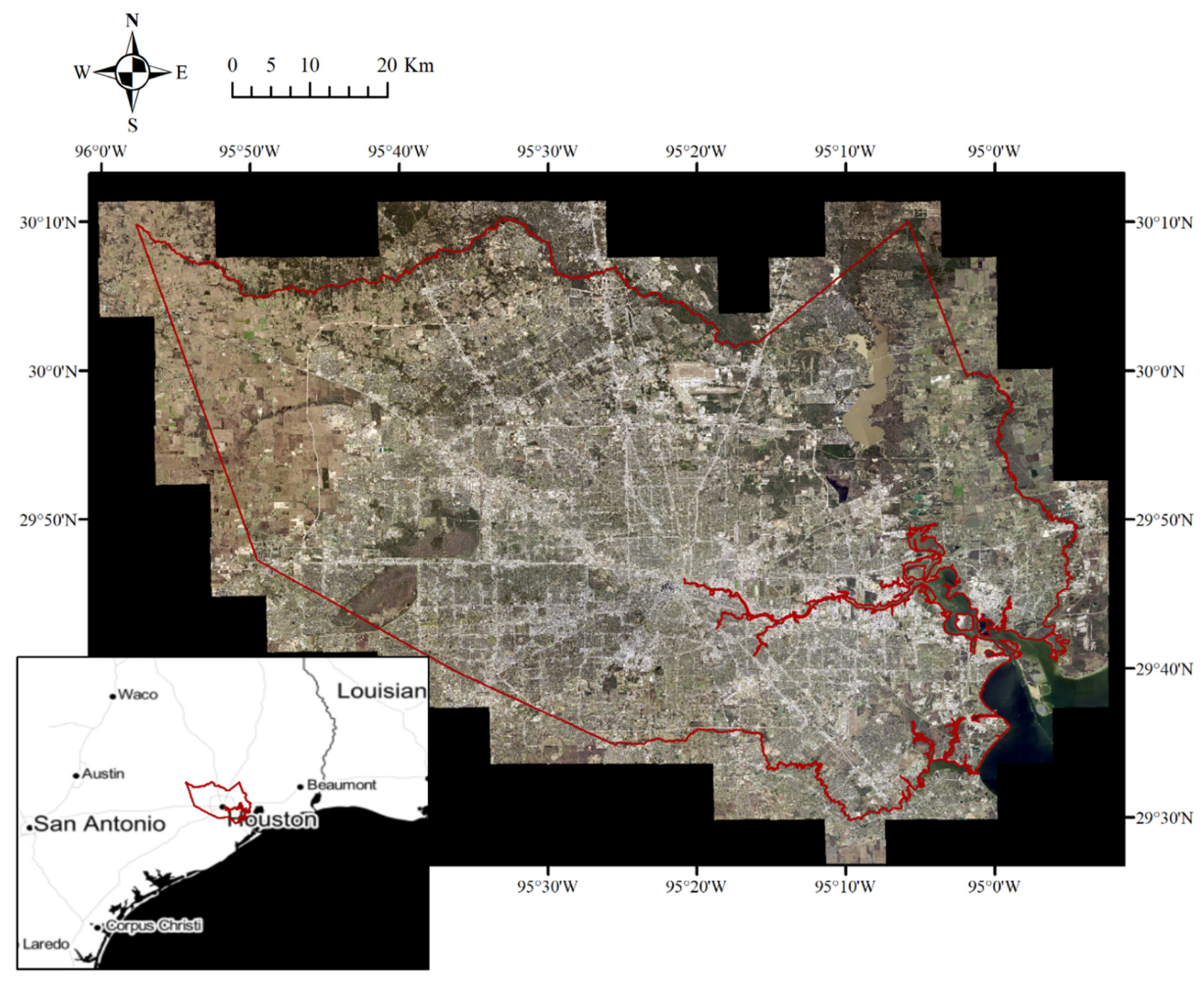
In Texas, the Department of Public Safety estimated that about 300,000 structures and 500,000 vehicles had been destroyed or damaged [4]. Houston metropolitan areas observed over 990 mm of precipitation during August, the wettest record since 1892. On 27 August, the National Weather Service office in Houston measured 408 mm of daily rainfall accumulations. Emergencies of flash flooding were issued several times from 26 August onwards. Harris County Flood Control District estimated that 25–30% of the county was submerged, around 450 square miles. The regions in Figure 1 are investigated, including the Addicks and Barker Reservoirs in the left part. These reservoirs were built by the US Army Corps of Engineers with aims to prevent flood damages to the city of Houston.
Harris County is the site of interest in this study, shown in Figure 1. According to the US Census Bureau, Harris is the most populous county in Texas and ranked third in population across the country, home to 4.5 million people. The county seat, Houston, is the fourth largest city in the U.S. In Figure 2, developed areas with different intensities are depicted in various shades of red (Land Cover Class 21–24), making up a large portion of the county area.
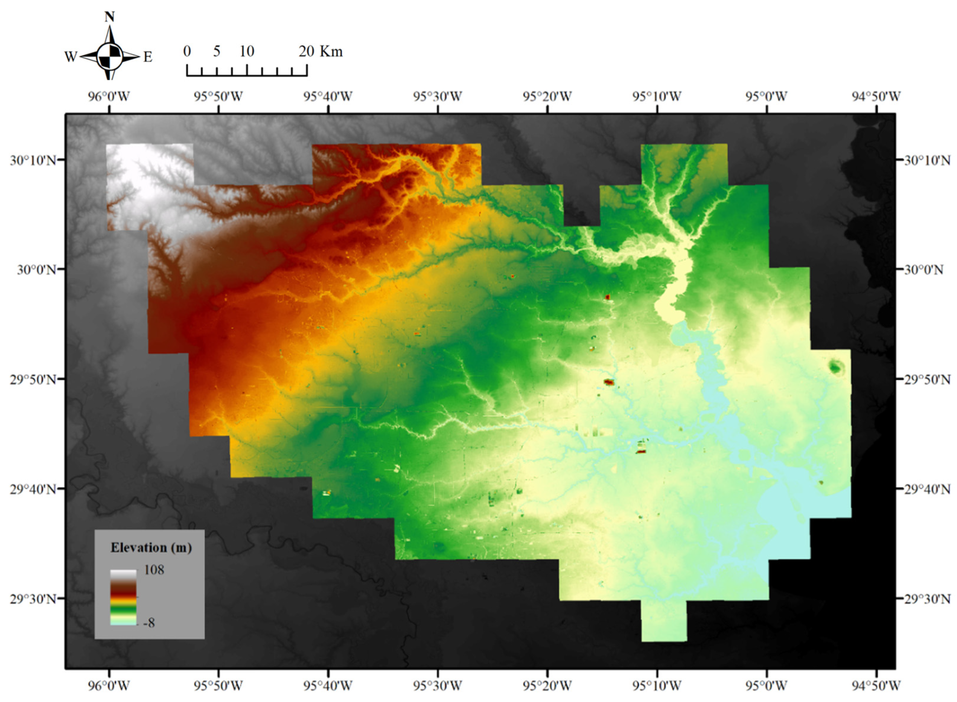
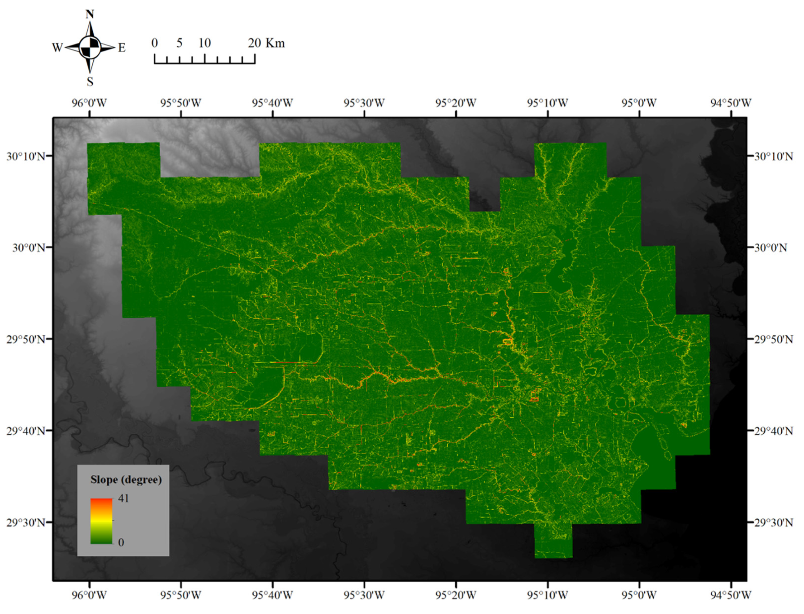
Located in the Gulf Coastal Plain, the region of interest is mainly made up of clay-based soils and it is low-lying. The digital elevation model and the derived slope are shown in Figure 3 and Figure 4. The northwest part is higher in elevation than the southeast part where most rivers and streams flow. The slope is usually small, except along the mountain ridges and the river banks. This area is a vast floodplain depending on San Jacinto River and Buffalo Bayou to carry away flood and stormwater.
The digital elevation model (DEM) was collected from the National Map 3D Elevation Program, and the source data are products of LIDAR point clouds, with a spatial resolution or ground spacing of 10 m. Based on the DEM, the slope is determined by the change rate of the surface in vertical and horizontal directions. An increase in slope suggests that the terrain is changing from a relatively flat state to a steeper state. As water flows from regions of high elevation to low elevation and usually is trapped in flat areas, the slope is a reasonable indicator of inundation. However, for this study site, a large portion of the area is of a very small slope, so this may not add much useful information as a spatial evidence layer.
The riverine floodplain and depth were calculated using gauges and flow lines shown in Figure 5. The nodes to simulate storm surge by the ADCIRC model are shown in Figure 6, with an enlarged frame for the dense points. Notice that the storm surge simulation could not provide full coverage of the study site and it is available for the coastal regions.
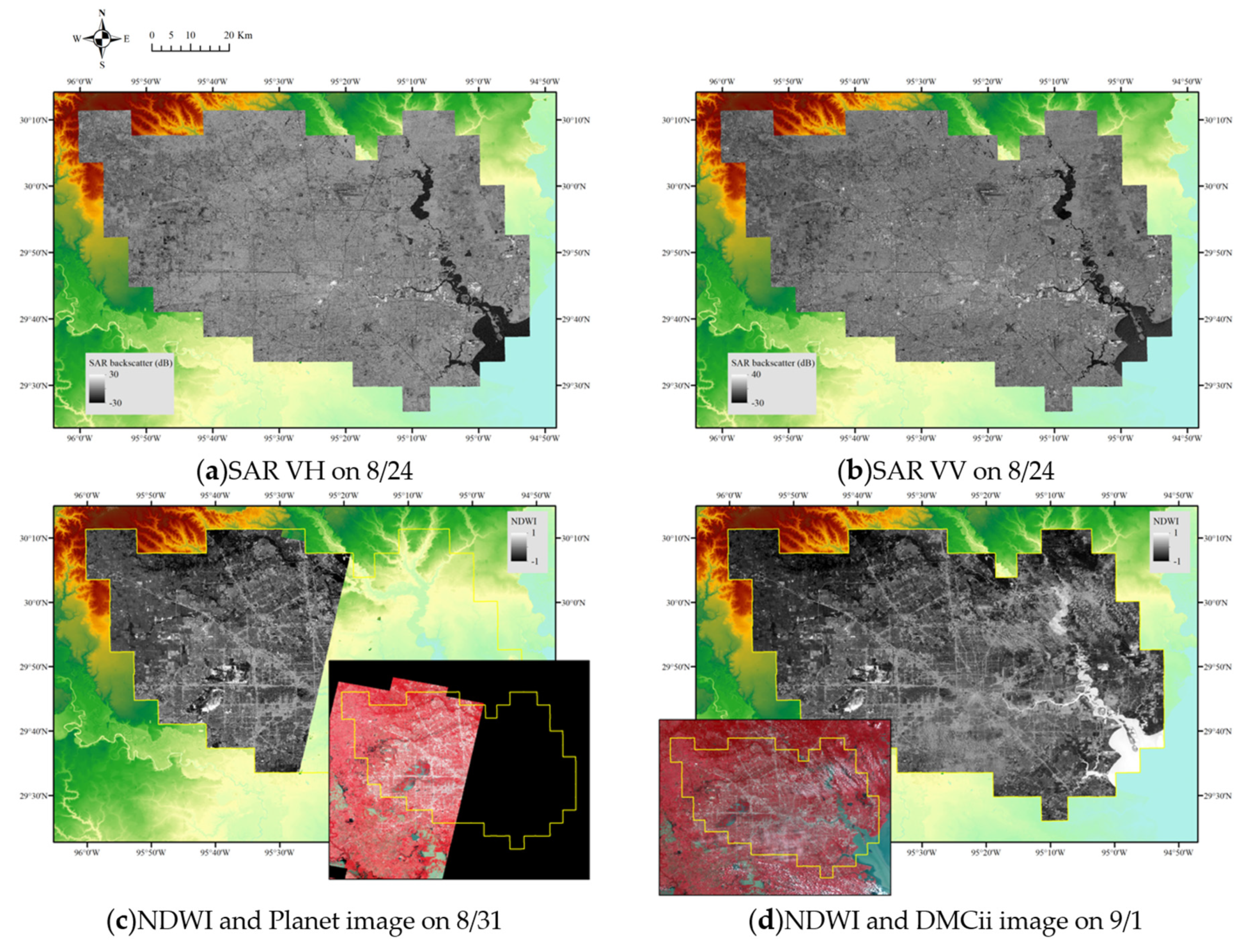
The riverine flood depth was collected and processed on 27–30 August, and 1 September (list in Table 1). The ADCIRC model outputs, simulated water heights, were collected and processed as the previous section from 27 to 30 August. As shown in Figure 7, the SAR images were acquired from Sentinel-1 on 18, 24, 30 August, and 5 September; the Planet and DMCii images were used to calculated NDWI on 31 August and 1 September. The Planet image could not cover the whole study region, missing the eastern part. The inundation areas were detected using the satellite images (Planet and Sentinel-1) and support vector machine classification with manually selected training samples. Then the inundation extent was used to estimate the weights of different spatial evidence based on the Bayesian conditional probability framework (Section 2.1).
To assess the estimated inundation, satellite images and flood maps from multiple data sources were used as the ground reference, including supervised classification on the high-resolution optical image from DMCii and flood maps released by FEMA.
4. Results
In this study, the water extent derived from the satellite image acquired on August 30 (Sentinel-1) and 31 (Planet) was used to estimate the weights of various spatial evidence, and the resulting weight of evidence is listed in Table 2. Each evidence layer is divided into multiple subsets, according to quantiles or land cover types. As the riverine flood depth and the storm surge water height can be available daily, the depth and height of the day that the remotely sensed image was acquired are used to generate the multi-class evidence layers. The ranges of different variable classes are also included in Table 2, which correspond to quantiles of the spatial evidence or land cover types. Regions of low SAR backscatter intensity (for both polarization), high NDWI, flood depth or storm surge height have larger positive weights and contrasts , indicating possibilities of positive spatial association. The areas with SAR backscatter intensity below −18 dB for polarization VH (vertical transmit, horizontal receive) and below −25 dB for VV (vertical transmit and receive) are possibly open water. In addition, open water (Land Cover Class 11) and bare soil (31) are also highly related to inundation, having positive weights of 4.45 and 1.42. Grassland (71) and cropland (82) are less relevant (weights lower than 0.25). The standard deviations of weights and contrast are small, thanks to the large sample size (amount of image pixels). The studentized contrast is used to determine the final weights of spatial evidence, with a bold value in Table 2, suggesting the final weight selected to calculate inundation probability. Since the five types of spatial evidence are assumed to be positively related to inundation, only positive weights are used for the presence of spatial evidence. As mentioned in Section 2, the variance of the posterior probability could be estimated by the variance of weights by Equation (13). The variance of weights, listed in Table 2, are small, ranging from to . Based on Equation (13) and the calculated variance of weights, the variance of inundation probability is small.
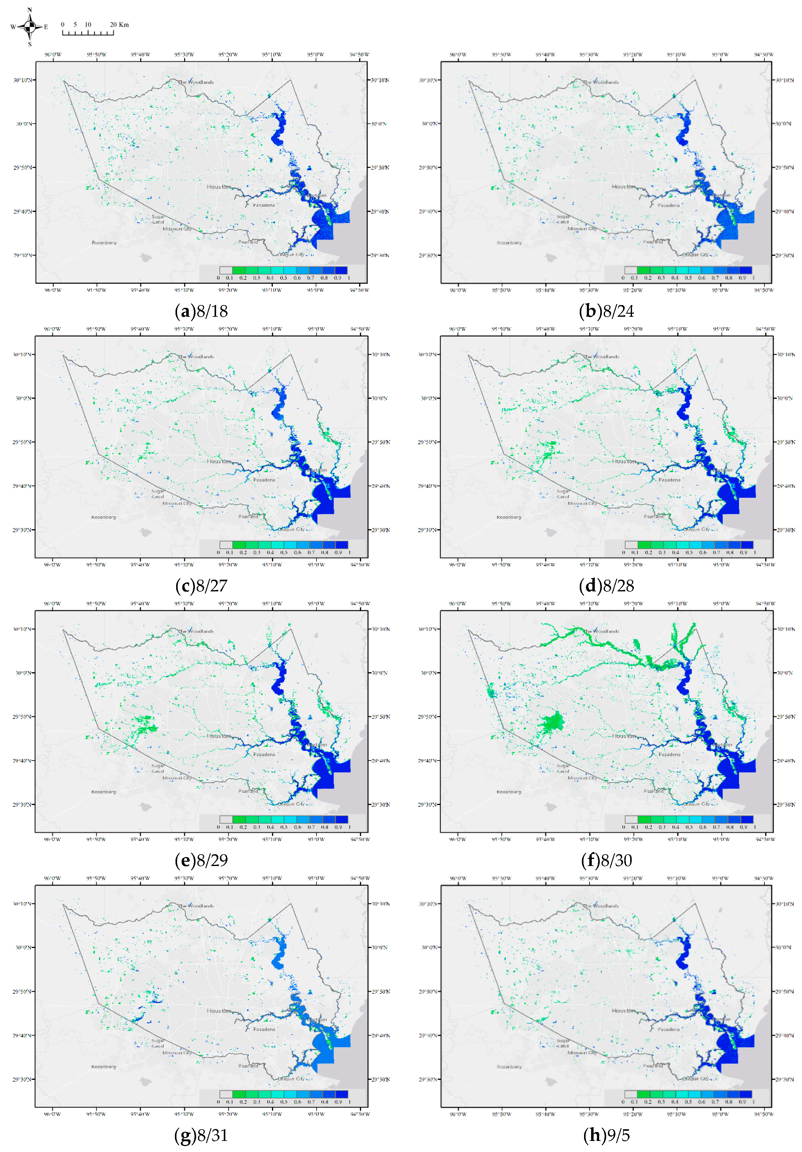
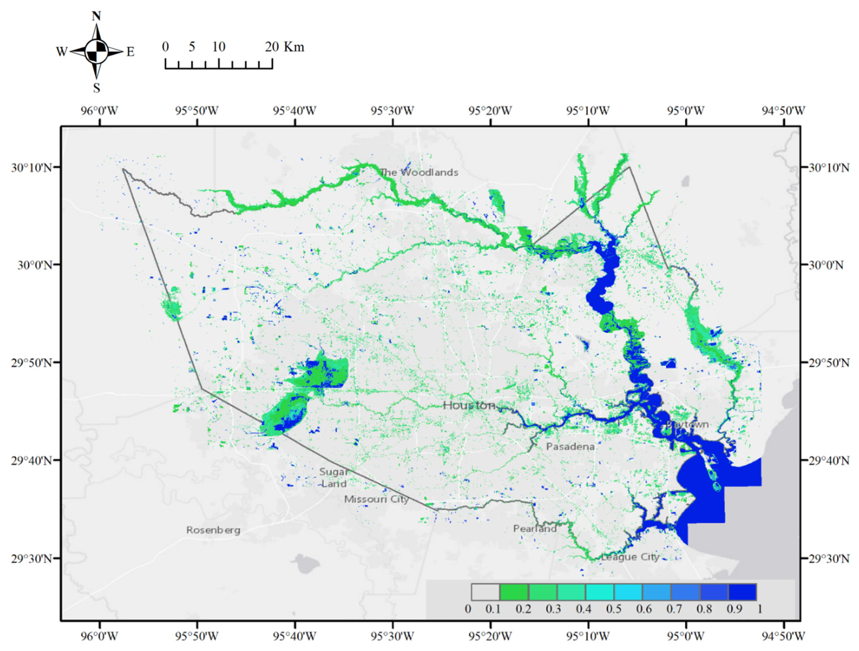
The predictor map, the posterior probability of inundation, is obtained by combining the presence of different forms of spatial evidence and their weights. The prior odd of inundation is estimated as the ratio of open water to the total area of interest. In Figure 8 and Figure 9, the posterior probabilities of inundation are shown for Harris, Texas, on 18, 24, 27–30 August, and 1 and 5 September 2017. During this period, the water extent increased and submerged areas could be found along the rivers and streams, and around the reservoirs (Addicks and Barker Reservoir). From 27 August (Figure 8c), flood water could be found near the center of Houston, along the streams. From 18 August to 1 September (Figure 8d–g and Figure 9), inundation probability around the two reservoirs was increased. However, the inundation evolution is not smooth. The water area near the reservoirs expands in Figure 8d–f, with relatively low inundation probability. In Figure 8g, the water area decreases but the inundation probability increases. This inconsistency may be due to data availability. River stream gauge data are available from 28 to 30 August and 1 September, the storm surge model 28 to 10 August, and satellite data from 30 August to 1 September. Except for 28 and 29 August, the daily data availability is different, even for two consecutive days. Such a difference in data availability and data quality could lead to the inconsistency of estimated probability.
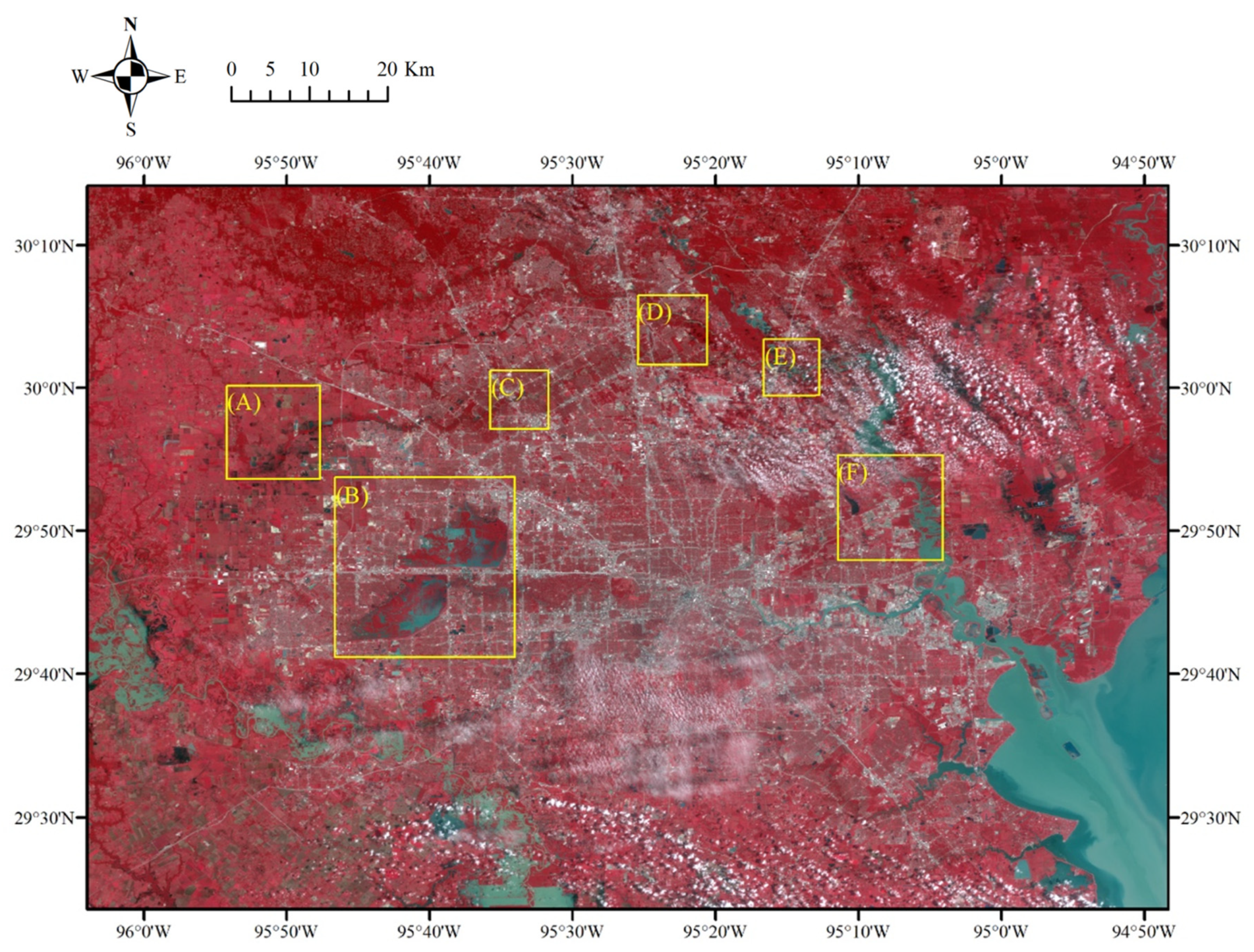
There is no available storm surge simulation on 1 September, so the inundation probability map (Figure 9) is generated by remote sensing data, riverine flood depth, and land cover data. An optical image is used to assess the effectiveness of the method. This image was collected by DMCii with a multi-spectral sensor and a spatial resolution of 22 m. Six locations in Harris are selected to show detailed water distribution, as in the yellow boxes in Figure 10.
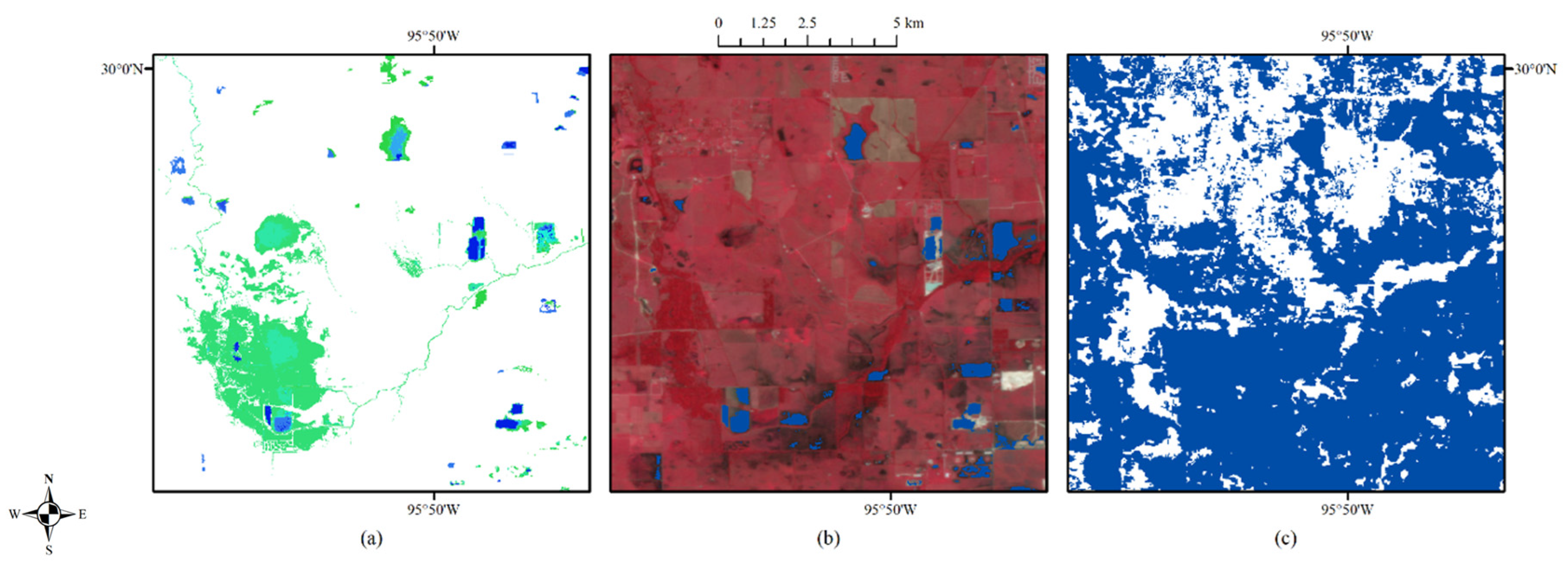
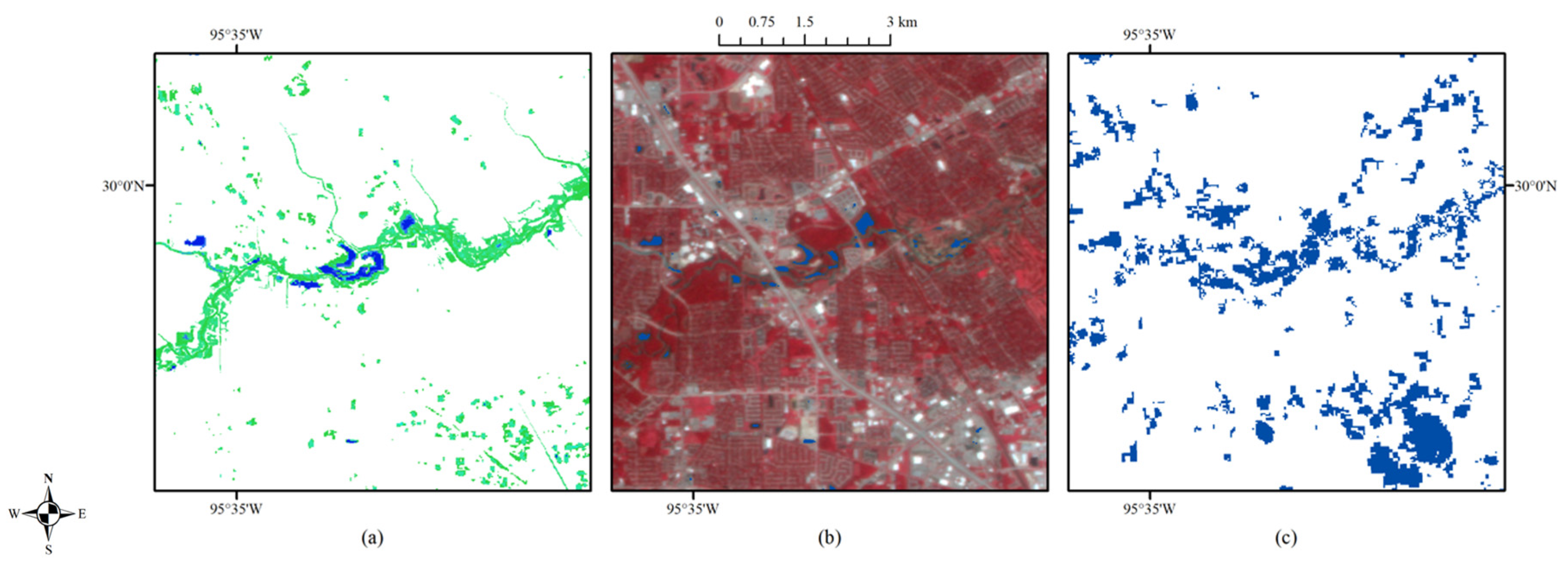
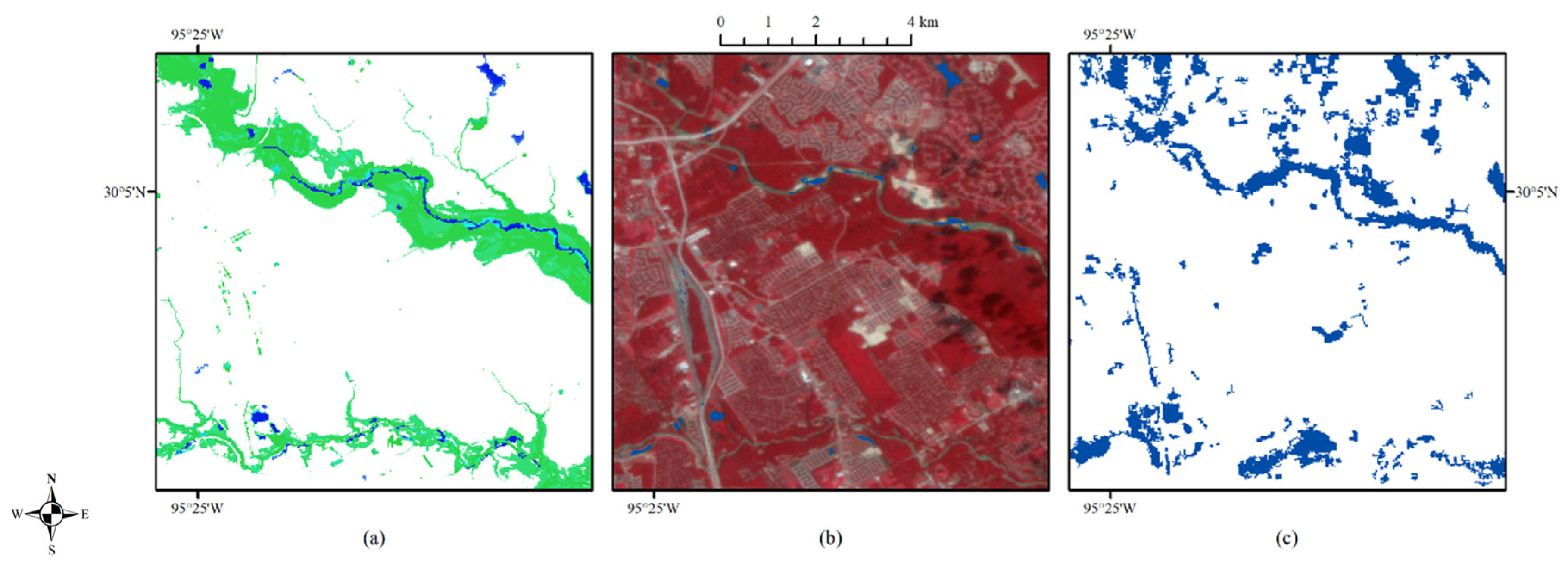
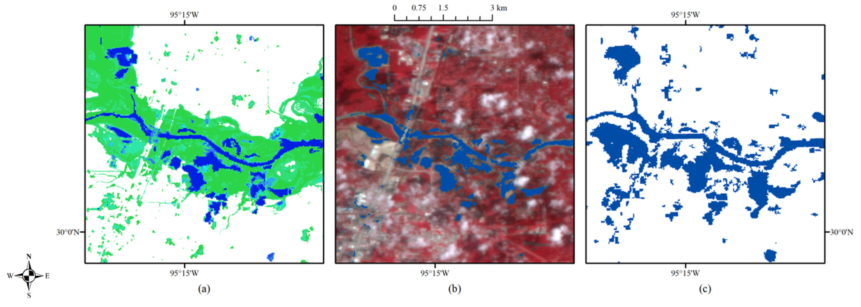
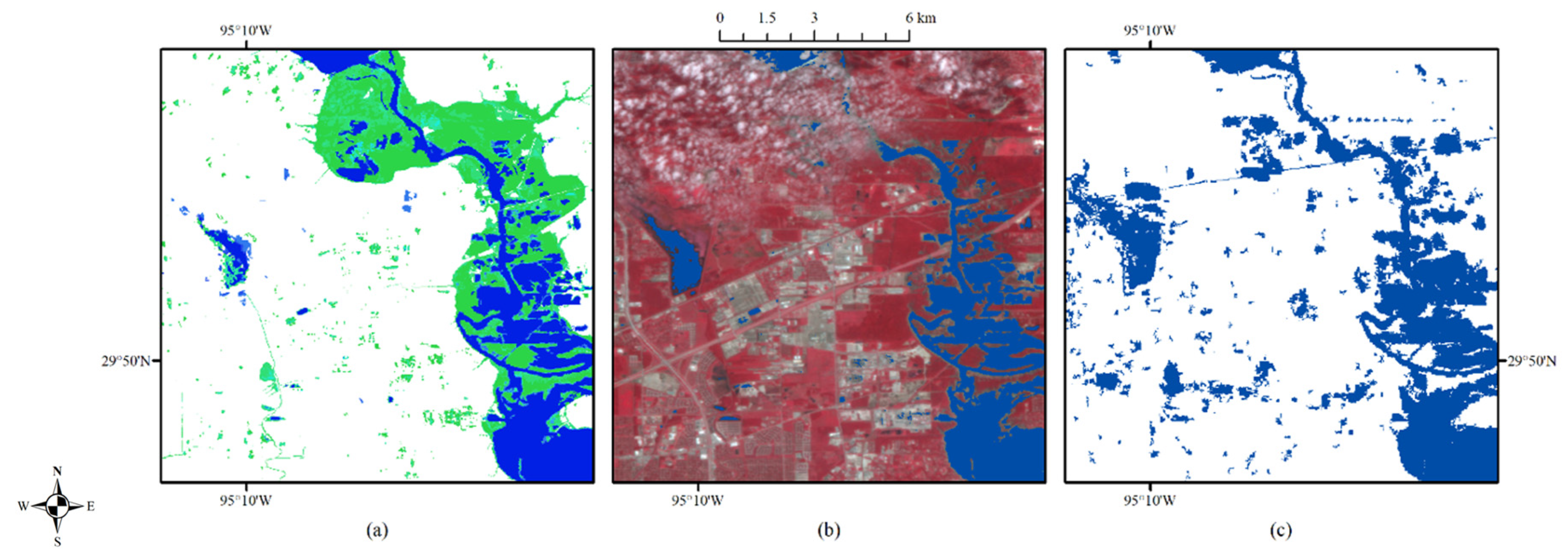
As shown in Figure 11, Figure 12, Figure 13, Figure 14, Figure 15 and Figure 16, the validated water extent (blue areas in (b)) agrees well with the regions of inundation probability larger than 0.9. The estimation generated from the proposed method is more accurate than the FEMA flood map, which tends to overestimate the water extent.
Figure 12 shows the Addicks Reservoir and the Barker Reservoir, which is a ‘dry’ reservoir covered by vegetation usually. From these two reservoirs, water was released with control towards the Buffalo Bayou after 28 August. Despite the original attempts to protect the neighboring area, the Addicks Reservoir began to spill out after reaching its capacity. The recorded water level during Hurricane Harvey was the highest since the construction of the reservoirs.
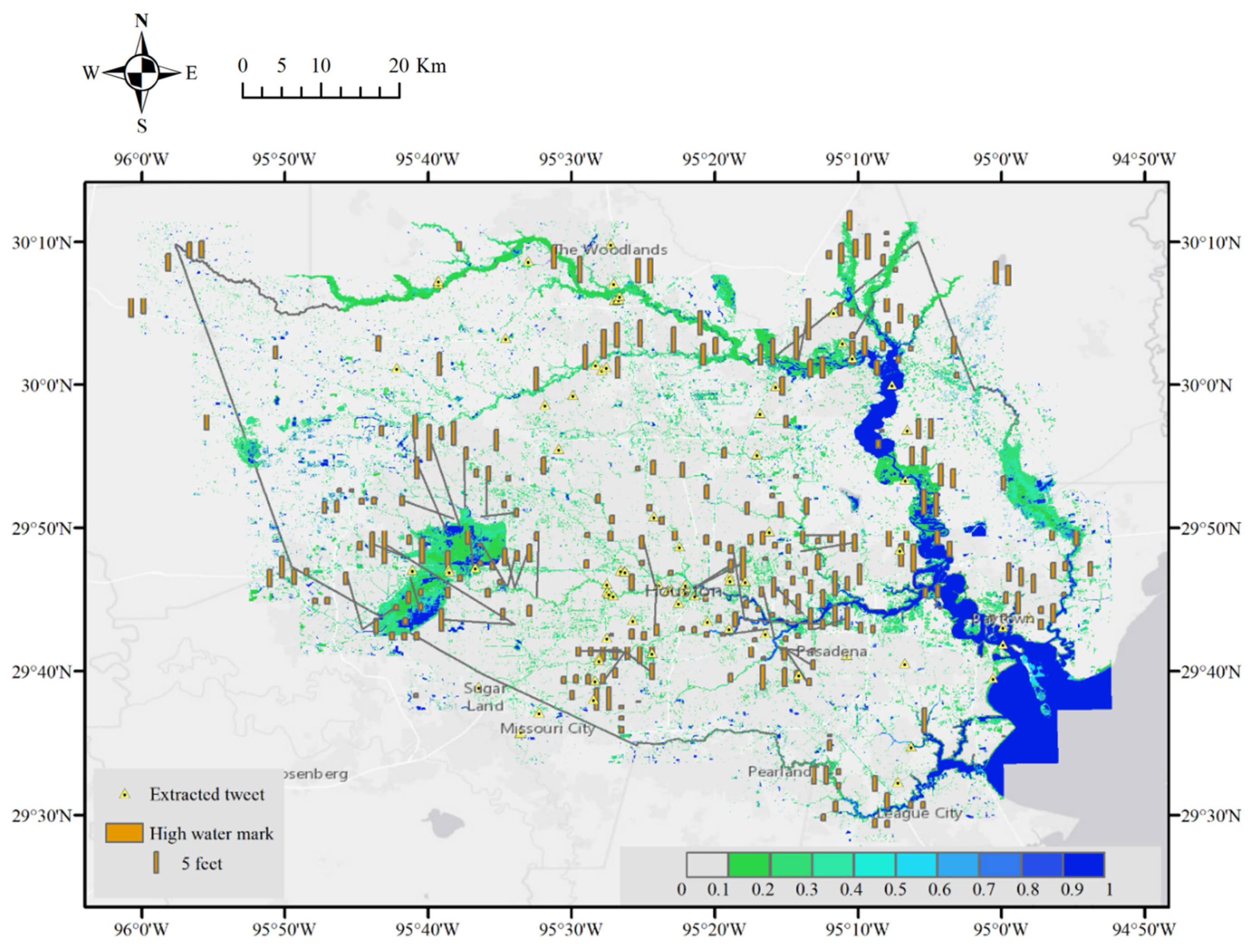
Based on the time series maps from 18 August to 5 September (Figure 8 and Figure 9), the maximum estimated inundation probability for each pixel along the time series is produced and shown in Figure 17, along with extracted tweets and high water marks. The observed points are usually inside or near the regions of high inundation probability, especially around the streams or large water bodies. For the areas with low inundation probability, if those regions are at high flood risk, for example, places with a short distance to the river and with low elevation, inundation could be possible. However, the low inundation probability in potential flooded urban areas implies a major limitation of the proposed fusion method.
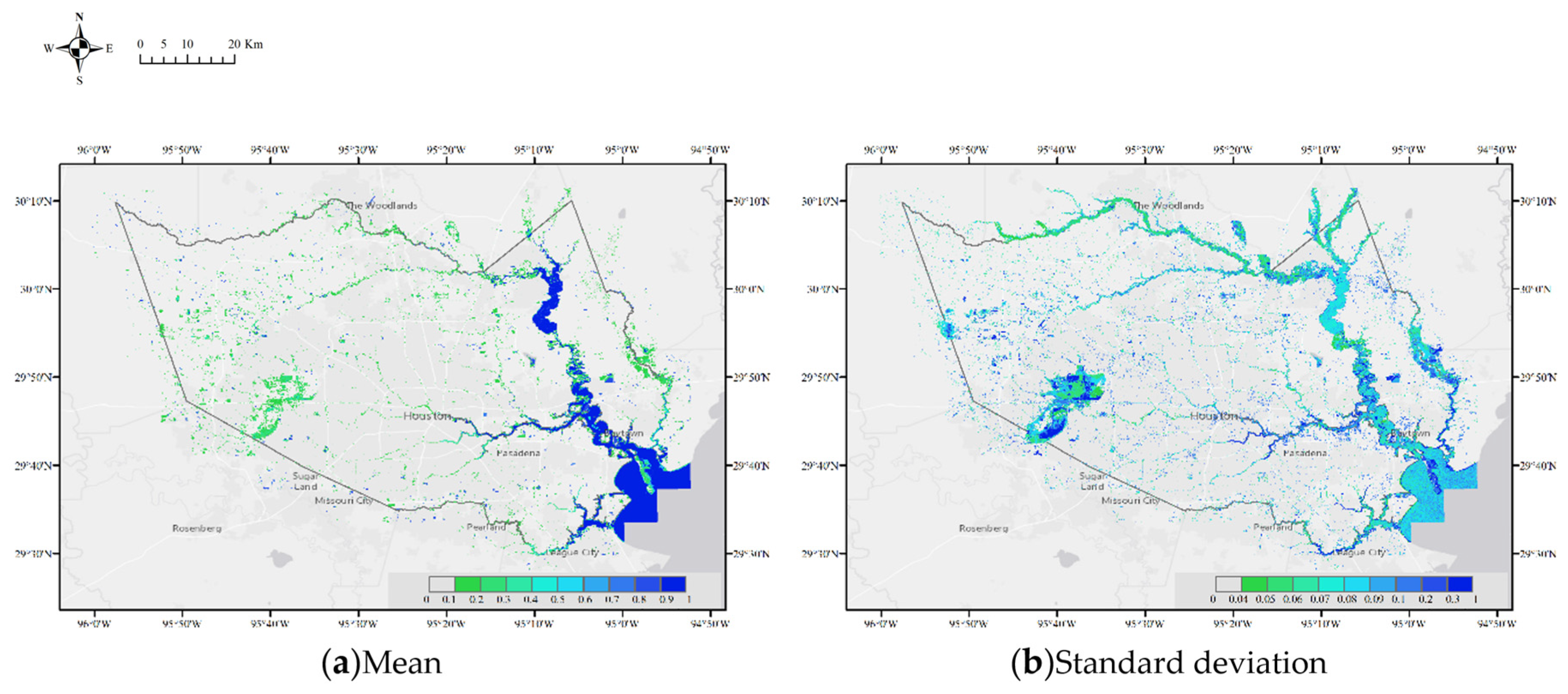
Similarly to the calculation of maximum inundation probability, the mean and standard deviation are also calculated and shown in Figure 18. High mean inundation probability suggests normal or permanent water, and areas of high standard deviation are generally flooded regions where surface water is uncommon. Using the maps of mean and standard deviation, flooded regions with severe impact could be identified, such as Addicks Reservoir, Barker Reservoir, and the riverside near downtown Huston.
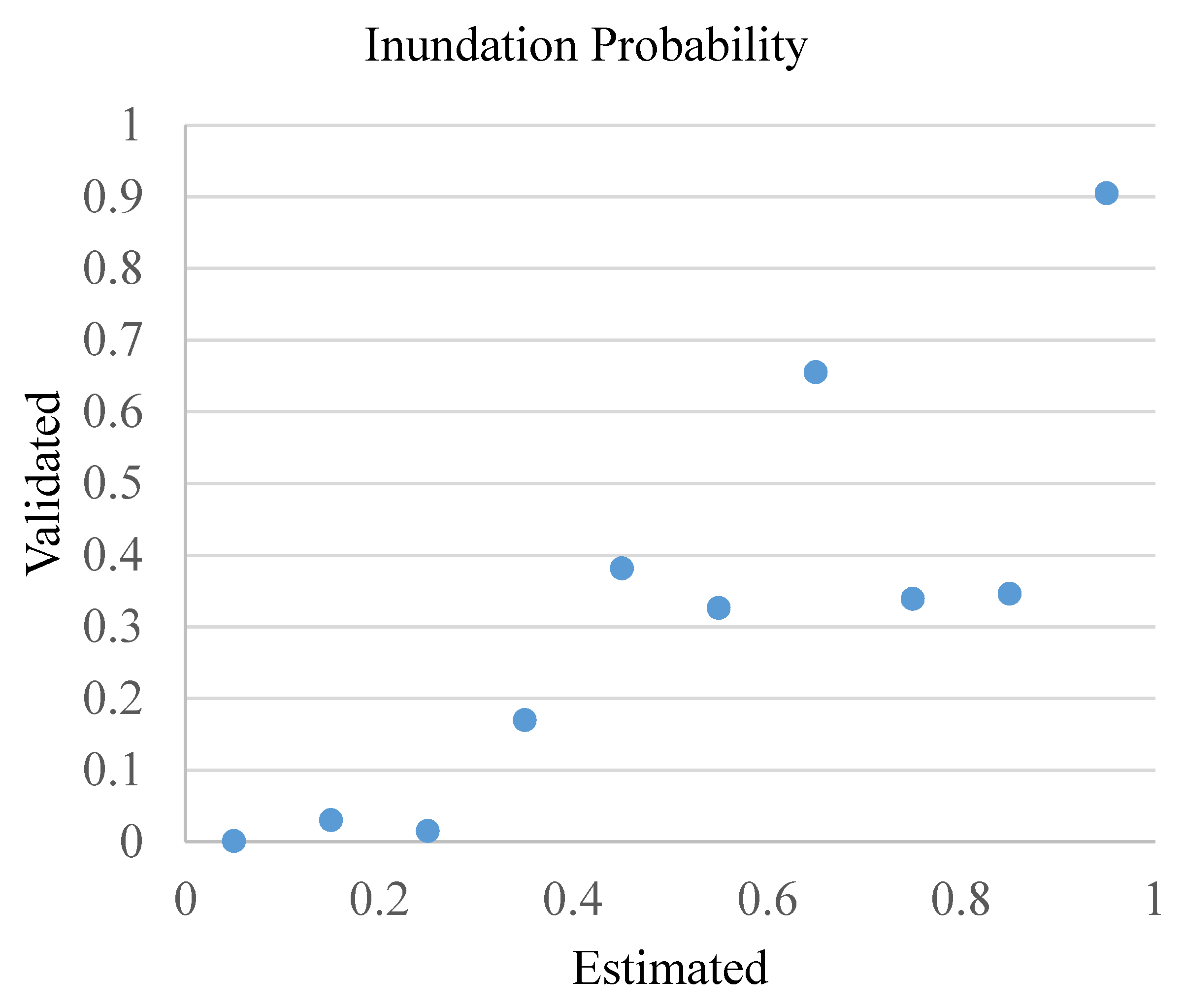
A reliable diagram of 1 September (Figure 19) is used to quantitatively assess the prediction. The probability range is split into ten intervals . Pixels of estimated probability within each interval form a subset, and in such a subset, the validated water extent ratio is used as the validated probability. Generally, the prediction is close to the validation, especially for the regions with relatively small (<0.5) or large (around 0.7 and 0.9) inundation probability. Though the prediction reliabilities of intervals and are lower than other intervals, the pixel amount of these intervals is rather small, as listed in Table 3. In order to consider the pixel number, the weighted root-mean-square difference was calculated, with a value of 0.0686.
5. Discussion
In this paper, we proposed a framework to fuse multi-source information to generate daily maps of inundation probability. We incorporated remote sensing data, riverine flood depth, storm surge simulation, and land use and land cover. The fusion framework makes use of available data of a given day, because the multi-source data could not be acquired with the same frequency. In line with previous studies [11,12,13,14,15,16,17,18], the remotely sensed inundation extent is clearly useful to observe flood events, but such a technique could be sensitive to the timing of image acquisition. The SAR images used in this study are theoretically accessible every six days, but observation gaps still exist. The optical images, though more informative, are limited due to heavy cloud coverage, which is often present during a flood event. When the optimal data sources are limited, we utilized other information sources and provided a series of consistent probability maps. We found that each data source has some limitations and uncertainty, but the fused result is more accurate than each component in terms of identifying the inundation extent. The estimated inundation probabilities using fused components are more realistic than the ones using a single data source.
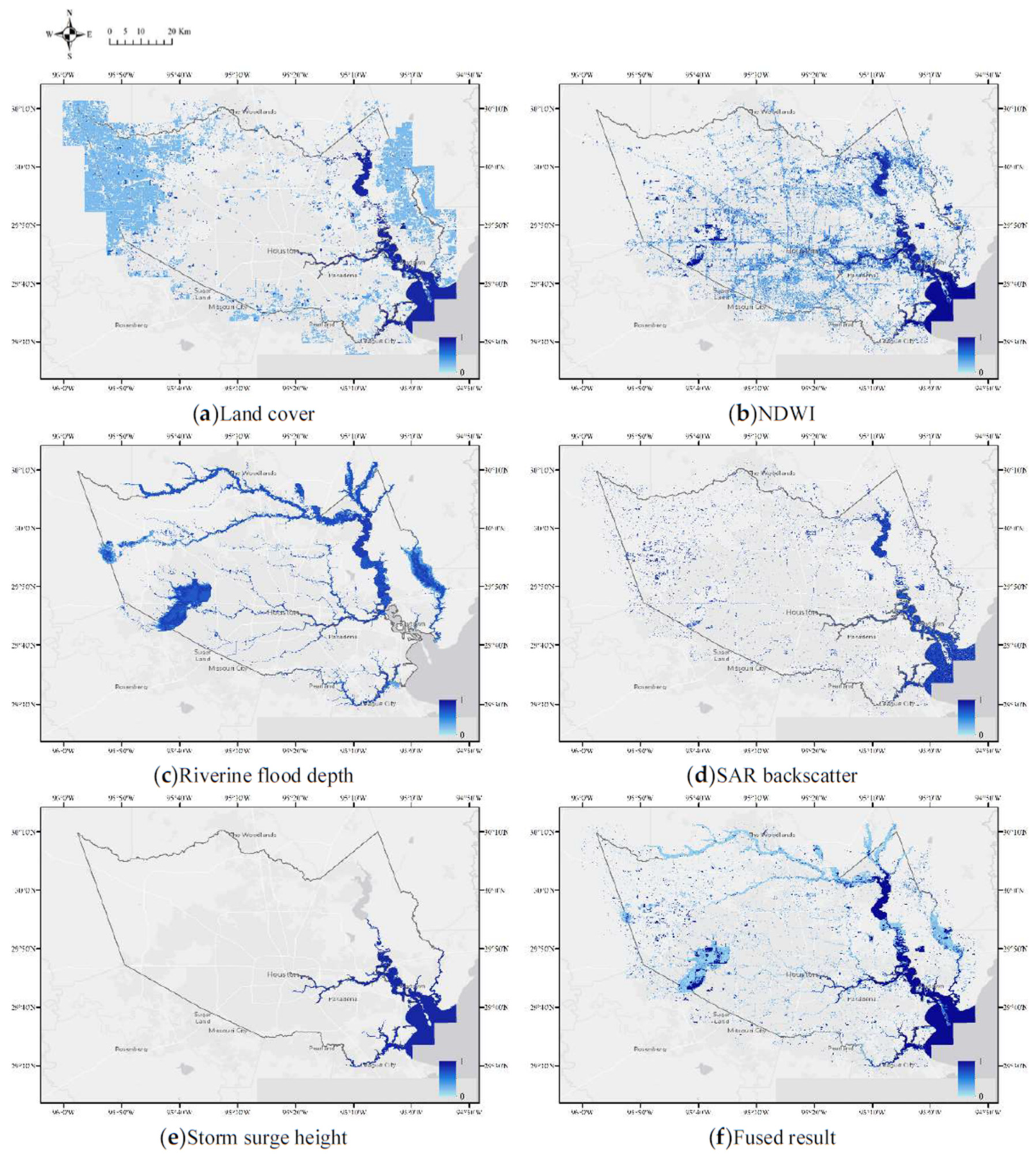
Each data source has limitations in mapping inundation. In Figure 20, the light blue regions indicate areas of high uncertainty. The land use and land cover data are static during the flood evolution, so the probabilities estimated from the land cover are also constant for different days. Areas with high probability in NDWI and SAR backscatter are correlated with the high probability areas in the fusion result. In this study case, NDWI estimates an extensive area of rather low inundation probability. SAR backscatter estimates less water extent but with higher inundation probability than that from NDWI. Although the probability maps estimated from NDWI and SAR backscatter are for different days, the difference in probability could be dramatic for the same event.
The riverine flood depth relies on the estimation of water surface elevation, which could inevitably include some inaccuracies or even errors. First, gauge readings are usually fairly accurate, but on the one hand, not every record is uploaded and usable. On the other hand, the daily highest water level may not correspond to the water level of the flood crest. Second, interpolation based on gauges and reinforcement points may not capture the reality among areas without reliable observation. Third, flood depth calculation using DEM would suffer from the propagated error of the input data. Lastly, the removal of isolated flooded regions could ignore some actually flooded areas.
Similarly, the water heights simulated by the storm surge model have their uncertainties from input data qualities and modeling reliability. Furthermore, the transformation from storm surge nodes (points) to surface (raster) via Thiessen polygons might have some local issues. For example, the boundaries of river banks or coasts show artifacts with abrupt transitions. More complex interpolation and post-processing considering topography could be helpful. One possible solution would be using the initial storm surge model mesh to interpolate water heights, but given the fine resolution in the coastal mesh, the improvement may not be significant. Nevertheless, the Thiessen polygon generation would be more efficient for near-real-time or real-time applications, because one set of polygons could be applied to the flood event for a few days or even months, without repeating interpolation processes.
The fused result (Figure 20f) is a statistical combination of the different components (Figure 20a–e). In the Results section, we compared the estimated inundation probability with the remotely sensed water extent and observation points (flood Tweets and high water mark). Areas with high probability tend to be flooded (Figure 11, Figure 12, Figure 13, Figure 14, Figure 15 and Figure 16). However, observation points can be found near places of relatively low probability, especially in the city center. This is a major limitation of the proposed method. Although the observation points are not evenly distributed and of different scales (much higher resolution than the spatial evidence layers), the points are reliable data showing water presence. The overlaid map of points and probability shows that regions with low probability can be flooded when those regions are at high flood risk. Future studies can consider flood risks, such as distance to rivers or low-elevation places, modeled flood return period, and historic flood frequency. In addition, additional data in urban areas can be beneficial, including sewer systems and SAR interferometry coherence.
We also tried to include elevation and slope information but later found that the elevation-based information could not improve the results. The weight of evidence modeling assumes conditional independence among different predictors. Since the elevation data were used to calculate riverine flood depth and slope, the elevation and slope do not provide additional information as other independent spatial evidence.
The spatial evidence layers used in this study are assumed to be independent as they are collected from independent measurements. These layers are combined through a probabilistic approach so that a higher probability value suggests a lower level of uncertainty. However, the uncertainty over each day of the time period varies for different places, because the availability of spatial evidence layers is different most of the days. Another issue that has not been addressed is the propagation of uncertainty in calculating inundation probability. Although the measurements of remote sensors and river gauges are assumed to be accurate enough, the weights of spatial evidence are calculated for non-overlapped subsets of each layer. For example, the final weight of river flood depth between 5.96 and 8.15 feet is 0.27, and of depth between 8.15 and 10.36 feet is 1.82. Within a subset (e.g., 5.96–8.15), the uncertainty is assumed to be even. Areas of flood depth 8.14 and 8.16 feet have quite different final weights (0.27 and 1.82). Consequently, uncertainty may propagate from layer preprocessing, so layer value could end up falling in a less reliable weight.
In Harris County, Texas, only 15% of homes have flood insurance, according to the National Flood Insurance Program (NFIP). Meanwhile, flooding has been common since the founding of Houston; for example, the previous floods in May 2015 and April 2016. Houston had been submerged by three 500-year floods in three consecutive years before Harvey. Due to the lack of planning and zoning restrictions, Houston’s urban sprawl is astonishing, even within floodplains. Around the reservoirs in Harris, the population increased from 400,000 in the 1940s to six million in 2017. To address the increasing challenge from environment and society [34], mitigation and adaptation measures, including seawalls, levees, and building codes, need to be employed. All these measures need to be informed by timely and continuous inundation maps. As disasters like Harvey will happen with increasing frequency and intensity, mitigation and adaptation are required based on an understanding of event evolution. By providing the inundation probability, this study could be readily implemented.
6. Conclusions
Extreme precipitation and sea level rise in a warming climate are aggravating flooding—a billion-dollar disaster, as called by the NOAA. Flood response, mitigation and adaptation require a comprehensive understanding of inundation evolution, yet our flood observations are limited regarding spatial and temporal coverage. This study tried to improve flood detection and observation in coastal areas by combining current satellite remote sensing-based techniques, in situ information from gauge measures, and storm surge model outputs. We proposed a fusion framework to integrate available information based on Bayesian conditional probability. The fusion product is a daily inundation probability map utilizing all accessible data. The input data could be different for each day, but the output is consistent within the probability range . Probabilistic flood maps could incorporate uncertainty propagated from the input data. The maps are useful for rapid response when important decisions such as collecting emergency aid or relocating residents need to be made.
Although this proposed methodological framework could provide useful results for the case studies, there are several limitations regarding input data uncertainty and error propagation. The accuracy of the proposed flood mapping methods varies in different regions of an image, but the error models between geographic characters have not been investigated. Lacking such information about the error, the generalizability of the proposed algorithms would be limited. The fusion model was trained locally for one study site, so additional consideration would be necessary when transferring the model to new sites.
Author Contributions
Conceptualization, J.L. and D.L.; methodology and validation, J.L. and D.L.; writing—original draft preparation, J.L.; writing—review and editing, D.L.; funding acquisition, D.L. All authors have read and agreed to the published version of the manuscript.
Funding
This research was funded by National Science Foundation Award, grant number 1520870 “Hazards SEES: Social and Physical Sensing Enabled Decision Support for Disaster Management and Response”.
Acknowledgments
We would like to thank Ethan Kubatko, Srinivasan Parthasarathy, and Steven Quiring for their comments in developing this study.
Conflicts of Interest
The authors declare no conflict of interest. The funders had no role in the design of the study; in the collection, analyses, or interpretation of data; in the writing of the manuscript, or in the decision to publish the results.
References
- Shultz, J.M.; Galea, S. Mitigating the mental and physical health consequences of hurricane harvey. JAMA 2017, 318, 1437–1438. [Google Scholar] [CrossRef] [PubMed]
- Rappaport, E.N. Fatalities in the United States from Atlantic tropical cyclones: New data and interpretation. Bull. Am. Meteorol. Soc. 2014, 95, 341–346. [Google Scholar] [CrossRef]
- Jonkman, S.N.; Maaskant, B.; Boyd, E.; Levitan, M.L. Loss of life caused by the flooding of new orleans after hurricane katrina: Analysis of the relationship between flood characteristics and mortality. Risk Anal. 2009, 29, 676–698. [Google Scholar] [CrossRef] [PubMed]
- Jonkman, S.N.; Godfroy, M.; Sebastian, A.; Kolen, B. Brief communication: Loss of life due to Hurricane Harvey. Nat. Hazards Earth Syst. Sci. 2018, 18, 1073–1078. [Google Scholar] [CrossRef] [Green Version]
- Rahmstorf, S. Rising hazard of storm-surge flooding. Proc. Natl. Acad. Sci. USA 2017, 114, 11806–11808. [Google Scholar] [CrossRef] [Green Version]
- Adhikari, P.; Hong, Y.; Douglas, K.R.; Kirschbaum, D.B.; Gourley, J.; Adler, R.; Robert Brakenridge, G. A digitized global flood inventory (1998–2008): Compilation and preliminary results. Nat. Hazards 2010, 55, 405–422. [Google Scholar] [CrossRef]
- Garner, A.J.; Mann, M.E.; Emanuel, K.A.; Kopp, R.E.; Lin, N.; Alley, R.B.; Horton, B.P.; DeConto, R.M.; Donnelly, J.P.; Pollard, D. Impact of climate change on New York City’s coastal flood hazard: Increasing flood heights from the preindustrial to 2300 CE. Proc. Natl. Acad. Sci. USA 2017, 114, 11861–11866. [Google Scholar] [CrossRef] [Green Version]
- Trenberth, K.E.; Cheng, L.; Jacobs, P.; Zhang, Y.; Fasullo, J. Hurricane harvey links to ocean heat content and climate change adaptation. Earths Future 2018, 6, 730–744. [Google Scholar] [CrossRef]
- Risser, M.D.; Wehner, M.F. Attributable human-induced changes in the likelihood and magnitude of the observed extreme precipitation during hurricane harvey. Geophys. Res. Lett. 2017, 44, 12457–12464. [Google Scholar] [CrossRef] [Green Version]
- Khakzad, N.; Van Gelder, P. Vulnerability of industrial plants to flood-induced natechs: A Bayesian network approach. Reliab. Eng. Syst. Saf. 2018, 169, 403–411. [Google Scholar] [CrossRef]
- Feyisa, G.L.; Meilby, H.; Fensholt, R.; Proud, S.R. Automated Water Extraction Index: A new technique for surface water mapping using Landsat imagery. Remote Sens. Environ. 2014, 140, 23–35. [Google Scholar] [CrossRef]
- Pekel, J.-F.; Cottam, A.; Gorelick, N.; Belward, A.S. High-resolution mapping of global surface water and its long-term changes. Nature 2016, 540, 418–422. [Google Scholar] [CrossRef] [PubMed]
- Pekel, J.F.; Vancutsem, C.; Bastin, L.; Clerici, M.; Vanbogaert, E.; Bartholomé, E.; Defourny, P. A near real-time water surface detection method based on HSV transformation of MODIS multi-spectral time series data. Remote Sens. Environ. 2014, 140, 704–716. [Google Scholar] [CrossRef] [Green Version]
- Schumann, G.J.P.; Moller, D.K. Microwave remote sensing of flood inundation. Phys. Chem. Earth 2015, 83–84, 84–95. [Google Scholar] [CrossRef]
- Giustarini, L.; Hostache, R.; Kavetski, D.; Chini, M.; Corato, G.; Schlaffer, S.; Matgen, P. Probabilistic flood mapping using synthetic aperture radar data. IEEE Trans. Geosci. Remote Sens. 2016, 54, 6958–6969. [Google Scholar] [CrossRef]
- Chini, M.; Hostache, R.; Giustarini, L.; Matgen, P. A Hierarchical Split-Based Approach for Parametric Thresholding of SAR Images: Flood Inundation as a Test Case. IEEE Trans. Geosci. Remote Sens. 2017, 55, 6975–6988. [Google Scholar] [CrossRef]
- Shen, X.; Anagnostou, E.N.; Allen, G.H.; Brakenridge, G.R.; Kettner, A.J. Near-real-time non-obstructed flood inundation mapping using synthetic aperture radar. Remote Sens. Environ. 2018, 221, 302–315. [Google Scholar] [CrossRef]
- Chini, M.; Pelich, R.; Pulvirenti, L.; Pierdicca, N.; Hostache, R.; Matgen, P. Sentinel-1 InSAR coherence to detect floodwater in urban areas: Houston and Hurricane Harvey as a test case. Remote Sens. 2019, 11, 107. [Google Scholar] [CrossRef] [Green Version]
- Teng, J.; Jakeman, A.J.; Vaze, J.; Croke, B.F.W.; Dutta, D.; Kim, S. Flood inundation modelling: A review of methods, recent advances and uncertainty analysis. Environ. Model. Softw. 2017, 90, 201–216. [Google Scholar] [CrossRef]
- Noh, S.J.; Lee, J.H.; Lee, S.; Seo, D.J. Retrospective dynamic inundation mapping of hurricane harvey flooding in the houston metropolitan area using high-resolution modeling and high-performance computing. Water 2019, 11, 597. [Google Scholar] [CrossRef] [Green Version]
- Wing, O.E.; Sampson, C.C.; Bates, P.D.; Quinn, N.; Smith, A.M.; Neal, J.C. A flood inundation forecast of Hurricane Harvey using a continental-scale 2D hydrodynamic model. J. Hydrol. X 2019, 4, 100039. [Google Scholar] [CrossRef]
- Alfieri, L.; Burek, P.; Dutra, E.; Krzeminski, B.; Muraro, D.; Thielen, J.; Pappenberger, F. GloFAS—Global ensemble streamflow forecasting and flood early warning. Hydrol. Earth Syst. Sci. 2013, 17, 1161–1175. [Google Scholar] [CrossRef] [Green Version]
- Carranza, E.J.M. Weights of evidence modeling of mineral potential: A Case study using small number of prospects, abra, philippines. Nat. Resour. Res. 2004, 14, 173–187. [Google Scholar] [CrossRef]
- Rosser, J.F.; Leibovici, D.G.; Jackson, M.J. Rapid flood inundation mapping using social media, remote sensing and topographic data. Nat. Hazards 2017, 87, 103–120. [Google Scholar] [CrossRef] [Green Version]
- Horritt, M.S.; Mason, D.C.; Luckman, A.J. Flood boundary delineation from Synthetic Aperture Radar imagery using a statistical active contour model. Int. J. Remote Sens. 2001, 22, 2489–2507. [Google Scholar] [CrossRef]
- Hussein, S. Al-olimat, steven gustafson, jason mackay, krishnaprasad thirunarayan, and amit sheth. A practical incremental learning framework for sparse entity extraction. In Proceedings of the 27th International Conference on Computational Linguistics (COLING 2018), Santa Fe, NM, USA, 20–26 August 2018. [Google Scholar]
- Torres, R.; Snoeij, P.; Geudtner, D.; Bibby, D.; Davidson, M.; Attema, E.; Potin, P.; Rommen, B.; Floury, N.; Brown, M.; et al. GMES Sentinel-1 mission. Remote Sens. Environ. 2012, 120, 9–24. [Google Scholar] [CrossRef]
- McFeeters, S.K. The use of the Normalized Difference Water Index (NDWI) in the delineation of open water features. Int. J. Remote Sens. 2007, 17, 1425–1432. [Google Scholar] [CrossRef]
- Nobre, A.D.; Cuartas, L.A.; Hodnett, M.; Rennó, C.D.; Rodrigues, G.; Silveira, A.; Saleska, S. Height above the nearest drainage—A hydrologically relevant new terrain model. J. Hydrol. 2011, 404, 13–29. [Google Scholar] [CrossRef] [Green Version]
- Dawson, C.; Kubatko, E.J.; Westerink, J.J.; Trahan, C.; Mirabito, C.; Michoski, C.; Panda, N. Discontinuous Galerkin methods for modeling hurricane storm surge. Adv. Water Resour. 2011, 34, 1165–1176. [Google Scholar] [CrossRef] [Green Version]
- Dietrich, J.C.; Dawson, C.N.; Proft, J.M.; Howard, M.T.; Wells, G.; Fleming, J.G.; Luettich, R.A.; Westerink, J.J.; Cobell, Z.; Vitse, M.; et al. Real-Time Forecasting and Visualization of Hurricane Waves and Storm Surge Using SWAN+ADCIRC and FigureGen. In Computational Challenges in the Geosciences; The IMA Volumes in Mathematics and Its Applications; Springer: New York, NY, USA, 2013; Volume 156, pp. 49–70. [Google Scholar]
- Homer, C.; Dewitz, J.; Yang, L.; Jin, S.; Danielson, P.; Xian, G.; Coulston, J.; Herold, N.; Wickham, J.; Megown, K. Completion of the 2011 National Land Cover Database for the conterminous United States–representing a decade of land cover change information. Photogramm. Eng. Remote Sens. 2015, 8, 345–354. [Google Scholar]
- Yang, L.; Jin, S.; Danielson, P.; Homer, C.; Gass, L.; Bender, S.M.; Case, A.; Costello, C.; Dewitz, J.; Fry, J.; et al. A new generation of the United States National Land Cover Database: Requirements, research priorities, design, and implementation strategies. ISPRS J. Photogramm. Remote Sens. 2018, 146, 108–123. [Google Scholar] [CrossRef]
- Sebastian, A.; Gori, A.; Blessing, R.B.; van der Wiel, K.; Bass, B. Disentangling the impacts of human and environmental change on catchment response during Hurricane Harvey. Environ. Res. Lett. 2019, 14, 124023. [Google Scholar] [CrossRef]
Figure 1.
The study site Harris County, Texas, aerial image composited by RGB bands.

Figure 2.
Land use and land cover from NLCD 2011.

Figure 3.
Elevation of Harris, Texas.

Figure 4.
Slope of Harris, Texas.

Figure 5.
Riverine gauges and flow lines used for FEMA flood depth calculation.

Figure 6.
Storm surge model simulation nodes.

Figure 7.
Remotely sensed data from SAR (a,b) and optical (c,d) sensors.

Figure 8.
(a–h) The posterior probability of inundation from 18 August to 5 September 2017.

Figure 9.
The posterior probability of inundation on 1 September 2017.

Figure 10.
The DMCii image acquired on 1 September, along with boxes frames indicating flooded areas to be investigated.
Figure 10.
The DMCii image acquired on 1 September, along with boxes frames indicating flooded areas to be investigated.

Figure 11.
Enlarged site (A): inundation probability (a), the corresponding optical image on September 1 (b), and (c) FEMA flood map, with water shown in blue.
Figure 11.
Enlarged site (A): inundation probability (a), the corresponding optical image on September 1 (b), and (c) FEMA flood map, with water shown in blue.

Figure 12.
Enlarged site (B): inundation probability (a), the corresponding optical image on 1 September (b), and (c) FEMA flood map, with water shown in blue.
Figure 12.
Enlarged site (B): inundation probability (a), the corresponding optical image on 1 September (b), and (c) FEMA flood map, with water shown in blue.

Figure 13.
Enlarged site (C): inundation probability (a), the corresponding optical image on 1 September (b), and (c) FEMA flood map, with water shown in blue.
Figure 13.
Enlarged site (C): inundation probability (a), the corresponding optical image on 1 September (b), and (c) FEMA flood map, with water shown in blue.

Figure 14.
Enlarged site (D): inundation probability (a), the corresponding optical image on 1 September (b), and (c) FEMA flood map, with water shown in blue.
Figure 14.
Enlarged site (D): inundation probability (a), the corresponding optical image on 1 September (b), and (c) FEMA flood map, with water shown in blue.

Figure 15.
Enlarged site (E): inundation probability (a), the corresponding optical image on 1 September (b), and (c) FEMA flood map, with water shown in blue.
Figure 15.
Enlarged site (E): inundation probability (a), the corresponding optical image on 1 September (b), and (c) FEMA flood map, with water shown in blue.

Figure 16.
Enlarged site (F): inundation probability (a), the corresponding optical image on 1 September (b), and (c) FEMA flood map, with water shown in blue.
Figure 16.
Enlarged site (F): inundation probability (a), the corresponding optical image on 1 September (b), and (c) FEMA flood map, with water shown in blue.

Figure 17.
Extracted tweets and high water marks on top of the max-inundation probability from 14 August to 5 September when data are available.
Figure 17.
Extracted tweets and high water marks on top of the max-inundation probability from 14 August to 5 September when data are available.

Figure 18.
(a,b) The mean and standard deviation of inundation probability from 17 August to 5 September when data are available.
Figure 18.
(a,b) The mean and standard deviation of inundation probability from 17 August to 5 September when data are available.

Figure 19.
Estimated and validated probability.

Figure 20.
(a–f) Estimated inundation probability using single and fused components.


Table 1.
Available dates for different information sources.
| Sources | 8/18 | 8/24 | 8/27 | 8/28 | 8/29 | 8/30 | 8/31 | 9/1 | 9/5 |
|---|---|---|---|---|---|---|---|---|---|
| River stream gauge | |||||||||
| Storm surge model | |||||||||
| Planet | |||||||||
| DMCii | |||||||||
| Sentinel-1 |
Table 2.
Calculation of initial weights , contrast , variances of weights and contrast , studentized contrast , and final weight selected for different evidence layers. Each row is a spatial layer extracted from one spatial evidence that its value falls between the lower and upper boundaries.
Table 2.
Calculation of initial weights , contrast , variances of weights and contrast , studentized contrast , and final weight selected for different evidence layers. Each row is a spatial layer extracted from one spatial evidence that its value falls between the lower and upper boundaries.
| Layer | Lower | Upper | W+ | W− | C | S2(W+) | S2(W−) | S(C) | C/S(C) | Wfinal |
|---|---|---|---|---|---|---|---|---|---|---|
| SAR(VH) | –29.321 | –18.268 | 1.85379 | –0.0432 | 1.89697 | 0.00273 | 695.543 | 1.85379 | ||
| SAR(VV) | –37.414 | –25.61 | 3.4625 | –0.1255 | 3.58796 | 0.00251 | 1427.72 | 3.4625 | ||
| NDWI | 0.12139 | 0.15152 | 0.16514 | –0.0036 | 0.16879 | 0.00349 | 48.3063 | 0.16514 | ||
| 0.15152 | 0.19437 | 0.91802 | –0.0292 | 0.94721 | 0.00258 | 367.425 | 0.91802 | |||
| 0.19437 | 0.30909 | 2.4979 | –0.1535 | 2.65136 | 0.00179 | 1482.94 | 2.4979 | |||
| 0.30909 | 0.51724 | 6.87541 | –0.4697 | 7.34514 | 0.00623 | 1178.79 | 6.87541 | |||
| 0.51724 | 0.78641 | 12.1489 | –0.479 | 12.6279 | 0.08513 | 148.333 | 12.1489 | |||
| Land cover | 10 | 19 | 4.44941 | –1.1515 | 5.6009 | 0.00175 | 3205.45 | 4.44941 | ||
| 30 | 39 | 1.4161 | –0.023 | 1.43915 | 0.00333 | 432.416 | 1.4161 | |||
| 70 | 79 | 0.24489 | –0.0073 | 0.2522 | 0.00229 | 110.168 | 0.24489 | |||
| 80 | 89 | 0.13477 | –0.0314 | 0.16614 | 0.00101 | 165.116 | 0.13477 | |||
| 90 | 99 | 0.04837 | –0.0043 | 0.05269 | 0.00145 | 36.2931 | 0.04837 | |||
| River flood | 5.95694 | 8.14822 | 0.27213 | –0.006 | 0.27816 | 0.00341 | 81.4998 | 0.27213 | ||
| 8.14822 | 10.3568 | 1.82436 | –0.0959 | 1.92023 | 0.0019 | 1011.98 | 1.82436 | |||
| 10.3568 | 13.1327 | 2.22213 | –0.1375 | 2.35964 | 0.00177 | 1336.4 | 2.22213 | |||
| 13.1327 | 17.879 | 1.4284 | –0.0544 | 1.4828 | 0.00224 | 662.283 | 1.4284 | |||
| 17.879 | 61.2138 | 1.53856 | –0.0616 | 1.60014 | 0.00217 | 737.28 | 1.53856 | |||
| Storm surge | –2.0662 | 0.00566 | 3.99019 | –0.0564 | 4.04662 | 0.00437 | 925.317 | 3.99019 | ||
| 0.00566 | 0.02091 | 6.35328 | –0.0747 | 6.42796 | 0.01097 | 586.072 | 6.35328 | |||
| 0.02091 | 0.06425 | 5.22234 | –0.07 | 5.29238 | 0.00663 | 798.172 | 5.22234 | |||
| 0.06425 | 0.08073 | 6.13127 | –0.0742 | 6.20543 | 0.00989 | 627.651 | 6.13127 | |||
| 0.08073 | 0.08867 | 6.082 | –0.074 | 6.15601 | 0.00966 | 636.949 | 6.082 | |||
| 0.08867 | 0.09885 | 6.83344 | –0.0757 | 6.90912 | 0.01377 | 501.644 | 6.83344 | |||
| 0.09885 | 0.11356 | 6.16258 | –0.0743 | 6.23688 | 0.01003 | 621.95 | 6.16258 | |||
| 0.11356 | 0.34259 | 3.52539 | –0.0484 | 3.57383 | 0.00398 | 896.943 | 3.52539 | |||
| 0.34259 | 1.667 | 3.23446 | –0.0428 | 3.27726 | 0.00385 | 851.103 | 3.23446 | |||
| 1.667 | 11.182 | 1.21562 | –0.0083 | 1.22395 | 0.00517 | 236.549 | 1.21562 |
Table 3.
The number of pixels for different predicted probability intervals.
| Predicted Probability | Number of Pixels |
|---|---|
| 101,463,434 | |
| 3,457,280 | |
| 1,687,411 | |
| 1,438,002 | |
| 119,149 | |
| 37,904 | |
| 69,981 | |
| 269,509 | |
| 151,728 | |
| 3,422,574 |
© 2020 by the authors. Licensee MDPI, Basel, Switzerland. This article is an open access article distributed under the terms and conditions of the Creative Commons Attribution (CC BY) license (http://creativecommons.org/licenses/by/4.0/).
Share and Cite
MDPI and ACS Style
Liang, J.; Liu, D. Estimating Daily Inundation Probability Using Remote Sensing, Riverine Flood, and Storm Surge Models: A Case of Hurricane Harvey. Remote Sens. 2020, 12, 1495. https://doi.org/10.3390/rs12091495
AMA Style
Liang J, Liu D. Estimating Daily Inundation Probability Using Remote Sensing, Riverine Flood, and Storm Surge Models: A Case of Hurricane Harvey. Remote Sensing. 2020; 12(9):1495. https://doi.org/10.3390/rs12091495
Chicago/Turabian StyleLiang, Jiayong, and Desheng Liu. 2020. "Estimating Daily Inundation Probability Using Remote Sensing, Riverine Flood, and Storm Surge Models: A Case of Hurricane Harvey" Remote Sensing 12, no. 9: 1495. https://doi.org/10.3390/rs12091495
Note that from the first issue of 2016, this journal uses article numbers instead of page numbers. See further details here.