Untangling the Incoherent and Coherent Scattering Components in GNSS-R and Novel Applications

Abstract

As opposed to monostatic radars where incoherent backscattering dominates, in bistatic radars, such as Global Navigation Satellite Systems Reflectometry (GNSS-R), the forward scattered signals exhibit both an incoherent and a coherent component. Current models assume that either one or the other are dominant, and the calibration and geophysical parameter retrieval (e.g., wind speed, soil moisture, etc.) are developed accordingly. Even the presence of the coherent component of a GNSS reflected signal itself has been a matter of discussion in the last years. In this work, a method developed to separate the leakage of the direct signal in the reflected one is applied to a data set of GNSS-R signals collected over the ocean by the Microwave Interferometer Reflectometer (MIR) instrument, an airborne dual-band (L1/E1 and L5/E5a), multi-constellation (GPS and Galileo) GNSS-R instrument with two 19-elements antenna arrays with 4 beam-steered each. The presented results demonstrate the feasibility of the proposed technique to untangle the coherent and incoherent components from the total power waveform in GNSS reflected signals. This technique allows the processing of these components separately, which increases the calibration accuracy (as today both are mixed and processed together), allowing higher resolution applications since the spatial resolution of the coherent component is determined by the size of the first Fresnel zone (300–500 meters from a LEO satellite), and not by the size of the glistening zone (25 km from a LEO satellite). The identification of the coherent component enhances also the location of the specular reflection point by determining the peak maximum from this coherent component rather than the point of maximum derivative of the incoherent one, which is normally noisy and it is blurred by all the glistening zone contributions.

1. Introduction

During the last years, Global Navigation Satellite System-Reflectometry (GNSS-R) has been implemented mainly by performing the incoherent integration (the sum of the modulus square) of a set of coherently integrated GNSS codes over short integration times (1–4 ms at most from space). This integration basically removes any coherency present in the reflected signal. The presence of a coherent component in a GNSS reflection can actually be translated to a surface property or a geophysical parameter. Coherent reflections containing a ratio of a potential coherent component has been both studied [1], and they have been captured in different surfaces [2,3]. As an example, sea-ice reflections contain a strong coherent component, where the famous K-shape of a Delay-Doppler Map (DDM) is almost negligible [4], thus the reflection occurs mostly in the first Fresnel zone.

Coherent reflections have been found from low height ground-based instruments based on the coherent interference between the direct and the reflected signals [5]. However, as shown in [6], the maximum interferometric delay is limited to about half the chip length, which puts a trade-off limit on the receiver height and on the satellite elevation angle (∼150 m for L1CA; ∼15 m for L5/E5a). This coherent component is almost negligible (but still present) in many reflections for airborne, high stratospheric balloons [7], and spaceborne instruments [8]. The use of a larger antenna (i.e., dish antenna) or an array of antennas (i.e., multiple microstrip antennas) allows a higher gain on the receiver side, and therefore a higher signal-to-noise ratio. Therefore, using shorter integration times increases even further the signal-to-noise ratio of the coherent component of the reflected wave. This work analyzes in more depth the presence of a coherent component with new data acquired by the Microwave Interferometer Reflectometer (MIR) instrument.

The Microwave Interferometer Reflectometer (MIR) [9,10] is an airborne GNSS-R instrument conceived to perform cGNSS-R and iGNSS-R using dual-band (L1/E1 and L5/E5a) high directive up-looking and down-looking antenna arrays (∼21 dB at L1; ∼18 dB at L5). Despite the instrument being conceived for real-time processing, the 1-bit raw data sampled at 32 MS/s is also stored as part of the observables, to test other processing techniques offline. MIR maiden flights were conducted in Victoria, Australia in 2018. One of the flights was conducted over the Bass Strait, the area that separates Australia and Tasmania. The large directivity of the MIR antennas allows a very clear detection of the GNSS reflected signal over the ocean with short incoherent integration times (40–300 ms). Despite the evidences shown in the phase of the Delay-Doppler Map (DDM) over the ocean [11] and over land [7], the presence or not of a coherent component in the GNSS reflected signal and its magnitude has been the object of discussion during the last years.

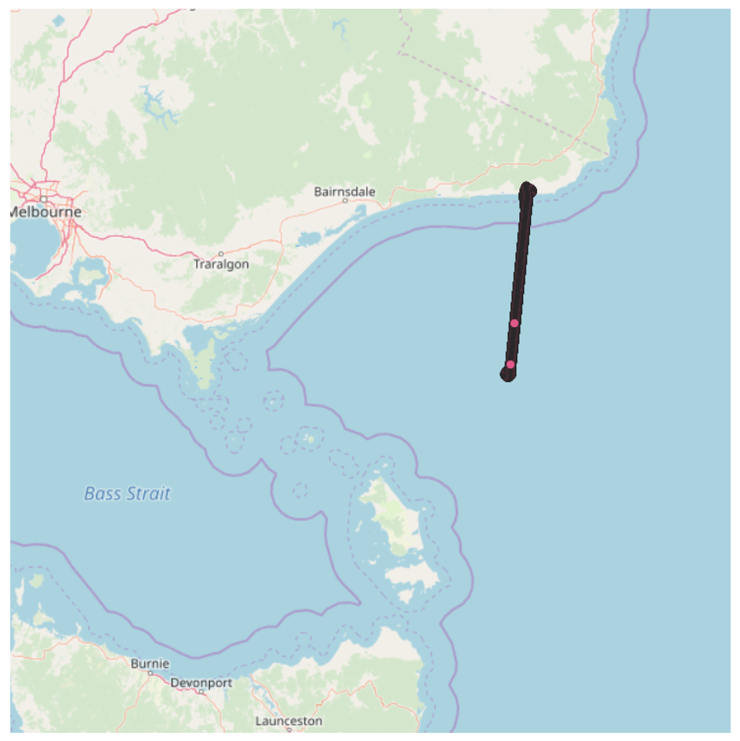
2. MIR Data Description

The data under analysis corresponds to a flight over the Bass Strait on 6 June 2018. The plane followed three passes over a straight line going from 37.9°S, 149.23°E to 38.9°S, 149.1°E, as shown in Figure 1. The GNSS-R data used include both L1/E1 and L5/E5a bands and also contain data from both GPS and Galileo constellations at different incidence angles and coming from different azimuths.

The plane flew at a height of $h\sim 1500$ meters at an average speed of 74 m/s. In that case, the specular reflection occurs in the first Fresnel zone, which is limited by the plane altitude by Equation (1),

$$\begin{array}{c}\hfill l_{Fr}={\displaystyle \frac{\sqrt{\lambda R_r}}{cos\left({\theta }_{inc}\right)}},where{R}_r={\displaystyle \frac{h}{cos\left({\theta }_{inc}\right)}}\end{array}$$

(1)

where $\lambda =19$ cm for L1, $\lambda =25$ cm for L5, $h=1500$ m, and ${\theta }_{inc}$ the wave incidence angle. Thus, at nadir ${\theta }_{inc}=0^{°}$ and $R_r=h$, which lead to a semi-major axis of the first Fresnel zone for L1 $l_{F{r}_{L1}}=17$ m, and for L5 $l_{F{r}_{L5}}=19$ m, and a Fresnel zone of $l_{F{r}_{L1}}=28$ m, and for L5 $l_{F{r}_{L5}}=33$ m for an incidence angle of ${\theta }_{inc}={45}^{°}$.

Considering the plane height and both L1 and L5 antenna 3 dB beam-width, ${\theta }_{L1}={18}^{°}$ and ${\theta }_{L5}={25.5}^{°}$, the footprint projection (in one direction) over the Earth surface is given by Equation (2),

$$L=R_r·\left(cotg\left({\theta }_{inc}-{\displaystyle \frac{{\theta }_{3dB}}{2}}\right)-cotg\left({\theta }_{inc}+{\displaystyle \frac{{\theta }_{3dB}}{2}}\right)\right)$$

(2)

where for an incidence angle ${\theta }_{inc}=0^{°}$ and ${\theta }_{3dB}={\theta }_{L1}$, L = 475 m, for a ${\theta }_{inc}=0^{°}$ and ${\theta }_{3dB}={\theta }_{L5}$ the coverage length is L = 678 m, for ${\theta }_{inc}={45}^{°}$ and ${\theta }_{3dB}={\theta }_{L1}$ the coverage length is L = 975 m, and for ${\theta }_{inc}={45}^{°}$ and ${\theta }_{3dB}={\theta }_{L5}$ the coverage length is L = 1430 m.

3. Coherency of the cGNSS-R Signal

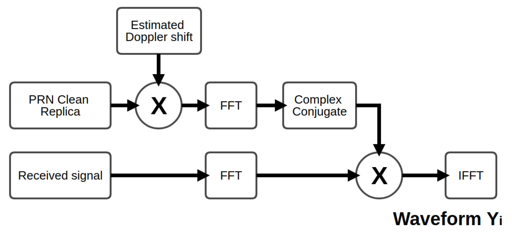
Conventional GNSS-R (cGNSS-R) is based on the correlation of the reflected signal $x\left(t\right)$ with a Doppler-shifted (v) clean replica of the GNSS code $y\left(t\right)$ [12]. In most GNSS-R instruments [13,14,15], the correlation time is limited by the code length used by the GNSS signal (i.e., ${\tau }_c=$ 1 ms for GPS L1 C/A, ${\tau }_c=$ 1 ms for GPS L5 without secondary codes, and ${\tau }_c=$ 20 ms for GPS L5 including secondary codes),

$$Y_i(\tau ,\nu )=\frac{1}{T_c}{\int }_{i{T}_c}^{(i+1)T_c}x\left(t\right)y^{*}(t-\tau )e^{-j2\pi \nu t}dt$$

(3)

There are several techniques used to perform this cross-correlation [16]: serial search, parallel phase search, or the most used in modern GNSS receivers, the parallel code-phase search (PCPS) algorithm. PCPS is based on the use of the Fast Fourier Transform (FFT) as large as 1 period of the code length (i.e., ${\tau }_c=$ 1 ms for GPS L1 C/A). Therefore, $Y_i$ is obtained as the Doppler cut containing the maximum absolute value of the signal.

In order to increase the signal-to-noise ratio (SNR), the resulting cross-correlation is incoherently averaged with subsequent correlations. The incoherent integration has been used for GNSS signal acquisition and also to perform DDMs, as it increases the observable SNR, but destroys the coherent part of the signal, which is the one coming from the specular reflection point, around the first Fresnel zone.

In [17], a method was proposed to detect and eliminate the direct signal. In this work, this technique is applied to detect the coherent component present in a GNSS-R signal. The technique explained in [17] consists of the computation of the variance of the coherently integrated DDM (Y in Equation (3)), i.e., prior to the incoherent averaging, as in Equation (4).

$$Var\left(Y\right)=E[{\left|Y\right|}^2]-{\left|E\left[Y\right]\right|}^2,$$

(4)

where $E[{\left|Y\right|}^2]$ is the incoherently averaged DDM. In practice, the variance term, $Var\left(Y\right)$ is computed as the mean square of the $N_{inc}$ samples (amount of samples incoherently averaged) minus the arithmetic mean of the samples ($\mu$), as in Equation (5). Note that Y is a complex value vectors, therefore any sum, multiplication, or mean calculus has to follow the complex arithmetic (i.e., mean of a complex vector is $mean\left(I\right)+j·mean\left(Q\right)$)

$$Var\left(Y\right)={\displaystyle \frac{1}{N_{inc}}}\sum _{i=1}^{N_{inc}}{\left|Y_i-\mu \right|}^2$$

(5)

$$\mu ={\displaystyle \frac{1}{N_{inc}}}\sum _{i=1}^{N_{inc}}{Y}_i$$

(6)

The difference of Equations (3) and (5) leads to the coherent component averaged over $N_{inc}$ samples, as shown in Equation (7).

$${\left|E\left[Y\right]\right|}^2={\displaystyle \frac{1}{N_{inc}}}\sum _{i=1}^{N_{inc}}{\left|Y_i\right|}^2-{\displaystyle \frac{1}{N_{inc}}}\sum _{i=1}^{N_{inc}}{\left|Y_i-\mu \right|}^2.$$

(7)

The implementation of the coherent integration as in Equation (7) opens many possibilities and analysis methods for signal processing. As an example, the ratio of both coherent component and total power waveform is defined as proposed in [18] as the degree of coherency (DOC), as in Equation (8). This ratio represents how coherent is the GNSS signal, for instance a direct GNSS signal has a DOC very close to 1. A reflected GNSS signal may have a large DOC in case of a quasi-specular reflection, but in general over land, it does not.

$$DOC={\displaystyle \frac{{\left|E\left[Y\right]\right|}^2}{E[{\left|Y\right|}^2]}}$$

(8)

4. Data Processing

The raw data is processed in different steps. First of all, each waveform $Y_i$ is used to perform both the coherent (7) and the variance calculations following the PCPS algorithm, as detailed in Figure 2. Note that, the PRN clean replica length, and therefore the final waveform length, is set by the PRN code length, which is 1 ms for GPS L1 C/A, 1 ms for the GPS L5 without secondary codes, and 20 ms for GPS L5 including the secondary codes.

The cross-correlation process is repeated $N_{inc}$ times for the amount of total integration time (both total power waveform and coherent component through the variance calculus), from now on, each of the $Y_i$ realizations will be identified as an integration period.

Once each $Y_i$ waveform for each of the $N_{inc}$ integration periods has been retrieved, the algorithm in Figure 3 is followed in order to provide the three products: total power waveform; variance part (which is the incoherent part); its difference, which corresponds to the coherent component of the signal; and finally the phase evolution for each integration period.

Note that, mean() and var() functions are calculated over Yi, where $i=1$ to N, and N is the integration time.

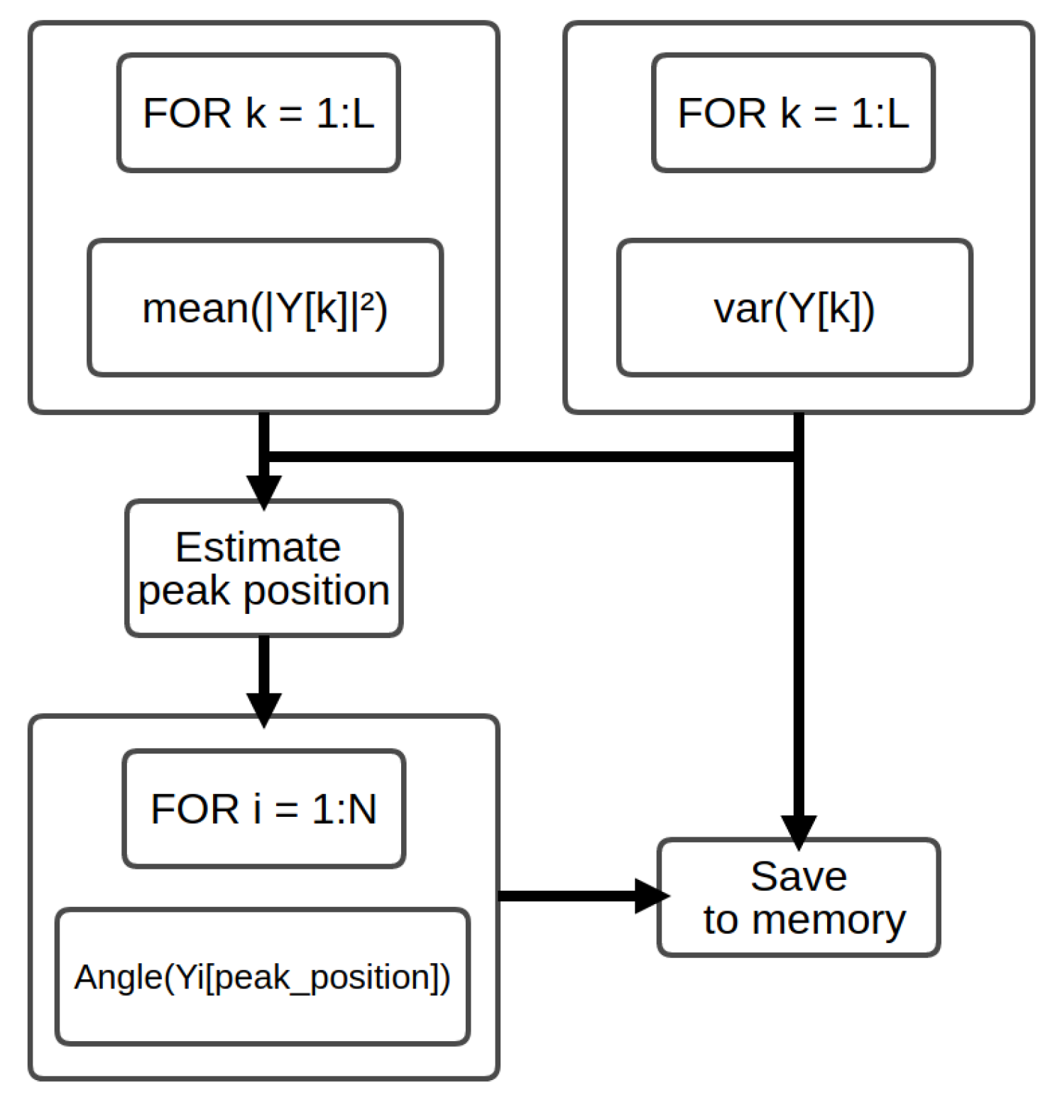
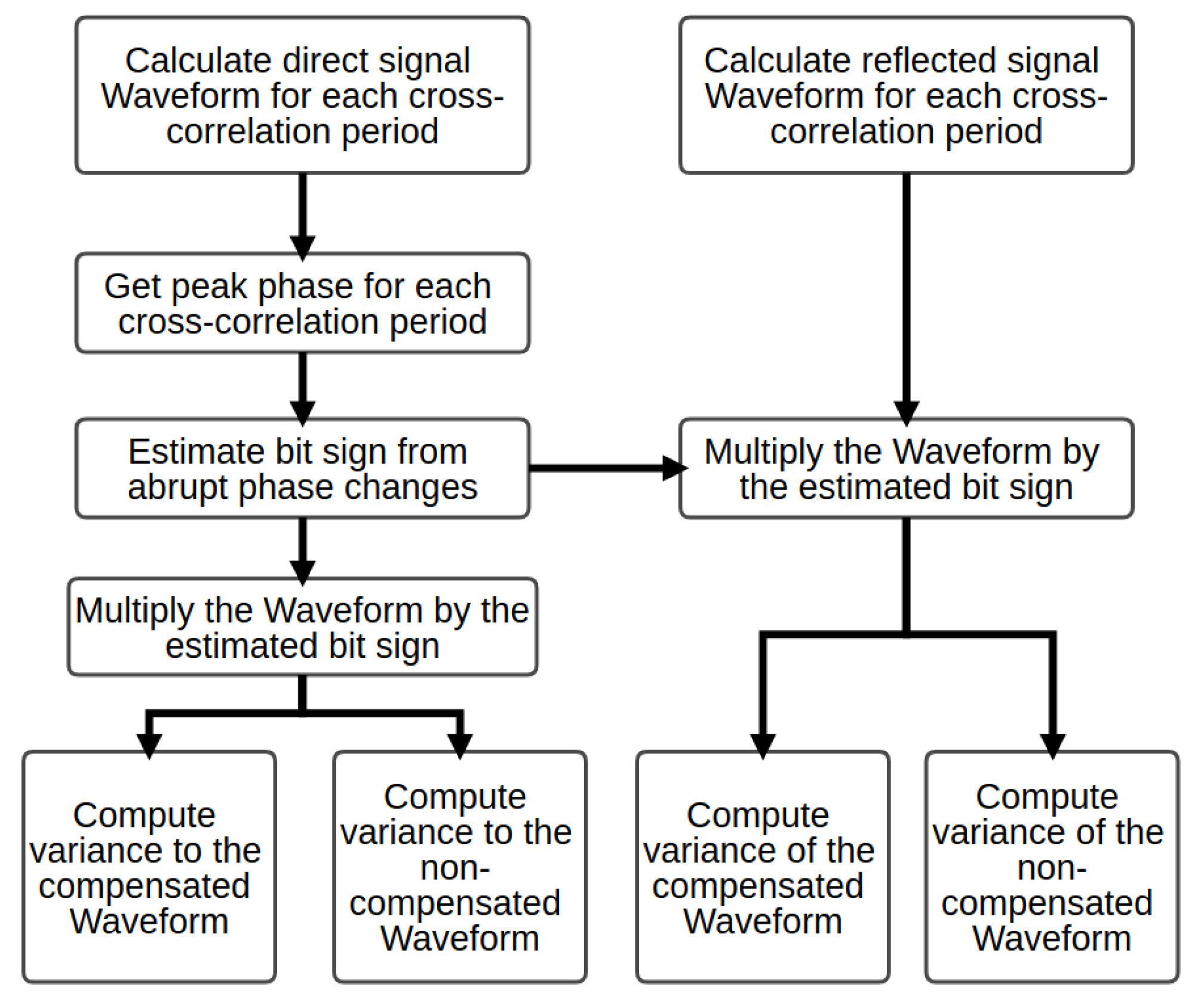
4.1. Navigation Bit Transitions during the Coherent Integration

As described in [19], the bit transition in GNSS needs to be handled in case of large coherent integration periods. The variance method is also sensitive to the bit change, therefore a bit change in the middle of the integration process causes that the coherent term in Equation (5) drops to zero. The bit transition effect can be compensated by means of retrieving the navigation bit sign and multiplying each of the resulting waveforms ($Y_i$), by the corresponding sign. The navigation bit sign is retrieved by looking at the phase evolution during the integration period.

The Navigation bit transition can also affect the reflected GNSS signal in case the coherency is preserved in the reflection. However, this is not actually the case, and thus the navigation bit cannot be retrieved and compensated as easy as in the direct signal case. In such cases, the navigation bit can be compensated using the direct signal information. The algorithm to retrieve the coherent part for both direct and reflected signals, compensating the navigation bit transition, is detailed in Figure 4.

In order to estimate the bit sign ($\widehat{x}$) in the direct signal, the discriminator in Equation (9) is used.

$$\widehat{x}=atan2\left(Q,I\right),$$

(9)

where Q is the imaginary component of the WAF ($Y_i$) at its peak (for both code and Doppler), I the real component, and atan2 is the four quadrant arctangent function.

4.2. Open-Loop Tracking of the Coherent Part of the Reflected Signal

The described algorithm allows for an open-loop tracking of the reflected signal with a variable coherent integration time compensating the bit transitions because of the information of the direct signal. In addition, this algorithm stores both the bit-compensated and the non-compensated coherent integrated waveforms, which are useful to evaluate the coherency characteristics of the signal (i.e., the reflected signal can contain a coherent part, but no bit information can be retrieved).

Figure 5 illustrates the bit change effect on the impact on the coherency part in a GPS L1 C/A GNSS signal captured by the MIR instrument and integrated during 40 ms. A data set containing two bit transitions (periods 12 and 32 as seen in the phase plot) in the middle of the integration has been selected. As seen, the coherent part in case the non-compensated case (dash-dot black line) for the direct signal goes down to zero, as the coherency is lost due to the navigation bit change. However, as the bit transition is detected and compensated, the coherent (dashed blue line) part goes almost as high as the total power waveform; therefore, the direct signal DOC for this example is ∼0.9.

The reflected case is quite different. First of all, as expected, the coherency of the signal is much lower than the direct one, but also the navigation bit compensation does not make any difference in terms of the coherency. Note that the phase evolution in the reflected peak presents the 180° jump at the 12th integration period, but after the 22nd period, it completely losses the phase and hence the coherency of the signal. Despite that, the signal presents a coherent component with a DOC ∼0.2.

Note that in the case of reducing the integration time to 20 ms, to avoid the signal coherency degradation present at the 22nd period, the DOC of the reflected signal increases (as shown in Figure 6) up to ∼0.8, as expected. Therefore, this increase on the DOC for 20 ms of integration that the reflection is almost coherent in this period.

4.3. Coherency in the Presence of Secondary Codes

The secondary codes present in GPS L5 signal produce a similar behavior on the coherent part than the navigation bit. As the navigation information, the secondary code is a pseudorandom sequence of +/−1, thus multiple sign changes occur in a 1 ms integration period. As the repetition period of the secondary code for GPS L5 is 20 ms, performing the coherent integration as in GPS L1 C/A without the secondary code produces a degradation on both direct and reflected signals, as shown in Figure 7, with a DOC for both direct and reflected <0.05. Note that the integration has been performed over the pilot component, as in that way we are able to remove the entropy of the navigation bit sign change.

However, performing the cross-correlation, but now including the secondary code, and preserving the integration time (40 ms) has a direct impact on the DOC. As seen in Figure 8, the DOC of both direct and reflected signal goes up to ∼1, which means that, for the selected waveform, the coherency of the sea spectrum at L5 is preserved within 40 ms. Note as well the typical elongation of the trailing edge of the waveform (Figure 7, central panel), and that, in the reflected signal case, two coherent peaks can be identified. In addition, the phase evolution of the L5Q signal with secondary codes included can only be represented once every 20 ms, as the cross-correlation process and waveform retrieval is taken in multiples of the code length.

The second reflection peak seen in this figure is placed seven samples away from the first peak. Converting the sample distance to meters (as in Equation (10)), we clearly see that this second peak is out of the first Fresnel zone (27 m for L5); therefore, it came from the reflection glistening zone, but presenting a coherent component.

$$\begin{array}{c}\hfill {\Delta }_m=c·{\displaystyle \frac{{\Delta }_{samples}}{f_s}}\\ \hfill {\Delta }_m=64m\end{array}$$

(10)

where c is the light speed, $f_s$ = 32.768 MHz is the sampling rate, and ${\Delta }_{samples}$ corresponds to the peak-to-peak distance in samples.

5. Reflected Signal Coherency Analysis

This section covers an analysis of different GPS L1 and L5 signals for different integration times.

As seen in Equation (10) in [20] the coherency time of a given surface for this flight is for both L1 and L5, and assuming an incidence angle of 0° and 45°.

$$\begin{array}{c}\hfill {\tau }_s=\frac{\lambda }{2·v}\sqrt{\frac{h}{2·c·{\tau }_c·cos\left({\theta }_i\right)}},\\ \hfill {\tau }_{s_{L1}}({\theta }_{inc}=0^{°})=2ms,{\tau }_{s_{L1}}({\theta }_{inc}={45}^{°})=2.8ms,\\ \hfill {\tau }_{s_{L5}}({\theta }_{inc}=0^{°})=7.7ms,{\tau }_{s_{L5}}({\theta }_{inc}={45}^{°})=10ms\end{array}$$

(11)

This section analyzes a set of different waveforms for GPS L1 C/A and GPS L5Q with secondary codes. Those waveforms have been selected and reproduced for a set of integration times, which are multiples (up to 10 times) of the sea coherence time. In addition, the analysis does not only cover the waveform shape, but the phase of the signal at all the integration steps, which helps to understand why the signal has a given coherency or not.

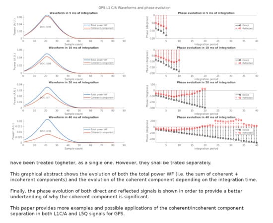
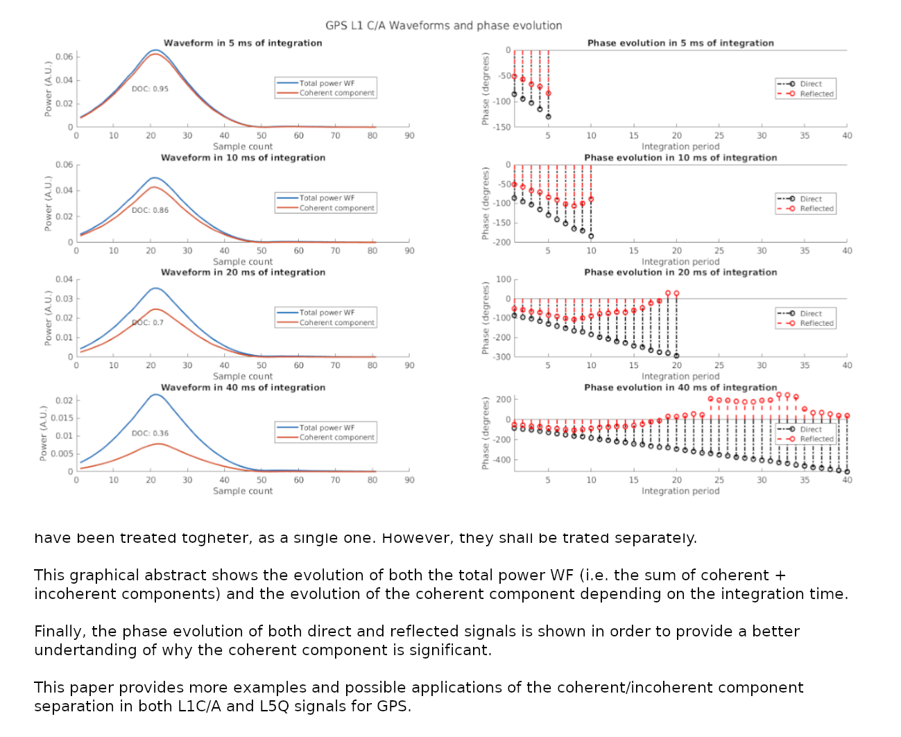
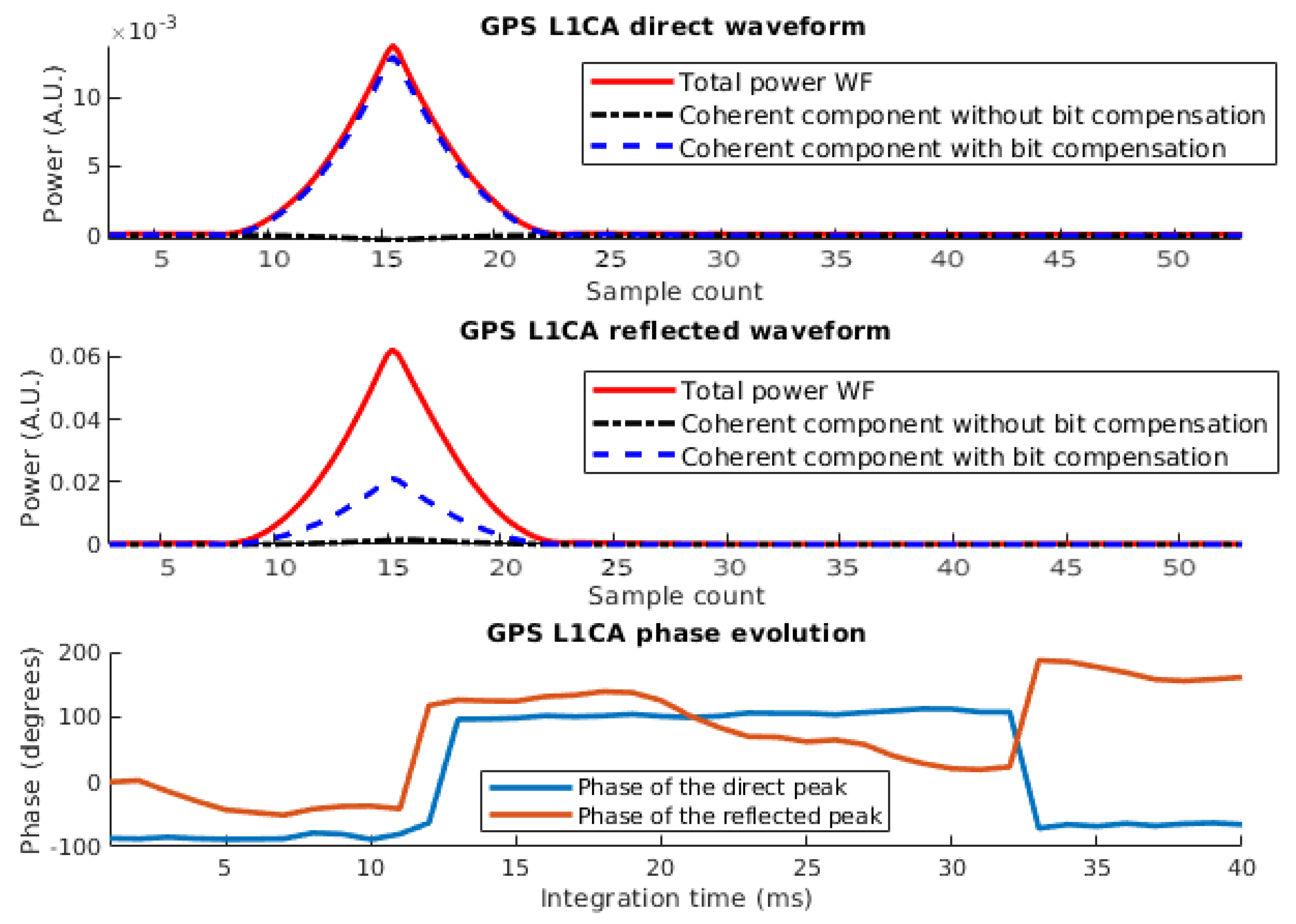
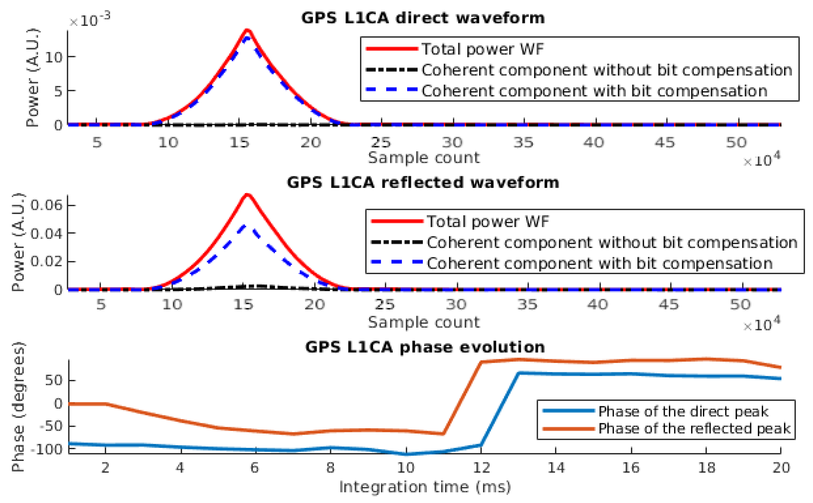
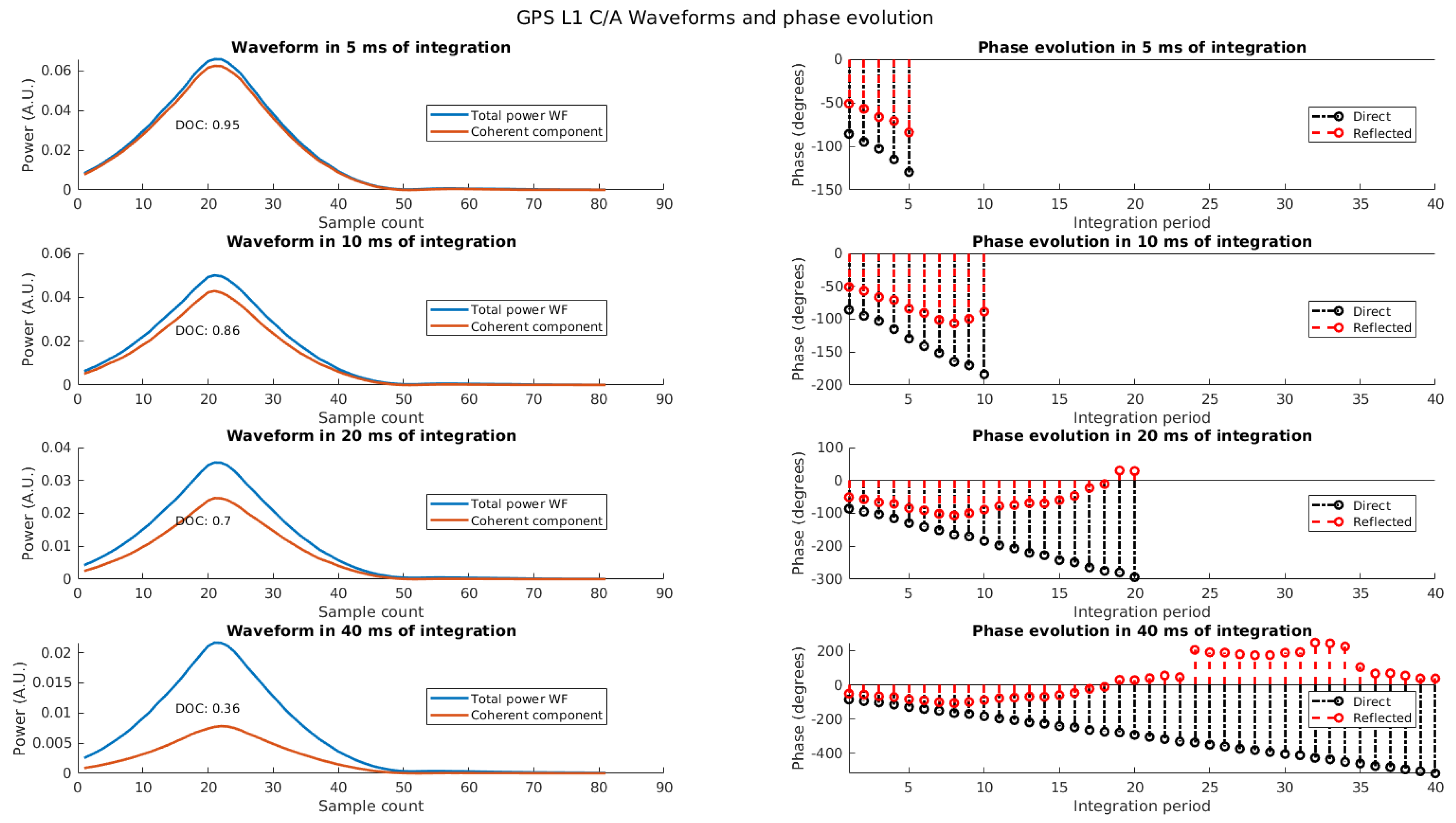
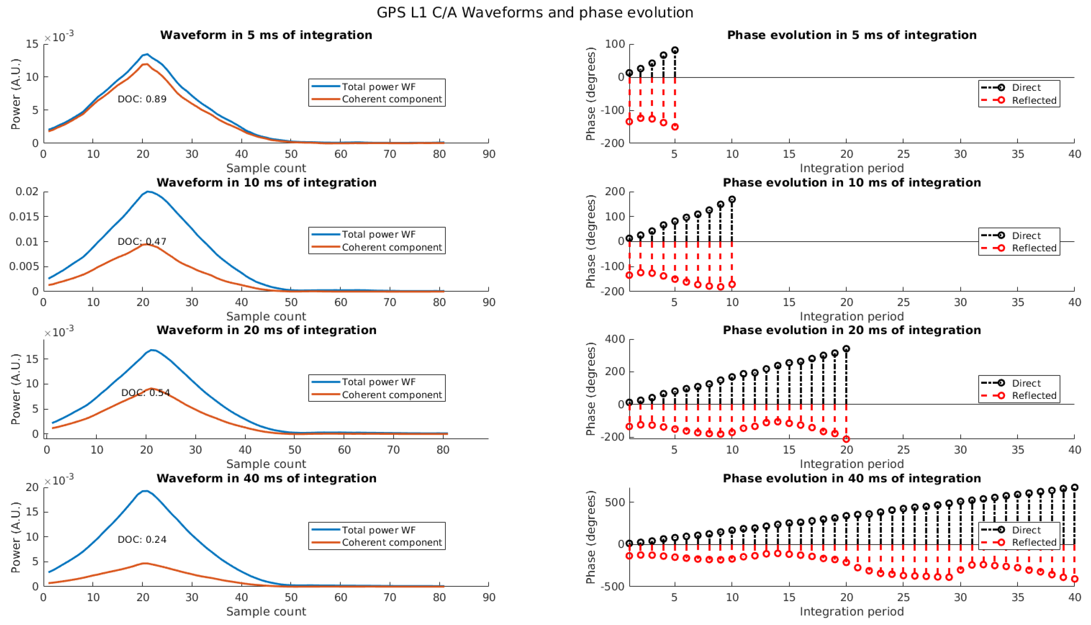
5.1. GPS L1 C/A Reflected Signal Signatures

The GNSS reflected signal contains a portion of coherency, which is easily untangled from the incoherent one thanks to the proposed algorithm. A first example for GPS L1 C/A is provided in Figure 9 showing four different integration times: 5 ms, 10 ms, 20 ms, and 40 ms. As it can be seen, the DOC of the reflected waveform decreases as the coherent integration time increases. In addition, the phase of the peak is detailed for each 1 ms cross-correlation interval. Note that, the scale of the phase evolution has been set the same for the four measurements to ease its visualization.

Note that, the phase for the direct signal is flat and does not present 180° jumps, as the navigation bit has the same sign for the 40 ms. Note also that the phase unwrapping function has been used to ease the visualization of the phase evolution.

Analyzing the DOC for the four cases, the DOC decreases as the integration time increases, which is logical due to the coherence time of the sea as shown in Equation (11).

In addition, analyzing the phase variation for the four cases (and in particular the 20 and 40 ms case), the coherency loss is coming from a change of the reflected surface, as, for instance, the reflection has gone from the wave crest to the wave valley. As seen, the peak phase is very smooth and follows a shape which can be identified as the wave evolution with time. This was first observed in a controlled experiment in a water tank (Figures 7 and 10 of [21]). This phase precision can be actually used to perform phase altimetry measurements as in [22,23].

The second example (Figure 10) shows a noisier environment, where the coherency of the signal is almost lost after 10 ms of integration. As seen in the 10 ms and 20 ms examples, the phase evolution of the reflected signal is very noisy, which causes a coherence loss. However, despite the phase is not constant in this case, the coherent component can be still untangled from the incoherent one, allowing for that a better estimation of the first Fresnel zone characteristics and the surface roughness associated to the illuminated area.

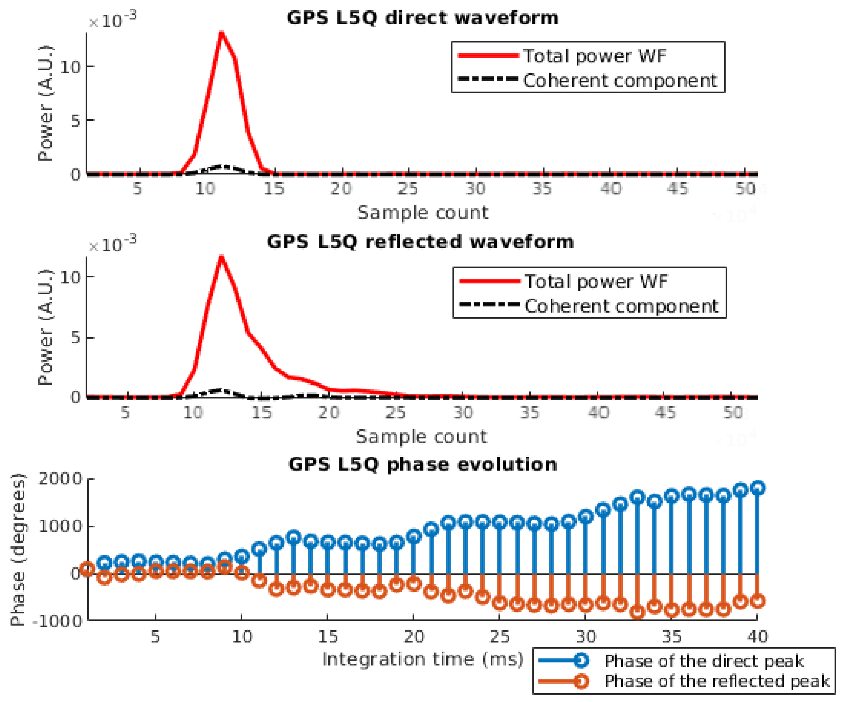
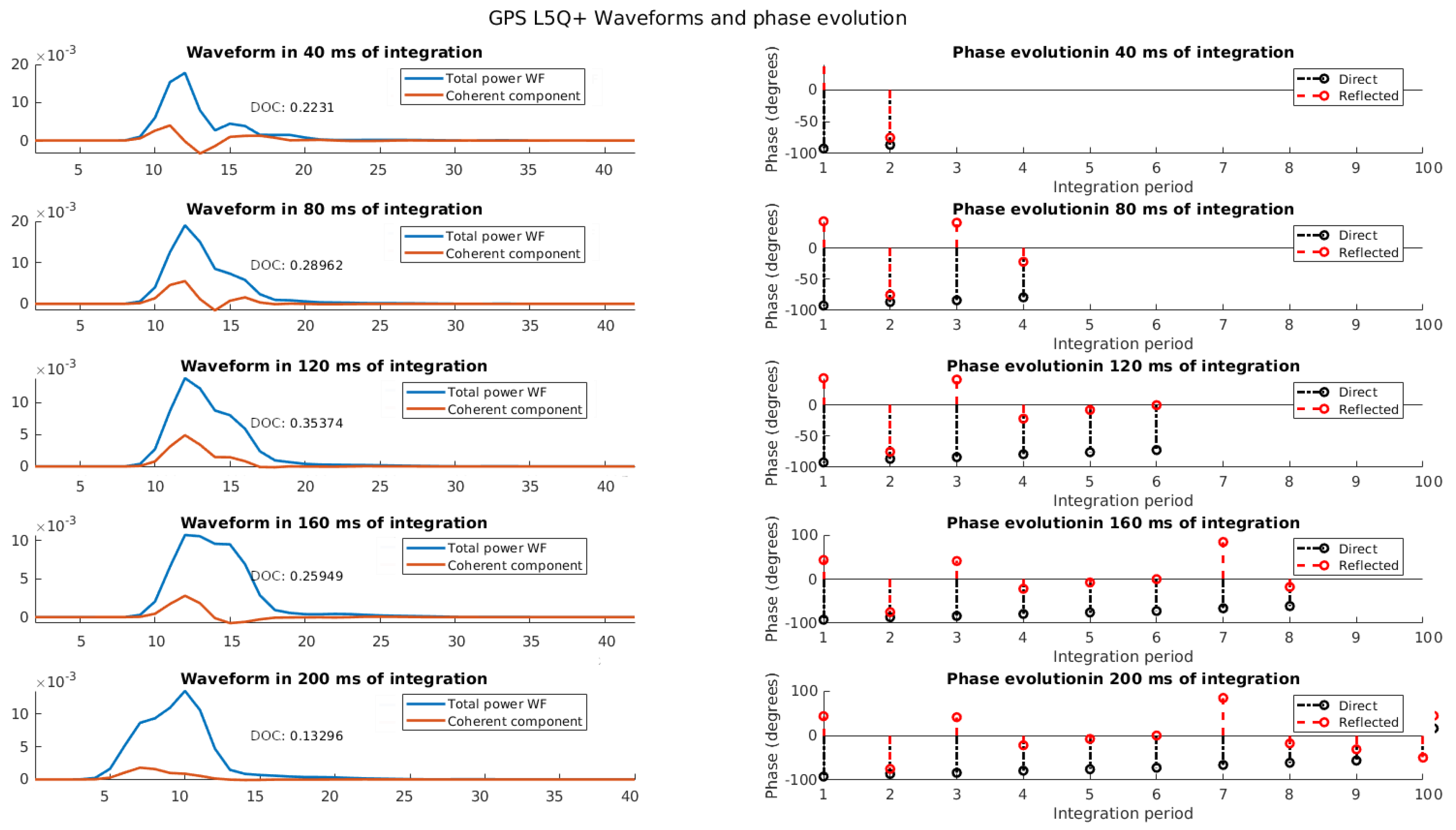
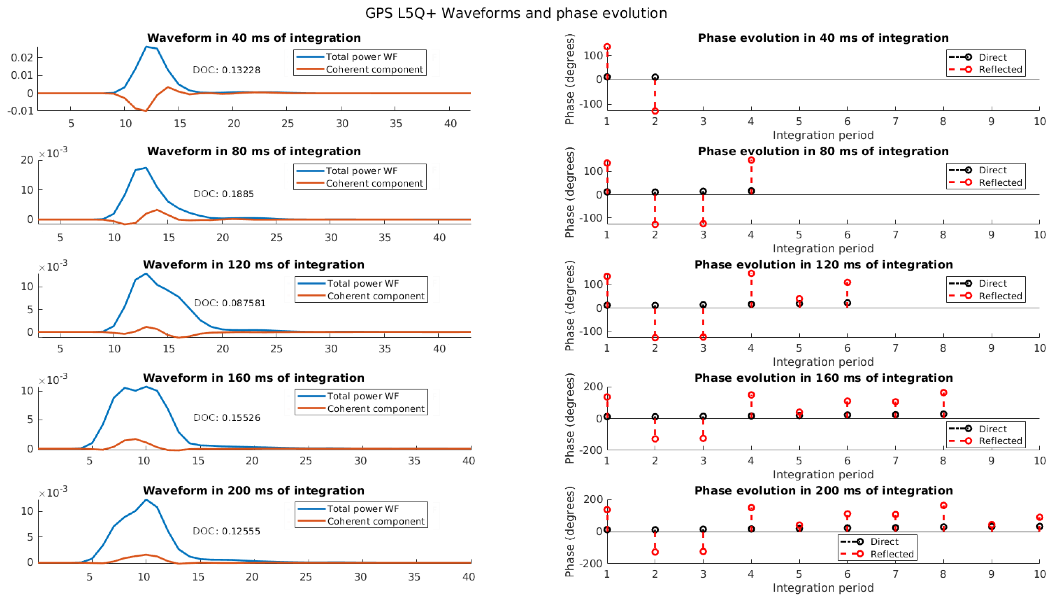
5.2. GPS L5Q Reflected Signal Signatures

As presented in Section 4.3, the coherency of the L5 signal (either I or Q components) is lost if the secondary codes are not taken into account. Two examples for GPS L5Q with secondary codes are provided for five different integration time: 40 ms, 80 ms, 120 ms, 160 ms, and 200 ms.

The first example is shown in Figure 11. In the 40 ms case of this figure, it is seen that the coherent component presents a positive and a negative part, as it is a real correlation and the coherent integration is not based on the absolute value operation. This negative part can be identified as an out-of-phase addition of the reflected signal paths. Despite that, the signal presents a high coherency, with a DOC ∼0.22 for 40 ms of integration. In addition, the coherent peak due to the incoherent integration is not located in exactly the same chip delay than the incoherent one. The position of this coherent peak is also very useful for altimetry applications, as, from one side, the coherent reflection is linked only to the first Fresnel zone (i.e., better spatial resolution), and from the other side, the peak position estimation is better than in the incoherent case.

As seen in the 80, 120, 160, and 200 ms cases, increasing the integration time also increases the blurring of the total power waveform (no retracking applied [24]), also providing evidence that the peak position for the total power case is changing. Despite that, the coherent peak is not moving from its original position, as it is only identifying the coherent reflection, and not all the contributions from the glistening zone. Even though the coherent component is still, its amplitude decreases as the integration time increases due to the surface changes among time. Take into account that, after 200 ms, the plane has been moved ∼15 m, which is half of the the first Fresnel zone size at L5.

In addition to the waveform analysis, the phase evolution and its difference with respect to the direct signal one gives very useful information. The difference between both is changing as the integration time increases. In this case, the direct phase is still, and the reflected phase changes within $\pm {100}^{°}$. The abrupt changes in phase is indicating two different phenomena: on one hand, the signal coherency is not 100% preserved between one integration step and the next one, which is also reflected in the DOC parameter. On the other hand, the phase evolution follows a half-sine slope, which may be linked with the sea surface shape at the specular point. Therefore, further processing this phase evolution, taking into account the peak position enhancement thanks to the coherent integration will help to enhance phase altimetry precision [23].

Finally, the second example for L5Q shows a very different shape as the previous example. As seen in Figure 12, the larger the integration time, the larger the change of the shape of the coherent component. First of all, the DOC for the 5 cases is very similar, on the order of $\sim 0.1$, which means that even a small coherency is preserved for even large integration times.

The first case (40 ms of integration) shows a first negative peak on the coherent part, followed by a positive peak. Comparing it to the total power waveform, which uses the modulus operator, the presence of this negative peak tells us that the specular reflection (and hence the coherent one) is coming from the positive coherent component, which is two lags away from the peak estimation of the total one.

Looking at the evolution of both the coherent and total power peak positions with respect to the integration time, it is clear that as the total one gets blurred and its maximum moves within 20 samples, the coherent one is almost frozen at the same sample, and starts blurring when the integration time is too large. Looking at the phase evolution for this example, it is clear that the coherency of the signal is not high, as the phase performs ∼180° jumps from one integration period to the next one, while the direct phase is the same. In this case, a half-sine shape can be identified for large integration times, which can be linked to the sea slope, and hence indicating that phase altimetry may be feasible and will be enhanced thanks to the coherent component peak position determination.

6. Potential Applications from the Coherent Component Analysis of the GNSS-R Waveform

The previous sections have shown that the coherent component of the GPS L1 C/A and GPS L5, including secondary codes, is not negligible. This component decreases as the integration time increases, and its decreasing ratio depends on the roughness of the reflected surface, as it is linked to the surface coherence time. The application of the coherent component untangling technique opens a number of potential applications from its use, which are highlighted below.

6.1. Scatterometry Using the Coherent Component

As seen from the GPS L1 C/A case, the coherent component is very strong for short integration times. In addition, knowing that the coherent component reflection comes from the specular point, scatterometry measurements are much easier to compute and also with a better spatial resolution.

From now, the scattering model used to compute scatterometry measurements assumes a normalized bistatic scattering cross section (${\sigma }_0$) over the full glistening zone of the reflected surface [25]. In this case, the reflected area is very large, therefore having a poor spatial resolution. However, as the coherent component contains the reflection from the specular point, and hence the first Fresnel zone, the spatial resolution of the reflected signal is improved. At this point, scatterometry measurements are as easy as computing the power ratio between the direct and the reflected signal coherent components, as in Equation (12).

$$\begin{array}{c}\hfill \Gamma ={\displaystyle \frac{P_{ref}}{P_{dir}}}={\left({\displaystyle \frac{R_{T-SP}+R_{SP-R}}{R_{T-R}}}\right)}^2·{\displaystyle \frac{G_{zenith}({\theta }_{dir},{\varphi }_{dir})}{G_{nadir}({\theta }_{ref},{\varphi }_{ref})}}·{\displaystyle \frac{G_T({\theta }_1,{\varphi }_1)}{G_T({\theta }_2,{\varphi }_2)}}\end{array}$$

(12)

where $R_{T-SP}$, $R_{SP-R}$, and $R_{T-R}$ are the distances from the transmitter to the specular reflection point, from the specular reflection point to the receiver, and from the transmitter to the receiver, respectively; $G_{zenith}$ and $G_{nadir}$ are the gain of the receiver antennas; and $G_T$ is the gain of the transmitter antenna in the direction of the specular point and the receiver position. Note that the $G_T$ term can be neglected for receivers and specular points that are very close (i.e., the specular point is almost at nadir), or for low altitude receivers (i.e., a plane flying at 1500 meters height). In addition, the range correction term is ≃1 and can be neglected for low altitude platforms, but it can be a fraction of a dB for LEO satellites.

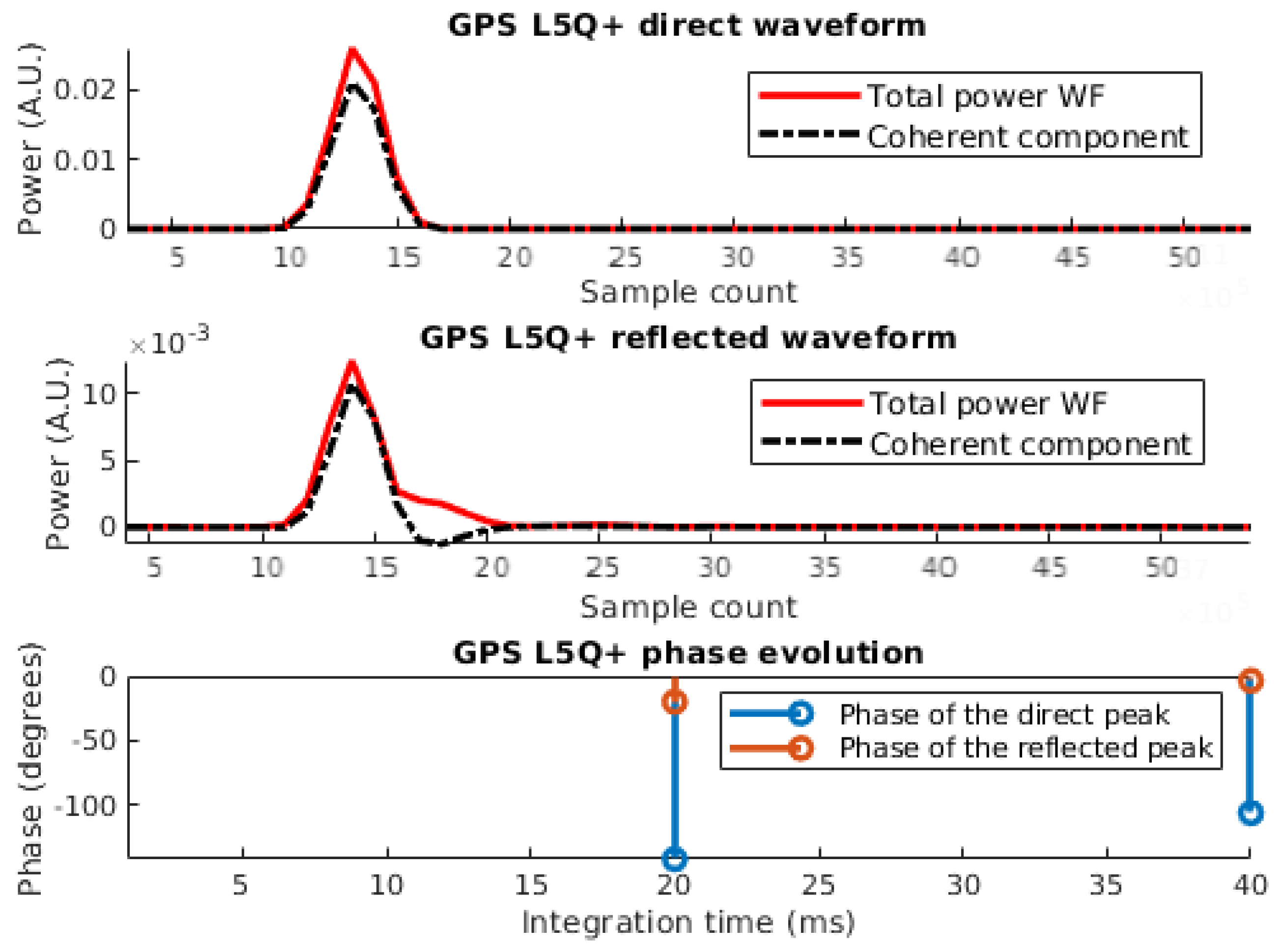
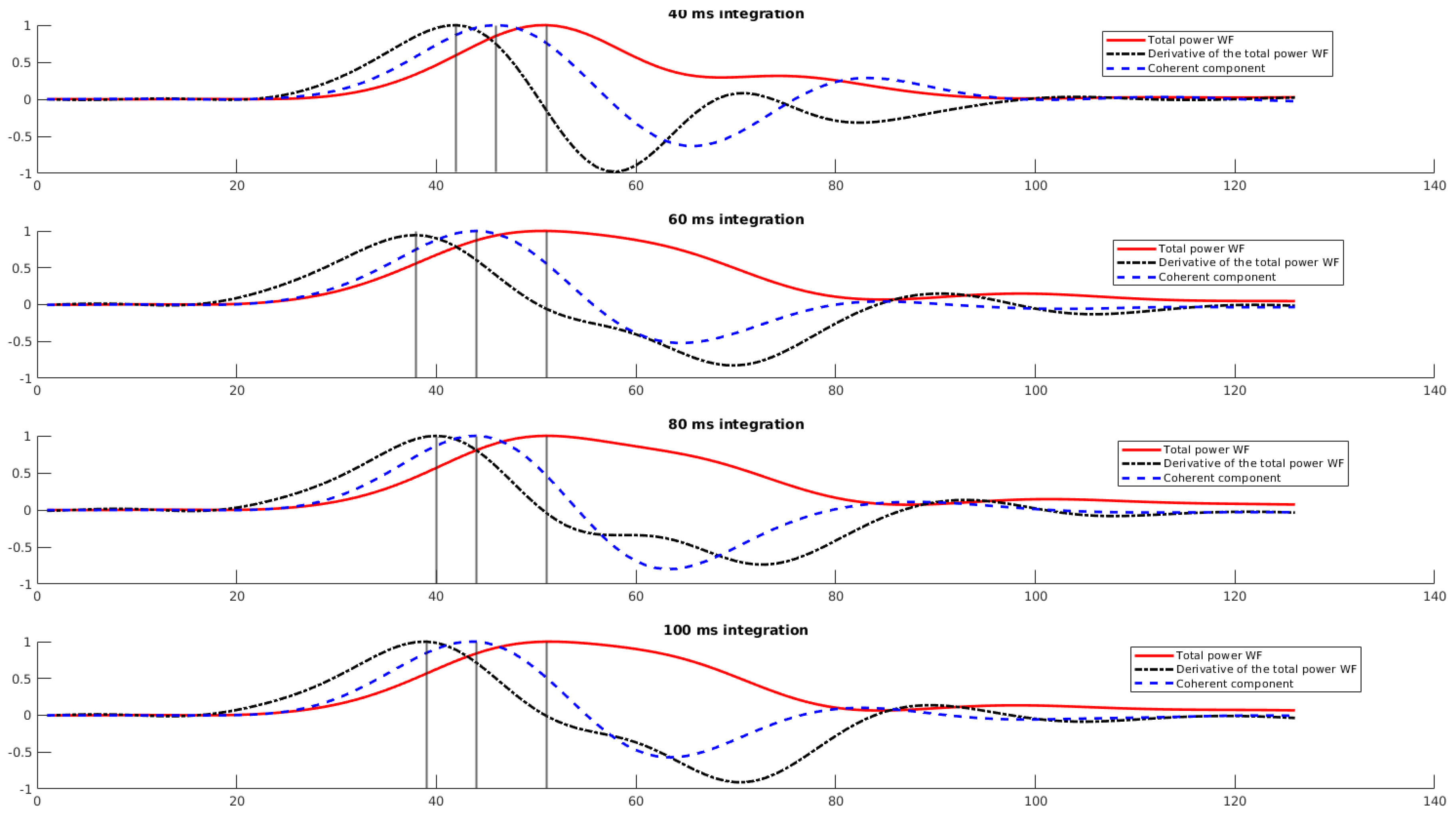
6.2. Precise Altimetry from Precise Peak Position Estimation in L5Q+ Waveforms

From the examples provided in Section 5.2, it is clear that the coherent part of the GNSS L5Q signal with secondary codes provides additional information of the peak position, which can be useful to estimate the lag corresponding to the maximum position of the waveform. The better the estimation of this peak, the better the altimetry resolution. The example shown in Figure 13 is a zoom of a L5Q+ reflected waveform. Both total power and coherent parts of the reflected signal have been interpolated by 8 (i.e., $f_s=262.144$ MHz) using the FFT interpolation method. In addition, the derivative of the total power part is calculated. Note that all three signals have been normalized with respect to its maximum value in order to ease its visualization.

For the four cases, 40, 60, 80, and 100 ms of integration time, the coherent component peak position is found in five samples for the 40 ms case, and seven samples for the next three cases before the peak of the total power averaged.

In addition, the peak of the coherent component is placed between 9 and 13 samples after the maximum of the derivative of the total power waveform, which means that the actual specular point (in terms of lag delay) is placed between the point of maximum slope of the total power waveform and the actual maximum of the waveform. This behavior was studied in [26], which for an ideal conditions of a rough surface, and a theoretically infinite incoherent integration time, the delay corresponding to the specular point was placed right on the maximum of the derivative of the total power waveform. In the example shown in this study, the delay corresponding to the specular point is identified as the coherent component peak.

A proper estimation of the specular reflection point gives an improved accuracy of the altimetry measurement, as seven samples of difference in the estimation of this peak leads to an error up to 3 m (i.e., for an incidence angle of 45°, from Equation (34) in [12]).

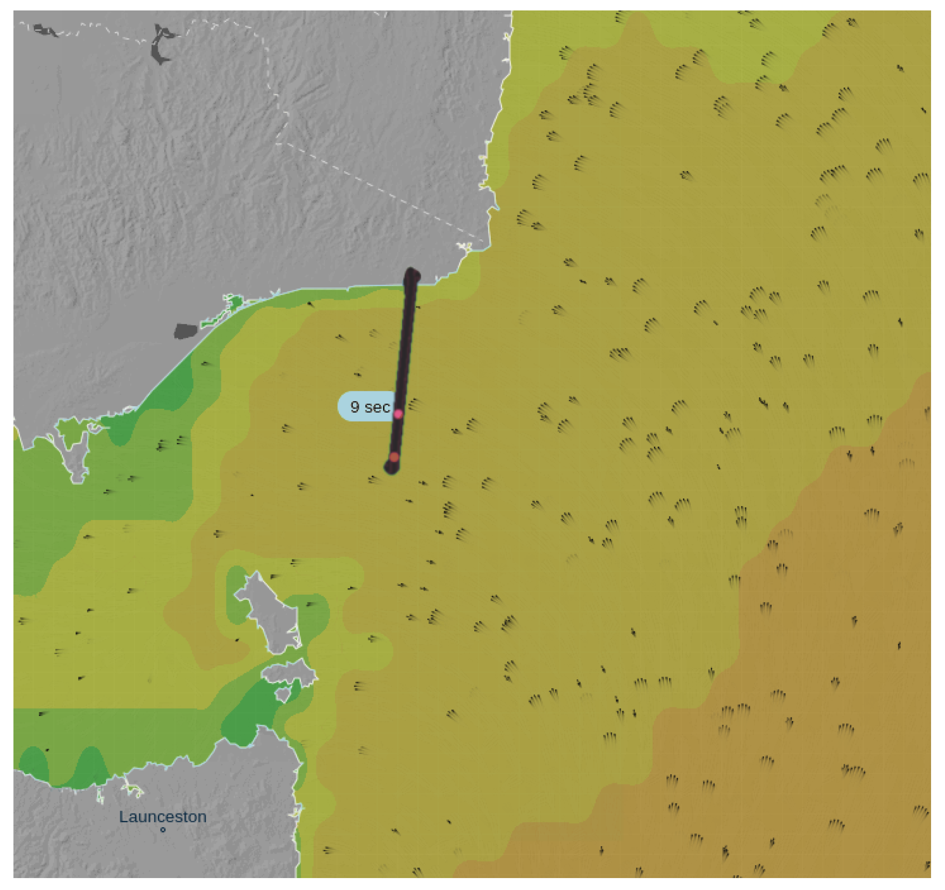
Swell Wave Period from Secondary Peaks in L5Q+ Waveforms

As seen in Figure 13, apart from the waveform peak, there are several secondary peaks, mainly in the 40 ms of integration case, whose second reflection is identified in both coherent component and total power processed reflected waveforms. The 60, 80, and 100 ms cases present a secondary peak in the coherent component, but not in the total one. Despite the incoherent integration has blurred up the waveform for relative large integration times, the coherent component presents the same secondary peak, indicating that the incoherent integration is preventing other applications of the GNSS-R. Note that the secondary peaks that are always positive in the total power waveform, are negative in the coherent one, but still it represents a coherent reflection with negative sign (i.e., 180° rotation with respect to the specular peak).

Taking as a reference the coherent component maximum, the first secondary peaks (i.e., the negative ones) are placed ∼20 samples away from the maximum one. Transforming the sample distance to meters following Equation (10) but with $f_s=262.144$ MHz, the ${\Delta }_m$ is ∼23 m. Moving to the third, which is almost negligible in the figure, it is placed ∼37 samples from the maximum, therefore giving a ${\Delta }_m$∼42 m.

Looking to the sea state conditions during the flight in [27] (see Figure 14), it is found that swell waves had a period of $T_{waves}$∼9 s, which corresponds to a sea speed ($C_{waves}$) and a wavelength (i.e., distance between crests) as in Equation (13) of [28].

$$\begin{array}{c}\hfill C_{waves}=1.56·T_{waves}\simeq 14m/s,\\ \hfill {\mathsf{\Lambda }}_{waves}=C_{waves}·T_{waves}\simeq 126m.\end{array}$$

(13)

In the exposed case, the maximum distance found is ∼57 m, which is approximately $\frac{{\mathsf{\Lambda }}_{waves}}{2}$. This distance corresponds to a two reflections on consecutive wave crests. Therefore, the negative coherent peak corresponds to the sum of the components reflected between the wave crest and the wave trough.

7. Conclusions

This study has presented a technique to untangle the coherent signal from the total power waveform on reflected GNSS signals from the sea surface, for both L1 and L5 bands from GPS. The results presented confirm the presence of a non-negligible coherent component in a reflection over the sea surface from an aircraft at 1500 m height.

A waveform and phase evolution analysis has been presented, allowing the processing of the coherent and total power components separately. The application of this technique to any GNSS-R signal opens new possible applications. Including a better resolution for altimetry products thanks to a better estimation of the peak position, the estimation of the wave period thanks to the identification of the secondary peaks present on the coherent component, and other derived products such as the sea state ($U_{10}$), and the sea surface height with improved resolution.

Finally, the combination of both precise altimetry measurements and secondary peak identification can provide a more complete analysis of the sea state, not only the swell period, but also the swell amplitude.

References

1. Voronovich, A.G.; Zavorotny, V.U. The Transition From Weak to Strong Diffuse Radar Bistatic Scattering From Rough Ocean Surface. IEEE Trans. Antennas Propag. 2017, 65, 6029–6034. [Google Scholar] [CrossRef]
2. Carreno-Luengo, H.; Camps, A. Unified GNSS-R formulation including coherent and incoherent scattering components. In Proceedings of the 2016 IEEE International Geoscience and Remote Sensing Symposium (IGARSS), Beijing, China, 10–15 July 2016. [Google Scholar] [CrossRef]
3. Camps, A. Spatial Resolution in GNSS-R Under Coherent Scattering. IEEE Geosci. Remote Sens. Lett. 2020, 17, 32–36. [Google Scholar] [CrossRef]
4. Alonso-Arroyo, A.; Zavorotny, V.; Camps, A. Sea Ice Detection Using U.K. TDS-1 GNSS-R Data. IEEE Trans. Geosci. Remote Sens. 2017, 55, 4989–5001. [Google Scholar] [CrossRef] [Green Version]
5. Alonso-Arroyo, A.; Camps, A.; Park, H.; Pascual, D.; Onrubia, R.; Martin, F. Retrieval of Significant Wave Height and Mean Sea Surface Level Using the GNSS-R Interference Pattern Technique: Results From a Three-Month Field Campaign. IEEE Trans. Geosci. Remote Sens. 2015, 53, 3198–3209. [Google Scholar] [CrossRef] [Green Version]
6. Rodriguez Alvarez, N.; Camps, A.; Vall-llossera, M.; Bosch, X.; Monerris, A.; Ramos-Perez, I.; Valencia, E.; Marchan, J.; Martínez-Fernández, J.; Baroncini Turricchia, G.; et al. Land Geophysical Parameters Retrieval Using the Interference Pattern GNSS-R Technique. IEEE Trans. Geosci. Remote Sens. 2011, 49, 71–84. [Google Scholar] [CrossRef]
7. Carreno-Luengo, H.; Amézaga, A.; Vidal, D.; Olivé, R.; Martin, J.M.; Camps, A. First Polarimetric GNSS-R Measurements from a Stratospheric Flight over Boreal Forests. Remote Sens. 2015, 7, 13120–13138. [Google Scholar] [CrossRef] [Green Version]
8. Gerlein-Safdi, C.; Ruf, C.S. A CYGNSS-Based Algorithm for the Detection of Inland Waterbodies. Geophys. Res. Lett. 2019, 46, 12065–12072. [Google Scholar] [CrossRef]
9. Onrubia, R.; Pascual, D.; Park, H.; Camps, A.; Rüdiger, C.; Walker, J.; Monerris, A. Satellite Cross-Talk Impact Analysis in Airborne Interferometric Global Navigation Satellite System-Reflectometry with the Microwave Interferometric Reflectometer. Remote Sens. 2019, 11, 1120. [Google Scholar] [CrossRef] [Green Version]
10. Pascual, D.; Onrubia, R.; Alonso-Arroyo, A.; Park, H.; Camps, A. The microwave interferometric reflectometer. Part II: Back-end and processor descriptions. In Proceedings of the International Geoscience and Remote Sensing Symposium (IGARSS), Quebec City, QC, Canada, 13–18 July 2014; pp. 3782–3785. [Google Scholar] [CrossRef]
11. Valencia, E.; Camps, A.; Marchan-Hernandez, J.F.; Bosch-Lluis, X.; Rodriguez-Alvarez, N.; Ramos-Perez, I. Advanced architectures for real-time Delay-Doppler Map GNSS-reflectometers: The GPS reflectometer instrument for PAU (griPAU). Adv. Space Res. 2010, 46, 196–207. [Google Scholar] [CrossRef]
12. Zavorotny, V.U.; Gleason, S.; Cardellach, E.; Camps, A. Tutorial on Remote Sensing Using GNSS Bistatic Radar of Opportunity. IEEE Geosci. Remote Sens. Mag. 2014, 2, 8–45. [Google Scholar] [CrossRef] [Green Version]
13. Jales, P. Spaceborne Receiver Design for Scatterometric GNSS Reflectometry. Ph.D. Thesis, University of Surrey, Guildford, UK, 2012. [Google Scholar]
14. eoPortal Directory. Cyclone GNSS Mission Description Website. Available online: https://directory.eoportal.org/web/eoportal/satellite-missions/c-missions/cygnss (accessed on 2 January 2019).
15. Munoz-Martin, J.F.; Fernandez, L.; Ruiz-de-Azua, J.; Camps, A. The Flexible Microwave Payload -2: A combined GNSS-R and L-band radiometer with RFI mitigation payload for CubeSat-based Earth Observation Missions. In Proceedings of the 2019 IEEE International Geoscience and Remote Sensing Symposium (IGARSS), Yokohama, Japan, 28 July–2 August 2019. [Google Scholar]
16. Khan, R.; Khan, S.U.; Zaheer, R.; Khan, S. Acquisition strategies of GNSS receiver. In Proceedings of the International Conference on Computer Networks and Information Technology, Abbottabad, Pakistan, 11–13 July 2011; pp. 119–124. [Google Scholar] [CrossRef]
17. Martin, F.; Camps, A.; Fabra, F.; Rius, A.; Martin-Neira, M.; D’Addio, S.; Alonso, A. Mitigation of direct signal cross-talk and study of the coherent component in GNSS-R. IEEE Geosci. Remote Sens. Lett. 2015, 12, 279–283. [Google Scholar] [CrossRef]
18. Holzer, J.A.; Sung, C.C. Scattering of electromagnetic waves from a rough surface. II. J. Appl. Phys. 1978, 49, 1002–1011. [Google Scholar] [CrossRef]
19. Foucras, M.; Ekambi, B.; Bacard, F.; Julien, O.; Macabiau, C. Optimal GNSS acquisition parameters when considering bit transitions. In Proceedings of the 2014 IEEE/ION Position, Location and Navigation Symposium—PLANS 2014, Monterey, CA, USA, 5–8 May 2014; pp. 804–817. [Google Scholar] [CrossRef] [Green Version]
20. Camps, A.; Park, H.; Valencia I Domenech, E.; Pascual, D.; Martin, F.; Rius, A.; Ribo, S.; Benito, J.; Andres-Beivide, A.; Saameno, P.; et al. Optimization and performance analysis of interferometric GNSS-R altimeters: Application to the PARIS IoD mission. IEEE J. Sel. Top. Appl. Earth Obs. Remote Sens. 2014, 7, 1436–1451. [Google Scholar] [CrossRef]
21. Carreno-Luengo, H.; Camps, A. Empirical Results of a Surface-Level GNSS-R Experiment in a Wave Channel. Remote Sens. 2015, 7, 7471–7493. [Google Scholar] [CrossRef] [Green Version]
22. Fabra, F.; Cardellach, E.; Rius, A.; Ribo, S.; Oliveras, S.; Nogues-Correig, O.; Belmonte Rivas, M.; Semmling, M.; D’Addio, S. Phase Altimetry With Dual Polarization GNSS-R Over Sea Ice. IEEE Trans. Geosci. Remote Sens. 2012, 50, 2112–2121. [Google Scholar] [CrossRef]
23. Fabra, F.; Cardellach, E.; Ribo, S.; Li, W.; Rius, A.; Arco-Fernández, J.; Nogués-Correig, O.; Praks, J.; Rouhe, E.; Seppänen, J.; et al. Is Accurate Synoptic Altimetry Achievable by Means of Interferometric GNSS-R? Remote Sens. 2019, 11, 505. [Google Scholar] [CrossRef] [Green Version]
24. Park, H.; Camps, A.; Valencia, E.; Rodriguez Alvarez, N.; Bosch, X.; Ramos-Perez, I.; Carreno-Luengo, H. Retracking Considerations in Spaceborne GNSS-R Altimetry. GPS Solut. 2012, 16, 507–518. [Google Scholar] [CrossRef]
25. Zavorotny, V.U.; Voronovich, A.G. Scattering of GPS signals from the ocean with wind remote sensing application. IEEE Trans. Geosci. Remote Sens. 2000, 38, 951–964. [Google Scholar] [CrossRef] [Green Version]
26. Rius, A.; Cardellach, E.; Martin-Neira, M. Altimetric analysis of the sea-surface GPS-reflected signals. IEEE Trans. Geosci. Remote Sens. 2010, 48, 2119–2127. [Google Scholar] [CrossRef]
27. InMeteo. Ventusky. Available online: https://ventusky.com (accessed on 7 January 2020).
28. U.S. Army Corps of Engineers. Coastal Engineering Manual Part II: Coastal Hydrodynamics (EM 1110-2-1100); U.S. Army Corps of Engineers: Washington, DC, USA, 2012.
Figure 1. Flight path on 6 June 2018 in which the data used for the coherency analysis were acquired.
Remotesensing 12 01208 g001
Figure 2. Cross-correlation process of the Microwave Interferometer Reflectometer (MIR) data based on the parallel code-phase search (PCPS) algorithm.
Remotesensing 12 01208 g002
Figure 3. Total power waveform and coherent component processing algorithm of MIR data, including the phase retrieval of the peak.
Remotesensing 12 01208 g003
Figure 4. Variance calculus algorithm in the presence of bit transitions for both direct and reflected waveforms.
Remotesensing 12 01208 g004
Figure 5. Coherency of a GPS L1CA direct signal (top figure) within 40 ms of integration with a two bit transitions, coherency of the same GPS signal once reflected over the sea (middle figure), and phase evolution of the peak for each integration sample (bottom figure). All figures with f s = 32.768 MHz, 1 sample = 30 nanoseconds.
Remotesensing 12 01208 g005
Figure 6. Coherency of a GPS L1CA direct signal (top figure) within 20 ms of integration with a bit transition in the middle, coherency of the same GPS signal once reflected over the sea (middle figure), and phase evolution of the peak for each integration sample (bottom figure). All figures with f s = 32.768 MHz, 1 sample = 30 nanoseconds.
Remotesensing 12 01208 g006
Figure 7. Coherency of a GPS L5Q without secondary codes direct signal (top figure) within 40 ms of integration with a two bit transitions, coherency of the same GPS signal once reflected over the sea (middle figure), and phase evolution of the peak for each integration sample (bottom figure). All figures with f s = 32.768 MHz, 1 sample = 30 nanoseconds
Remotesensing 12 01208 g007
Figure 8. L5QCoherency of a GPS L5Q with secondary codes direct signal (top figure) within 40 ms of integration with a two bit transitions, coherency of the same GNSS signal once reflected over the sea (middle figure), and phase evolution of the peak for each integration sample (bottom figure). All figures with f s = 32.768 MHz, 1 sample = 30 nanoseconds
Remotesensing 12 01208 g008
Figure 9. Left column: Total power waveform and coherent component for different integration times (from 5 to 40 ms). Right column: phase evolution of GPS L1 direct (black) and reflected (red) signals for the 1 ms coherently integrated waveforms used for different integration times (from 5 to 40 ms).
Remotesensing 12 01208 g009
Figure 10. Left column: Total power waveform and coherent component for different integration times (from 5 to 40 ms). Right column: phase evolution of GPS L1 direct (black) and reflected (red) signals for the 1-ms coherently integrated waveforms used for different integration times (from 5 to 40 ms).
Remotesensing 12 01208 g010
Figure 11. Left column: Total power waveform and coherent component for different integration times (from 5 to 40 ms). Right column: phase evolution of GPS L5Q direct (black) and reflected (red) signals for the 20 ms coherently integrated waveforms used for different integration times (from 40 to 200 ms).
Remotesensing 12 01208 g011
Figure 12. Left column: Total power waveform and coherent component for different integration times (from 5 to 40 ms). Right column: phase evolution of GPS L5Q direct (black) and reflected (red) signals for the 20 ms coherently integrated waveforms used for different integration times (from 40 to 200 ms).
Remotesensing 12 01208 g012
Figure 13. Peak position estimation depending on the integration time (40 to 100 ms) from the coherent component at L5Q with secondary codes, f s = 262.144 MHz, 1 sample = 3.81 nanoseconds. Note all functions are normalized for the sake of clarity.
Remotesensing 12 01208 g013
Figure 14. Swell period in the flight path the 6th of June, 2018. Downloaded from Ventusky [27].
Remotesensing 12 01208 g014