Tropical Wetland (TropWet) Mapping Tool: The Automatic Detection of Open and Vegetated Waterbodies in Google Earth Engine for Tropical Wetlands

Abstract

Knowledge of the location and extent of surface water and inundated vegetation is vital for a range of applications including flood risk management, biodiversity monitoring, quantifying greenhouse gas emissions, and mapping water-borne disease risk. Here, we present a new tool, TropWet, which enables users of all abilities to map wetlands in herbaceous dominated regions based on simple unmixing of optical Landsat satellite imagery in the Google Earth Engine. The results demonstrate transferability throughout the African continent with a high degree of accuracy (mean 91% accuracy, st. dev 2.6%, n = 10,800). TropWet demonstrated considerable improvements over existing globally available surface water datasets for mapping the extent of important wetlands like the Okavango, Botswana. TropWet was able to provide frequency inundation maps as an indicator of malarial mosquito aquatic habitat extent and persistence in Barotseland, Zambia. TropWet was able to map flood extent comparable to operational flood risk mapping products in the Zambezi Region, Namibia. Finally, TropWet was able to quantify the effects of the El Niño/Southern Oscillation (ENSO) events on the extent of photosynthetic vegetation and wetland extent across Southern Africa. These examples demonstrate the potential for TropWet to provide policy makers with crucial information to help make national, regional, or continental scale decisions regarding wetland conservation, flood/disease hazard mapping, or mitigation against the impacts of ENSO.

1. Introduction

Monitoring the extent and dynamics of tropical wetlands is important for a range of application areas including, but not limited to, mapping flood water hazard [1,2,3,4,5,6,7], water-borne disease risk [8,9], monitoring wetland ecosystems habitats [10,11,12,13,14], and quantifying wetland-related greenhouse gas emissions [15,16,17,18]. Today’s wealth of freely available satellite Earth Observation (EO) resources creates an exciting opportunity to develop the tools needed to provide timely and accurate information on wetlands at regional, national, and even continental scales. Combined with the availability of cloud-based platforms such as Google Earth Engine (GEE), there is a very real opportunity to apply robust EO approaches for mapping wetlands into operational systems that can be shared with non-experts and decision makers, regardless of computational resources.

Broad scale surface water products have been developed using satellite EO data enabling continental-scale assessments of wetland extent to be made [17,18,19]. For instance, reliable estimates of surface water inundation dynamics have been made by coupling surface water potential metrics from archives of optical imagery (e.g., MODIS: Moderate Resolution Imaging Spectroradiometer, Landsat) with microwave systems (e.g., AMSR: Advanced Microwave Scanning Radiometer, SMAP: Soil Moisture Active Passive) [17,20]. Similarly, there is growing evidence that information from global navigation systems (GNSS-R: Global Navigation Satellite System Reflectometry) can provide timely and reliable classifications of wetlands by exploiting signals over both open water and vegetated water surfaces [21,22,23,24]. These approaches provide valuable tools for quantifying wetland dynamics at continental scales with important applications such as characterising greenhouse gas flux [17,18,24,25]. However, assessments of wetland extent and dynamics using these approaches tend to be generated at relatively coarse spatial resolutions (e.g., 25–36 km) and have limited applicability for informing decisions at a national or sub-national level, particularly related to more fine-scale environmental challenges such as those related to biodiversity, public health, and flood hazard.

In terms of inundation mapping, perhaps the most mature area of research is the use of EO satellite imagery for mapping flood water hazards [2,3,4,5,7,26,27,28,29,30,31,32]. Radar imagery provides one of the most reliable means of detecting flood water mainly due to the fact that this imagery is: (i) independent of cloud cover, (ii) relatively high resolution (e.g., Sentinel-1: 10 m), (iii) relatively high revisit times (e.g., Sentinel-1: 6-12 days), and (iv) there is a strong signal (low backscatter) over relatively smooth water surfaces. DeVries et al. [6] used GEE to develop a robust and fully automated near real-time flood mapping system. By harnessing the GEE cloud-based resources, this approach accurately detects floods by interrogating dense-time series Sentinel-1 radar imagery, with refinement provided by optical Landsat-based surface water frequency occurrence maps (Global Surface Water product [33]). However, like many operational flood monitoring systems [1,2,3,4,5,6,7], this approach is limited to the detection of open water and does not account for vegetated water bodies or emergent flooded vegetation that would be commonplace in a natural wetland landscape [34].

L-band radar EO systems are possibly the most promising data for detecting both open water and inundated vegetation [34,35,36]. L band radar imagery not only exhibits distinctive low backscatter signals over relatively smooth open water surfaces, but also at this frequency, L band pulses have the ability to penetrate some vegetation canopies, enabling either a direct estimation of water surface or inference of inundated vegetation resulting from a double-bounce high backscatter mechanism [34,35,36]. Despite this potential, the archive for L-band EO systems tends to be relatively limited when compared to optical EO sources such as the Landsat mission (available since 1986). For instance, the approach developed by Plank et al. [36] uses L-band ALOS (Advanced Land Observing Satellite) imagery with an archive from 2006–2011 and 2014 onwards. Similarly, Martinez and Toan [35] used J-ERS (Japanese Earth Resources Satellite) imagery, with an archive from 1992 to 1998. As such, it is difficult to make reliable, longer-term assessments of wetland dynamics using L-band EO systems.

The provision of long-term EO data archives such as the optical Landsat repository (1986 onwards), forms a significant resource for mapping wetlands over both broad spatial scales and long time periods. To establish such a system, suitable infrastructure is required in terms of computing power and data storage, which is a potentially limiting factor for many decision makers across the globe, particularly in relatively resource-poor regions. Platforms such as Google Earth Engine (GEE) offer a solution by providing free access to cloud-based computing resources and parallel-processing for global-scale analysis [37]. GEE provides an online integrated development environment using Earth Engine Javascript, which was designed to simplify the complexities of geospatial data analysis. GEE hosts petabytes of geospatial data including the Landsat archive, crucially, corrected to surface reflectance, providing an exciting opportunity for the development and dissemination of global environmental monitoring systems.

Yamazaki et al. [38] developed a comprehensive global water body map (G3WBM) using intelligent thresholding of multitemporal Landsat band indices. Despite producing accurate water body and water frequency maps, these products were developed using just four epochs, limiting the ability to make temporal assessments of wetland dynamics. Pekel et al. [33] developed the Global Surface Water (GSW) system using GEE, representing a powerful tool for making hydrological assessments over large areas that provides mapped surface water extent (open water bodies only) and change products using the optical Landsat archive. The GSW dataset was generated using a decision tree approach [33] combined with expert-based visual analysis exploiting human cognitive and perceptive abilities. However, the reliance on human-based expert decisions means that this approach is not suitable for routine monitoring.

GEE also has a range of techniques with the potential for developing automatic classification routines. This includes commonly used machine learning approaches such as random forests (RFs) for classifying imagery [39,40]. However, hard classifications of this nature are vulnerable to mixed pixels, especially challenging in wetland environments [39] where the mixture of open water and emergent vegetation or bare soil are commonplace. Alternatively, GEE includes other tools that have the potential for providing the sub-pixel fractional cover of distinctive land cover types such as mixed water and vegetation pixels. For instance, linear spectral unmixing (LSU) is a simple, yet effective approach for determining the proportion of spectrally distinct land cover types within a pixel. The main drawback of this approach is that it requires accurate delineation of land cover endmembers (pure spectra that is uniquely associated with that land cover type), which is typically done through manual delineation [41]. However, there is potential for automating this procedure using, for instance, threshold rules applied to band indices or ancillary data [8,42,43]. Combining simple reflectance decomposition tools like LSU and automatic endmember extraction within platforms like GEE have the exciting prospect of providing a tractable solution for the automatic mapping of wetlands by non-experts.

This paper presents the Tropical Wetland mapping tool (TropWet: available at https://www.aber.ac.uk/en/dges/research/earth-observation-laboratory/research/tropwet/), a novel globally applicable tool for the automatic mapping of surface water in GEE. Specifically, this approach centres on the spectral unmixing of optical Landsat 5, 7, and 8 imagery using automatically generated endmembers. TropWet is designed so that users can carry out (i) single date analysis, (ii) multi-date composite analysis, and (iii) continuous sequential data monitoring. TropWet was applied and validated for four large wetland areas in sub-Saharan Africa (Figure 1), each with significance in terms of biodiversity, greenhouse gas flux, and public health challenges. Specifically, these test sites included (1) Barotseland, Western Zambia, (2) the Zambezi Region (formally known as the Caprivi Strip), Namibia, (3) Okavango Delta, Botswana, and (4) the Kilombero Valley, Tanzania. To demonstrate the broad scale application of the developed toolset, TropWet was also applied across Southern Africa (including Angola, Namibia, South Africa, Botswana, Zimbabwe, Zambia, Swaziland, Lesotho, Malawi, and Mozambique), a region that is known to be vulnerable to the effects of global atmospheric circulation patterns such as the El Niño-Southern Oscillation (ENSO) and the Subtropical Indian Ocean Dipole (SIOD) [44,45].

2. Methods

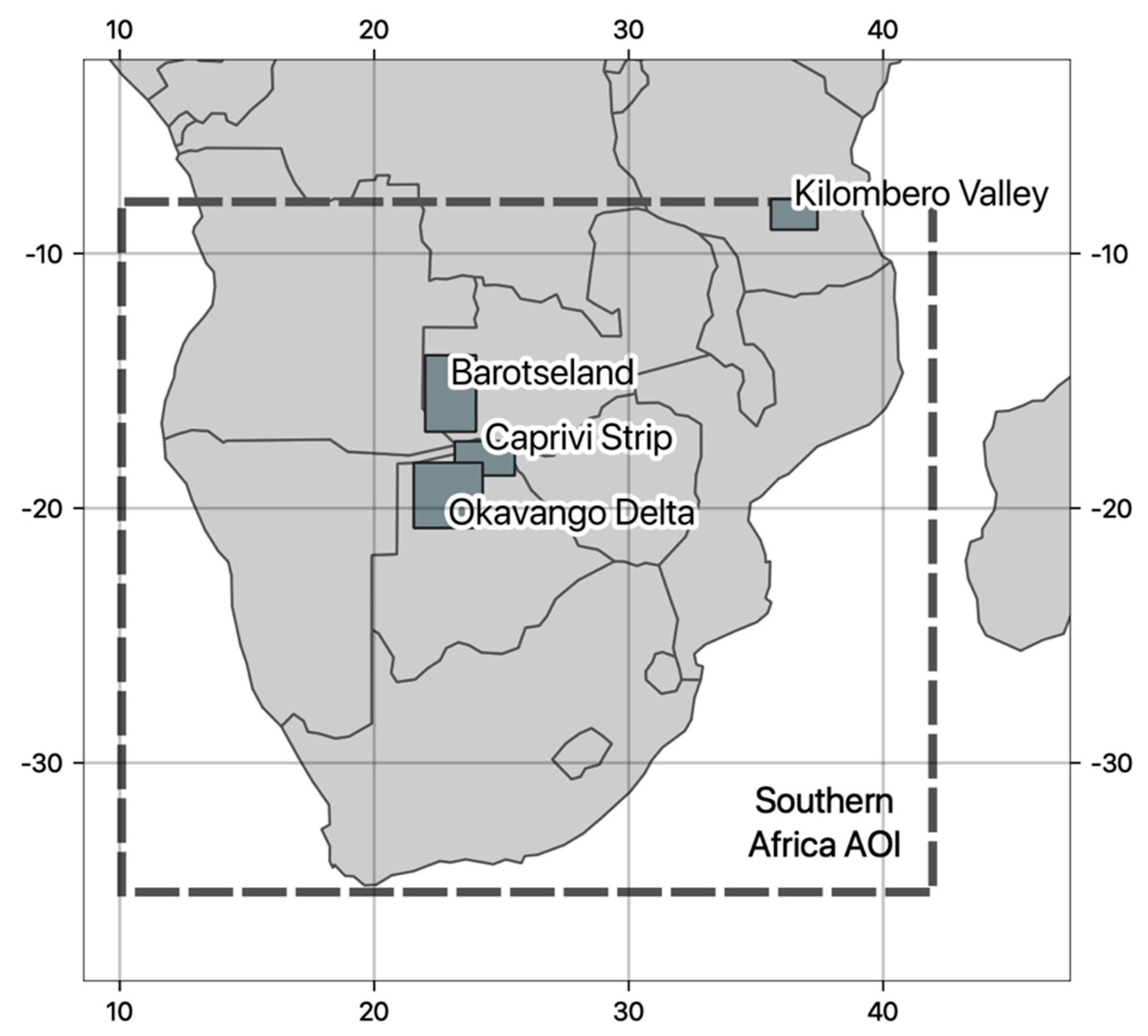
2.1. Study Areas

Four sites were selected for validating TropWet. These were: (1) Barotseland, Western Zambia, (2) the Zambezi Region, Namibia, (3) Okavango Delta, Botswana and (4) the Kilombero Valley, Tanzania (Figure 1). These sites are examples of large, seasonally inundated herbaceous-dominated wetlands in sub-Saharan Africa exhibiting high spatiotemporal variation in flood extent at the season scale. However, these are geographically disparate regions that feature differences in inundation dynamics, subsequent land cover distribution, and geology, thereby providing a rigorous test for the global applicability of the proposed technique. Alongside the four validation sites, TropWet was also applied to the Southern African nations (Angola, Namibia, South Africa, Botswana, Zimbabwe, Zambia, Swaziland, Lesotho, Malawi, and Mozambique) to demonstrate its use at broad spatial scales. These regions are briefly described below.

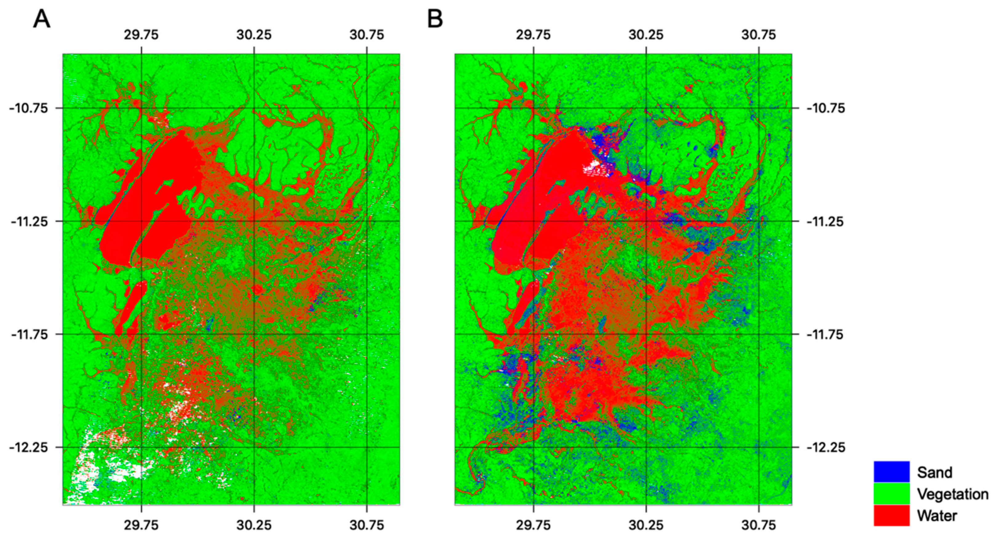
2.1.1. Barotseland, Western Zambia

The local geology in Barotseland is sedimentary, overlain by Kalahari sand, and localised silty alluvium within the floodplain [46]. Resistant basalt at the lower reaches of the floodplain causes the narrowing of the valley and the progression of seasonal backwaters upstream during peak flow conditions [47]. Dambos (waterlogged depressions) are situated predominately on the eastern escarpment of the floodplain. These pluvially fed features drain into the floodplain and tend to remain partially inundated during the dry season [47]. Floodplain vegetation is predominantly grassland and represents an important area for livestock rearing [47]. The region has a number of public health challenges including human nutrition, diseases like malaria, and access to health facilitates during periods of flooding [8]. Although flooding is widespread, it is not widely considered to be a significant hazard, but adapting to variabilities in flood timing and magnitude represents a significant challenge for local populations [46].

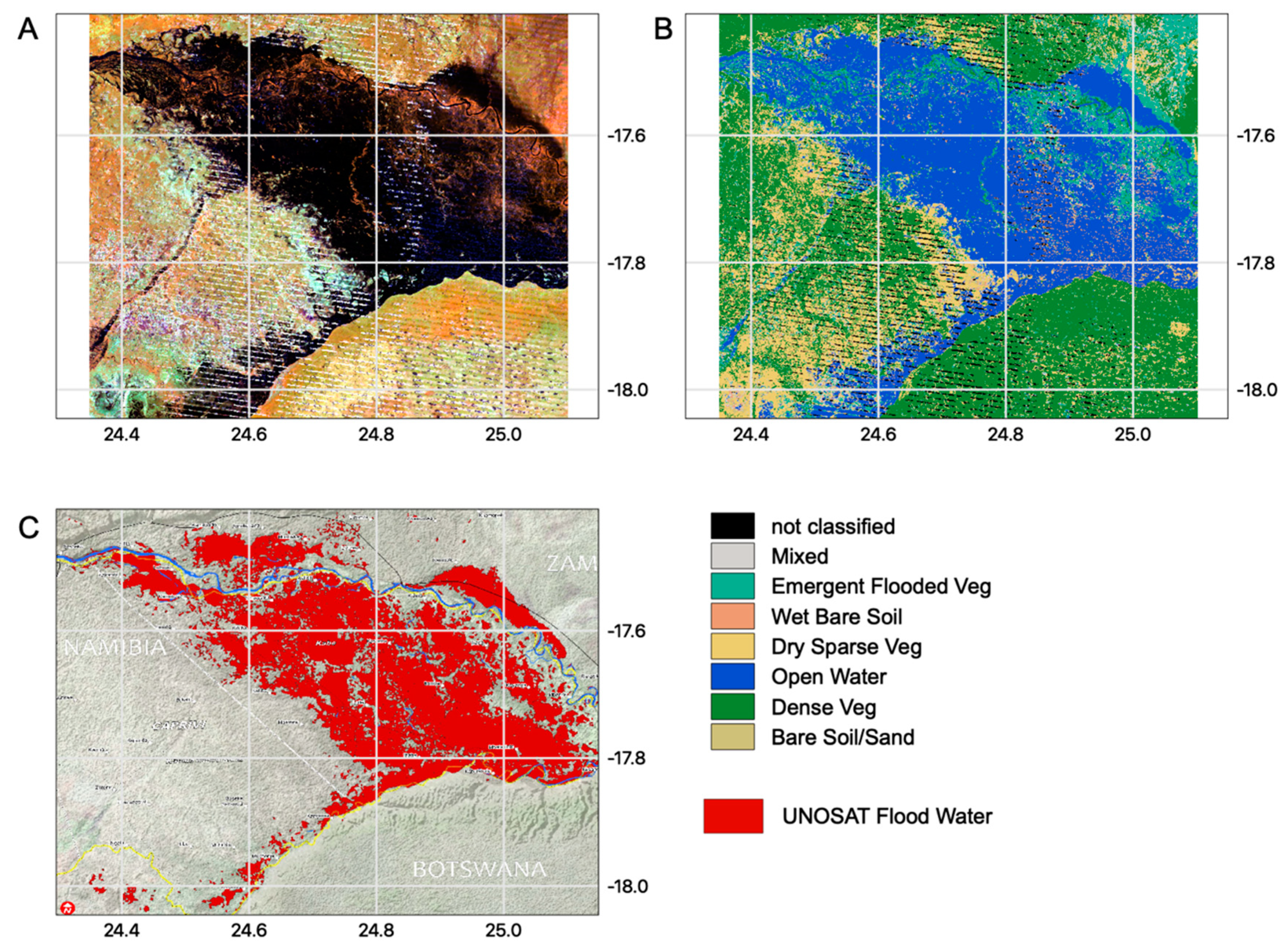
2.1.2. Zambezi Region, Namibia

The confluence of the Chobe River and Zambezi at the eastern edge of the Zambezi Region occurs over resistant basalt, resulting in backwater ponding during peak flow conditions [48,49]. The floodplain is dominated by a fine-grained sandy alluvium supporting tall grassland that is seasonally inundated. The area forms part of the Kavango–Zambezi Transfrontier Conservation Area (KAZA), a globally significant region for biodiversity including a key elephant migration route [49,50]. Flooding in this region is complex, being influenced by a number of different sources including a main flood pulse from the Zambezi River, backing up water into the Chobe system and a secondary flood pulse from the Kwando River via a combination of wetlands, lakes, and channels [50]. Apparent climate-change induced circulation pattern changes have resulted in extreme flood events (noticeably in 2009 and 2011) with devastating impacts for local communities [49,51,52]. The Zambezi Region is also a high-risk area for diseases like malaria [53], with transmission peaks timing with floodwater pulses [54].

2.1.3. Okavango Delta, Botswana

The Okavango Delta forms one of the world’s largest inland deltas [55,56]. Land cover is dominated by permanently inundated swampland and seasonally inundated grassland and forest [55,57]. Seasonal flooding is controlled by localised rainfall and floodwaters progressing downstream from the Angolan highlands between February and May [55], but this can take four months to propagate downstream due to the low topographic gradient of the region and restricted surface outflow channels, with peak flood extent occurring in the late dry season (August–October) [52,58]. The Delta has global significance in terms of wetland biodiversity and is recognised as a UNESCO (United Nations Educational, Scientific and Cultural Organization) World Heritage site [59,60]. Annual flooding in the Okavango wetlands provides a source of livelihood for ~125,000 people through the use of flood recession farming practices, therefore making local populations vulnerable to changes in the timing and magnitude of seasonal flooding [61,62]. The natural wetlands of the Okavango also provide extensive habitats for malarial mosquitoes, with the region accounting for the majority of malaria cases recorded across Botswana [63].

2.1.4. Kilombero Valley, United Republic of Tanzania

The Kilombero Valley is located within an asymmetrical half-graben between 30–40 km wide and 200 km long [64]. The area is a RAMSAR Convention recognised seasonal wetland with a largely distinct short (December–January) and long (March–May) rainy season [64,65]. The Kilombero Valley is one of the best characterised malaria transmission systems in Africa, having had some of the highest reported historical rates of malaria transmission [66]. Land use pressures related to population increases and overgrazing threaten the valley’s biodiversity including its Puku antelope population, which is estimated to make up three-quarters of the world’s population [67,68].

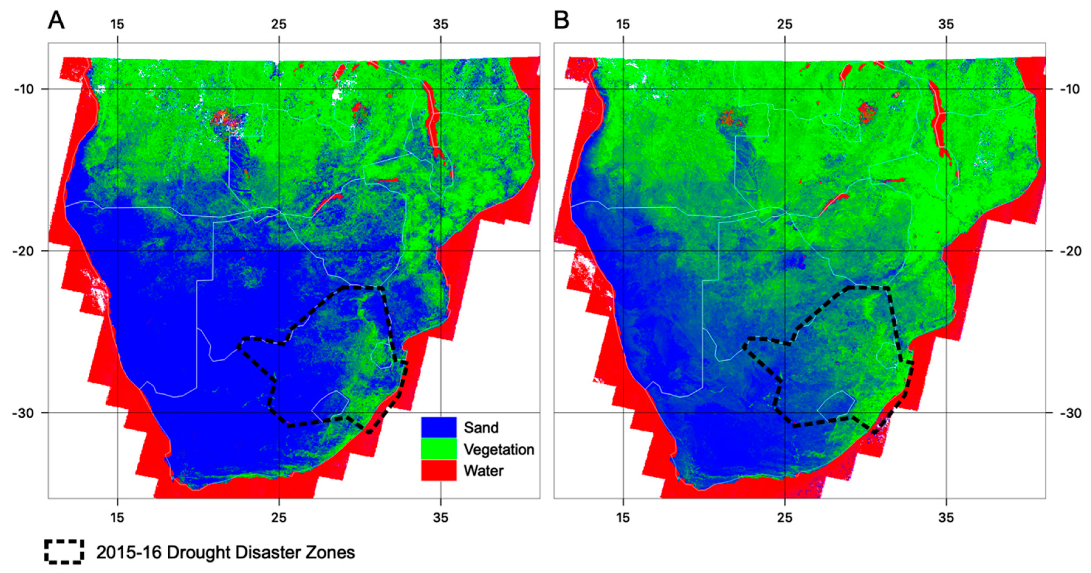
2.1.5. Southern African Countries

TropWet was also applied to the Southern Africa region including Angola, Namibia, South Africa, Botswana, Zimbabwe, Zambia, Swaziland, Lesotho, Malawi, and Mozambique (Figure 1). This region is vulnerable to the effects of global atmospheric circulation patterns such as the El Niño-Southern Oscillation (ENSO) and the Subtropical Indian Ocean Dipole (SIOD) [44,45]. Evidence shows that La Niña events coinciding with a positive SIOD can result in wetter than average conditions, whereas El Niño events coinciding with a negative SIOD phase can result in drier conditions [69]. To demonstrate the ability of the developed toolset for mapping the effects of these events, TropWet was applied to Southern Africa (Figure 1) for the months of December–March (the height of the wet season) in 2015–2016 and 2018–2019, representing significant drought and wetter than average conditions, respectively. This region was processed at a resolution of 1 km to ensure that the relevant processing did not exceed the maximum capacity of GEE.

2.2. Datasets

TropWet was developed for use with Landsat 5, 7, and 8 optical imagery, with a global revisit time of 16 days available since 1984. Spectral unmixing requires data to be processed to surface reflectance, eliminating the influence of atmospheric conditions. USGS Landsat 5, 7, and 8 Surface Reflectance Tier 1 imagery is ingested within the GEE system, following atmospheric correction made using the Landsat Ecosystem Disturbance Adaptive Processing System (LEDAPS: for Landsat 5 and 7) and the Landsat 8 Surface Reflectance Code (LaSRC) [70]. Prior to unmixing, each image underwent cloud and cloud shadow masking, using the pixel quality band associated with each Landsat image ingested into GEE, which was originally generated using the CFMask algorithm [71].

TropWet also uses information from terrain-based metrics to refine the classification process. We used the three arc-seconds (~90 m) SRTM Digital Surface Model product that is ingested into GEE (source: CGIAR: Consultative Group on International Agricultural Research).

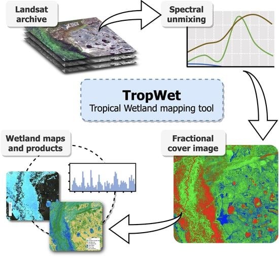
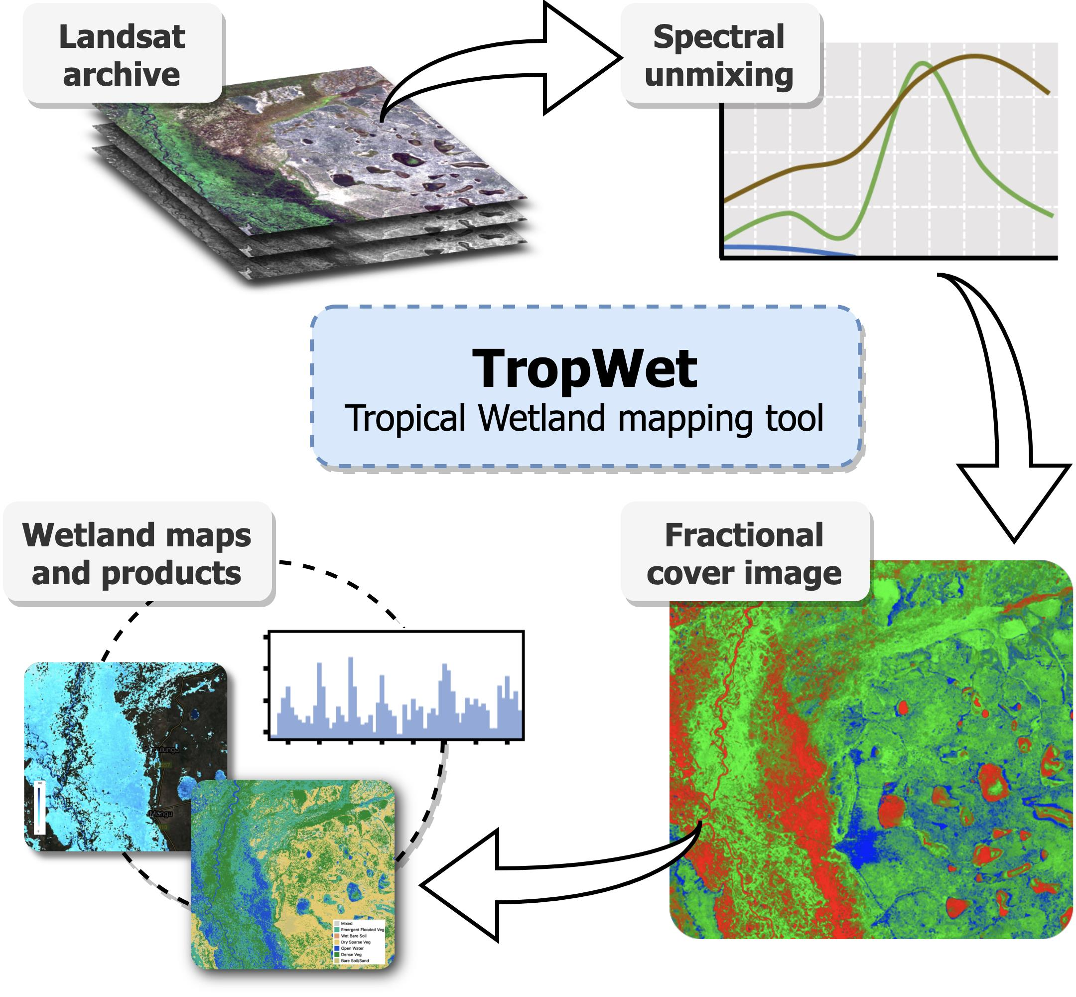
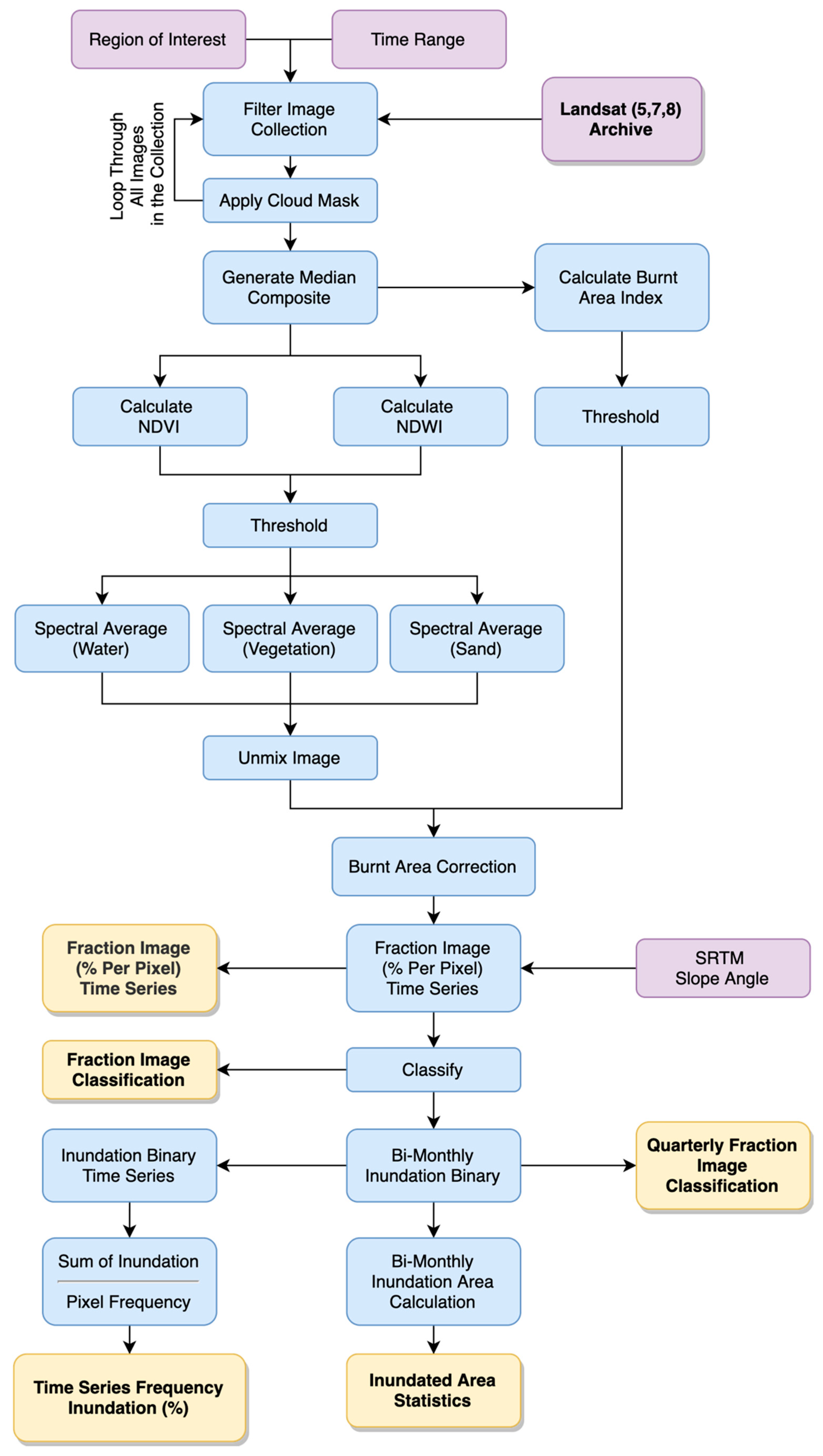
2.3. The TropWet Approach

An overview of the TropWet approach for mapping wetlands is given in Figure 2, outlining the unmixing approach applied to endmembers that are automatically extracted from input Landsat composites, generated over time periods and spatial extents that are defined by the user. The following sub-sections provide an explanation of these steps.

2.3.1. Linear Spectral Unmixing

The reflectance of a pixel can be conceptualised as a linear combination of the reflectance of all subpixel components (known as endmembers), weighted by abundance [41,72]. LSU uses this concept to calculate the fractional coverage of a pre-determined set of endmembers. LSU was performed in GEE, which uses spectral averaging to account for spectral variance for each endmember [73]. This is a computationally simple approach to unmixing and therefore lends itself to the analysis of large datasets compared to other more computationally expensive techniques like Multiple Endmember Spectral Mixture Analysis (MESMA) [74], which iteratively models every possible LSU combination of intra-endmember variation and endmember quantity on a pixel-by-pixel basis [75].

2.3.2. Automatic Endmember Selection

Pure spectra, or endmembers, for each class of interest are typically selected manually by an expert analyst, which can be a laborious and error prone process [76]. This study presents the novel concept of using the spectral indices NDVI (Normalised Difference Vegetation Index: Equation (1)) and mNDWI (modified Normalised Difference Wetness Index: Equation (2)) for the automatic selection of pure endmembers, allowing complete automation of the spectral unmixing procedure, vital for developing an operation monitoring system.

$$NDVI=\frac{\left(NIR-R\right)}{\left(NIR+R\right)}$$

(1)

$$mNDWI=\frac{\left(G-SWIR1\right)}{\left(G+SWIR1\right)}$$

(2)

The mixture model used in TropWet is based on three endmembers: (1) water, (2) photosynthetic (green) vegetation, and (3) sand (or bare soil/urban). This small set of endmembers enables the model to be over-determined (more wavebands than endmembers), an important requirement for the least square solution [77]. Additionally, by defining a relatively small number of broad classes, we can ensure applicability to wetland regions across the world, for instance, the sand endmember is suitable for other spectrally similar land cover types such as bare earth, exposed rock, and urban areas. Endmembers were defined using simple thresholding of the NDVI and mNDWI metrics (summarised in

Table 1. NDVI/mNDWI thresholds used for automatic pure endmember selection.

Endmember	NDVI	mNDWI
Water	-	>0.5
Vegetation	>0.7	-
Sand	>0.16 < 0.17	>−0.28 < 0.26

). These were determined by manually examining (by the same operator) the range of NDVI and mNDWI values over 900 regions of interest that represent pure spectra for each of the three endmembers (water, vegetation, and sand, N = 300 for each). This manual interrogation was carried out within GEE alongside high-resolution PlanetScope (3 m) reference imagery imported into GEE, guided by observations made in three field campaigns (March 2017, May 2018, and September 2018) over the Barotseland region in Western Zambia (Figure 1).

2.3.3. Accounting for Burn Regions

Throughout the tropics, grazing pastures often undergo burning (typically during the transition period between dry and wet seasons) to promote the regrowth of pasture. Freshly burned regions tend to be relatively dark, leading to spectral confusion between freshly burned pasture and open water, which can lead to an overestimation of surface water extent. To correct this, a novel application of the burn area index (BAI: Equation (3)) [78] was used as a post unmixing refinement.

$$BAI=\frac{1}{{\left(0.1-Red\right)}^2+{\left(0.06-NIR\right)}^2}$$

(3)

In this instance, BAI is used in conjunction with the unmixing result to determine areas that were incorrectly identified as open water. Specifically, these false positive pixels will have (i) a relatively high BAI value, (ii) a high fraction of water, and (iii) a low fraction of vegetation. The specific implication of this within TropWet is described in Equation (4).

$$BAI>\left(BA{I}_{mean}+BA{I}_{std}\right) \mathrm{AND} NDWS>-0.5<0.5 \mathrm{AND} V<10$$

(4)

where

$$NDWS=\frac{\left(W-S\right)}{\left(W+S\right)}$$

(5)

where NDWS is the normalised difference ratio between % fraction of water (W) and sand (S) and V is the % fraction of vegetation. For each burned pixel identified, the fraction of water is assumed to be sand/bare earth.

2.3.4. Terrain Based Masks

Terrain has a strong control on the hydrology of most landscapes. TropWet exploits this by using simple thresholds on standard terrain-based derivatives. The three arc-seconds (~90 m) SRTM Digital Surface Model is ingested into GEE. This was used to calculate slope angle and a threshold of 2.5° was used to restrict the prediction of wetlands to relatively flat slopes. Preference was given for the coarser three arc-seconds SRTM product (rather than the one arc-second version) as this suppresses small scale variations that might not be indicative of local hydrological conditions.

2.3.5. Surface Water Mapping Toolset and Exports

The surface water mapping toolset encompasses a total of four scripts. Each script is designed to generate a particular surface water product, as shown in

Table 2. Outputs from the surface water mapping toolset.

ID	Exportable Output
Thematic Classification	(i) Fraction image (%) (ii)Classified image (mixed; emergent flooded vegetation; wet bare sand; dry sparse vegetation; open water; dense vegetation; dry bare sand) (iii) Median composite image
Water Frequency	(i) Frequency of inundation (%) (ii) Mean fraction composite
Water Fraction Annual Statistics	(i) Chart and data with bi-monthly totals of open water and inundated vegetation area (number of pixels), alongside % of no data pixels
Quarterly Thematic Classifications	(i) 3 Monthly Composite Fraction Images (%) (ii) 3 Monthly Classified Images (mixed; emergent flooded vegetation; wet bare sand; dry sparse vegetation; open water; dense vegetation; dry bare sand)

, which can be exported and downloaded by the user. A brief description of each script is given below. The combined workflow for the surface water mapping toolset is shown in Figure 2.

The Tropical Wetland (TropWet) mapping tool is packaged into a single GEE toolbox containing four tools: (a) Thematic Classification, (b) Water Frequency, (c) Water Fraction Annual Statistics, and (d) Quarterly Thematic Classification.

The script can be accessed at the following link: https://www.aber.ac.uk/en/dges/research/earth-observation-laboratory/research/tropwet/.

(1)

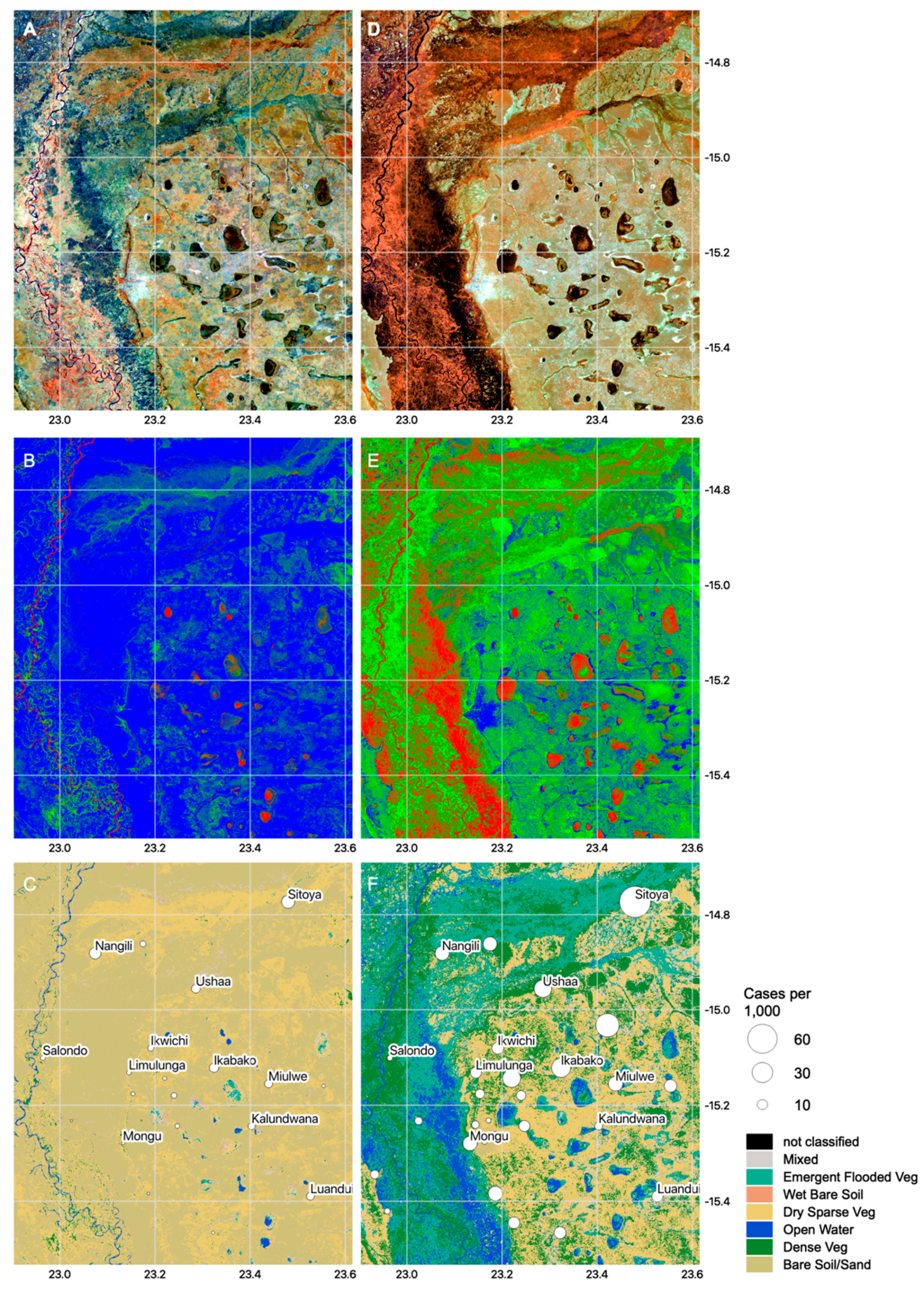
The Thematic Classification tool generates a median composite of cloud free Landsat 5, 7, or 8 for a designated date range and geographical area. Spectral endmembers are found and unmixing applied to determine the proportion (%) of water, vegetation, and sand for each pixel. This ‘fraction image’ is used to generate a thematic classification: (a) mixed, (b) emergent flooded vegetation, (c) wet bare sand, (d) dry sparse vegetation, (e) open water, (f) dense vegetation, and (g) dry bare sand, using rule-based thresholding.

(2)

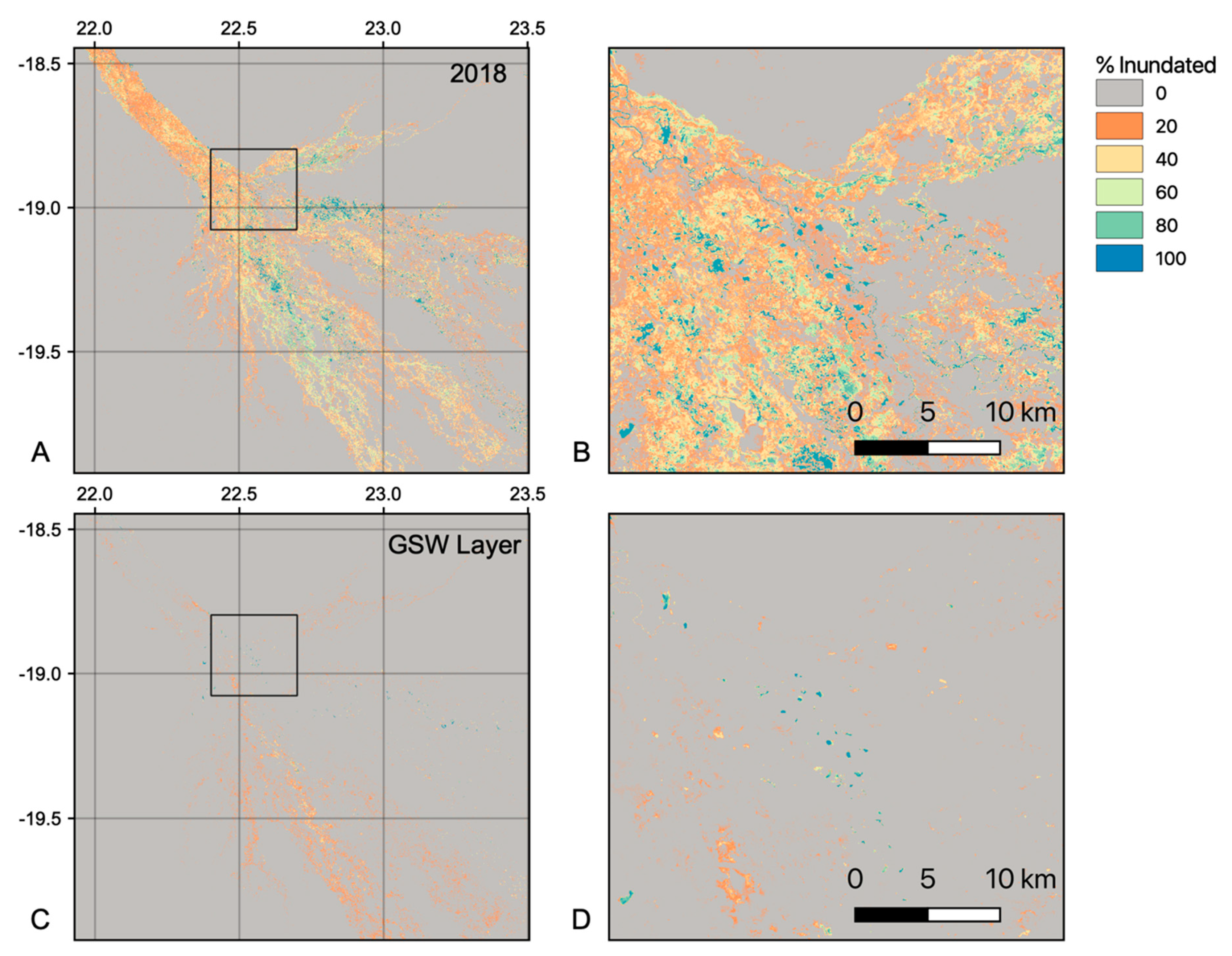
The Water Frequency tool generates a binary water extent layer, for every cloud free Landsat 5, 7, or 8 within a given date range. These binary layers are summed to produce a frequency of inundation, where the summed value represents the total number of times that water has been detected within the available images. This layer is expressed as a percentage.

(3)

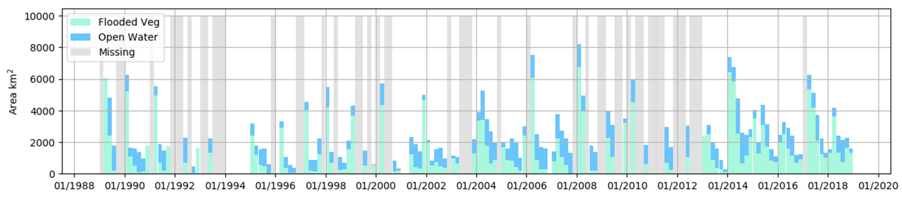
The Water Fraction Annual Statistics tool is used to generate annual statistics for a particular area of interest. Specifically, for each month within the given year, a median composite is generated from cloud free Landsat 5, 7, or 8, the endmembers are calculated, and unmixing applied. The resulting bi-monthly fractional coverage images are classified (using the rules described in

Table 3. Classification thresholds where: W = water; V = vegetation; S = sand; WV = water + vegetation; WS = water + sand; and VS = vegetation + sand.

Class	Class ID	Threshold (%)
Emergent Flooded Vegetation	EFV	WV ≥ 75 and V ≥ 25 < 75 and W ≥ 25 < 75
Wet Bare Sand	WBS	WS ≥ 75 and W ≥ 25 < 75 and S ≥ 25 < 75
Dry Sparse Vegetation	DSV	VS ≥ 75 and V ≥ 25 < 75 and S ≥ 25 < 75
Open Water	OW	W ≥ 75
Dense Vegetation	GV	V ≥ 75
Dry Bare Sand	DBS	S ≥ 75
Mixed/Other	M	-

to determine areas of inundated vegetation and open water. The total number of pixels for each class are then found and expressed as area coverage. This tool also outputs the number proportion of no data pixels, so that users can decide to ignore results where there are insufficient cloud free pixels available. The overall process is computationally intensive and is limited to run on a single year. Multiple years can be analysed by running the tool several times.

(4)

The Quarterly Thematic Classification tool is similar to the main classification tool but is designed to operate over a single year, and will return three monthly classified images for that year showing intra-annual change. The tool uses Landsat 5, 7, or 8 cloud free images for the periods: (a) January, February, and March; (b) April, May, and June; (c) July, August, and September; and (d) October, November, and December. These composite images are presented in GEE as clickable thumbnails that can added to the map for detailed analysis.

2.3.6. Thematic Classification

Single-date LSU uses a rule-based system based on fractional cover of water, vegetation and sand to classify the unmixed image into seven thematic classes (Table 3). If a pixel does not meet the set criteria of any of the six classes, it is considered to be a mixed region and is merged with cloud-masked regions to form the class mixed/other. Under this classification system, a pixel is allocated to a class where the fractional cover is greater than 75%. For example, pixels with a water fraction of ≥75% are classified as open water.

2.4. Accuracy Assessment

Accuracy assessment was conducted at four sites: Barotseland (Zambia), the Zambezi Region (Namibia), the Okavango Delta (Botswana), and the Kilombero Valley (Tanzania) (Figure 1). A total of 12 Landsat scenes were processed using TropWet, representing both the wet and dry seasons for each site, plus transitional periods where possible (

Table 4. Locations and dates of accuracy assessments made using 3 m PlanetScope imagery.

Region	Date	Season Description
Barotseland	07/08/2017	Dry season following recession of seasonal floodwaters
	08/09/2017	Dry season following recession of seasonal floodwaters
	24/09/2017	Dry season following recession of seasonal floodwaters
	14/01/2018	Rainy season prior to peak flow conditions within the floodplain
	20/04/2018	Peak flow conditions within the floodplain
	06/05/2018	Peak flow conditions within the floodplain
Kilombero Valley	16/09/2017	Dry season
	30/05/2018	Wet season
Zambezi Region	04/10/2017	Dry season
	15/05/2018	Wet season
Okavango Delta	07/08/2017	Dry season
	06/05/2018	Wet season

). Coincidental multi-spectral (blue, green, red, near-infrared) PlanetScope (3 m) imagery was used as reference imagery and accuracy points were visually interrogated alongside the TropWet classification result.

Overall, 10,800 points were generated for the accuracy assessment (

Table 5. Total number and distribution of accuracy assessment points.

Test Site	No. Points Per Class	No. Images	Site Total
Barotseland	100	6	3600
Kilombero Valley	200	2	2400
Zambezi Region	200	2	2400
Okavango Delta	200	2	2400
		Total	10,800

). Stratified random sampling was used to ensure that each class held an equal level of significance in the assessment of accuracy. Predicted and reference classes for each point were compared within a confusion matrix to derive overall accuracy. For the purpose of the confusion matrix, the six initial classes were merged and subset to four classes: (1) Sand (wet bare sand and dry bare sand); (2) Vegetation (dry sparse vegetation and dense vegetation); (3) Flooded Vegetation (emergent flooded vegetation) and; (4) Open Water (open water). This was done as it was not considered sufficiently possible to determine the difference between wet/dry soils or sparse/dense vegetation. It should be reaffirmed that emergent flooded vegetation as a class is confined to pixels with an open canopy structure as the intention of this toolset is to map water extent in herbaceous dominated wetlands.

Standard accuracy assessment metrics were calculated including the user’s and producer’s % agreement scores for each class and corresponding overall accuracy (%) and Kappa scores. Due to limitations in the Kappa score [79], we also calculated the quantity and allocation disagreement that describes how well the mapped products represent the area covered by each class (quantity disagreement) as well as the spatial agreement between mapped areas versus the validation data (allocation disagreement). A full description and discussion of these metrics can be found in Pontius and Millones [79].

3. Results

3.1. Classification Accuracy

Thematic classifications of water, bare sand, flooded emergent vegetation, and vegetation using the unmixing approach were shown to be highly accurate (

Table 6. Summary of accuracy assessment: Overall accuracy % (OA); kappa coefficient; Q: Quantity disagreement; A: Allocation disagreement; C: Overall agreement; D: Overall disagreement.

Date	ROI (sub-region)	OA (%)	kappa	Q	A	C	D
07/08/2017	Barotse (1)	90.2	0.87	0.20	0.01	0.79	0.21
	Barotse (2)	90.69	0.88	0.13	0.01	0.87	0.13
08/09/2017	Barotse (1)	90.69	0.88	0.12	0.03	0.87	0.13
	Barotse (2)	93.14	0.91	0.03	0.02	0.96	0.04
24/09/2017	Barotse (1)	90.69	0.88	0.12	0.03	0.86	0.14
	Barotse (2)	89.22	0.86	0.22	0.03	0.76	0.24
14/01/2018	Barotse (1)	90.2	0.87	0.13	0.01	0.86	0.14
	Barotse (2)	87.75	0.84	0.20	0.00	0.80	0.20
20/04/2018	Barotse (1)	95.1	0.93	0.07	0.00	0.92	0.08
	Barotse (2)	90.1	0.87	0.10	0.02	0.88	0.12
06/05/2018	Barotse (1)	87.25	0.83	0.10	0.04	0.86	0.14
	Barotse (2)	88.94	0.85	0.07	0.04	0.89	0.11
16/09/2017	Kilombero	95.43	0.94	0.08	0.00	0.91	0.09
30/05/2018	Kilombero	91.67	0.9	0.09	0.00	0.91	0.09
04/10/2017	Caprivi	90.1	0.87	0.00	0.02	0.99	0.01
15/05/2018	Caprivi	95.92	0.95	0.01	0.00	0.98	0.02
07/08/2017	Okavango	92.48	0.91	0.04	0.01	0.96	0.04
06/05/2018	Okavango	88.12	0.85	0.10	0.01	0.89	0.11
Mean		91.0	0.88	0.10	0.02	0.89	0.11
Std. dev.		2.6	0.03	0.06	0.01	0.06	0.06

: mean overall accuracy 91%, st. dev. 2.6%, n = 10,800) across the four validation sites at different times of the hydrological year. This consistency shows that TropWet can provide accurate assessments of wetland coverage for a range of herbaceous regions across sub-Saharan Africa. Given that these classifications were generated using endmembers extracted automatically from the area of interest (based on thresholding commonly used band indices: NDVI, mNDWI), we are confident that the developed approach can be transferred to other regions across the world with no user input. The classification approach itself was calibrated on the Barotseland region, however, there was no reported difference in accuracy scores between this site and the other validation sites, again, demonstrating transferability of the approach to other tropical wetlands.

The combined error matrix (

Table 7. Combined error matrix (% of N = 10,800) where: W = water; S = sand; FV = emergent flooded vegetation; V = vegetation.

	W	S	FV	V	User (%)
W	27.22	0.65	1.32	0.00	93.29
S	1.06	27.23	0.05	0.65	94.09
FV	2.00	0.20	26.67	0.32	90.85
V	0.13	1.53	1.34	31.67	93.07
Producer (%)	88.05	94.53	90.37	97.85	92.41
OA (%)	92.41
kappa	0.89

: N = 10,800) demonstrates high agreement across all classes, with error predominantly confined to the confusion of flooded vegetation with water, and water with sand. The incorrect identification of sand areas as open water was primarily due to the presence of residual regions of burnt areas that were not corrected by the burn mask. Additionally, some areas with saturated dark soils were incorrectly classified as open water due to their spectral similarity.

3.1.1. Barotseland

TropWet was applied to a 6210 km² area in Barotseland Western Zambia for the dry season (March–May) and wet season (September–November) of 2017 at a target resolution of 30 m. The fractional cover and corresponding thematic classification maps (Figure 3) demonstrate that the area is hydrological very dynamic: dry season surface water availability is largely restricted to the main Zambezi channel and circular raised peat bogs on the escarpment, whereas the wet season is characterised by widespread inundation with almost the entire floodplain being covered in either open water or inundated vegetation, although it is likely that the areas of dense vegetation close to the channel are areas of dense matted grasses or floating vegetation that cannot be detected by TropWet.

The region has a number of important public health challenges including malaria burden. African malarial mosquitoes tend to rely on shallow, stagnant, or slow-moving water bodies for oviposition and larval development [80]. The circular dambo hydrological features are characteristic of such habitats and are shown by TropWet to be inundated in both the wet and dry season, resulting in relatively high malaria case rates at Ikabako, Luandui, and Miulwe. High rates at Situoya to the northeast of the area are also coincidental with slow-moving shallow water bodies associated with a braided tributary system [8]. By using TropWet to characterise wetlands in malaria endemic regions can help to target interventions such as the treating of malarial mosquito aquatic habitats with larvicide.

3.1.2. Okavango Delta

TropWet was applied to a 21,030 km² area of the Okavango Delta from 1989 to 2018 at a target resolution of 30 m. Inundation extents were only reported where a cloud free composite (cloud cover <10%) could be generated for a two-month block. For the Okavanko Delta, 29% of the two-month blocks over the period 1989–2018 had available cloud free composites (Figure 4). The extent of inundation was shown to be highly variable with a mean inundated area of 2479 km², but a standard deviation of 1727 km², and a maximum extent of 8210 km² (Feb 2008), representing over 39% of the total studied area as being inundated with water. The annual distribution of mapped open water showed a tendency for the flood peak to occur in May–August, with a high degree of fluctuation in the timing and extent of the flood peak (

Table 8. Distribution of open water inundation (km²) for the Okavango Delta from 1989–2018.

Two-Month Block	n	Mean	Min	Max	St. Dev.
Jan–Feb	17	543	1	1477	440
Mar–Apr	24	810	2	1865	497
May–Jun	22	1354	663	2383	485
Jul–Aug	22	1380	510	2280	412
Sep–Oct	23	827	5	1480	387
Nov–Dec	16	296	6	923	245

).

The fluctuation in flood timing and magnitude has implications for a range of application areas. Seasonally flooded zones during peak flood periods can represent a significant increase (>300%) in dissolved inorganic carbon concentrations compared to permanently wetted areas at the head of the Delta [81]. Using tools like TropWet may therefore contribute to efforts to quantify greenhouse gas flux in major wetland areas, which represents a key uncertainty in current regional and global climate change models. The fluctuation vegetation and inundated vegetation, particularly during the flood drawdown period, at the onset of the dry season, represents an important metric for quantifying forage materials that are key for wildlife dynamics in the area such as elephant migration [60]. Using TropWet can therefore provide proxy indicators of habitat suitability and the change in suitability over time. Additionally, the livelihoods for ~125,000 people are reliant on the annual pulse of floodwater in the Okavango Delta, particularly through the use of flood recession farming practices [61,62]. Uncertainty in the timing and magnitude of the annual flood waters can make local populations vulnerable, particularly in times of drought [62]. By using TropWet, the variation in flood water extent, onset, and duration can be used to determine effects on livelihoods and help to mitigate against future drought events.

Previous attempts to map this region have shown the extent of inundation to be between 4000 and 13,000 km² [56], more extensive than the estimates made by TropWet. On one hand, this may be due to the degree of water underneath dense vegetation canopies that would not be identified by the unmixing process. However, equally, the difference may be due to relatively fine granularity of the TropWet Landsat-based product (30 m) compared to the previous estimates that were based on 1 km AVHRR (Advanced Very-High-Resolution Radiometer) pixels that will not capture finer scale features such as islands within the extensive braided river system, possibly leading to an overestimation of flood water extent. Future work may consider a direct comparison between coarser scale extent maps, TropWet-derived extent maps, and field observation to determine the true extent of inundated area in the Okavango Delta.

The granularity of the TropWet-derived product is illustrated in Figure 5A,B that shows a % frequency inundation map for 2018. Here, permanently inundated channels and pools are mapped alongside transitional zones and permanently dry islands within the braided deltaic region and the permanently dry escarpment lying outside the Delta region. Conversely, Figure 5C,D show the equivalent inundation frequency product from the Global Surface Water Explorer (GSW) [33], a globally available product, also generated using Landsat imagery within the GEE platform. The contrast between the two products demonstrates the value of the unmixing approach, enabling users to quantify inundation in partially vegetated pixels, whereas the GSW product can only identify open water pixels. The advantages of TropWet are particularly apparent in this example because the GSW map was created using the entire Landsat archive, whereas the TropWet was only generated using 2018 data.

3.1.3. Zambezi Region, Namibia

The Zambezi Region represents a significant habitat for a number of species including the critically endangered wild dog as well as acting as a vital migration corridor for a range of herbivore species such as elephant [49]. Much of this biodiversity is reliant on the annual pulse of floodwater, originating from the Angolan Highlands. The area is also highly populated and local populations are vulnerable to the effects of flooding including widespread displacement of people and cattle. Knowledge of the extent floodwater inundation can be vital for directing relief efforts, public health management as well as planning mitigation strategies [2]. In 2009, the region experienced widespread flooding leading to the displacement of 56,000 people [82]. As one of the largest flood events recorded in the region over last four decades [50], we decided to use this event to demonstrate the potential for TropWet to provide information on historic flood events as an example of a case study

TropWet was applied to the Zambezi Region for March 2009 at a target resolution of 30 m. The fractional cover product as well as the thematic classified image is shown in Figure 6 alongside an ENVISAT-ASAR (Environmental Satellite – Advanced Synthetic Aperture Radar) radar-derived delineation of flood water extent generated by the United Nations Institute for Training and Research Operational Satellite applications programme (UNITAR-UNOSAT), who provide rapid response maps of flooding event for humanitarian relief. The TropWet-derived map showed strong agreement with the UNOSAT product, although TropWet was able to detect a greater extent of inundation by also considering inundated vegetation as well as open water, demonstrating the effectiveness of TropWet. However, missing data due to cloud cover and the Landsat 7 scan-line error suggests that although retrospective assessments of floodwater extent are possible with TropWet, approaches designed for near real-time rapid response mapping should utilise radar imagery that is not affected by cloud cover.

3.1.4. Southern Africa

The combination of the El Niño-Southern Oscillation and the SIOP is known to affect precipitation patterns across Southern Africa [44,45,84]. TropWet was applied to this region for two periods: (1) La Niña and positive SIOD phase (December 2018 to March 2019) producing wetter than average conditions and (2) El Niño and negative SIOD phase (December 2015 to March 2016) representing drier than average conditions. TropWet, applied with a target resolution of 1 km, was able to deliver widescale assessments of the impact of fluctuations in atmospheric circulation patterns. In this instance, the Southern African region experienced a greatly reduced extent of green vegetation between these two events (Figure 7), equivalent to 183.2 million ha in 2015–2016 and 261.6 million ha in 2018–2019. This is representative of a vast reduction in crops or grasses for domestic herbivores during El Niño events with serious consequences for food and social security [44,85,86,87].

The regions of KwaZulu-Natal, North West, Free State, Limpopo, and the Northern Cape were declared to be drought disaster zones during the 2015–2016. For this region, TropWet demonstrated an 80% difference in green vegetation between the wet seasons of 2015–2016 and 2018–2019 (Figure 7), equivalent to a difference of 7.25 million ha. The direct implications of this was drastically reduced maize yields in 2015–2016 compared to previous years, leading to a widespread impact on the health and wellbeing of people in this region [85,86]. The Southern African region also includes a number of globally significant wetland habitats that demonstrated a significant difference in wet season surface water extent between 2015–2016 and 2018–2019. Specifically, the Bangweulu Swamps, cited by the RAMSAR convention as one of the world’s most important wetland habitats, had a 30% difference in surface water extent between 2015–2016 and 2018–2019, equivalent to 169 thousand ha (Figure 8). This variation has important consequences for a range of threatened and endangered species (e.g., black lechwe, wattle crane, shoebill stork) as well as implications for fisheries, with the Bangweulu Swamps representing the largest fishery in Zambia due to its species diversity and importance for breeding and spawning [88,89].

4. Discussion

With overall accuracy scores exceeding 91%, we have shown that a simple mixture model can provide accurate maps of wetland extent for the monitoring and assessment of tropical wetlands using freely available Landsat imagery. By considering the sub-pixel level fractional cover of water and vegetation, users are able to map the extent of both open water and inundated vegetation. As a result, TropWet is able to identify a much greater extent in inundation for regions like the Okavango Delta compared to other globally available systems such as the Global Surface Water Explorer, which was designed to identify and map open water.

TropWet uses fractional cover of water, vegetation, and bare sand to derive a thematic classification of inundation extent. Although the system was calibrated for Barotseland, Western Zambia, there was remarkably little difference in accuracies for other sites in sub-Saharan Africa, demonstrating the robustness of the automated approach and its subsequent transferability. This represents an exciting potential for making continental-scale assessments of inundation frequency and extent, nevertheless, thresholds used to generate the thematic map can be adapted by the user and adapted for specific regions if needed. Indeed, the nomenclature for the thematic map was designed for ecohydrological characterisation, but this can be adapted for other class types to target other applications such as mapping terrestrial vegetation loss, vegetation fragmentation [90], and desertification (e.g., [91,92,93]).

TropWet was developed for herbaceous wetland regions, mainly due to the inability of optical satellite imagery such as Landsat to provide information about water bodies underneath dense vegetation canopies such as forests. One possible solution is to include information from the Normalised Difference Infrared Index (NDII), which has been shown to provide reliable classifications of aquatic vegetation [94]. An alternative solution is to integrate radar imagery for mapping land cover underneath vegetation canopies and is particularly valuable for flood mapping, given its independence of cloud cover conditions. L-band radar imaging systems would provide the best potential for making these assessments [35,36,95]. Although it is encouraging to report accuracies associated with mapping inundated vegetation using TropWet equivalent to those reported by approaches that use L-band imagery [32,35] or GNSS-R [21,23,24], it should be reiterated that TropWet is limited to inundated grassland environments. However, L-band imagery archives are not currently ingested within GEE. More importantly, archives of radar imagery do not match the temporal extent and frequency of the Landsat archive, meaning that long-term assessments of wetland extent and inundation frequency are challenging. Integration with optical Sentinel-2 imagery, with its superior spatial resolution and revisit time, would provide additional data for TropWet to make assessments of inundation in a more timely and precise manner. However, the absence of a thermal band makes cloud masking problematic at present [96].

TropWet is implemented in the open source GEE platform. This enables widespread availability, meaning that non-expert users can use the system and apply it to their own areas of interest. This also gives users to ability to process decades worth of data over relatively large areas, a task that would require a great deal of computational resources if carried out using locally-based systems. In the example of the Okavango Delta, the 1.8 million ha area would require downloading and processing four Landsat tiles (path 174–175, row 73–74) representing between 2 GB (Landsat 5) and 6.44 GB (Landsat 8) for a single epoch. The analysis carried out in this paper considered all available scenes between 1988–2018 with 23 potential epochs per year (16-day revisit period), which represents a significant amount of data (max potential 92 scenes per year x 30 years = 2760 scenes in total, although gaps exist in the archive) that would exceed the resource capabilities for many organisations. TropWet allows for the analysis of wetlands to take place at a temporal and spatial scale that is suitable for informing national and regional scale policies.

With the ability to process and analyse over 30 years’ worth of Landsat data, TropWet can be used to establish seasonal patterns in inundation extent. By mapping the variation in inundation extent, we can help to quantify the contribution of large tropical wetlands to greenhouse gas flux, a potentially important uncertainty for regional and global climate change modelling [15]. By mapping seasonal inundation patterns TropWet also provides a vital tool for the targeting of public health resources to tackle water-borne disease. For instance, characterising inundation frequency in malaria endemic regions—as has been demonstrated for Barotseland, Western Zambia—provides targets for interventions such as larval source management: treating water bodies where malarial mosquitoes breed using larvicide (e.g., [97,98]).

The performance of TropWet for mapping open water (user’s accuracy: 93%, producer’s accuracy: 88%) is equivalent to accuracies reported by approaches based on radar imagery [1,2,3,4,5,6,7]. As discussed previously, radar is better suited to an operational flood hazard mapping system (mainly due to its independence from cloud conditions), but our encouraging results demonstrate that TropWet can be used to make retrospective assessments of historic flood extent. In doing so, TropWet can be used to plan mitigation strategies for returning events. This is particularly valuable for large scale, resource poor regions (lack of hydrometric data and precise digital terrain data necessary for hydraulic modelling) where reliable flood modelling and subsequent flood-risk mapping is not possible. Furthermore, the density of data over the Landsat archive also enables users to make assessment of long-term events, for instance, establishing peak flood water extents during El Niño or La Niña events. In this respect, these recurring patterns could be used to mitigate the effects of these events by establishing the typical availability of surface water during previous events, whether that be water scarcity or excess of water leading to flood hazard. This also means that TropWet has the ability to assess the impact of atmospheric circulation pattern changes over large spatial scales. In this paper, we demonstrated the ability of TropWet to identify significant changes in the extent of green vegetation over the Southern African region. In this manner, TropWet is able to support on-going efforts to quantify the specific effects of variations in El Niño or La Niña events (e.g., [44]). In doing so, policy makers have a tool to examine the implications of these events and help mitigate against them.

Limitations

TropWet aims to map open water and inundated vegetation within herbaceous dominated wetland systems and is not applicable to areas with dense canopy covers (i.e., forests). Additionally, fieldwork within the Bartoseland region and the Kilombero Valley revealed that extensive floating vegetation or matted grasses can similarly mask water underneath that, again, would not be detected by the optical-unmixing approach. The TropWet derived inundation maps and subsequent accuracy assessment are, therefore, representative of inundated pixels where at least 25% of the pixel is not covered by dense vegetation.

Cloud cover remains the major limiting factor for all optically-based EO monitoring systems. Users of TropWet need to bear this in mind when analysing their areas of interest. In some instances, regions are relatively cloud free, particularly in particular seasons, in which case, relatively dense time-series can be explored. However, in regions where cloud cover is persistent, users may find it beneficial to examine broader temporal scale patterns in inundation. For instance, rather than trying to obtain yearly maps of wet season inundation frequency for an area, the user may consider deriving inundation frequency within wet season months over a 10-year period, thereby maximising the chance of obtaining a suitable number of cloud free pixels. Additionally, the Landsat archive is not continuous. For instance, during the period 1984 to 1999, the Landsat programme was commercialised, meaning that scenes were only acquired where there was a buyer leaving a gap in the archive for a number of regions, particularly Sub-Saharan Africa.

Although TropWet harnesses the archives of analysis ready data and processing capabilities of GEE, there are restrictions on the computing resources accessible to a single user. GEE hardware uses a parallelised cluster computer infrastructure that physically limits the amount of data that can be stored and consequently processed on a single cluster node [37]. In addition, the cloud based nature of the infrastructure imposes reasonable user limits to allow fair usage for all (April 2020): (a) A computational time limit of 270 seconds is applied for individual processing operations, (b) 40 simultaneous low intensity operations (band math and general per pixel analysis), and (c) 25 simultaneous high intensity operations (spatial aggregation on a per image basis) [37]. For intensive operations, a maximum number of pixels that can be processed is set at 1 billion pixels and is somewhat independent to the area that can be processed, as pixel resolution can be adjusted to increase the processable area. Maintaining the native 30 m resolution of Landsat 5, 7, and 8, it would theoretically be possible to apply the model to an area of approximately 900,000 km².

5. Conclusions

We presented a new tool for providing accurate maps of wetland extent including discrimination of both open water bodies and flooded vegetation by considering the sub-pixel fractional cover of water, vegetation, and sand/bare soil. TropWet employs a simple unmixing approach applied to optical Landsat imagery. Although simplistic, this automated approach was shown to be transferable across a number of representative sites across Africa.

By using imagery from the long-term Landsat mission, TropWet users are able to make historical assessments of wetland extent and dynamics. By exploiting the cloud-based GEE processing resources, TropWet can be used to conduct large scale analyses over broad timescales, making it suitable for informing national and international level land management decisions. Furthermore, by implementing TropWet in GEE, it is made available to a broad spectrum of users including both experts and non-experts, independent of computational resource availability. In this study, we demonstrated the potential for TropWet to provide geographical information to help tackle key environmental and public health challenges including malaria control, flood hazard mitigation, conservation, and quantifying the effects of changes in global climate circulation patterns.

References

- Twele, A.; Cao, W.; Plank, S.; Martinis, S.; Cao, W.; Plank, S. Sentinel-1-based flood mapping: A fully automated processing chain. Int. J. Remote Sens. 2016, 37, 2990–3004. [Google Scholar] [CrossRef]
- Bioresita, F.; Puissant, A.; Stumpf, A.; Malet, J.-P. A Method for Automatic and Rapid Mapping of Water Surfaces from Sentinel-1 Imagery. Remote Sens. 2018, 10, 217. [Google Scholar] [CrossRef] [Green Version]
- Westerhoff, R.S.; Kleuskens, M.P.H.; Winsemius, H.C.; Huizinga, H.J.; Brakenridge, G.R.; Bishop, C. Automated global water mapping based on wide-swath orbital synthetic-aperture radar. Hydrol. Earth Syst. Sci. 2013, 17, 651–663. [Google Scholar] [CrossRef] [Green Version]
- Martinis, S.; Kersten, J.; Twele, A. A fully automated TerraSAR-X based flood service. ISPRS J. Photogramm. Remote Sens. 2015, 104, 203–212. [Google Scholar] [CrossRef]
- Pulvirenti, L.; Pierdicca, N.; Chini, M.; Guerriero, L. An algorithm for operational flood mapping from Synthetic Aperture Radar (SAR) data using fuzzy logic. Nat. Hazards Earth Syst. Sci. 2011, 11, 529–540. [Google Scholar] [CrossRef] [Green Version]
- DeVries, B.; Huang, C.; Armston, J.; Huang, W.; Jones, J.W.; Lang, M.W. Rapid and robust monitoring of flood events using Sentinel-1 and Landsat data on the Google Earth Engine. Remote Sens. Environ. 2020, 240, 111664. [Google Scholar] [CrossRef]
- Huang, W.; DeVries, B.; Huang, C.; Lang, M.; Jones, J.; Creed, I.; Carroll, M. Automated Extraction of Surface Water Extent from Sentinel-1 Data. Remote Sens. 2018, 10, 797. [Google Scholar] [CrossRef] [Green Version]
- Hardy, A.; Ettritch, G.; Cross, D.E.; Bunting, P.; Thomas, C.C.; Liywalii, F.; Sakala, J.; Silumesii, A.; Singini, D.; Smith, M.; et al. Automatic detection of open and vegetated water bodies using Sentinel 1 to map African malaria vector mosquito breeding habitats. Remote Sens. 2019, 11, 593. [Google Scholar] [CrossRef] [Green Version]
- Bøgh, C.; Lindsay, S.W.S.; Clarke, S.E.S.; Dean, A.; Jawara, M.; Pinder, M.; Thomas, C.J. High spatial resolution mapping of malaria transmission risk in the Gambia, West Africa, using Landsat TM satellite imagery. Am. J. Trop. Med. Hyg. 2007, 76, 875–881. [Google Scholar] [CrossRef]
- Behnamian, A.; Banks, S.; White, L.; Brisco, B.; Millard, K.; Pasher, J.; Chen, Z.; Duffe, J.; Bourgeau-Chavez, L.; Battaglia, M. Semi-Automated Surface Water Detection with Synthetic Aperture Radar Data: A Wetland Case Study. Remote Sens. 2017, 9, 1209. [Google Scholar] [CrossRef] [Green Version]
- Schlaffer, S.; Chini, M.; Dettmering, D.; Wagner, W. Mapping Wetlands in Zambia Using Seasonal Backscatter Signatures Derived from ENVISAT ASAR Time Series. Remote Sens. 2016, 8, 402. [Google Scholar] [CrossRef] [Green Version]
- Clewley, D.; Whitcomb, J.; Moghaddam, M.; McDonald, K.; Chapman, B.; Bunting, P. Evaluation of ALOS PALSAR data for high-resolution mapping of vegetated wetlands in Alaska. Remote Sens. 2015, 7, 7272–7297. [Google Scholar] [CrossRef] [Green Version]
- Brisco, B.; Li, K.; Tedford, B.; Charbonneau, F.; Yun, S.; Murnaghan, K. Compact polarimetry assessment for rice and wetland mapping. Int. J. Remote Sens. 2013, 34, 1949–1964. [Google Scholar] [CrossRef] [Green Version]
- Bwangoy, J.-R.B.; Hansen, M.C.; Roy, D.P.; De Grandi, G.; Justice, C.O. Wetland mapping in the Congo Basin using optical and radar remotely sensed data and derived topographical indices. Remote Sens. Environ. 2010, 114, 73–86. [Google Scholar] [CrossRef]
- Borges, A.V.; Darchambeau, F.; Teodoru, C.R.; Marwick, T.R.; Tamooh, F.; Geeraert, N.; Omengo, F.O.; Guérin, F.; Lambert, T.; Morana, C.; et al. Globally significant greenhouse-gas emissions from African inland waters. Nat. Geosci. 2015, 8, 637–642. [Google Scholar] [CrossRef] [Green Version]
- Dargie, G.C.; Lewis, S.L.; Lawson, I.T.; Mitchard, E.T.A.; Page, S.E.; Bocko, Y.E.; Ifo, S.A. Age, extent and carbon storage of the central Congo Basin peatland complex. Nature 2017, 542, 86–90. [Google Scholar] [CrossRef]
- Schroeder, R.; McDonald, K.; Chapman, B.; Jensen, K.; Podest, E.; Tessler, Z.; Bohn, T.; Zimmermann, R. Development and Evaluation of a Multi-Year Fractional Surface Water Data Set Derived from Active/Passive Microwave Remote Sensing Data. Remote Sens. 2015, 7, 16688–16732. [Google Scholar] [CrossRef] [Green Version]
- Poulter, B.; Bousquet, P.; Canadell, J.G.; Ciais, P.; Peregon, A.; Saunois, M.; Arora, V.K.; Beerling, D.J.; Brovkin, V.; Jones, C.D.; et al. Global wetland contribution to 2000–2012 atmospheric methane growth rate dynamics. Environ. Res. Lett. 2017, 12, 094013. [Google Scholar] [CrossRef]
- Papa, F.; Prigent, C.; Aires, F.; Jimenez, C.; Rossow, W.B.; Matthews, E. Interannual variability of surface water extent at the global scale, 1993–2004. J. Geophys. Res. 2010, 115, D12111. [Google Scholar] [CrossRef]
- Du, J.; Kimball, J.S.; Galantowicz, J.; Kim, S.-B.; Chan, S.K.; Reichle, R.; Jones, L.A.; Watts, J.D. Assessing global surface water inundation dynamics using combined satellite information from SMAP, AMSR2 and Landsat. Remote Sens. Environ. 2018, 213, 1–17. [Google Scholar] [CrossRef]
- Rodriguez-Alvarez, N.; Podest, E.; Jensen, K.; McDonald, K.C. Classifying Inundation in a Tropical Wetlands Complex with GNSS-R. Remote Sens. 2019, 11, 1053. [Google Scholar] [CrossRef] [Green Version]
- Morris, M.; Chew, C.; Reager, J.T.; Shah, R.; Zuffada, C. A novel approach to monitoring wetland dynamics using CYGNSS: Everglades case study. Remote Sens. Environ. 2019, 233, 111417. [Google Scholar] [CrossRef]
- Nghiem, S.V.; Zuffada, C.; Shah, R.; Chew, C.; Lowe, S.T.; Mannucci, A.J.; Cardellach, E.; Brakenridge, G.R.; Geller, G.; Rosenqvist, A. Wetland monitoring with Global Navigation Satellite System reflectometry. Earth Sp. Sci. 2017, 4, 16–39. [Google Scholar] [CrossRef] [PubMed]
- Jensen, K.; McDonald, K.; Podest, E.; Rodriguez-Alvarez, N.; Horna, V.; Steiner, N. Assessing L-Band GNSS-Reflectometry and Imaging Radar for Detecting Sub-Canopy Inundation Dynamics in a Tropical Wetlands Complex. Remote Sens. 2018, 10, 1431. [Google Scholar] [CrossRef] [Green Version]
- Nghiem, S.V.; Rigor, I.G.; Perovich, D.K.; Clemente-Colon, P.; Weatherly, J.W.; Neumann, G. Rapid reduction of Arctic perennial sea ice. Geophys. Res. Lett. 2007, 34. [Google Scholar] [CrossRef] [Green Version]
- Martinis, S.; Twele, A.; Voigt, S. Towards operational near real-time flood detection using a split-based automatic thresholding procedure on high resolution TerraSAR-X data. Nat. Hazards Earth Syst. Sci. 2009, 9, 303–314. [Google Scholar] [CrossRef]
- Bovolo, F.; Bruzzone, L. A Split-Based Approach to Unsupervised Change Detection in Large-Size Multitemporal Images: Application to Tsunami-Damage Assessment. IEEE Trans. Geosci. Remote Sens. 2007, 45, 1658–1670. [Google Scholar] [CrossRef]
- Mason, D.C.; Davenport, I.J.; Neal, J.C.; Schumann, G.J.-P.; Bates, P.D. Near Real-Time Flood Detection in Urban and Rural Areas Using High-Resolution Synthetic Aperture Radar Images. IEEE Trans. Geosci. Remote Sens. 2012, 50, 3041–3052. [Google Scholar] [CrossRef] [Green Version]
- Giustarini, L.; Hostache, R.; Matgen, P.; Schumann, G.J.-P.; Bates, P.D.; Mason, D.C. A Change Detection Approach to Flood Mapping in Urban Areas Using TerraSAR-X. IEEE Trans. Geosci. Remote Sens. 2013, 51, 2417–2430. [Google Scholar] [CrossRef] [Green Version]
- Chini, M.; Hostache, R.; Giustarini, L.; Matgen, P. A Hierarchical Split-Based Approach for Parametric Thresholding of SAR Images: Flood Inundation as a Test Case. IEEE Trans. Geosci. Remote Sens. 2017, 55, 6975–6988. [Google Scholar] [CrossRef]
- Matgen, P.; Hostache, R.; Schumann, G.; Pfister, L.; Hoffmann, L.; Savenije, H.H.G. Towards an automated SAR-based flood monitoring system: Lessons learned from two case studies. Phys. Chem. Earth, Parts A/B/C 2011, 36, 241–252. [Google Scholar] [CrossRef]
- Martinis, S.; Plank, S.; Ćwik, K. The Use of Sentinel-1 Time-Series Data to Improve Flood Monitoring in Arid Areas. Remote Sens. 2018, 10, 583. [Google Scholar] [CrossRef] [Green Version]
- Pekel, J.-F.J.; Cottam, A.; Gorelick, N.; Belward, A.S.A. High-resolution mapping of global surface water and its long-term changes. Nature 2016, 540, 418–422. [Google Scholar] [CrossRef] [PubMed]
- Hess, L.L.; Melack, J.M.; Novo, E.M.L.; Barbosa, C.C.; Gastil, M. Dual-season mapping of wetland inundation and vegetation for the central Amazon basin. Remote Sens. Environ. 2003, 87, 404–428. [Google Scholar] [CrossRef]
- Martinez, J.; Le Toan, T. Mapping of flood dynamics and spatial distribution of vegetation in the Amazon floodplain using multitemporal SAR data. Remote Sens. Environ. 2007, 108, 209–223. [Google Scholar] [CrossRef]
- Plank, S.; Jüssi, M.; Martinis, S.; Twele, A. Mapping of flooded vegetation by means of polarimetric Sentinel-1 and ALOS-2/PALSAR-2 imagery. Int. J. Remote Sens. 2017, 38, 3831–3850. [Google Scholar] [CrossRef]
- Gorelick, N.; Hancher, M.; Dixon, M.; Ilyushchenko, S.; Thau, D.; Moore, R. Google Earth Engine: Planetary-scale geospatial analysis for everyone. Remote Sens. Environ. 2017, 202, 18–27. [Google Scholar] [CrossRef]
- Yamazaki, D.; Trigg, M.A.; Ikeshima, D. Development of a global ~ 90 m water body map using multi-temporal Landsat images. Remote Sens. Environ. 2015, 171, 337–351. [Google Scholar] [CrossRef]
- Mahdianpari, M.; Salehi, B.; Mohammadimanesh, F.; Homayouni, S.; Gill, E. The First Wetland Inventory Map of Newfoundland at a Spatial Resolution of 10 m Using Sentinel-1 and Sentinel-2 Data on the Google Earth Engine Cloud Computing Platform. Remote Sens. 2018, 11, 43. [Google Scholar] [CrossRef] [Green Version]
- Zurqani, H.A.; Post, C.J.; Mikhailova, E.A.; Schlautman, M.A.; Sharp, J.L. Geospatial analysis of land use change in the Savannah River Basin using Google Earth Engine. Int. J. Appl. Earth Obs. Geoinf. 2018, 69, 175–185. [Google Scholar] [CrossRef]
- Ettritch, G.; Bunting, P.; Jones, G.; Hardy, A. Monitoring the coastal zone using earth observation: Application of linear spectral unmixing to coastal dune systems in Wales. Remote Sens. Ecol. Conserv. 2018, 4, 303–319. [Google Scholar] [CrossRef]
- Feng, M.; Sexton, J.O.; Channan, S.; Townshend, J.R. A global, high-resolution (30-m) inland water body dataset for 2000: first results of a topographic–spectral classification algorithm. Int. J. Digit. Earth 2016, 9, 113–133. [Google Scholar] [CrossRef] [Green Version]
- Klein, I.; Dietz, A.; Gessner, U.; Dech, S.; Kuenzer, C. Results of the Global WaterPack: a novel product to assess inland water body dynamics on a daily basis. Remote Sens. Lett. 2015, 6, 78–87. [Google Scholar] [CrossRef]
- Fer, I.; Tietjen, B.; Jeltsch, F.; Wolff, C. The influence of El Niño-Southern Oscillation regimes on eastern African vegetation and its future implications under the RCP8.5 warming scenario. Biogeosciences 2017, 14, 4355–4374. [Google Scholar] [CrossRef] [Green Version]
- Hoell, A.; Gaughan, A.E.; Shukla, S.; Magadzire, T.; Hoell, A.; Gaughan, A.E.; Shukla, S.; Magadzire, T. The Hydrologic Effects of Synchronous El Niño–Southern Oscillation and Subtropical Indian Ocean Dipole Events over Southern Africa. J. Hydrometeorol. 2017, 18, 2407–2424. [Google Scholar] [CrossRef]
- Cai, X.; Haile, A.T.; Magidi, J.; Mapedza, E.; Nhamo, L. Living with floods – Household perception and satellite observations in the Barotse floodplain, Zambia. Phys. Chem. Earth, Parts A/B/C 2017, 100, 278–286. [Google Scholar] [CrossRef]
- Burrough, S.L.; Thomas, D.S.G.G.; Oriojemie, E.A.; Willis, K.J.; Orijemie, E.A.; Willis, K.J. Landscape sensitivity and ecological change in western Zambia: The long-term perspective from dambo cut-and-fill sediments. J. Quat. Sci. 2015, 30, 44–58. [Google Scholar] [CrossRef]
- Thomas, D.S.G.; O’Connor, P.W.; Bateman, M.D.; Shaw, P.A.; Stokes, S.; Nash, D.J. Dune activity as a record of late Quaternary aridity in the Northern Kalahari: New evidence from northern Namibia interpreted in the context of regional arid and humid chronologies. Palaeogeogr. Palaeoclimatol. Palaeoecol. 2000, 156, 243–259. [Google Scholar] [CrossRef]
- Burke, J.; Pricope, N.; Blum, J. Thermal Imagery-Derived Surface Inundation Modeling to Assess Flood Risk in a Flood-Pulsed Savannah Watershed in Botswana and Namibia. Remote Sens. 2016, 8, 676. [Google Scholar] [CrossRef] [Green Version]
- Pricope, N.G. Variable-source flood pulsing in a semi-arid transboundary watershed: the Chobe River, Botswana and Namibia. Environ. Monit. Assess. 2013, 185, 1883–1906. [Google Scholar] [CrossRef]
- Long, S.; Fatoyinbo, T.E.; Policelli, F. Flood extent mapping for Namibia using change detection and thresholding with SAR. Environ. Res. Lett. 2014, 9, 035002. [Google Scholar] [CrossRef]
- Wolski, P.; Stone, D.; Tadross, M.; Wehner, M.; Hewitson, B. Attribution of floods in the Okavango basin, Southern Africa. J. Hydrol. 2014, 511, 350–358. [Google Scholar] [CrossRef]
- Alegana, V.A.; Atkinson, P.M.; Wright, J.A.; Kamwi, R.; Uusiku, P.; Katokele, S.; Snow, R.W.; Noor, A.M. Estimation of malaria incidence in northern Namibia in 2009 using Bayesian conditional-autoregressive spatial–temporal models. Spat. Spatiotemporal. Epidemiol. 2013, 7, 25–36. [Google Scholar] [CrossRef]
- Mumbengegwi, D.R.; Sturrock, H.; Hsiang, M.; Roberts, K.; Kleinschmidt, I.; Nghipumbwa, M.; Uusiku, P.; Smith, J.; Bennet, A.; Kizito, W.; et al. Is there a correlation between malaria incidence and IRS coverage in western Zambezi region, Namibia? Public Heal. Action 2018, 8, S44–S49. [Google Scholar] [CrossRef] [Green Version]
- Gumbricht, T.; McCarthy, J.; McCarthy, T.S. Channels, wetlands and islands in the Okavango Delta, Botswana, and their relation to hydrological and sedimentological processes. Earth Surf. Process. Landforms 2004, 29, 15–29. [Google Scholar] [CrossRef]
- McCarthy, J.M.; Gumbricht, T.; McCarthy, T.; Frost, P.; Wessels, K.; Seidel, F. Flooding Patterns of the Okavango Wetland in Botswana between 1972 and 2000. AMBIO A J. Hum. Environ. 2003, 32, 453–457. [Google Scholar] [CrossRef]
- McCarthy, J.; Gumbricht, T.; McCarthy, T.S. Ecoregion classification in the Okavango Delta, Botswana from multitemporal remote sensing. Int. J. Remote Sens. 2005, 26, 4339–4357. [Google Scholar] [CrossRef]
- Gieske, A. Modelling outflow from the Jao/Boro River system in the Okavango Delta, Botswana. J. Hydrol. 1997, 193, 214–239. [Google Scholar] [CrossRef]
- Milzow, C.; Burg, V.; Kinzelbach, W. Estimating future ecoregion distributions within the Okavango Delta Wetlands based on hydrological simulations and future climate and development scenarios. J. Hydrol. 2010, 381, 89–100. [Google Scholar] [CrossRef]
- Gaughan, A.E.; Stevens, F.R.; Gibbes, C.; Southworth, J.; Binford, M.W. Linking vegetation response to seasonal precipitation in the Okavango–Kwando–Zambezi catchment of southern Africa. Int. J. Remote Sens. 2012, 33, 6783–6804. [Google Scholar] [CrossRef]
- Ngwenya, B.N.; Thakadu, O.T.; Magole, L.; Chimbari, M.J. Memories of environmental change and local adaptations among molapo farming communities in the Okavango Delta, Botswana—A gender perspective. Acta Trop. 2017, 175, 31–41. [Google Scholar] [CrossRef]
- Kgathi, D.L.; Ngwenya, B.N.; Wilk, J. Shocks and rural livelihoods in the Okavango Delta, Botswana. Dev. South. Afr. 2007, 24, 289–308. [Google Scholar] [CrossRef]
- Chirebvu, E.; Chimbari, M.J. Characterization of an Indoor-Resting Population of Anopheles arabiensis (Diptera: Culicidae) and the Implications on Malaria Transmission in Tubu Village in Okavango Subdistrict, Botswana. J. Med. Entomol. 2016, 53, 569–576. [Google Scholar] [CrossRef]
- Hardy, A.J.; Gamarra, J.G.P.; Cross, D.E.; Macklin, M.G.; Smith, M.W.; Kihonda, J.; Killeen, G.F.; Ling’ala, G.N.; Thomas, C.J.; Ling’ala, G.N.; et al. Habitat Hydrology and Geomorphology Control the Distribution of Malaria Vector Larvae in Rural Africa. PLoS One 2013, 8, 1–13. [Google Scholar] [CrossRef] [Green Version]
- Charlwood, J.D.; Kihonda, J.; Sama, S.; Billingsley, P.F.; Hadji, H.; Verhave, J.P.; Lyimo, E.; Luttikhuizen, P.C.; Smith, T. The rise and fall of Anopheles arabiensis (Diptera: Culicidae) in a Tanzanian village. Bull. Entomol. Res. 1995, 85, 37–44. [Google Scholar] [CrossRef] [Green Version]
- Killeen, G.F.; Tami, A.; Kihonda, J.; Okumu, F.; Kotas, M.; Grundmann, H.; Kasigudi, N.; Ngonyani, H.; Mayagaya, v.; Nathan, R.; et al. Cost-sharing strategies combining targeted public subsidies with private-sector delivery achieve high bednet coverage and reduced malaria transmission in Kilombero Valley, southern Tanzania. BMC Infect. Dis. 2007, 7. [Google Scholar] [CrossRef] [Green Version]
- Nindi, S.J.; Maliti, H.; Bakari, S.; Kija, H.; Machoke, M. Conflicts over Land and Water in the Kilombero Valley Floodplain, Tanzania. Afr. Study Monogr. 2014, 50, 173–190. [Google Scholar]
- Näschen, K.; Diekkrüger, B.; Leemhuis, C.; Steinbach, S.; Seregina, L.; Thonfeld, F.; van der Linden, R. Hydrological Modeling in Data-Scarce Catchments: The Kilombero Floodplain in Tanzania. Water 2018, 10, 599. [Google Scholar] [CrossRef] [Green Version]
- Hoell, A.; Funk, C.; Zinke, J.; Harrison, L. Modulation of the Southern Africa precipitation response to the El Niño Southern Oscillation by the subtropical Indian Ocean Dipole. Clim. Dyn. 2017, 48, 2529–2540. [Google Scholar] [CrossRef] [Green Version]
- Vermote, E.; Justice, C.; Claverie, M.; Franch, B. Preliminary analysis of the performance of the Landsat 8/OLI land surface reflectance product. Remote Sens. Environ. 2016, 185, 46–56. [Google Scholar] [CrossRef]
- Foga, S.; Scaramuzza, P.L.; Guo, S.; Zhu, Z.; Dilley, R.D.; Beckmann, T.; Schmidt, G.L.; Dwyer, J.L.; Hughes, M.J.; Laue, B. Remote Sensing of Environment Cloud detection algorithm comparison and validation for operational Landsat data products. Remote Sens. Environ. 2017, 194, 379–390. [Google Scholar] [CrossRef] [Green Version]
- Adams, J.B.; Sabol, D.E.; Kapos, V.; Filho, R.A.; Roberts, D.; Smith, M.O.; Gillespie, A.R. Classification of multispectral images based on fractions and endmembers: applications to land-cover change in the Brazilian Amazon. Remote Sens. Environ. 1995, 52, 137–152. [Google Scholar] [CrossRef]
- Kerdiles, H.; Grondona, M.O. NOAA-AVHRR NDVI decomposition and subpixel classification using linear mixing in the Argentinean Pampa. Int. J. Remote Sens. 1995, 16, 1303–1325. [Google Scholar] [CrossRef]
- Roberts, D.; Gardner, M.; Church, R.; Ustin, S.; Scheer, G.; Green, R.O. Mapping Chaparral in the Santa Monica Mountains Using Multiple Spectral Mixture Models. Remote Sens. Environ. 1998, 65, 267–279. [Google Scholar] [CrossRef]
- Dennison, P.E.; Roberts, D.A. Endmember selection for multiple endmember spectral mixture analysis using endmember average RMSE. Remote Sens. Environ. 2003, 87, 123–135. [Google Scholar] [CrossRef]
- Chang, C.I.; Plaza, A. A fast iterative algorithm for implementation of pixel purity index. IEEE Geosci. Remote Sens. Lett. 2006, 3, 63–67. [Google Scholar] [CrossRef]
- Chen, X.; Chen, J.; Jia, X.; Wu, J. Impact of collinearity on linear and nonlinear spectral mixture analysis. In Proceedings of the 2nd Workshop on Hyperspectral Image and Signal Processing: Evolution in Remote Sensing, Reykjavik, Iceland, 14–16 June 2010; pp. 1–4. [Google Scholar]
- Chuvieco, E.; Martín, M.P.; Palacios, A. Assessment of different spectral indices in the red-near-infrared spectral domain for burned land discrimination. Int. J. Remote Sens. 2002, 23, 5103–5110. [Google Scholar] [CrossRef]
- Pontius, R.G.; Millones, M. Death to Kappa: birth of quantity disagreement and allocation disagreement for accuracy assessment. Int. J. Remote Sens. 2011, 32, 4407–4429. [Google Scholar] [CrossRef]
- Gimnig, J.E.; Ombok, M.; Kamau, L.; Hawley, W.A. Characteristics of larval anopheline (Diptera: Culicidae) habitats in Western Kenya. J. Med. Entomol. 2001, 38, 282–288. [Google Scholar] [CrossRef] [Green Version]
- Akoko, E.; Atekwana, E.A.; Cruse, A.M.; Molwalefhe, L.; Masamba, W.R.L. River-wetland interaction and carbon cycling in a semi-arid riverine system: the Okavango Delta, Botswana. Biogeochemistry 2013, 114, 359–380. [Google Scholar] [CrossRef]
- WHO. Response to the 2009 Floods Emergency in Namibia Preventing Diseases, Saving Lives; Windhoek; 2010; Available online: https://reliefweb.int/report/namibia/who-response-2009-floods-emergency-namibia-preventing-diseases-saving-lives (accessed on 2 August 2019).
- UNOSAT Flood waters over the affected region of Caprivi, Namibia. Available online: http://unosat-maps.web.cern.ch/unosat-maps/NA/Floods2009/Unosat_Namibia_ASAR_FloodV1_Region_20March09_lowres.pdf (accessed on 2 August 2019).
- Nicholson, S.E.; Entekhabi, D. The quasi-periodic behavior of rainfall variability in Africa and its relationship to the southern oscillation. Arch. Meteorol. Geophys. Bioclimatol. Ser. A 1986, 34, 311–348. [Google Scholar] [CrossRef]
- Archer, E.R.M.; Landman, W.A.; Tadross, M.A.; Malherbe, J.; Weepener, H.; Maluleke, P.; Marumbwa, F.M. Understanding the evolution of the 2014–2016 summer rainfall seasons in southern Africa: Key lessons. Clim. Risk Manag. 2017, 16, 22–28. [Google Scholar] [CrossRef]
- Archer, E.; Landman, W.; Malherbe, J.; Tadross, M.; Pretorius, S. South Africa’s winter rainfall region drought: A region in transition? Clim. Risk Manag. 2019, 25, 100188. [Google Scholar] [CrossRef]
- Fynn, R.W.S.; Murray-Hudson, M.; Dhliwayo, M.; Scholte, P. African wetlands and their seasonal use by wild and domestic herbivores. Wetl. Ecol. Manag. 2015, 23, 559–581. [Google Scholar] [CrossRef]
- RAMSAR Information sheet on Ramsar wetlands; Gland, Switzerland, 2006. Available online: https://rsis.ramsar.org/RISapp/files/RISrep/KZ1863RIS.pdf (accessed on 2 August 2019).
- Coesel, P.F.M.; van Geest, A. New or otherwise interesting desmid taxa from the Bangweulu region (Zambia). 1. Genera Micrasterias and Allorgeia (Desmidiales). Plant Ecol. Evol. 2014, 147, 392–404. [Google Scholar] [CrossRef] [Green Version]
- Walther, B.A. A review of recent ecological changes in the Sahel, with particular reference to land-use change, plants, birds and mammals. Afr. J. Ecol. 2016, 54, 268–280. [Google Scholar] [CrossRef]
- Ahmady-Birgani, H.; McQueen, K.G.; Moeinaddini, M.; Naseri, H. Sand dune encroachment and desertification processes of the rigboland Sand Sea, Central Iran. Sci. Rep. 2017, 7, 1–10. [Google Scholar] [CrossRef]
- Salih, A.A.M.; Ganawa, E.T.; Elmahl, A.A. Spectral mixture analysis (SMA) and change vector analysis (CVA) methods for monitoring and mapping land degradation/desertification in arid and semiarid areas (Sudan), using Landsat imagery. Egypt. J. Remote Sens. Sp. Sci. 2017, 20, S21–S29. [Google Scholar] [CrossRef]
- Zhang, C.L.; Li, Q.; Shen, Y.P.; Zhou, N.; Wang, X.S.; Li, J.; Jia, W.R. Monitoring of aeolian desertification on the Qinghai-Tibet Plateau from the 1970s to 2015 using Landsat images. Sci. Total Environ. 2018, 619–620, 1648–1659. [Google Scholar] [CrossRef]
- Ward, D.P.; Petty, A.; Setterfield, S.A.; Douglas, M.M.; Ferdinands, K.; Hamilton, S.K.; Phinn, S. Floodplain inundation and vegetation dynamics in the Alligator Rivers region (Kakadu) of northern Australia assessed using optical and radar remote sensing. Remote Sens. Environ. 2014, 147, 43–55. [Google Scholar] [CrossRef]
- Kwoun, O.; Lu, Z. Multi-temporal RADARSAT-1 and ERS Backscattering Signatures of Coastal Wetlands in Southeastern Louisiana. Photogramm. Eng. Remote Sens. 2009, 75, 607–617. [Google Scholar] [CrossRef]
- Qiu, S.; Zhu, Z.; He, B. Fmask 4.0: Improved cloud and cloud shadow detection in Landsats 4–8 and Sentinel-2 imagery. Remote Sens. Environ. 2019, 231, 111205. [Google Scholar] [CrossRef]
- Dongus, S.; Nyika, D.; Kannady, K.; Mtasiwa, D.; Mshinda, H.; Fillinger, U.; Drescher, A.W.; Tanner, M.; Castro, M.C.; Killeen, G.F. Participatory mapping of target areas to enable operational larval source management to suppress malaria vector mosquitoes in Dar es Salaam, Tanzania. Int. J. Health Geogr. 2007, 6, 37. [Google Scholar] [CrossRef] [PubMed] [Green Version]
- Majambere, S.; Pinder, M.; Fillinger, U.; Ameh, D.; Conway, D.J.; Green, C.; Jeffries, D.; Jawara, M.; Milligan, P.J.; Hutchinson, R.; et al. Is mosquito larval source management appropriate for reducing malaria in areas of extensive flooding in the Gambia? A cross-over intervention trial. Am. J. Trop. Med. Hyg. 2010, 82, 176–184. [Google Scholar] [CrossRef] [PubMed]