SAR Image Segmentation Using Region Smoothing and Label Correction

Key Laboratory of Intelligent Perception and Image Understanding of Ministry of Education, School of Artificial Intelligence, Xidian University, Xi’an 710071, China
*
Author to whom correspondence should be addressed.
Remote Sens. 2020, 12(5), 803; https://doi.org/10.3390/rs12050803
Submission received: 27 January 2020
/
Revised: 22 February 2020
/
Accepted: 23 February 2020
/
Published: 2 March 2020
Abstract
:The traditional unsupervised image segmentation methods are widely used in synthetic aperture radar (SAR) image segmentation due to the simple and convenient application process. In order to solve the time-consuming problem of the common methods, an SAR image segmentation method using region smoothing and label correction (RSLC) is proposed. In this algorithm, the image smoothing results are used to approximate the results of the spatial information polynomials of the image. Thus, the segmentation process can be realized quickly and effectively. Firstly, direction templates are used to detect the directions at different coordinates of the image, and smoothing templates are used to smooth the edge regions according to the directions. It achieves the smoothing of the edge regions and the retention of the edge information. Then the homogeneous regions are presented indirectly according to the difference of directions. The homogeneous regions are smoothed by using isotropic operators. Finally, the two regions are fused for K-means clustering. The majority voting algorithm is used to modify the clustering results, and the final segmentation results are obtained. Experimental results on simulated SAR images and real SAR images show that the proposed algorithm outperforms the other five state-of-the-art algorithms in segmentation speed and accuracy.
1. Introduction
With the development of science and technology, surface remote-sensing system have been widely developed in recent decades. Through high-altitude imaging analysis, surface remote sensing systems can play an important role in environmental pollution monitoring, post-disaster damage assessment, crop monitoring, disaster detection, and some other fields. Remote sensing imaging can obtain different types of images due to different imaging mechanisms, which can be divided into infrared images, natural optical images, and radar images [1,2]. Among them, synthetic aperture radar (SAR) has been widely used in various military and civil fields because of its high spatial resolution and all-weather image acquisition ability [3,4]. However, SAR also has obvious shortcomings. Due to the reflection mechanism in the imaging process, speckle-induced noise always appears in SAR images [5,6]. Speckle noise is a multiplicative non-Gaussian noise with a random distribution, which will lead to the nonlinearity of SAR image data and abnormal data distribution [7]. Therefore, analysis and processing methods on common natural optical images or infrared images cannot be directly used in SAR images. It makes SAR image data analysis and processing face challenges.
Image analysis and processing is a complex process. As the basic work of computer vision preprocessing, image segmentation plays an important role in image analysis and understanding [8]. The main purpose of image segmentation is to divide the image into several different regions with similar characteristics and mark them with different color labels [9]. It could simplify the display mode of the image and make it easy to understand and analyze [10,11]. There are four types of common SAR image segmentation methods: the morphological strategy [12,13,14,15], graph segmentation methods [16,17], clustering methods [1,18], and model-based methods [19,20]. In recent years, with the development of deep learning, there are more and more image segmentation methods realized by deep learning [21]. They are usually supervised image segmentation methods. Although deep learning segmentation methods can get quite good segmentation results, they also have the problem of requiring a lot of known data for training. However, the unsupervised segmentation methods do not need too much known information and can obtain segmentation results easily and quickly. They are not only conducive to rapid image analysis, but can also be used as an auxiliary means for deep learning data labeling. They can help effectively improve the labeling efficiency of the image’s ground truth. Therefore, it is still necessary to study the unsupervised image segmentation algorithm.
In recent years, many single-channel image segmentation methods have been proposed [22,23,24,25]. However, they cannot perform well in some single-channel SAR images because of the presence of speckle noise.Therefore, a lot of unsupervised segmentation algorithms for SAR gray images have been proposed. A SAR image segmentation method based on a level-set approach and model was proposed [26]. The method combined distribution parameters to the level-set framework and had a good performance on SAR image segmentation. The MKJS-graph algorithm [19] used the over-segmentation algorithm to obtain the image superpixels, and the multi-core sparse representation model (MKSR) was used to conduct high-dimensional characterization of the superpixel features. The local spatial correlation and global similarity of the superpixels are used together to improve the segmentation accuracy. The CTMF framework [27] is an unsupervised segmentation algorithm proposed for SAR images. This framework takes into account the non-stationary characteristics of SAR images, directly models the posterior distribution, and achieves a good segmentation effect.
In addition, the more common segmentation methods use clustering methods, such as FCM clustering methods. By improving the objective function to use the spatial information of the image, the clustering methods can achieve a relatively simple and fast image segmentation process. The ILKFCM algorithm [28] uses the features from wavelet decomposition to distinguish different pixels and measures feature similarity by using kernel distance. So the algorithm can effectively reduce the effect of speckle noise and get good segmentation results. The NSFCM algorithm [1] uses a non-local spatial filtering method to reduce the noise of SAR images. In addition, fuzzy inter-class variation is introduced into the improved objective function to further improve the results. In order to solve the problem that the common clustering segmentation methods take too much time, the method using key points to reduce the computation time is proposed in FKPFCM [29]. By first segmenting the extracted key points and then assigning labels to the pixels around the key points according to the similarity, it can quickly realize SAR image segmentation.
Since there is only single-channel information in each image pixel, in order to effectively and accurately segment the image, it is necessary to make more use of the spatial feature information near each pixel. Many algorithms use polynomials to express the spatial information of each pixel and then cluster the results of polynomials to obtain the final segmentation result. Through experimental analysis, we found that this kind of segmentation method can be approximately equivalent to the method of smoothing the image first and then clustering segmentation. NSFCM [1] and ILKFCM [28] respectively use wavelet and non-local mean methods to achieve image smoothing and finally use clustering to obtain better results.
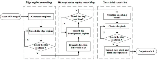
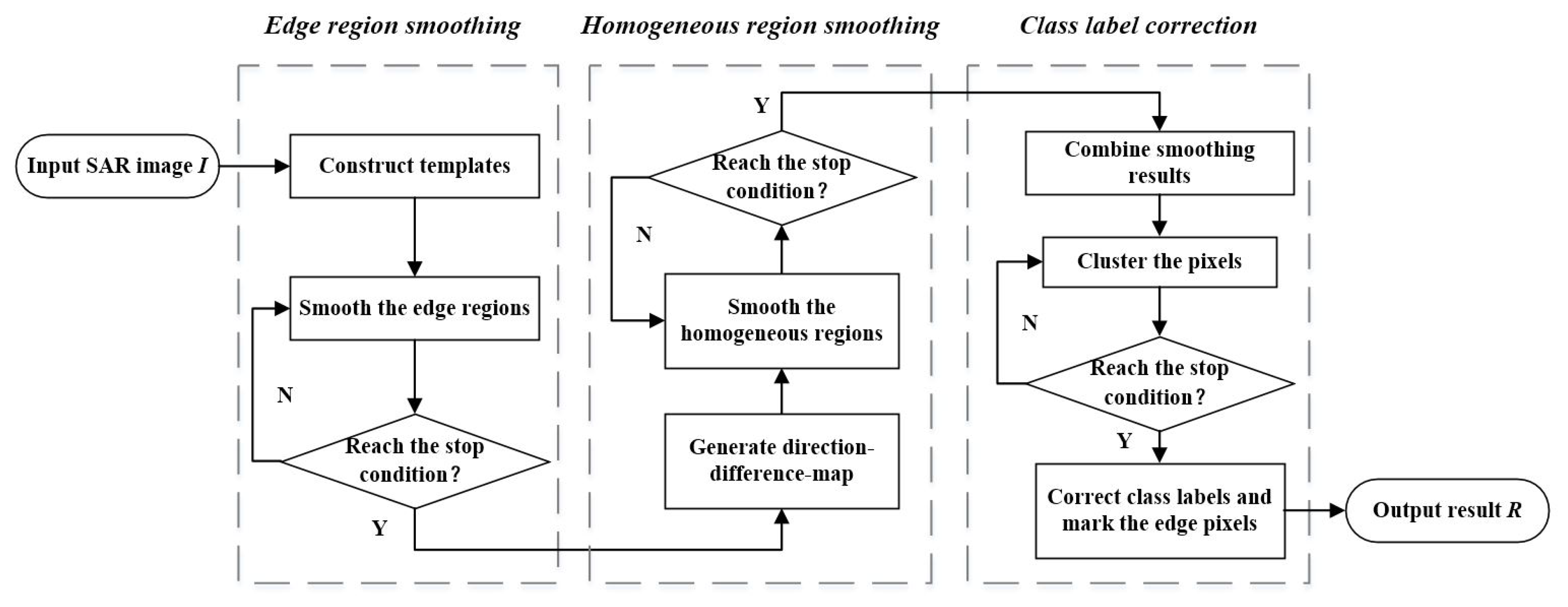
In order to realize this kind of SAR image segmentation more efficiently, a SAR image segmentation method using region smoothing and label correction (RSLC) is proposed in this paper. RSLC uses the region smoothing method to get similar results of spatial information polynomials. A region constraint majority voting algorithm is also used to correct the wrong class labels so as to improve the segmentation accuracy of RSLC. There are usually homogeneous regions and texture regions in SAR images. Homogeneous regions are those regions where the pixel distribution has no specific directionality and the pixel values are close. Texture regions are those regions where the pixel distribution has a specific directionality and the pixel values change according to a certain rule. The texture regions are usually composed of smaller homogeneous regions and edge regions. Edge regions are where the edges of the image are. These regions usually have the largest changes in pixel values and are most prone to segmentation errors. So we deal with the edge regions and the homogeneous regions separately.
RSLC firstly constructs eight direction templates to detect the gradient direction of each coordinate. According to the gradient direction, the corresponding smoothing template is used to smooth the edge regions. Thus, effective edge region smoothing is achieved while preserving the edge information. Better smoothing results can be achieved by performing iterative smoothing operations. The direction results of multiple iterations can be used to calculate the direction-difference map, which indirectly represents the homogeneous regions and edge regions of the image. The value of the direction-difference map is taken as the standard deviation of the Gaussian kernel function to convolve the image. It achieves the smoothing of the image’s homogeneous regions. Then, RSLC combines the results of the two smoothing methods and uses a K-means algorithm to obtain the preliminary segmentation results. RSLC uses the image edge detected by the Canny algorithm as the constraint and uses the image sliding window as the scope to perform a region growth algorithm at each coordinate point. RSLC selects the majority class label as the current point’s class label. Finally, RSLC marks the label of the edge pixel as the label of the most similar pixel in its neighborhoods. Thus, the final segmentation results are obtained.
The main contributions of this paper are:
- (1)
- By detecting the direction of all pixel points in the image and smoothing the image with the corresponding template, the edge regions of the image can be effectively smoothed to reduce the influence of noise. The iterative smoothing process used allows better smoothing results to be obtained.
- (2)
- The direction-difference map of the image is calculated by using the direction of the image detected iteratively. It is used as the standard deviation of the isotropic Gaussian kernel to smooth the homogeneous regions of the image. The process allows the homogeneous regions to be smoothed quickly and the edge regions to be unaffected as much as possible.
- (3)
- The region growth algorithm with an image edge constraint and majority voting are used so that a small number of wrong class labels can be corrected. This processing step has a small time cost in order to achieve better accuracy.
The main structure of this paper is as follows: Section 2 gives the specific implementation steps of the proposed algorithm. Section 3 presents and analyzes the experimental results. Section 4 presents a discussion of the experimental results and the proposed algorithm. Section 5 draws conclusions and suggests further work.
2. The Proposed Method
2.1. Edge Region Smoothing
Solving speckle noise from its mathematical model is complicated, so we mainly solve it from its effect on pixels. The effect of speckle noise is mainly to make the pixel values of the same target fluctuate differently. It leads to the wrong result of many different labels for the same target. For an image denoising task, the original values of the pixels need to be restored as much as possible. However, for an image segmentation task, it is not necessary to restore the original image. As long as the pixels of a target have similar values, they will eventually be assigned the same label. We perform smoothing operation on SAR images with speckle noise to achieve this goal.
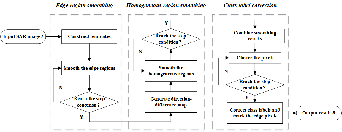
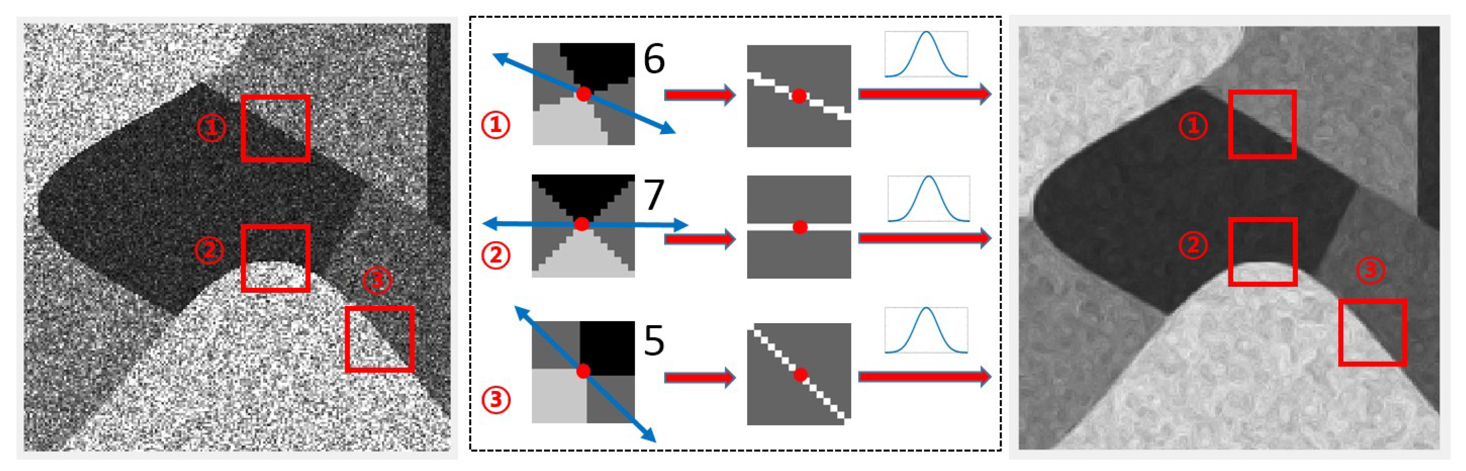
Many image segmentation methods require the special processing of image edges. Because the edges of the image are the junctions of different objects, segmentation errors are most likely to occur. In general, only when the segmentation of the image edge region is done well can the final results have higher segmentation accuracy. Therefore, this paper also deals with the pixels at the edge regions separately. Firstly, it is necessary to reduce the influence of SAR image noise on the premise of preserving image edge information. We do the analysis of the region direction characteristics in the image as shown in Figure 1.
Through the analysis of the common Gaussian filter and mean filter, it is found that the reason why these filters could achieve effective smoothing in the homogeneous regions is that the gray distribution in these regions basically follows the isotropic distribution (see Figure 1a). It exactly conforms to the spatial characteristics of the Gaussian filter and mean filter, so these filters could smooth the region well. However, in the image edge regions (see Figure 1b), the value distribution of pixels presents different characteristics. The distribution of pixel value is still the same in the direction of homogenization, but it changes sharply in the direction of gradient. If the isotropic smoothing method is still used, the pixels in another region with large differences will be added to the calculation, resulting in image edge degradation.
The directional smoothing can be carried out by using the direction characteristic of the edge regions. In order to achieve more simple and effective anisotropic smoothing, the proposed algorithm smoothes edge regions by using the template perpendicular to the gradient direction (see Figure 2c).
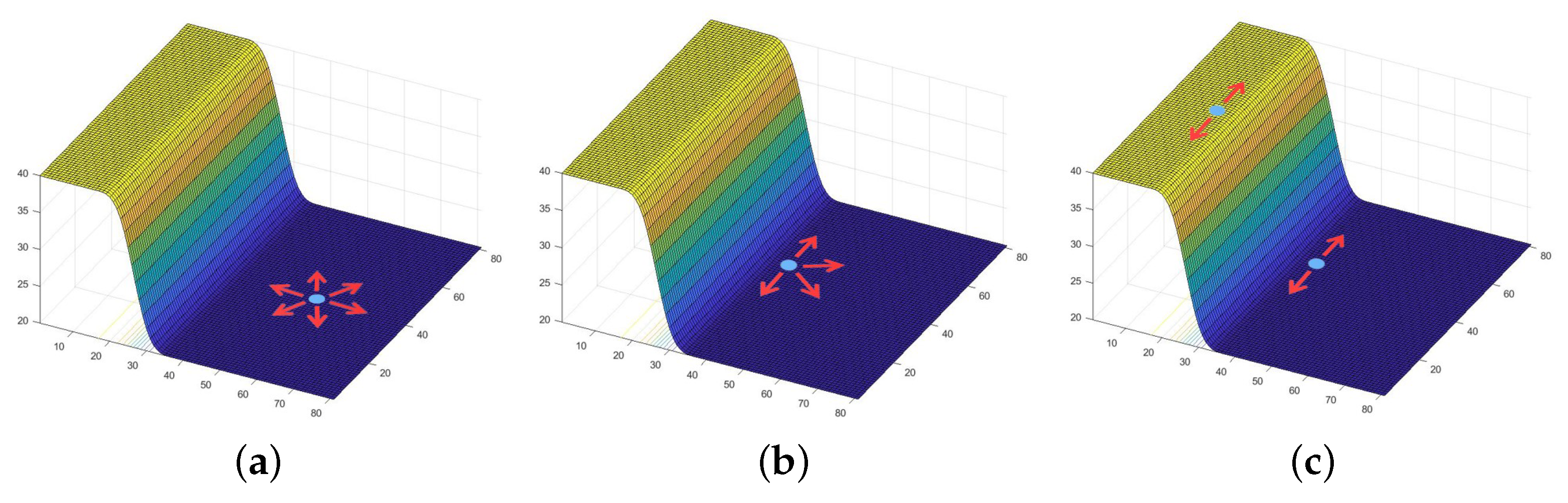
In order to detect different directions in the images, eight direction templates are used for direction detection, as shown in Figure 2a. The corresponding smoothing templates are also built, as shown in Figure 2b. The eight direction templates are built from the first template about the center rotation, as shown in Figure 2c.
The angle difference between the two adjacent templates is 22.5 degrees. Different templates have different response values in different directions, so the direction of corresponding points can be detected. As can be seen from Figure 2a, the directions of all the templates do not cover a 360 degree angle. This is because of the symmetry of the templates. Obviously, the values of the two perfectly symmetric templates are inverse to each other, and the two symmetrical templates give the same smoothing direction so there is no need to double calculate. The construction formula of the first template is as follows:
where is the first direction template, represents the corresponding coordinates in the template, and is the radius value of the direction templates.
In Figure 2c, the value of the white area is 1, the value of the black area is , and the value of the gray area is 0. The regions with values of 1 or are center symmetry, and the mean value of the whole template is 0. The areas of 1 and in the template have an important impact on the smoothness of the results. When region 1 and region overlap at the center of the template, as shown in Figure 2c, the resulting image edges are much smoother. Rotate the first template to get the template in each direction. The formula is as follows:
where is the kth generated template and the function represents counterclockwise rotation; is the first direction template.
The generation of smoothing templates is also based on a similar principle. Firstly, the first smoothing template is generated as follows:
where is the first smoothing template and is the radius of the smoothing template. Use the following formula to generate smooth templates in the other directions:
where is the kth smoothing template and the function represents counterclockwise rotation; is the first smoothing template.
The process of edge region smoothing is shown in Figure 3. From left to right are the original image, the process, and the results, respectively.
As can be seen from Figure 3, different points match different direction templates, and the corresponding smoothing templates are used for the smoothing operation. The process is described in detail below:
Use the direction template to convolve the image in turn, and the direction with the maximum response is the final direction. The calculation formula is as follows:
where D is the direction-index map of the whole image. Its value represents which template is used. is the kth direction template; ∗ represents the convolution operation; I is the original SAR image.
According to the calculated direction index, the corresponding smoothing template is used to smooth the edge regions. The formulas are as follows:
where is the result generated by kth iteration; is the original SAR image; is the smoothing template; M is the maximum iterations; and represents the Gaussian standard deviation. In order to get a better smoothing effect on edge regions, we run the smoothing operator several times.
2.2. Homogeneous Region Smoothing
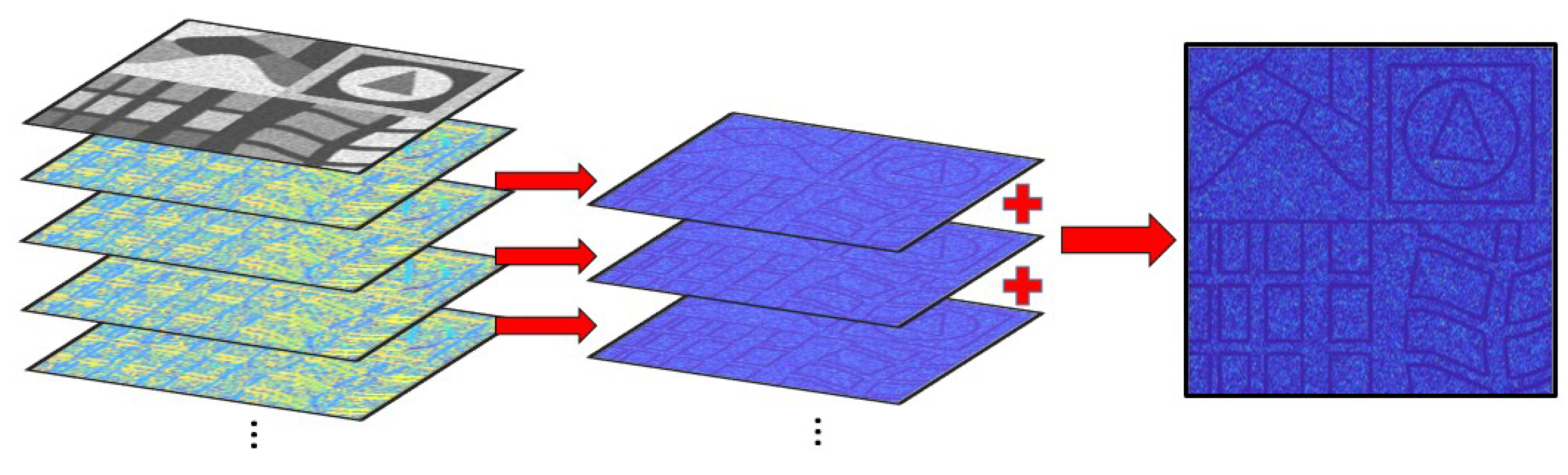
From the principle of edge region smoothing, it can be seen that if the region is not affected by noise, the same regions should keep the same direction during multiple iterations. However, in the actual test, only the edge regions kept the invariance of the detection direction, while the homogeneous regions usually show the different directions during multiple iterations. The reason is that the directions at the edge regions are usually a real gradient, so the gradient can be detected in iterative detections. This leaves the detection results unchanged. While the gradient in the homogeneous regions is usually caused by the noise, there are no real gradients. Since the gray level of these regions usually changes during iteration, so the detection directions also change. By using this property, the homogeneous regions can be distinguished from the edge regions. The calculation formulas are as follows:
where is the kth difference map; and are the th and kth direction-index map, respectively; S is the direction-difference map; represents the operation of taking the modulus. The generation process of the direction-difference map is shown in Figure 4.
In Figure 4, several direction-index maps are used to generate a direction-different map through the Equations (8) and (9). It can be seen from the direction-different map that the homogeneous regions and the edge regions can be clearly distinguished. Some regions have a darker grayscale, indicating that the directions of the regions are consistent. They are usually the edge regions. Other regions are brighter, indicating more variation in direction during the iteration. They are usually homogeneous regions. Therefore, the value of the direction-difference map could be used to determine whether the region is the edge region or the homogeneous region.
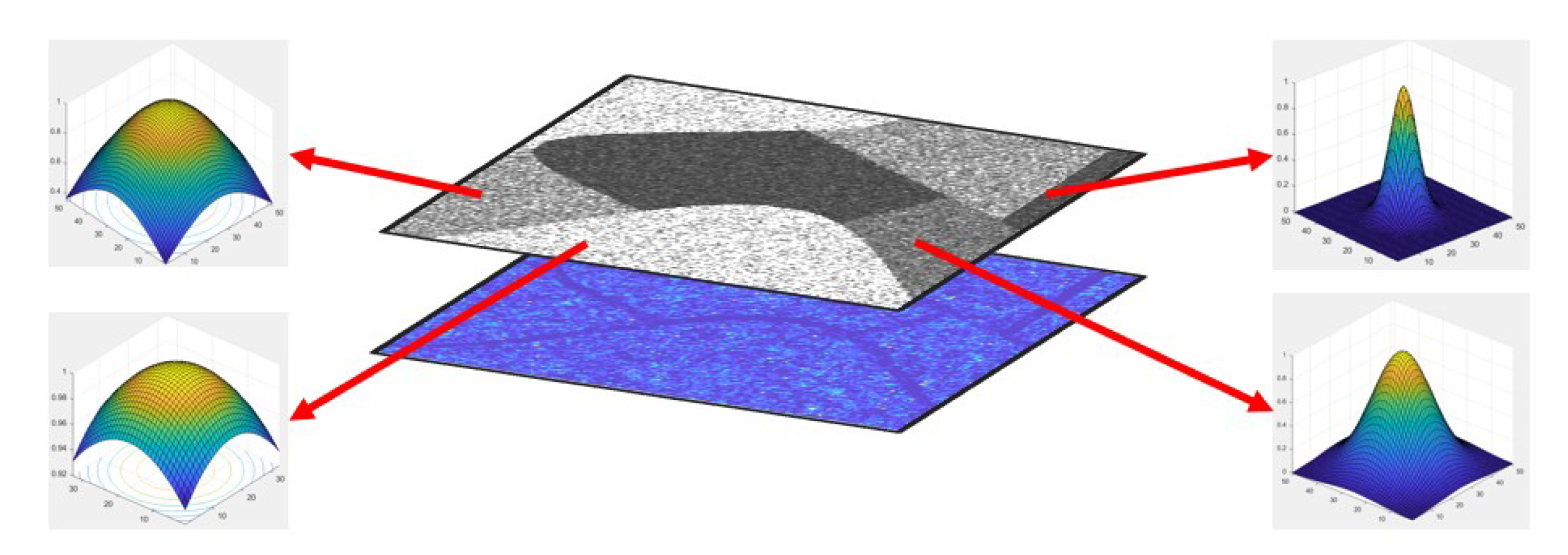
In the process of smoothing the edge regions, the homogeneous regions are partially smoothed. However, because the homogeneous regions are isotropic, the smoothing effect obtained by using the anisotropic smoothing operator is quite general. Considering that the value of the direction-difference map could indirectly distinguish the homogeneous regions and edge regions, the value of the direction-difference map could be used for isotropic smoothing of the homogeneous regions. The smoothing operation is shown in Figure 5.
As shown in Figure 5, the values of the direction-difference map are taken as the variances of the Gaussian kernel function to smooth the homogeneous region. Where the value is large, it is considered to be greatly affected by noise. The smoothing effect is closer to using mean smoothing. Where the value is small, the noise effect is considered small, and a small variance is used to smooth. The smoothing effect is closer to keeping the original value of the pixel. Thus, it achieves smoothing according to the characteristics of different regions. The smoothing process is calculated as follows:
where is the isotropic Gaussian smoothing result; I is the original SAR image; ∗ is the convolution operation; is the Gaussian kernel function; H is the Gaussian normalization term; and S is the direction-difference map.
In order to eliminate the salt-and-pepper noise in the smoothing results, a median filter with the same window size of the Gaussian function can be used for secondary smoothing. Since its window size is fixed, the fast median filtering algorithm can be used to complete the smoothing. The result of the median filtering is denoted as . Iteration can be used to increase the smoothing effect in homogeneous regions.
2.3. Class Label Correction
Edge region smoothing has a better effect on the edge regions. Homogeneous region smoothing has a better effect on the homogeneous regions. Use the following formula to fuse the two results:
where is the fusion result; is the result of homogeneous region smoothing; S is the direction-difference map; and is the result of edge region smoothing.
In the homogeneous regions, because the values of the corresponding direction-difference map are large, more weights are assigned to participate in the fusion. For the edge regions, the values of the corresponding direction-difference map are small, so smaller weights are assigned to participate in the fusion. After the fusion operation, the smoothing results of the whole image are obtained. Regarding the smoothing results as the approximate results of the spatial information polynomials, a K-means clustering algorithm is used to get the preliminary segmentation results and denoted them as the symbol L.
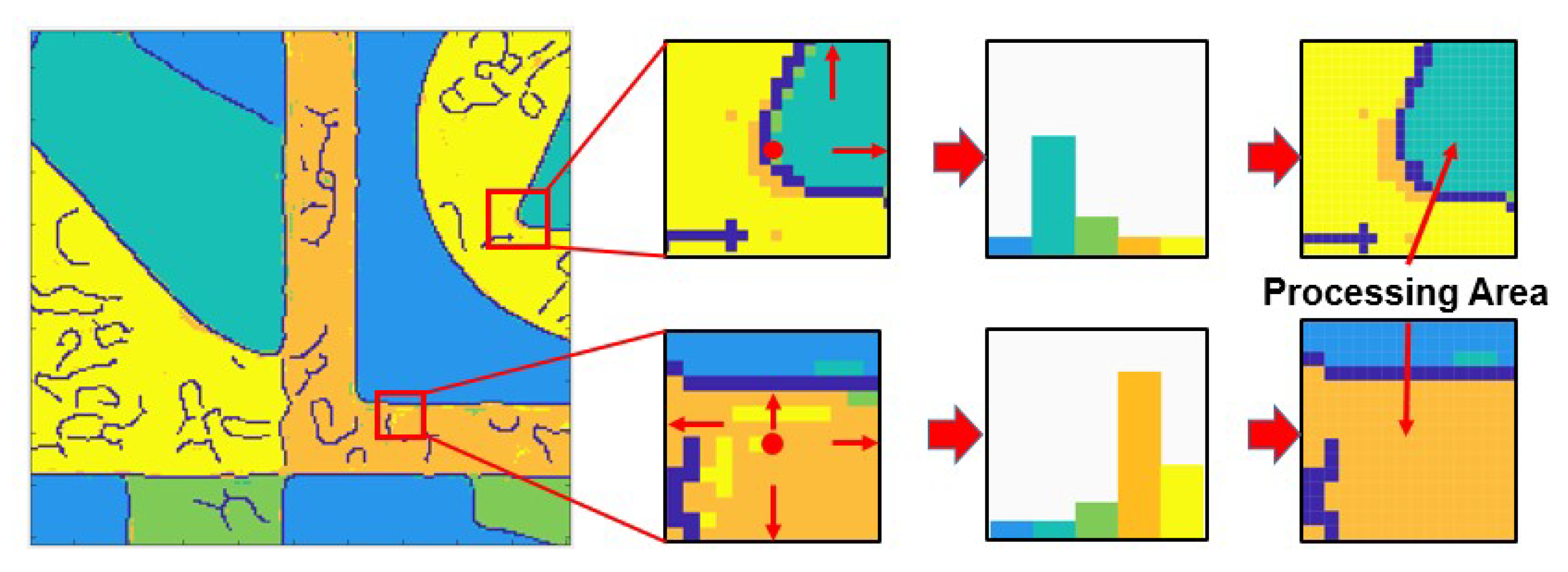
Through the observation and analysis of the clustering results, we found that due to slight edge degradation, a small number of pixels in the edge regions have class label errors. These errors can be corrected in some way. In image edge detection, usually only real targets have completely surrounded edges, while the error targets do not. This difference can be used for error class label correction.
In the process of class label correction, it is necessary to ensure that the edges form a closed space, as much as possible, to obtain a better correction effect. Fortunately, the Canny algorithm will connect the edge lines when performing edge detection, which can improve the closedness of the space surrounded by the edges. In addition, the Canny algorithm is simple and fast to implement, which can guarantee the efficiency of the proposed algorithm. Because it is susceptible to noise interference, it cannot be used directly in the original SAR image. Since the previous part has greatly reduced the influence of noise, the Canny algorithm can be effectively used to extract the image edge. In this paper, the adaptive Canny algorithm function provided in the software Matlab2018 is used for edge extraction. The result of image edge detection is recorded as .
Then, the following formula is used to mark the image edge in the clustering results:
where is the label-map marked edge pixels; is the image edge map; and L is the result map of K-means clustering.
Then, the majority voting method is used to correct the wrong class labels. The process is shown in Figure 6.
Using a fixed window to slide through the image, we regard the image edges as the constraint to perform the region growth algorithm in each window and modify one class label of the center pixel each time. During the performing of the region growth algorithm, the number of each label is counted and the class label with the largest number becomes the final class label. The calculation formula is as follows:
where is the corrected result; represents the four-neighborhood region growth operation; W is the size of the slide window; and is the image label map after marked edge pixels.
As can be seen from Figure 6, under the constraint of the image edge, using region growth for class label correction will not affect other normal class labels, while the wrong pixel labels can be effectively corrected. Finally, it is necessary to assign the class label of the edge pixels. The calculation formula is as follows:
where R is the final segmentation result; is the fusion result; and represents the eight neighborhoods. The formula is to mark the class label of the edge pixels as that of the most similar pixel in the neighborhoods. The specific execution steps of the proposed algorithm are shown in the flowchart in Figure 7.
3. Experimental Setup and Results
3.1. Experimental Images
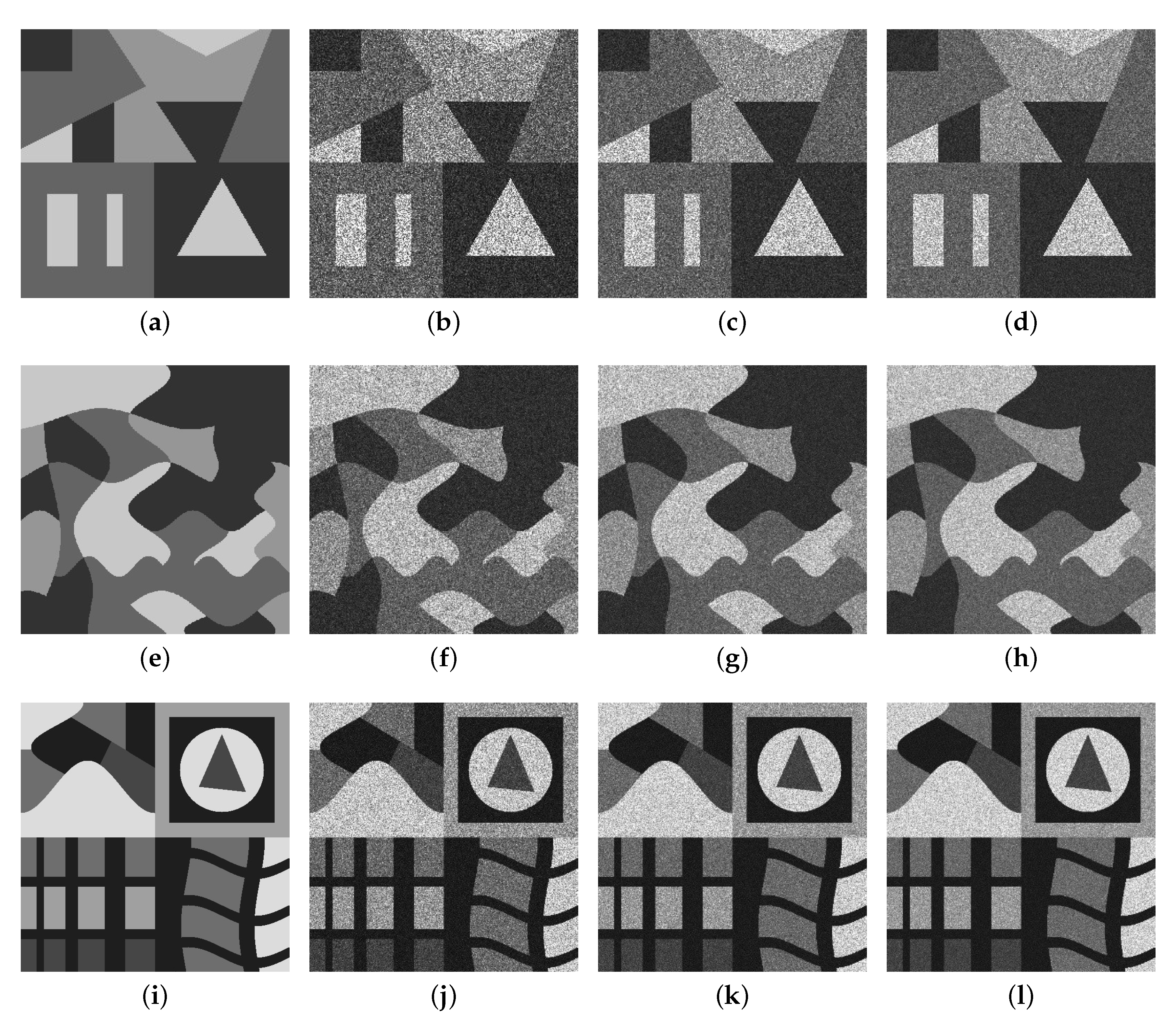
In order to verify the effectiveness of the proposed algorithm for SAR image segmentation, simulated SAR images and real SAR images were used for experimental verification. Three groups of simulated SAR images are shown in Figure 8.
Figure 8a–d are the original clean SI1 image and the 2-, 4-, and 6-look simulated SI1 image, respectively. There are four types of targets with gray values of 50, 100, 150, and 200. The size of the image is 256 × 256. Figure 8e–h are the original clean SI2 image and the 2-, 4-, and 6-look simulated SI2 image, respectively. There are also four types of targets with grayscale values of 50, 100, 150, and 200. The size of the image is 384 × 384. Figure 8i–l show the original clean SI3 image and the 2-, 4-, and 6-look simulated SI3 image, respectively. There are five types of targets with grayscale values of 50, 90, 130, 170, and 210. The image size is 512 × 512. Three groups of simulated SAR images have different line characteristics and scale sizes, which could test the processing ability of the algorithms for different types and sizes.
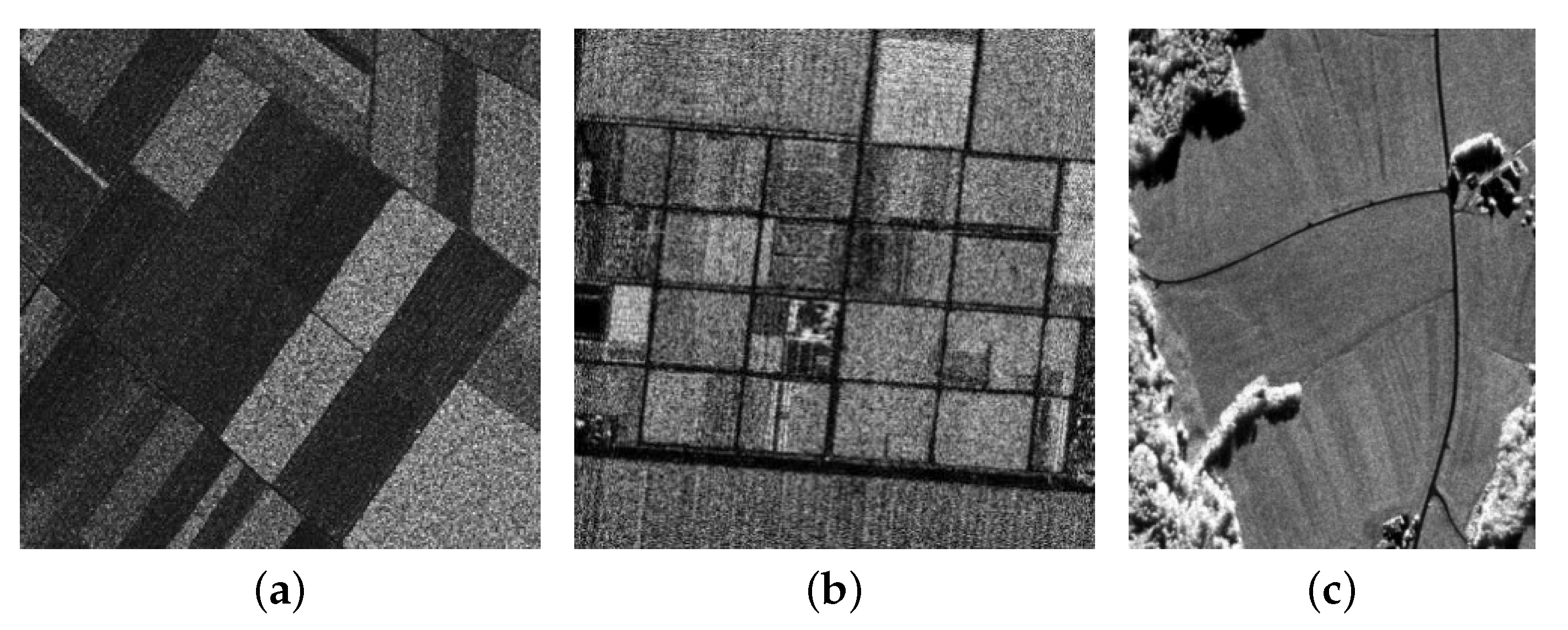
We also set up a group of experiments containing three real SAR images: Noerdlinger, Maricopa, and Traunstein, as shown in Figure 9.
Noerdlinger in Figure 9a was taken in the middle of the Swabian Jura mountains in southwest Germany. The image size is 256 × 256 and can be divided into four different farmland areas. Maricopa in Figure 9b was taken at the Maricopa agricultural center near Arizona, in the United States. The image size is 350 × 350 and can be divided into four different areas including water and different agricultural fields. Traunstein in Figure 9c was taken in Bavaria, Germany. The image size is 1001 × 779 and can be divided into three different areas including forest, farmland, and shadow. Among them, Noerdlinger and Maricopa image have large amounts of noise, while the Traunstein image is relatively less affected by noise.
3.2. The Compared Algorithms and Evaluation Indicators
In this paper, five unsupervised SAR image segmentation algorithms are used as comparative experiments to verify the effectiveness of the proposed algorithm. They are NSFCM [1], ILKFCM [28], FKPFCM [29], CKSFCM [30], and ALFCM [31]. In the experiment, two quantitative indexes are used for comparison: the segmentation accuracy rate (%) and the time consumption (s). The time consumption of the algorithm is obtained directly through the program timing, and the segmentation accuracy is calculated as follows:
where is the segmentation accuracy, whose value is the number of correct classifications divided by the number of all pixels; C is the number of classes; R is the final segmentation result; and is the real segmentation result.
3.3. Parameter Sensitivity Analysis
The experiments were carried out on an Intel Core i5-6500m 3.2ghz, 8G memory and Win 7 64-bit operating system, using the software Matlab2018b.
The proposed algorithm needs to set several groups of parameters before running, among which several parameters have fixed values. In the experiments, the diameter of the direction templates is set as 7, the diameter of the smooth templates is set as 5, and the diameter of Gaussian filters is set as 5. There are several other parameters that need to be selected from a wide range: edge region smoothing iteration times , homogeneous region smoothing iteration times , and majority voting sliding window W.
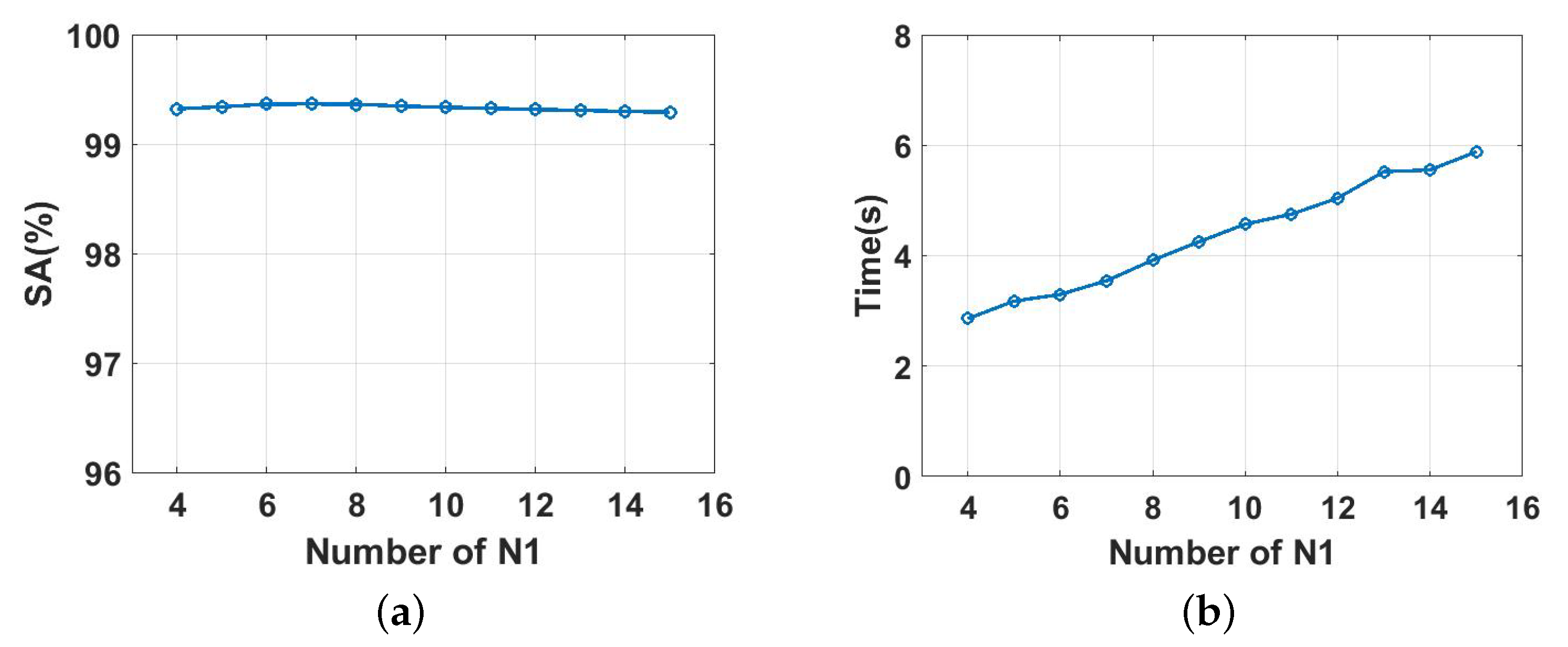
First, we tested the effect of the parameter on the results. We set its value from 4 to 15 with a step of 1. During the test, parameter was set as 2 and parameter W was set as 21. The experimental results are shown in Figure 10.
It can be seen from Figure 10a that parameter only has a small impact on the accuracy of the results. The accuracy is always kept above 99%, and the highest accuracy is achieved when is around 6. As can be seen from Figure 10b, the time consumed by the algorithm increases significantly with the increase of parameter . The main reason is that the increase of this parameter makes the edge region smoothing process take more time. Consider that in the above analysis, the value of can be selected from 4 to 7.
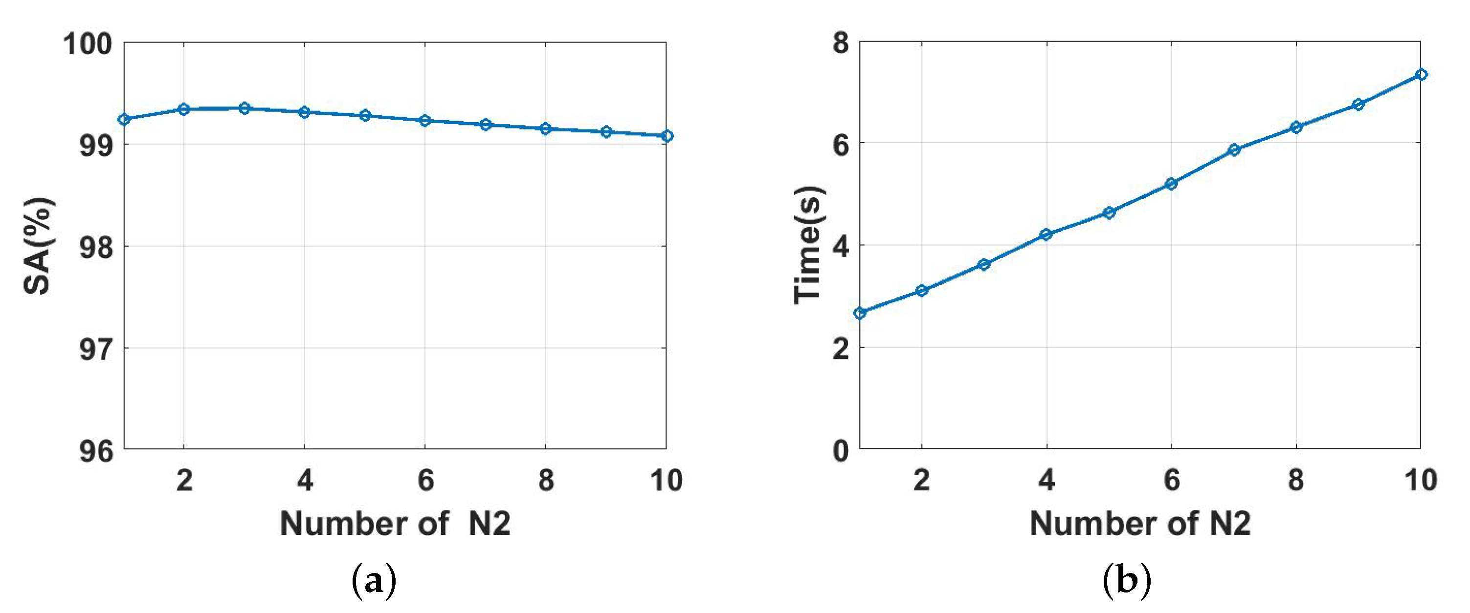
Next, we tested the effect of the parameter on the results. We set its value from 1 to 10 with a step of 1. During the test, parameter was set as 5 and parameter W was set as 21. The experimental results are shown in Figure 11.
As can be seen from Figure 11a, with the increase in iteration times, the accuracy rate increases slightly at first and then decreases slowly. The reason is that when is small, an increase of its value can obtain a better smoothing result. However, after reaching the optimal value, the further increase of ’s value will lead to the degradation of the edge region and increase the segmentation error rate. As can be seen from Figure 11b, with the increase of , the time consumption also increases significantly, mainly because more time is taken to smooth the homogeneous region. Consider that in the above analysis, the value of can be selected from 1 to 4.
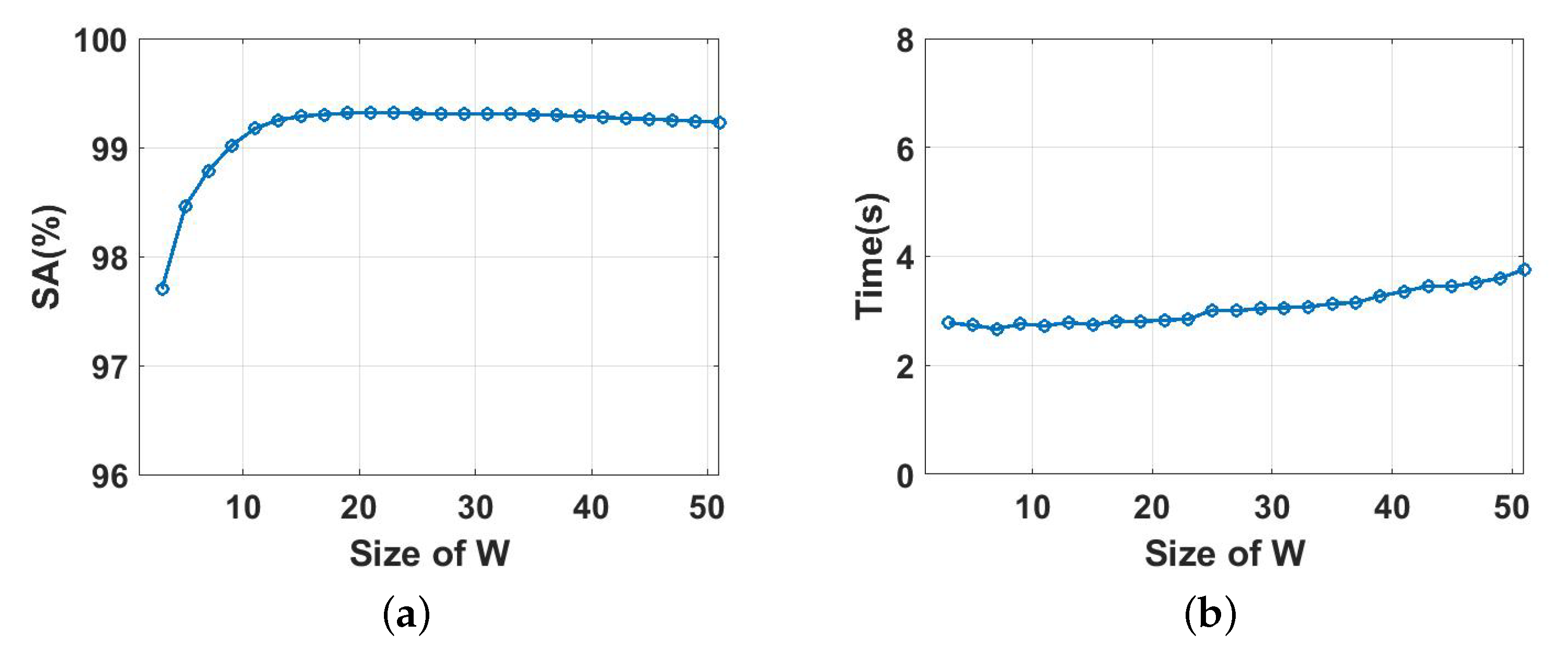
Next, we tested the effect of parameter W on the results. We set its value from 3 to 51 with a step of 2. During the test, was set as 5 and was set as 2. The experimental results are shown in Figure 12.
As can be seen from the results in Figure 12a, with the increase of W, the accuracy increases significantly at first and then decreases slightly. The reason is that the increase of W at the beginning increases the range of correction, which leads to an increase in accuracy. However, if W continually increases, part of the correct labels will be marked incorrectly, which will increase the error rate. As can be seen from Figure 12b, with the increase of W, the time consumption increases only slightly and not significantly. The reason is that for the region completely surrounded by the edges, the search space will not increase even if parameter W increases. For some regions that are not completely surrounded by the edges, only a small time cost will be added. Consider that in the above analysis, the value of parameter W can be selected from 15 to 35.
3.4. Results and Analysis
This section may be divided by subheadings. It should provide a concise and precise description of the experimental results, their interpretation as well as the experimental conclusions that can be drawn.
3.4.1. Results and Analysis of SI1
The experimental results of the proposed algorithm and the comparison algorithm on the SI1 image are shown in Table 1, including the segmentation accuracy (%) and time consumption (s).
From the results in Table 1, it can be seen that the accuracy of all the algorithms is over 90%. Among them, the accuracy of the CKSFCM and ALFCM algorithms vary greatly with the change of noise, indicating that they are sensitive to noise. While the accuracy of ILKFCM, NSFCM, FKPFCM, and the proposed algorithm only have a small change, indicating that they are robust to noise. Moreover, the proposed algorithm achieves the highest accuracy on three images with noise of different intensity, which indicates its effectiveness. It can also be seen that the CKSFCM algorithm takes the longest time, and ALFCM, ILKFCM, NSFCM, and FKPFCM take less time but still more than the proposed algorithm. In this group of experiments, both the accuracy and the time consumption of the proposed algorithm are optimized.
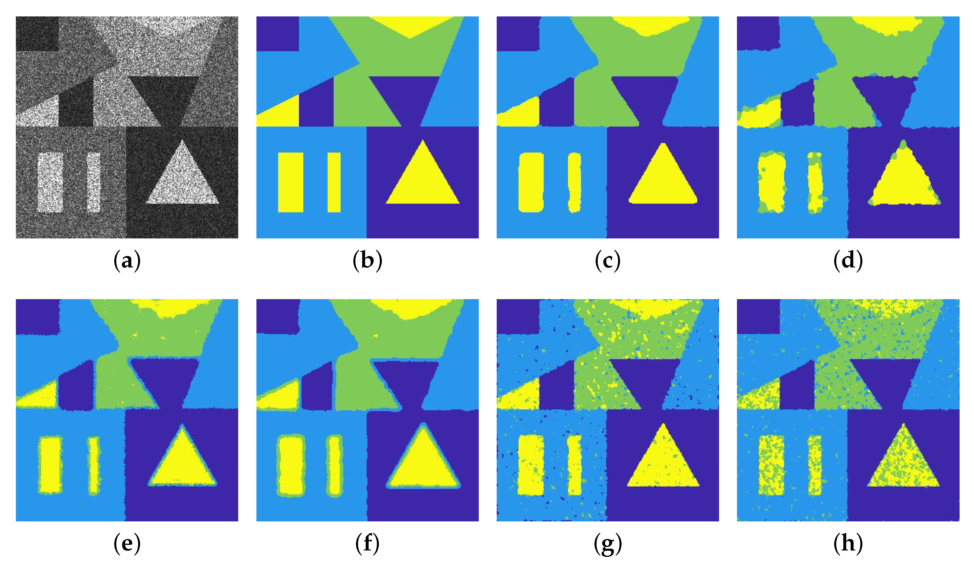
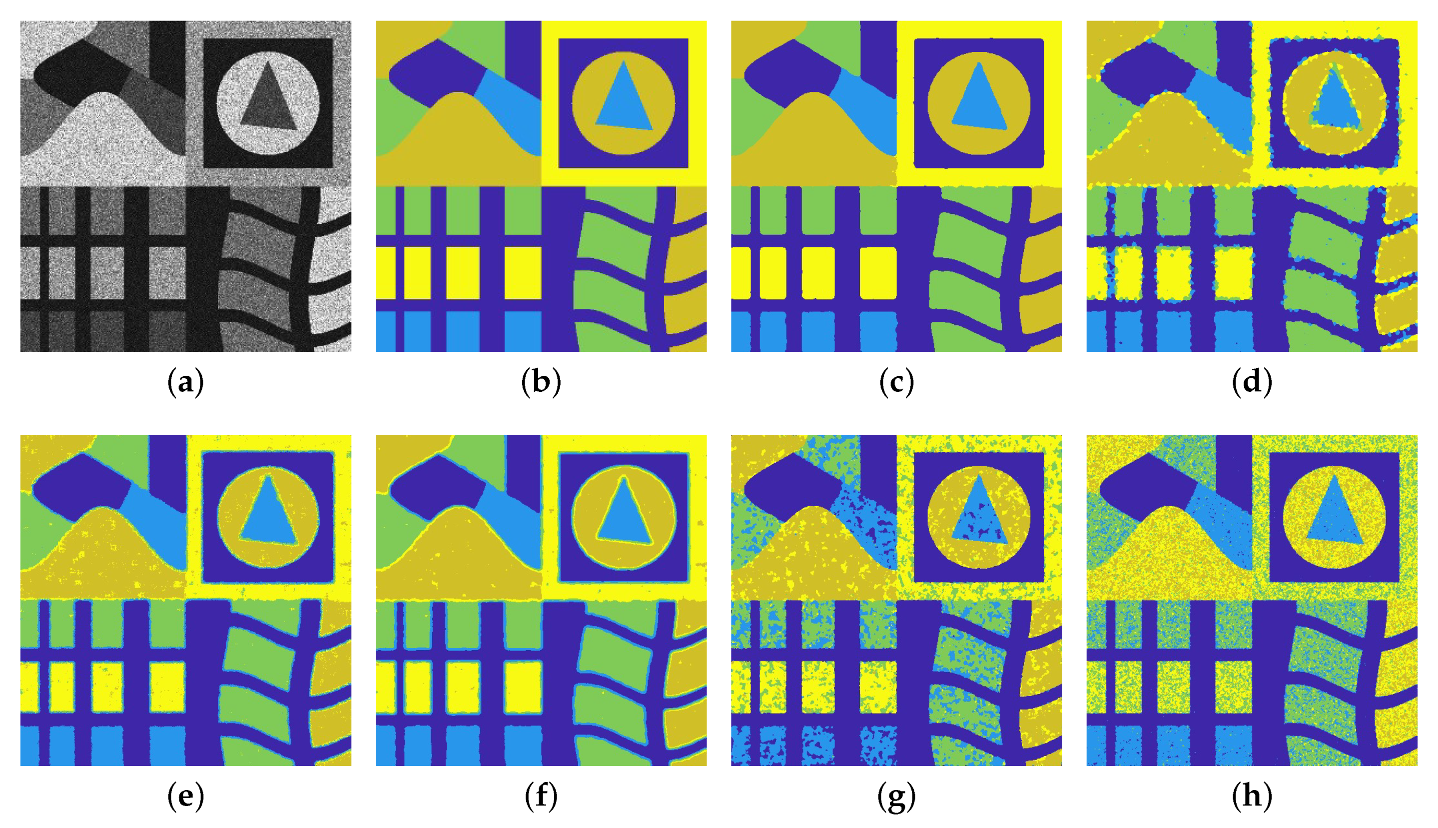
The experimental results of each algorithm on the 2-look simulated SI1 image are as shown in Figure 13.
From the segmentation results in Figure 13, it can be intuitively seen that the results of the ALFCM and CKSFCM algorithms (see Figure 13g,h) have a large number of noise points caused by wrong labeling, indicating that the robustness of these two algorithms to noise is not good. The NSFCM and ILKFCM algorithms (see Figure 13e,f) can better segment different regions, but it can be seen that there are obvious errors in the junction of different targets. The result of the FKPFCM algorithm (see Figure 13d) is relatively clean on the whole, but the segmentation edge is not smooth and there are also many errors at the edges of different targets. The results of the proposed algorithm (see Figure 13c) are much cleaner and noiseless, with clear smooth edges and fewer errors.
3.4.2. Results and Analysis of SI2
The experimental results of the proposed algorithm and the comparison algorithms on the SI2 image are shown in Table 2, including the segmentation accuracy (%) and time consumption (s).
As can be seen from Table 2, the accuracy of the CKSFCM and ALFCM algorithms still varies greatly under different noises. This again shows that the two algorithms are not robust to noise. The accuracy of the ILKFCM, NSFCM, and FKPFCM algorithms are still relatively stable. The accuracy of the proposed algorithm is kept above 99%, which is not only accurate but also robust to noise. It can be seen that the time consumption of each algorithm increases obviously with the increase in image size. The NSFCM and FKPFCM algorithms consistently maintain low time consumption. The proposed algorithm also maintains low time consumption under different level of noise, and the time consumption is significantly lower than that of the comparison algorithms.
The experimental results of each algorithm on the 2-look simulated SI2 image are shown in Figure 14. As can be seen from the intuitive experimental results in Figure 14, the experimental results of the ALFCM and CKSFCM algorithms (see Figure 14g,h) still have many false noise points. The results of the NSFCM and ILKFCM algorithms (see Figure 14e,f) are relatively clean and accurate, but careful observation shows incorrect segmentation at the junction of different targets. The result of the FKPFCM algorithm (see Figure 14d) has a few false segmentation noise points, and there are many false segmentation points at the edges, which leads to the unsmoothness of the segmentation edge. The result of the proposed algorithm (see Figure 14c) is relatively clean, with no obvious noise misclassification. The different targets are well separated and the edges are smooth and clear.
However, the proposed method also has some shortcomings: It can be seen that the tail of the yellow target in the image is not segmented correctly, while the ALFCM and CKSFCM algorithms correctly segment the target (see Figure 14g,h). The main reason is that the width of the smoothing template used in the experiment is 5, but the width of this yellow tail target is smaller than this value. Therefore, the pixel value of this area will be affected by the surrounding pixels during the smoothing process, which will cause the subsequent clustering process to be mislabeled. In addition, the class label correction process also increases the number of error labels. Therefore, the proposed algorithm will be limited by the minimum width of the segmentation target. Thus, the proposed algorithm will be limited by the minimum width of the segmentation target.
3.4.3. Results and Analysis of SI3
The experimental results of the proposed algorithm and the comparison algorithms on the SI3 image are shown in Table 3.
As can be seen from Table 3, for the SI3 image with a more complex structure, the accuracy of the comparison algorithms decreases significantly. The accuracy of the CKSFCM and ALFCM fluctuates greatly and shows that noise has a great influence on these two algorithms. The accuracy of the IKLFCM, NSFCM, and FKPFCM vary less than 3%. The segmentation accuracy of the proposed algorithm is still higher than 99%, with obvious advantages. With the increase in experimental image size, it can be seen that CKSFCM, ALFCM, and ILKFCM are more time-consuming than the other algorithms. The time consumption of NSFCM and FKPFCM remains low. The proposed algorithm still gets the lowest time consumption and has a great advantage compared with other algorithms.
The experimental results on the 2-look simulated SI3 image are shown in Figure 15. As can be seen from the intuitive experimental results in Figure 15, the results of the ALFCM and CKSFCM algorithms (see Figure 15g,h) become more serious. The possible reason is that the gap between SI3 classes becomes smaller, which leads to a greater influence of noise on real data. The results of the NSFCM and ILKFCM algorithms (see Figure 15e,f) generally segment the complete targets, but there are also many false noise points. By zooming in, we can still see that there are some errors at the edges of the targets. The result of the FKPFCM algorithm (see Figure 15d) shows the wrong labeling block at the segmentation edges. These errors also lead to unsmooth segmentation edges. The results of the proposed algorithm ()see Figure 15c) are clearly segmented, with no obvious noise labels. The segmentation edges are complete and smooth, and the whole result is much closer to the ground truth.
3.4.4. Results and Analysis on Real SAR Images
The experimental results of the proposed algorithm and the comparison algorithms on real SAR images are shown in Table 4, including the experimental accuracy (%) and time consumption (s).
As can be seen from the experimental data in Table 4, for the Noerdlinger and Maricopa images with high noise, the proposed algorithm achieves the highest accuracy. From the perspective of time consumption, CKSFCM, ALFCM, and ILKFCM take significantly longer than the other algorithms. The NSFCM and FKPFCM algorithms take less time, but the proposed algorithm consumes the shortest amount of time. In the Traunstein image with low noise, the accuracy of the proposed algorithm is 89.69%, slightly lower than that of ILKFCM’s 89.92% and thus ranking second. But the proposed algorithm only consumes 5.43 s, far less than the 1001.83 s of the ILKFCM algorithm.
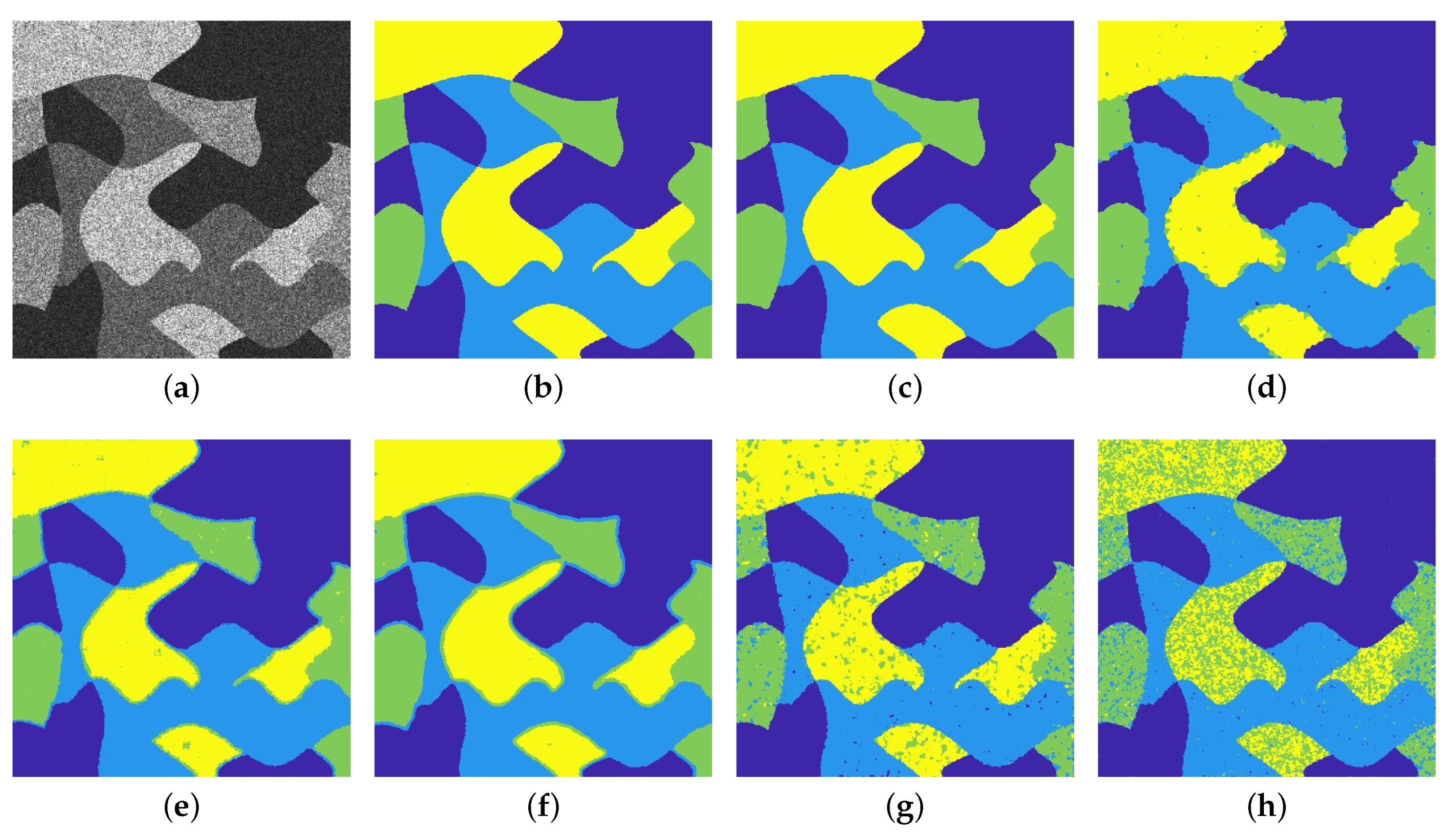
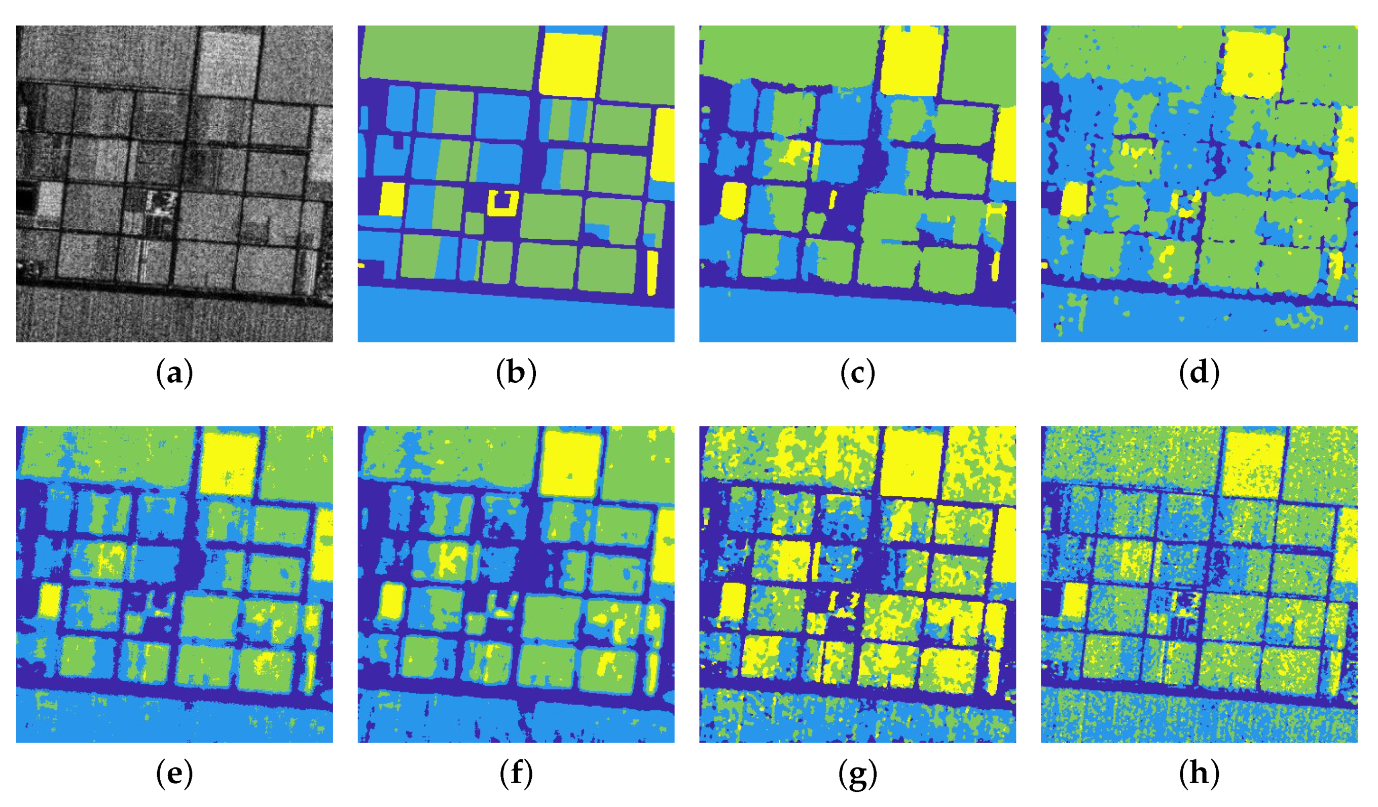
The experimental results of each algorithm on Noerdlinger images are shown in Figure 16.
As can be seen from Figure 16, the false noise points in the results of ALFCM and CKSFCM (see Figure 16d,g,h) are serious, which affects the accurate segmentation of different targets. The results of the NSFCM and ILKFCM algorithms (see Figure 16e,f) have less noise, but there are pixels misclassified into wrong classes at the edges. The FKPFCM algorithm (see Figure 16d) shows many obvious segmentation errors at the edges, resulting in an unsatisfactory result. The result of the proposed algorithm (see Figure 16c) is much cleaner, with no obvious noise error, and the segmentation edges are relatively smooth.
However, we can also see the shortcomings of the proposed algorithm: the thin line in the middle of the yellow area is missing (see Figure 16c), while it is better recognized in the results of the NSFCM, ALFCM, and CKSFCM algorithms (see Figure 16e,g,h). One of the reasons is that this thin line is actually only 1–2 pixels wide but the template used in the smoothing process is 5 pixels wide, which will cause the degradation of the thin line. In addition, only the labels of objects surrounded by closed edges can be corrected during the class correction process. However, the outer edge pixels of the thin line target cannot form a closed space, so they are easily marked as other labels during the class label correction process. Therefore, when using the proposed algorithm for SAR image segmentation, it is best to ensure that the minimum target width is greater than the width of the smoothing template.
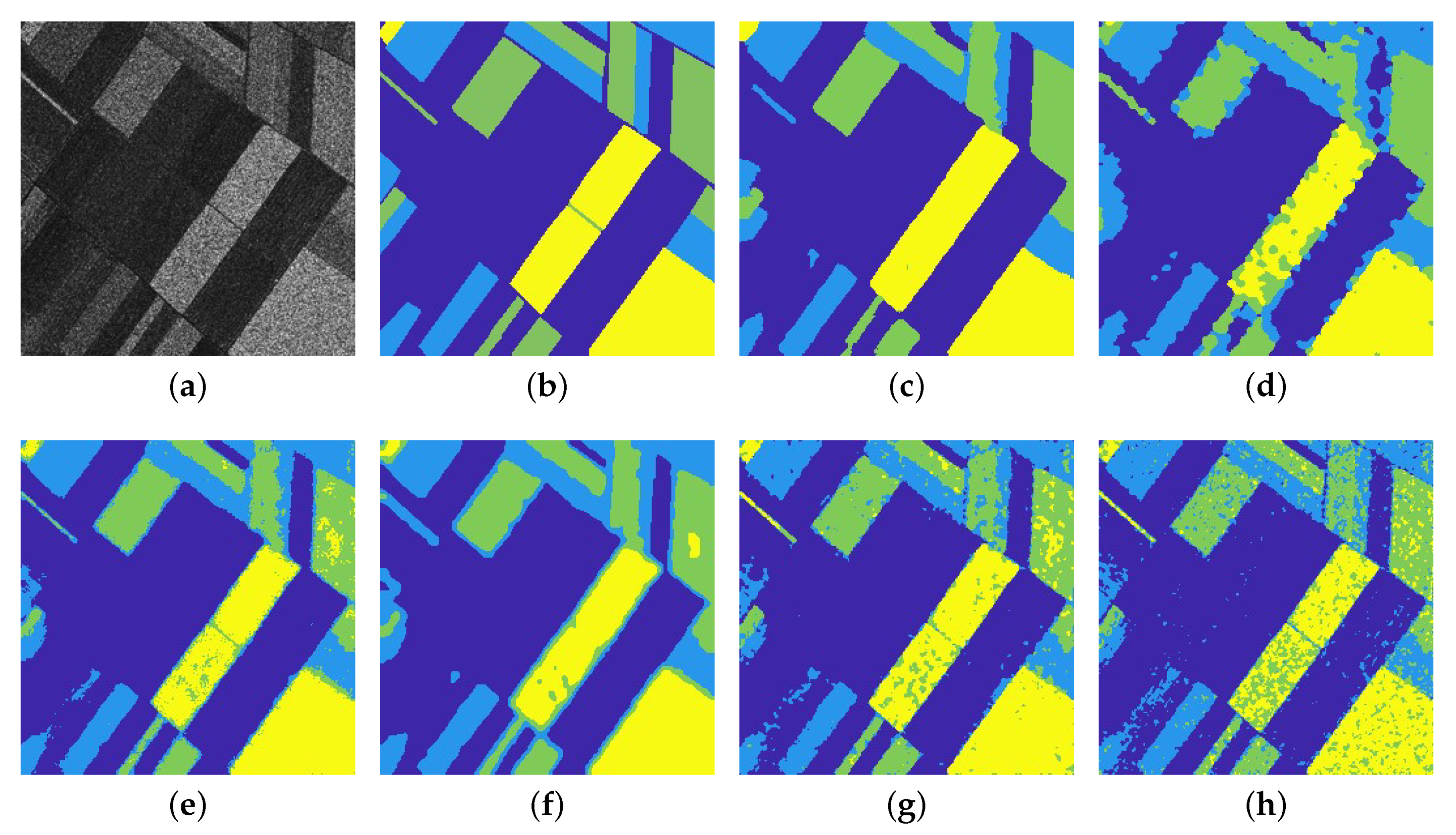
The experimental results of each algorithm on the Maricopa image are shown in Figure 17. As can be seen from the intuitive results in Figure 17, the experimental results of the Maricopa algorithms are greatly different due to the large noise in the experimental images. Among them, the results of ALFCM and CKSFCM (see Figure 17g,h) are sensitive to noise, so there are many noise points and errors in the results. The results of NSFCM and ILKFCM (see Figure 17e,f) are basically good at image segmentation, but there are also many wrong noise labels. The result of the FKPFCM algorithm (see Figure 17d) does not effectively preserve the roads in the farmland, and the target edges was not straight. The result of the proposed algorithm (see Figure 17c) is much smoother, with clearer segmentation edges and better retention of roads in farmland.
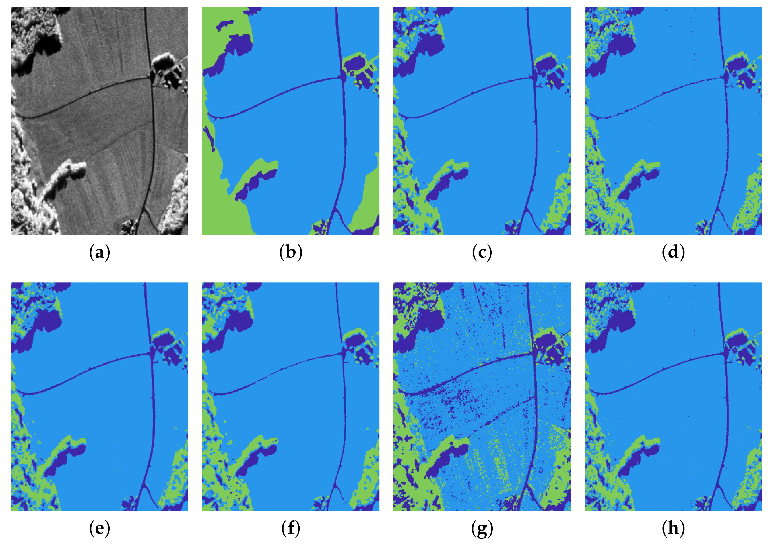
The experimental results of each algorithm on the Traunstein image are shown in Figure 18.
As can be seen from the intuitive experimental results in Figure 18, all algorithms have a good segmentation result for the low-noise image. Among them, the result of the ALFCM algorithm (see Figure 18g) has relatively obvious error segmentation points and is slightly worse. Other algorithms can effectively segment the roads, plains, and woods, and their edges are relatively clear. Visually, the difference between them is not too large, indicating that these algorithms all show good segmentation performance for low-noise images.
3.4.5. Results and Analysis on a Large Data Set
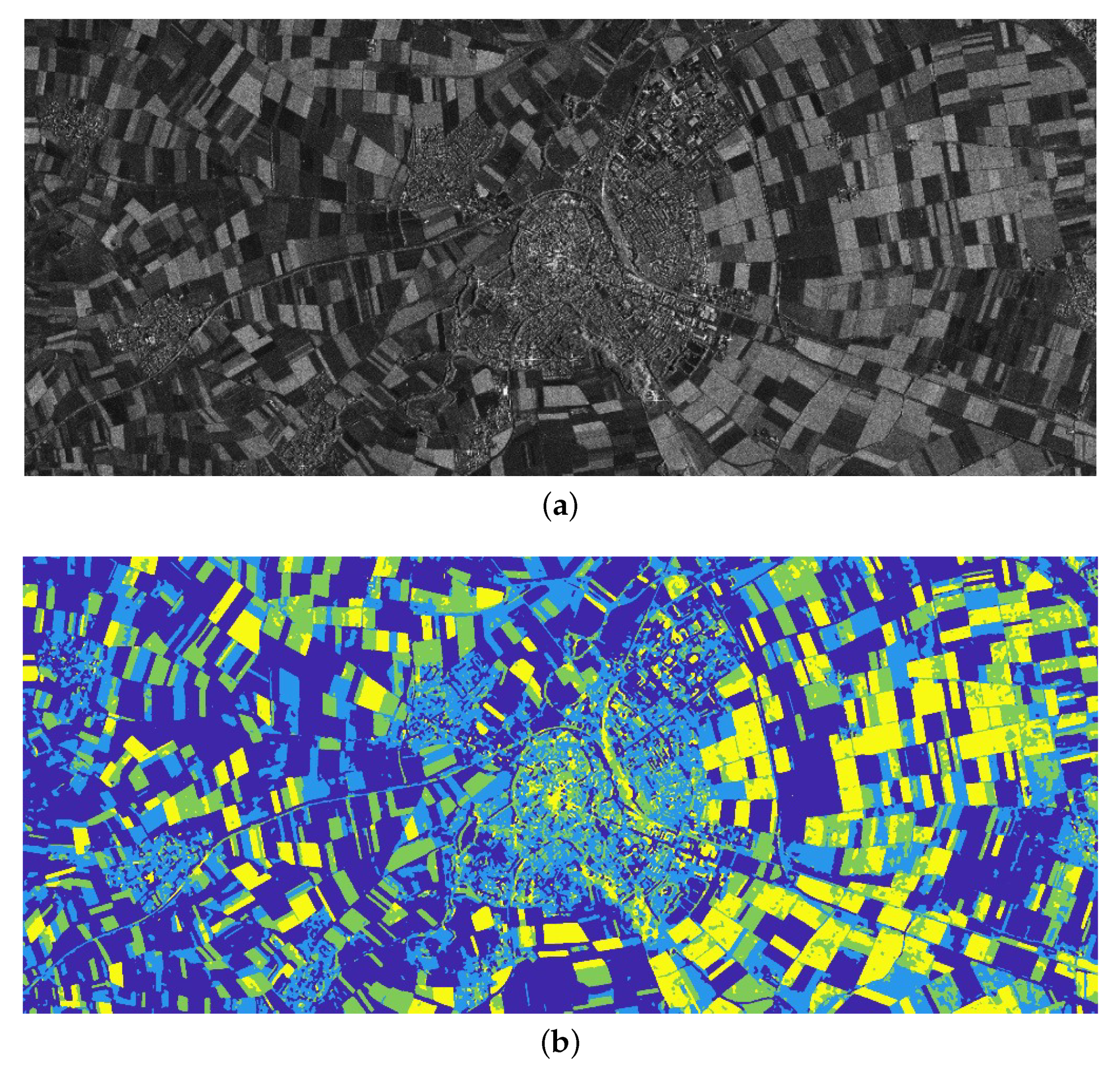
In order to test the performance of the proposed algorithm on a large data set, we used a real SAR image of size 3543×1506 for testing. The experimental images and results are shown in Figure 19.
It can be seen from Figure 19a that this is a larger SAR image, which contains some building targets, a large amount of farmland and roads of different sizes. Because there are so many targets in the image, it is very difficult to mark the ground truth of the image, and the marking process will take a lot of time. It can be seen from Figure 19b that the proposed algorithm performs well in the segmentation experiment of large SAR images. There is less noise in the result, and the segmentation boundary is smooth. More importantly, it only took about 118 s to get this segmentation result. For the segmentation of large images, this time consumption is completely acceptable. It shows that the proposed algorithm is also suitable for the segmentation of large SAR images.
4. Discussion
The robustness of ALFCM and CKSFCM to noise is not good, so the results vary a lot under different levels of noise. In the segmentation results of these two algorithms, there is usually obvious noise, which leads to the decrease of accuracy. The accuracy of FKPFCM, NSFCM, and ILKFCM does not change much under different noise intensities. They are more robust to noise. The problem with these algorithms is that more pixel segmentation errors are prone to occur at the edges, resulting in a decrease in accuracy. The proposed algorithm can maintain high accuracy under different levels of noise, and the edges of the results are much clearer and smoother. There is almost no noise in the results of the proposed algorithm. But the proposed method has an insufficient segmentation ability for small targets, such as thin-line targets. When using the proposed algorithm, it is best to ensure that the width of the target is smaller than the width of the smooth template. Or, the width of the smoothing template and the parameter W of the class label correction process can be appropriately reduced to better detect small targets. In terms of time consumption, CKSFCM, ALFCM, and ILKFCM take the longest time. The time consumption of NSFCM and FKPFCM is relatively short, but the proposed algorithm maintains the shortest time consumption in all experiments. Therefore, considering the segmentation accuracy and time consumption, the proposed algorithm has obvious advantages over the comparison algorithms, indicating the effectiveness of the proposed algorithm.
Through experiments, we found that there are two important parameters for the segmentation of small targets in an image: one is the width of the smoothing template, and the other is the parameter W in the class label correction process. In order to ensure a smooth effect without affecting small-target segmentation, a smooth template with a width of 5 was used in the experiments. Only when the minimum width of the target is greater than this value can smoothing be performed efficiently without degrading edges. Although the template with a width of 5 is already very small, a smaller target may still affect the segmentation effect. Therefore, the proposed algorithm may be more suitable for SAR image segmentation where the minimum target width is greater than 5 pixels. In addition, the parameter W will further affect the result. Because the edges of small targets are more easily degraded due to smoothing, the edge detection algorithm cannot effectively extract a closed space. In this case, a value of W that is too large will cause the correct labels rarely existing in small targets to be modified, leading to a further decrease in accuracy. Therefore, when there is a small-width target in the image, choosing a smaller W parameter is a better choice.
Since most of the processing in the proposed algorithm is serial, the previously used free memory can be used again in later steps. Therefore, as long as we know the value when the memory demand is greatest, we can know the memory demand of the algorithm. We found that the memory requirements were greatest when generating the direction-difference map. Since it is only necessary to have adjacent direction maps to perform calculations, only memory twice the size of the image is needed to store intermediate results. It also requires extra memory twice the image size to store the direction-difference map and results of the edge region smoothing. Therefore, a total of four times the memory size of the image is required. The direction-detection process needs to store the direction map, response results, and detection templates. The edge region smoothing process needs to store the direction map, smoothing results, and smoothing templates. The homogeneous region smoothing process needs to store the direction-difference map and the smoothing results. However, the memory requirements of these processes are less than four times image size memory. Edge detection, k-means clustering, and majority voting are performed sequentially. Each of them uses less space than the above-mentioned memory. Therefore, when the memory usage is the largest, four times the image size is required. Considering the storage of the original image and some other small intermediate variables, the proposed algorithm requires at least five to six times the memory size of the image.
5. Conclusions
A SAR image segmentation method using region smoothing and label correction is proposed in this paper. In the first step of the algorithm, the direction templates and the corresponding smoothing templates are used to smooth the edge regions. Experiments show that this procedure can effectively smooth the image edge and retain the image edge information at the same time. In the second step, the direction-difference map is calculated and then used as the standard deviation to perform Gaussian kernel smoothing on the homogeneous regions. Experimental results show that this procedure can effectively smooth the homogeneous region of the image. This makes the image less affected by noise, so it can better realize the segmentation. In the last step, through the method of region-constrained growth and class label correction by majority voting, the accuracy of segmentation can be effectively improved. The results of parameter testing show that this method increases the time consumption only a little, but the effect on the results is huge. In this paper, three groups of simulated SAR images and one group of real SAR images are used to test the performance of the proposed algorithm. The experimental results show that the proposed algorithm outperforms the state-of-the-art segmentation algorithms in terms of accuracy and efficiency. However, the proposed method also has the problem of insufficient ability to segment small targets. We will work to improve it in the future.
The code of the proposed algorithm is available at https://github.com/r709651108/RSLC.
Author Contributions
Methodology, J.L. and R.S.; data processing & experimental results analysis, J.L.; overseing and suggestions, R.S. and L.J.; writing review & editing, R.S. and Y.L. All authors have read and agreed to the published version of the manuscript.
Funding
This work was partially supported by the National Natural Science Foundation of China under grant nos. 61773304, 61836009, 61871306, 61772399, and U1701267, the Fund for Foreign Scholars in University Research and Teaching Programs (the 111 Project) under grants no. B07048, and the Program for Cheung Kong Scholars and Innovative Research Team in University under grant IRT1170.
Acknowledgments
The authors would like to show their gratitude to the editors and the anonymous reviewers for their insightful comments.
Conflicts of Interest
The authors declare no conflict of interest.
References
- Ji, J.; Wang, K.L. A robust nonlocal fuzzy clustering algorithm with between-cluster separation measure for SAR image segmentation. IEEE J. Sel. Top. Appl. Earth Obs. Remote Sens. 2014, 7, 4929–4936. [Google Scholar] [CrossRef]
- Vyshnevyi, S. Two–Stage Segmentation of SAR Images Distorted by Additive Noise with Uncorrelated Samples. In Proceedings of the IEEE 39th International Conference on Electronics and Nanotechnology (ELNANO), Kyiv, Ukraine, 16–18 April 2019; pp. 793–796. [Google Scholar] [CrossRef]
- Liu, J.; Mei, X. Research on Edge Detection for SAR Images. In Proceedings of the IEEE International Geoscience and Remote Sensing Symposium (IGARSS), Denver, CO, USA, 31 July–4 August 2006. [Google Scholar] [CrossRef]
- Wan, L.; Zhang, T.; Xiang, Y.; You, H. A robust fuzzy c-means algorithm based on Bayesian nonlocal spatial information for SAR image segmentation. IEEE J. Sel. Top. Appl. Earth Obs. Remote Sens. 2018, 11, 896–906. [Google Scholar] [CrossRef]
- Goodman, J.W. Statistical Properties of Laser Speckle Patterns. In Laser Speckle and Related Phenomena; Springer: Berlin/Heidelberg, Germany, 1975; pp. 9–75. [Google Scholar] [CrossRef]
- Oliver, C.J. The interpretation and simulation of clutter textures in coherent images. Inverse Prob. 1986, 2, 481–518. [Google Scholar] [CrossRef]
- Xu, C.; Sui, H.; Liu, J.; Sun, K. Unsupervised Classification of High-Resolution SAR Images Using Multilayer Level Set Method. In Proceedings of the IEEE International Geoscience and Remote Sensing Symposium (IGARSS), Yokohama, Japan, 28 July–2 August 2019; pp. 2611–2614. [Google Scholar] [CrossRef]
- Yang, L.; Xin, D.; Zhai, L.; Yuan, F.; Li, X. Active Contours Driven by Visual Saliency Fitting Energy for Image Segmentation in SAR Images. In Proceedings of the IEEE 4th International Conference on Cloud Computing and Big Data Analysis (ICCCBDA), Chengdu, China, 12–15 April 2019; pp. 393–397. [Google Scholar] [CrossRef]
- Li, H.T.; Gu, H.Y.; Han, Y.S.; Yang, J.H. An efficient multi-scale segmentation for high-resolution remote sensing imagery based on statistical region merging and minimum heterogeneity rule. In Proceedings of the International Workshop on Earth Observation and Remote Sensing Applications, Beijing, China, 30 June–1 July 2008; pp. 1–6. [Google Scholar] [CrossRef]
- Peng, B.; Zhang, L.; Zhang, D. Automatic image segmentation by dynamic region merging. IEEE Trans. Image. Process. 2011, 20, 3592–3605. [Google Scholar] [CrossRef]
- Poodanchi, M.; Akbarizadeh, G.; Sobhanifar, E.; Ansari-Asl, K. SAR image segmentation using morphological thresholding. In Proceedings of the 6th Conference on Information and Knowledge Technology (IKT), Shahrood, Iran, 28–30 May 2014; pp. 33–36. [Google Scholar] [CrossRef]
- Ma, M.; Liang, J.; Guo, M.; Fan, Y.; Yin, Y. SAR image segmentation based on Artificial Bee Colony algorithm. Appl. Soft Comput. 2011, 11, 5205–5214. [Google Scholar] [CrossRef]
- Wan, M.; Gu, G.; Sun, J.; Qian, W.; Ren, K.; Chen, Q.; Maldague, X. A level set method for infrared image segmentation using global and local information. Remote Sens. 2018, 10, 1039. [Google Scholar] [CrossRef] [Green Version]
- Liu, J.; Wen, X.; Meng, Q.; Xu, H.; Yuan, L. Synthetic aperture radar image segmentation with reaction diffusion level set evolution equation in an active contour model. Remote Sens. 2018, 10, 906. [Google Scholar] [CrossRef] [Green Version]
- Lemarechal, C.; Fjortoft, R.; Marthon, P.; Cubero-Castan, E.; Lopes, A. SAR Image Segmentation by Morphological Methods. SAR Image Analysis, Modeling, and Techniques; International Society for Optics and Photonics: Bellingham, WA, USA, 1998; pp. 111–121. [Google Scholar] [CrossRef]
- Shi, J.; Malik, J. Normalized cuts and image segmentation. IEEE Trans. Pattern Anal. Mach. Intell. 2000, 22, 888–905. [Google Scholar] [CrossRef] [Green Version]
- Ma, F.; Gao, F.; Sun, J.; Zhou, H.; Hussain, A. Attention Graph Convolution Network for Image Segmentation in Big SAR Imagery Data. Remote Sens. 2019, 11, 2586. [Google Scholar] [CrossRef] [Green Version]
- Zhang, X.; Jiao, L.; Liu, F.; Bo, L.; Gong, M. Spectral clustering ensemble applied to SAR image segmentation. IEEE Trans. Geosci. Remote Sens. 2008, 46, 2126–2136. [Google Scholar] [CrossRef] [Green Version]
- Xu, Y.; Chen, R.; Li, Y.; Zhang, P.; Yang, J.; Zhao, X.; Wu, D. Multispectral Image Segmentation Based on a Fuzzy Clustering Algorithm Combined with Tsallis Entropy and a Gaussian Mixture Model. Remote Sens. 2019, 11, 2772. [Google Scholar] [CrossRef] [Green Version]
- Wang, Y.; Zhou, G.; You, H. An Energy-Based SAR Image Segmentation Method with Weighted Feature. Remote Sens. 2019, 11, 1169. [Google Scholar] [CrossRef] [Green Version]
- Wang, S.; Chen, W.; Xie, S.M.; Azzari, G.; Lobell, D.B. Weakly Supervised Deep Learning for Segmentation of Remote Sensing Imagery. Remote Sens. 2020, 12, 207. [Google Scholar] [CrossRef] [Green Version]
- Ahmed, M.N.; Yamany, S.M.; Mohamed, N.; Farag, A.A.; Moriarty, T. A modified fuzzy c-means algorithm for bias field estimation and segmentation of MRI data. IEEE Trans. Med. Imaging. 2002, 21, 193–199. [Google Scholar] [CrossRef]
- Chen, S.; Zhang, D. Robust image segmentation using FCM with spatial constraints based on new kernel-induced distance measure. IEEE Trans. Syst. Man Cybern. Part B Cybern. 2004, 34, 1907–1916. [Google Scholar] [CrossRef] [Green Version]
- Cai, W.; Chen, S.; Zhang, D. Fast and robust fuzzy c-means clustering algorithms incorporating local information for image segmentation. Pattern Recognit. 2007, 40, 825–838. [Google Scholar] [CrossRef] [Green Version]
- Krinidis, S.; Chatzis, V. A robust fuzzy local information C-means clustering algorithm. IEEE Trans. Image Process. 2010, 19, 1328–1337. [Google Scholar] [CrossRef]
- Marques, R.C.P.; Medeiros, F.N.; Nobre, J.S. SAR Image Segmentation Based on Level Set Approach and Model. IEEE Trans. Pattern Anal. Mach. Intell. 2011, 34, 2046–2057. [Google Scholar] [CrossRef]
- Lian, X.; Wu, Y.; Zhao, W.; Wang, F.; Zhang, Q.; Li, M. Unsupervised SAR image segmentation based on conditional triplet Markov fields. IEEE Geosci. Remote Sens. Lett. 2014, 11, 1185–1189. [Google Scholar] [CrossRef]
- Xiang, D.; Tang, T.; Hu, C.; Li, Y.; Su, Y. A kernel clustering algorithm with fuzzy factor: Application to SAR image segmentation. IEEE Geosci. Remote Sens. Lett. 2014, 11, 1290–1294. [Google Scholar] [CrossRef]
- Shang, R.; Yuan, Y.; Jiao, L.; Hou, B.; Esfahani, A.M.G.; Stolkin, R. A fast algorithm for SAR image segmentation based on key pixels. IEEE J. Sel. Top. Appl. Earth Obs. Remote Sens. 2017, 10, 5657–5673. [Google Scholar] [CrossRef]
- Shang, R.; Tian, P.; Jiao, L.; Stolkin, R.; Feng, J.; Hou, B.; Zhang, X. A spatial fuzzy clustering algorithm with kernel metric based on immune clone for SAR image segmentation. IEEE J. Sel. Top. Appl. Earth Obs. Remote Sens. 2016, 9, 1640–1652. [Google Scholar] [CrossRef]
- Liu, G.; Zhang, Y.; Wang, A. Incorporating adaptive local information into fuzzy clustering for image segmentation. IEEE Trans. Image Process. 2015, 24, 3990–4000. [Google Scholar] [CrossRef]
Figure 1.
Region orientation characteristics and practical usage orientation: (a) Homogeneous region characteristics, (b) edge region characteristic, (c) practical usage smooth direction.
Figure 1.
Region orientation characteristics and practical usage orientation: (a) Homogeneous region characteristics, (b) edge region characteristic, (c) practical usage smooth direction.

Figure 2.
Direction detection templates and smoothing templates: (a) Direction detection templates, (b) smoothing templates, (c) the first direction template.
Figure 2.
Direction detection templates and smoothing templates: (a) Direction detection templates, (b) smoothing templates, (c) the first direction template.

Figure 3.
Edge region smoothing process.

Figure 4.
Direction-difference map generation process.

Figure 5.
Homogeneous region smoothing operation.

Figure 6.
Class label correction process.

Figure 7.
The flowchart of the proposed algorithm.

Figure 8.
Simulated SAR images: (a–d) Original image, 2-, 4-, 6-look simulated SAR images of SI1; (e–h) original image, 2-, 4-, 6-look simulated SAR images of SI2; (i–l) Original image, 2-, 4-, 6-look simulated SAR images of SI3.
Figure 8.
Simulated SAR images: (a–d) Original image, 2-, 4-, 6-look simulated SAR images of SI1; (e–h) original image, 2-, 4-, 6-look simulated SAR images of SI2; (i–l) Original image, 2-, 4-, 6-look simulated SAR images of SI3.

Figure 9.
Real SAR images: (a) Noerdlinger image, (b) Maricopa image, (c) Traunstein image.

Figure 10.
The impact of parameter on the result: (a) yhe impact on accuracy, (b) the impact on time consumption.
Figure 10.
The impact of parameter on the result: (a) yhe impact on accuracy, (b) the impact on time consumption.

Figure 11.
The impact of parameter on results: (a) the impact on accuracy, (b)the impact on time consumption.
Figure 11.
The impact of parameter on results: (a) the impact on accuracy, (b)the impact on time consumption.

Figure 12.
The impact of parameter W on results: (a) the impact on accuracy, (b) the impact on time consumption
Figure 12.
The impact of parameter W on results: (a) the impact on accuracy, (b) the impact on time consumption

Figure 13.
Segmentation results: (a) experimental image, (b) ground truth, (c) proposed, (d) FKPFCM [29], (e) NSFCM [1], (f) ILKFCM [28], (g) ALFCM [31], (h) CKSFCM [30].

Figure 14.
Segmentation results: (a) experimental image, (b) ground truth, (c) proposed, (d) FKPFCM [29], (e) NSFCM [1], (f) ILKFCM [28], (g) ALFCM [31], (h) CKSFCM [30].

Figure 15.
Segmentation results: (a) experimental image, (b) ground truth, (c) proposed, (d) FKPFCM [29], (e) NSFCM [1], (f) ILKFCM [28], (g) ALFCM [31], (h) CKSFCM [30].

Figure 16.
Segmentation results: (a) experimental image, (b) ground truth, (c) proposed, (d) FKPFCM [29], (e) NSFCM [1], (f) ILKFCM [28], (g) ALFCM [31], (h) CKSFCM [30].

Figure 17.
Segmentation results: (a) experimental image, (b) ground truth, (c) proposed, (d) FKPFCM [29], (e) NSFCM [1], (f) ILKFCM [28], (g) ALFCM [31], (h) CKSFCM [30].

Figure 18.
Segmentation results: (a) experimental image, (b) ground truth, (c) proposed, (d) FKPFCM [29], (e) NSFCM [1], (f) ILKFCM [28], (g) ALFCM [31], (h) CKSFCM [30].

Figure 19.
Segmentation results on a large data set: (a) original image; (b) segmentation result.


Table 1.
Experimental results on SI1 simulated image.
| Algorithm | 2-look | 4-look | 6-look | |||
|---|---|---|---|---|---|---|
| SA (%) | Time (s) | SA (%) | Time (s) | SA (%) | Time (s) | |
| CKSFCM [30] | 90.64 | 165.74 | 97.35 | 175.97 | 98.83 | 147.18 |
| ALFCM [31] | 94.89 | 57.12 | 97.71 | 43.28 | 98.51 | 33.19 |
| ILKFCM [28] | 93.02 | 60.71 | 93.35 | 55.63 | 93.23 | 54.74 |
| NSFCM [1] | 93.06 | 11.04 | 93.62 | 10.80 | 94.48 | 10.94 |
| FKPFCM [29] | 95.65 | 18.83 | 96.40 | 15.84 | 95.92 | 9.63 |
| Proposed | 99.12 | 0.83 | 99.33 | 0.73 | 99.35 | 0.75 |
Table 2.
Experimental results on SI2 simulated image.
| Algorithm | 2-look | 4-look | 6-look | |||
|---|---|---|---|---|---|---|
| SA (%) | Time (s) | SA (%) | Time (s) | SA (%) | Time (s) | |
| CKSFCM [30] | 84.47 | 430.50 | 96.43 | 474.45 | 98.76 | 360.48 |
| ALFCM [31] | 93.86 | 247.10 | 97.35 | 187.41 | 98.33 | 133.97 |
| ILKFCM [28] | 94.35 | 141.15 | 94.63 | 151.26 | 94.59 | 123.41 |
| NSFCM [1] | 94.28 | 24.97 | 94.77 | 24.62 | 95.35 | 24.65 |
| FKPFCM [29] | 96.33 | 27.09 | 97.20 | 31.00 | 97.22 | 30.11 |
| Proposed | 99.15 | 1.54 | 99.30 | 1.51 | 99.47 | 1.20 |
Table 3.
Experimental results on SI3 simulated image.
| Algorithm | 2-look | 4-look | 6-look | |||
|---|---|---|---|---|---|---|
| SA (%) | Time (s) | SA (%) | Time (s) | SA (%) | Time (s) | |
| CKSFCM [30] | 73.17 | 807.28 | 85.90 | 1188.61 | 93.80 | 1176.71 |
| ALFCM [31] | 83.84 | 1567.1 | 96.26 | 1747.12 | 97.15 | 990.76 |
| ILKFCM [28] | 88.67 | 240.66 | 89.00 | 279.13 | 89.09 | 318.18 |
| NSFCM [1] | 89.77 | 44.46 | 91.64 | 47.36 | 92.74 | 44.51 |
| FKPFCM [29] | 91.33 | 64.28 | 93.76 | 82.91 | 94.15 | 81.52 |
| Proposed | 99.30 | 3.01 | 99.48 | 2.89 | 99.52 | 2.90 |
Table 4.
Segmentation results on real SAR images.
| Algorithm | 2-look | 4-look | 6-look | |||
|---|---|---|---|---|---|---|
| SA (%) | Time (s) | SA (%) | Time (s) | SA (%) | Time (s) | |
| CKSFCM [30] | 87.10 | 244.99 | 69.54 | 515.85 | 88.65 | 1534.34 |
| ALFCM [31] | 91.18 | 96.28 | 64.25 | 241.08 | 84.66 | 5706.23 |
| ILKFCM [28] | 88.13 | 95.77 | 77.00 | 175.75 | 89.92 | 1001.83 |
| NSFCM [1] | 91.21 | 10.73 | 79.66 | 21.68 | 88.44 | 175.43 |
| FKPFCM [29] | 87.27 | 14.45 | 76.97 | 29.38 | 89.56 | 257.00 |
| Proposed | 95.98 | 1.39 | 90.02 | 3.37 | 89.69 | 5.43 |
© 2020 by the authors. Licensee MDPI, Basel, Switzerland. This article is an open access article distributed under the terms and conditions of the Creative Commons Attribution (CC BY) license (http://creativecommons.org/licenses/by/4.0/).
Share and Cite
MDPI and ACS Style
Shang, R.; Lin, J.; Jiao, L.; Li, Y. SAR Image Segmentation Using Region Smoothing and Label Correction. Remote Sens. 2020, 12, 803. https://doi.org/10.3390/rs12050803
AMA Style
Shang R, Lin J, Jiao L, Li Y. SAR Image Segmentation Using Region Smoothing and Label Correction. Remote Sensing. 2020; 12(5):803. https://doi.org/10.3390/rs12050803
Chicago/Turabian StyleShang, Ronghua, Junkai Lin, Licheng Jiao, and Yangyang Li. 2020. "SAR Image Segmentation Using Region Smoothing and Label Correction" Remote Sensing 12, no. 5: 803. https://doi.org/10.3390/rs12050803
Note that from the first issue of 2016, this journal uses article numbers instead of page numbers. See further details here.