A Framework Based on Nesting of Convolutional Neural Networks to Classify Secondary Roads in High Resolution Aerial Orthoimages

Abstract

Remote sensing imagery combined with deep learning strategies is often regarded as an ideal solution for interpreting scenes and monitoring infrastructures with remarkable performance levels. In addition, the road network plays an important part in transportation, and currently one of the main related challenges is detecting and monitoring the occurring changes in order to update the existent cartography. This task is challenging due to the nature of the object (continuous and often with no clearly defined borders) and the nature of remotely sensed images (noise, obstructions). In this paper, we propose a novel framework based on convolutional neural networks (CNNs) to classify secondary roads in high-resolution aerial orthoimages divided in tiles of 256 × 256 pixels. We will evaluate the framework’s performance on unseen test data and compare the results with those obtained by other popular CNNs trained from scratch.

1. Introduction

The road transport network is dynamic and complex in nature, and its detection and monitorization has traditionally been a challenging task requiring multiple operators to manually identify objects in aerial images. Since roads are frequently repaired and built, keeping road cartography up to date is a challenging task for public agencies and the process of updating the existing support is often costly and time-consuming because of the very large areas that need to be considered in the process. Furthermore, the relevant authorities responsible for the management of public geographical information periodically updates the existing cartographic support every two to three years.

We believe that recent advances in computer vision can enable the automation of the traditional approach. In the remote sensing field, researchers achieved great results by applying transfer learning from pretrained models on large datasets (e.g., ImageNet Large Scale Visual Recognition Challenge (ILSVRC) [1]) to classify and detect geospatial objects. However, they focused mostly on objects with clearly defined limits that are independent of the background (e.g., airplanes, buildings, ships). What happens when we have to work with more difficult, continuous geospatial objects like secondary roads where the borders are often not delimited (no markings of the edges or the centrelines) and are easily confused with their surroundings?

We decided to approach the task of road extraction by beginning with a road classification subtask in order to make the segmentation operation more efficient. It is known that semantic segmentation is computationally expensive [2], but if we manage to successfully identify the presence of roads beforehand, it will result in a faster and more efficient production model.

In this paper, we focus on classifying secondary roads in aerial orthoimages with a declared spatial resolution of 50 cm. We approach this task by proposing two variants of an ensemble model formed by deep CNNs. The first variant is based on stacking weak learners and applying a combiner algorithm that averages their predictions. The weak learners are modified versions of popular CNNs (VGGNet [3], ResNet [4] and Inception-ResNet [5]) together with a CNN we built especially for this purpose [6]. To find the best configurations of the base models, we trained the networks from scratch (random initialization of weights) and applied transfer learning techniques to re-use the features learned on ILSVRC (initialization from an already trained weight value).

The second variant of the framework comes from one of our previous works [7], where we evaluated the appropriateness of transfer learning techniques for this task and discovered a significant difference in performance metrics (7–10%) when testing the models on areas with different vegetation coverage (drier and greener) separately. We approached this drawback by stacking a specialized model trained on the dataset containing tiles from the area with lower performance metrics, a generic model trained on the entire dataset, and a terrain type classifier, which acts as an arbitrary combiner algorithm that infers the final prediction.

Our contributions are to be applied to geospatial object detection and classification in cartography using remotely sensed data and are summarized as follows:

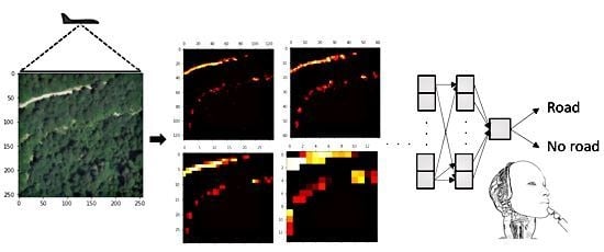
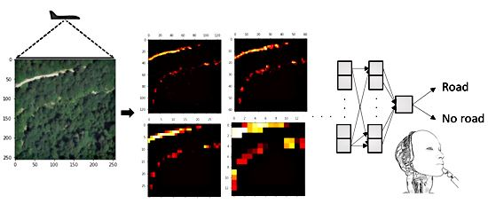
• We design a novel framework based on deep convolutional neural networks to classify secondary roads in high resolution aerial orthoimagery. The solution integrates modified configurations (focusing on improving the computational efficiency) of three of the most popular CNN architectures for computer vision problems, together with a network especially built for this task;
• We contrast the performance of state-of-the-art CNN architectures and deep learning techniques in recognizing secondary roads in high resolution aerial imagery under various scenarios;
• We study how different architectural tweaks and changes in default hyperparameters affect a base model’s performance in the road classification task;
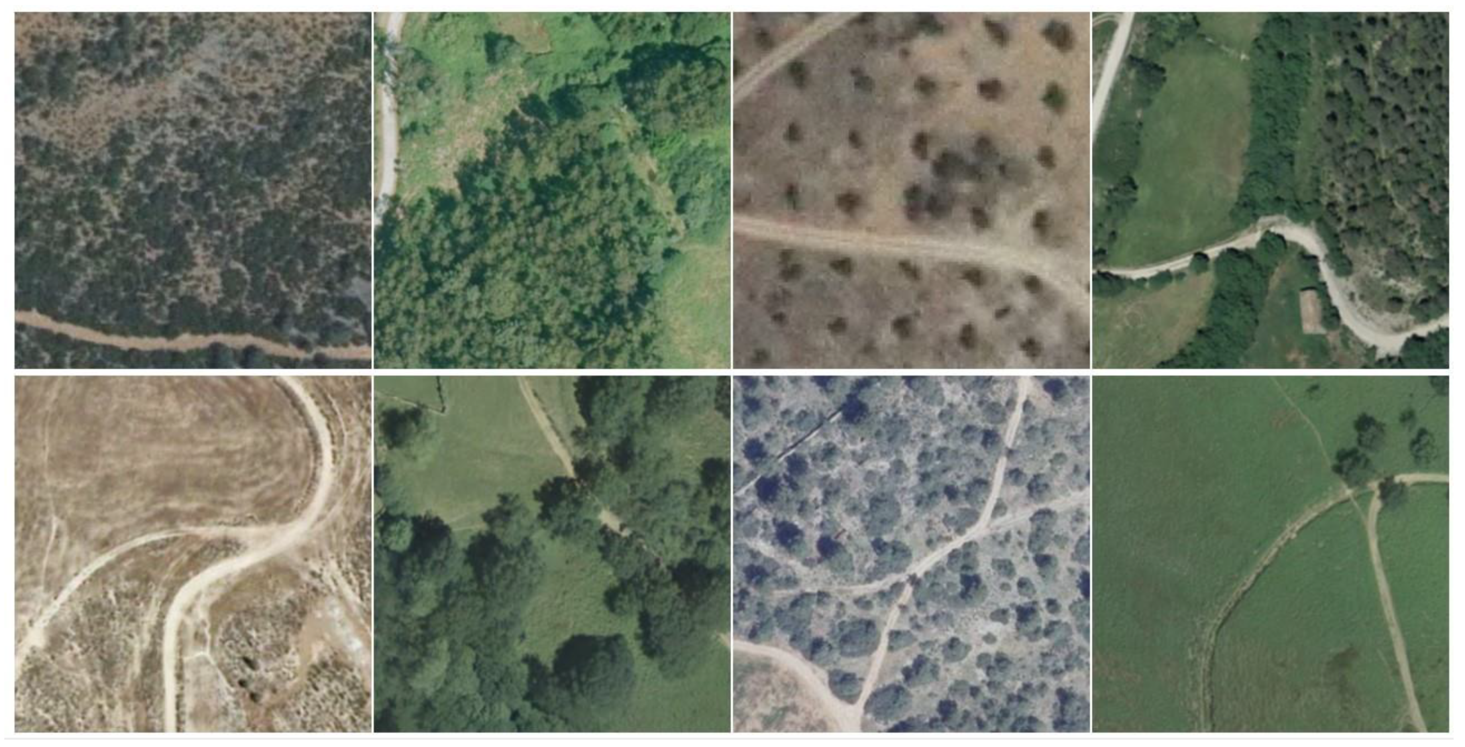
• Different from the previous works, we focus on challenging situations, where the borders of the roads are easily confused with the surroundings (secondary transport routes). In addition, the remotely sensed imagery often includes shadows and occlusions, further complicating the classification operation;
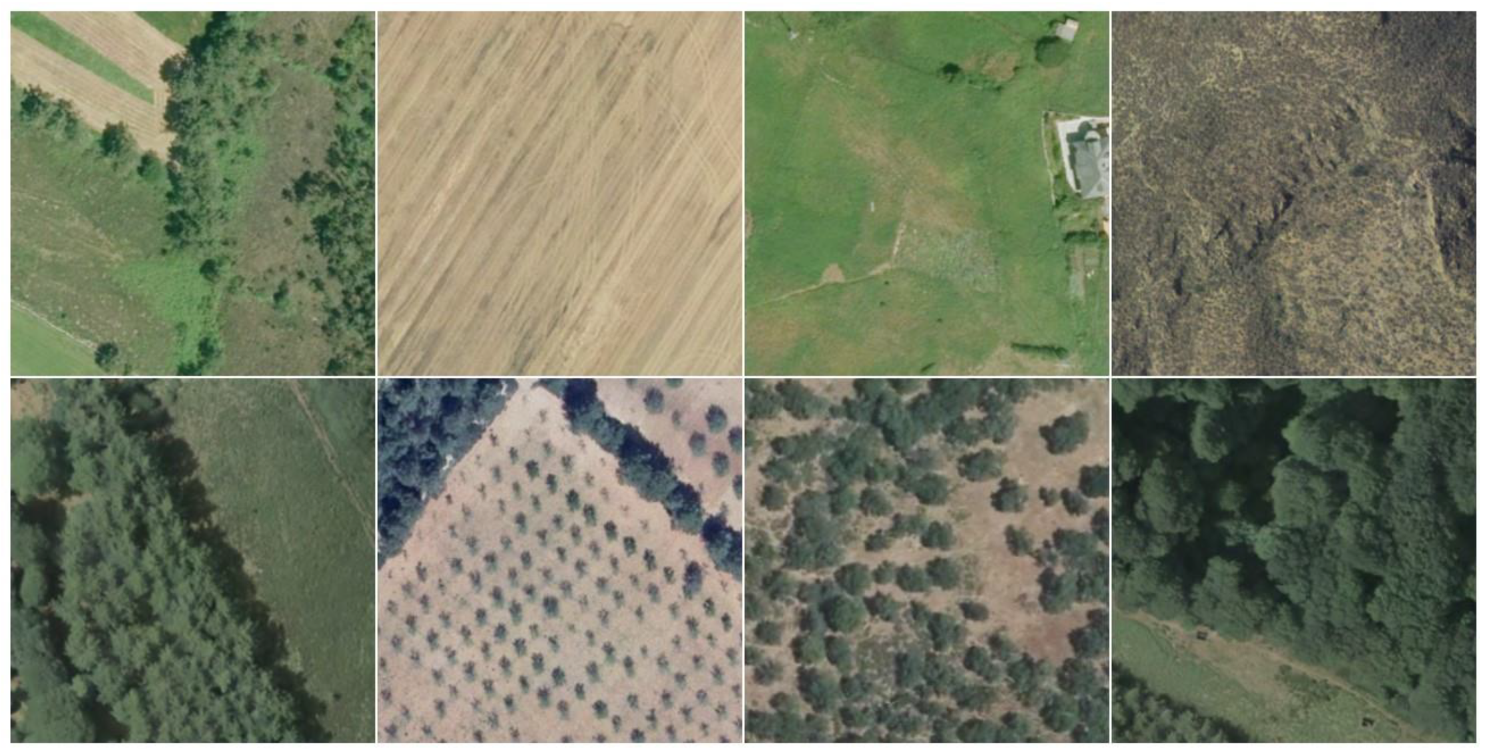
• We carry our experiments on a new dataset composed of sampled locations with ground truth labels obtained by dividing high resolution aerial imagery in tiles of 256 × 256 pixels and manually annotating them.

The remainder of this article is organized as follows. Section 2 describes works related to road detection and classification using remotely sensed data. Section 3 describes the dataset built for this task. Section 4 introduces the architectures used as weak learners and provides details of our proposed framework. Section 5 describes the experiments carried out to obtain the best possible configurations. In Section 6, we present the performance metrics and conduct an extensive discussion and statistical analysis. Lastly, Section 7 draws the conclusions of our work, the last section being reserved for references.

2. Related Work

A wave of promising research was incentivised in the remote sensing community following the success of deep CNN architectures in solving computer vision tasks. These networks are designed to receive images as inputs and encode three important architectural features: (1) shared weights—by forcing the neurons of one layer to share weights, the forward pass becomes the equivalent of convolving a filter over the image to produce a new image (the convolution operation), (2) local connectivity—neurons in one layer are only connected to neurons in the next layer that are spatially close due to a smaller kernel size, and (3) representations—by using pooling and ReLU non-linearities, we increase the model’s expressive power.

It is important to mention that the weights obtained from training popular CNN architectures on ILSVRC (1.2 million images) are publicly available as pre-trained models. We can apply transfer learning to customize these pre-trained models for a new task and take advantage of the learned feature maps. Transfer learning works by initializing the weights of a network using the weights of an already trained model on a large dataset, ensuring a good convergence most of the time [8]. The level of generality of the representation extracted depends on the depth of the layer in the model: earlier layers extract highly generic feature maps (such as edges, colours, textures), whereas layers that are higher up extract more abstract features. Researchers in the field of remote sensing have successfully applied transfer learning to repurpose the pre-learned features for land use analysis and object detection in satellite imagery data.

A hot research area in this field is related to aerospatial objects detection: In [9], the authors constructed a CNN for airport detection, focusing on harder examples by adding a mining layer to automatically detect examples by their losses, obtaining F1-scores of maximum 0.9567 on the validation set. The authors of [10] propose a framework based on deep CNNs to recognize ten types of aircrafts using key-point annotations of the planes in the training stage, obtaining accuracy levels of maximum 95.6%. In [11], the structure of VGGNet was enhanced by replacing the FC layers with a full CNN to improve the performance metrics in airplane and automobile detection, while reducing the number of parameters.

Another important area of research is related to the task of building detection and mapping using remote sensing imagery. In [12], a fine-tuned version of VGGNet is used to detect buildings and recognize the roof types, obtaining quality rates higher than 83.3%. The authors of [13] evaluated the performance of deep learning for roof segmentation on a dataset containing over 220,000 buildings tagged in remote sensing images with a spatial resolution of 7.5 cm and obtained F1-scores of maximum 0.947. In [14], open-source data is used to conduct a comparative analysis between four different CNN architectures pre-trained on large datasets to extract footprints of buildings across the United States, obtaining precision scores higher than 95%.

Other works, such as [15], focused on transferring knowledge from the image scene classification task to the geospatial object detection task using supervision from scene tags to classify nine different categories (including bridges, ships, tennis courts). The authors of [16] implemented a deep CNN comprised by two convolutional and two max-pooling layers followed by two FC layers to predict labels for images captured by UAVs in real time, achieving accuracy levels of 93.6%. In [17], the authors contrast the capabilities of VGG-16 and ResNet architectures in recognizing land use classes and patterns in different urban environments from satellite imagery, obtaining accuracy levels of maximum 81.0%. The authors of [18] investigated the transfer of activations from CNNs pre-trained on ILSVRC to scene classification tasks by extracting activation vectors from the FC layers and by encoding features into global image features to improve the classification accuracies.

Hutchison et al. were among the first to approach the challenge of road detection in urban environments using deep learning. In [19], they used supervised methods to build a model for this task, and later applied unsupervised training to generate filters that improved the predictions of the model.

In [20], a CNN consisting of five convolution layers followed by a GAP layer is proposed to extract roads from publicly available urban road datasets. The inputs were aerial images of 1500 × 1500 pixels in size with a spatial resolution of one meter, and the performance metrics were as high as 81.6%. In the end, they used spatial features of adjacent pixels to enhance multi-class prediction.

The authors of [21] recognized the complexity of road detection in real-world applications while evaluating the performance of the most popular CNN architectures in road detection and segmentation using satellite imagery. They obtained precision levels of a maximum 71.69% by applying data augmentation, filtering and post-processing techniques.

Inspired by residual learning, the authors of [22] developed a deep-residual network similar to U-Net for the semantic segmentation of roads and tested it on a public roads dataset. The performance metrics increased by 1%, while the number of parameters decreased by ¾, when compared to U-Net.

Recently, the authors of [23] proposed RoadNet (composed on three CNN following the VGGNet architecture) to analyse urban scenes and predict road surfaces, edges, and centrelines. The three CNNs were concatenated and used receptive fields of 1 × 1 pixels in size, obtaining F-scores of maximum 93.9%.

In [24], this challenge is approached from a spatio-temporal perspective by adding a temporal processing block on top of existing networks, achieving accuracy levels over 90%. In [25], the authors proposed a model based on VGGNet to learn the features of road boundaries by integrating RGB images street scenes, the semantic contour and the location in a neural network for autonomous driving applications.

3. Dataset

The variables studied in this paper are pixel values of high-resolution aerial orthophotos. The imagery used was issued by state agencies and has a declared spatial resolution of 0.50 m (one pixel covers an area of 50 × 50 cm on the ground) and a planimetric RMSE ≤ 1 m [26].

These data were captured using calibrated high-resolution digital photogrammetric cameras equipped with 3-band RGB sensors (eight bits per band) and is georeferenced in ERTS89 Geodesic Reference System. The photograms were acquired in optimal meteorological conditions (clear sky with no clouds during specific hours and east–west orientation of the flight to minimize the errors caused by the sun). According to its producer, the imagery is orthorectified to ensure matching between contiguous photograms, radiometrically corrected to make effective use of all the bits (homogeneous intensity and balanced histograms) and has topographic corrections applied using terrestrial coordinates of representative points. Considering the low flight altitude, the effect of the atmosphere conditions is considered negligible; therefore, no atmospheric corrections were applied.

The data needed for the supervised learning process were obtained by labelling these orthoimages divided in tiles using a cartographic viewer based on Web Map Service (WMS) [27]. The task involved performing a visual comparison of the most recent orthoimages available with the existing cartographic support. For consistency reasons, we used the same zoom-level during the operation, each tile covering an area of 128 × 128 meters. We took into account representative areas of Spain (Galicia, Navarre, Balearic Islands, Segovia, Ciudad Real, Albacete, Murcia, Huelva) that may influence a network’s capability in identifying secondary roads for the whole national territory. The labelled tiles were merged into the correspondent category (samples extracted from each collection can be seen in Figure 1 and Figure 2). These categories will allow the CNNs to learn about the existence/non-existence of roads in a new given tile.

The dataset created contains 18,000 tiles and occupies a disk volume of approximately 2.62 GB. We are working towards making it openly available once we increase its size. Each image has a height of 256 pixels, a width of 256 pixels (for a total of 65,536 pixels = 0.07 Megapixels) and a depth of three colour channels (RGB). Each pixel in the Red/Green/Blue channel is represented by a number between 0 and 255, where 255 represents the maximum brightness (white) and 0 means no brightness (black).

The difference in performance metrics found in [7] made us build additional subsets with the criteria of similar background colours (areas with dense vegetation/Mediterranean areas) for the second variant of the ensemble model (based on specialized models). We also doubled the size of the dataset used in [6] to expose the models to more aspects of the classes, and balanced the classes to avoid the common machine learning problem where a model starts to predict new observations to the majority class to achieve high accuracy. The tiles’ distribution can be seen in

Table 1. Distribution of the labelled tiles.

Dataset	Category 0 “No Road”			Category 1 “Road Exists”
	Areas with Dense Vegetation	Drier (Mediterranean) Areas	Total	Areas with Dense Vegetation	Drier (Mediterranean) Areas	Total
Total	4500	4500	9000	4500	4500	9000
Percentages	25.00%	25.00%	50.00%	25.00%	25.00%	50.00%

.

4. Framework

Our framework involves model nesting (and more specifically, ensembling) where, given a set of models, we ensemble them using stacking techniques to combine the predictions of the models and build a new model. The reasoning behind using an ensemble is that by stacking multiple models (called base models or weak learners) representing different hypotheses, we can find a better hypothesis that might not be contained within the hypothesis space of the models from which the ensemble is built. In [28], the author identified three main reasons causing this situation: (1) having insufficient input data (statistical), (2) difficulties for the learning algorithm to converge to the global minimum (computational), and (3) representational, where the function $h^{\ast }$ cannot be represented by any of the hypothesis proposed.

A popular form of stacking involves computing the outputs of base models, performing a prediction for each model and averaging their predictions inside the ensemble. In this technique, the sub-models contribute equally to a combined prediction, $\overline{y} \left(x\right)=1/M{\displaystyle \sum }_{m=1}^M{y}_m \left(x\right)$. Firstly, all the algorithms fused into the ensemble are trained using the available data and then a combiner algorithm is used to make a final prediction using the predictions of the other models as inputs. The specific steps are: (1) generate $M$ weak learners, each with its own initial values (by training them separately), and (2) combine these models in an ensemble where we average their predictions for every instance of the dataset to compute $\overline{y}$.

We built the ensemble by combining base models as diversely as possible (Figure 3). We took into consideration the network built in [6], together with modified versions of the most popular CNN architectures for computer vision tasks. This way, we can leverage their strengths and minimize their weaknesses to obtain a classifier with a lower classification error.

Next, we will describe the four base model architectures fused into the ensemble model. Three of these networks are the best performing models on ILSVRC, each based on different architectural patterns (structural blocks and connection schemes). It is important to note that these networks will be modified during the experiments in order to find the best possible configuration for each architecture.

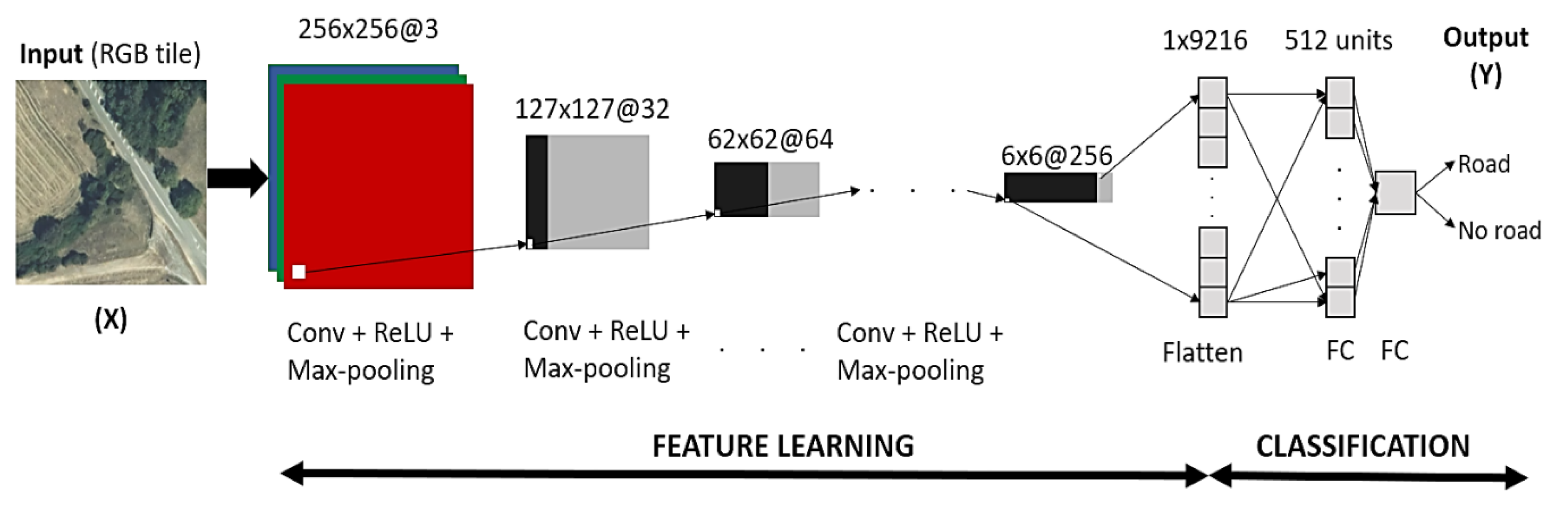
4.1. CNN Built from Scratch

For the first base model, we opted for a CNN formed by a stack of convolutional layers containing filters with a receptive field of 3 × 3 followed by max-pooling layers with 2 × 2-pixel windows. We chose this particular architecture for its simplicity, computational efficiency and flexibility.

In a multilayer convolutional network, the input to the second layer is the output of the first layer, and when we use multiple filters on the same image, we carry out the convolution for each of them separately, piling up the results one on top of the other, and combining them into feature maps. The resulting tensor is finally reshaped to flatten out the spatial dimensions into a one-dimensional feature vector that can be fed into the classifier.

At the end of the network, we have two FC layers: the first contains 512 units, while the second contains one unit (where it performs the 2-class classification). In between these FC layers, we added a dropout layer with a rate of 0.5 to avoid overfitting.

In Figure 4, we can see how a tile is processed through this particular base model.

4.2. VGGNet-Like Network

The second component of the ensemble is a modified version of VGGNet represented by a stack of convolutional blocks formed by two convolutional layers followed by one max-pooling layer. We propose this configuration for its compact architecture. The chosen kernel size is 3 × 3 and the max-pooling step is performed over a 2 × 2-pixel window. After each convolutional block, we added a dropout layer with a rate of 0.25 for a more aggressive control of the overfitting.

The first component of the classifier is a FC layer with 512 neurons connected to a final single unit layer. In between the classifying layers, we added a dropout layer with a rate of 0.5. We also reduced the number of filters/convolution when compared to the standard network. By applying these changes to the original architecture, we drastically reduced the number of parameters from 169 million to a little over 4.5 million. This architecture is described in

Table 2. Description of the modified VGGNet architecture.

Block1	Block2	Block3	Block4	Block5	Output Block
Conv (3 × 3, 32)	Conv (3 × 3, 64)	Conv (3 × 3, 64)	Conv (3 × 3, 64)	Conv (3 × 3, 128)	Flatten
Conv (3 × 3, 32)	Conv (3 × 3, 64)	Conv (3 × 3, 64)	Conv (3 × 3, 64)	Conv (3 × 3, 128)	FC (512)
Maxpool (2 × 2)	Maxpool (2 × 2)	Maxpool (2 × 2)	Maxpool (2 × 2)	Maxpool (2 × 2)	Dropout (0.5)
Dropout (0.25)	Dropout (0.25)	Dropout (0.25)	Dropout (0.25)	Dropout (0.25)	FC (1, sigmoid)

.

4.3. Modified ResNet

The Residual blocks (introduced by He et al. in [4]) allow for the training of very deep networks by introducing modules called residual models. These blocks address the degradation problem observed when training deep neural networks by allowing the gradient to flow through the alternate shortcut path, ensuring the movement of information from earlier layers in the model to latter layers.

Our implementation consists of a modified version of ResNet50, where we stack Convolutional and Identity blocks on the residual connections (that allow the flow of information while enabling the learning of an identity function). Compared to the original ResNet50, we reduced the number of filters/convolutions and changed the activation functions from ReLU [29] to PReLU [30] and LeakyReLU [31]. Our top block includes a GAP layer with a 2 × 2-pi×el window (replacing the window area with the average value instead of the maximum value) followed by a Flatten layer and a FC layer with a softmax activation (where the classification is performed). By applying these changes, the number of total parameters dropped from 25.6 million to 5.9 million, resulting in a more efficient computation.

Details about the modified VGG50 network can be seen in

Table 3. Description of the modified ResNet-50 Architecture.

Stage	Structure	Output Size (Volume)
1	Conv (7 × 7, 32, stride = 1) + BN + Activation Maxpool (3 × 3)	Input = 256 × 256 × 3 Output= 85 × 85 × 32
2	ConvBlock (3 × 3, [32,32,64], stride = 1) 2 × (ID_block (3 × 3, [32,32,64])	85 × 85 × 128
3	ConvBlock (3 × 3, [64,64,256], stride = 2) 3 × (ID_block (3 × 3, [64,64,256])	43 × 43 × 256
4	ConvBlock (3 × 3, [128, 128, 256], stride = 2) 4 × (ID_block (3 × 3, [128, 128, 256])	22 × 22 × 512
5	ConvBlock (3 × 3, [256, 256, 1024], stride = 2) 2 × (ID_block (3 × 3, [256, 256, 1024])	11 × 11 × 1024
Output	Global Average Pooling (2 × 2) FlattenFC ($n$ classes, softmax)	5 × 5 × 1024 15,600 2
ConvBlock: Conv (1 × 1, [Filter], stride = 1) + BN + Activation          BN = Batch Normalization Conv (KernelSize, [Filter], stride = 1) + BN + Activation Conv (1 × 1, [Filter]) + BN Shortcut = Conv (1 × 1, [Filter], stride = s) + BN Add (Shortcut + ID_block) + Activation
ID_block: Conv (1 × 1, [Filter], stride = 1) + BN + Act, stride = s Conv (KernelSize, [Filter], stride = 1) + BN + Act Conv (1 × 1, [Filter], stride = 1) + BN Add (ID_block + Shortcut) + Act

.

4.4. Inception-ResNet

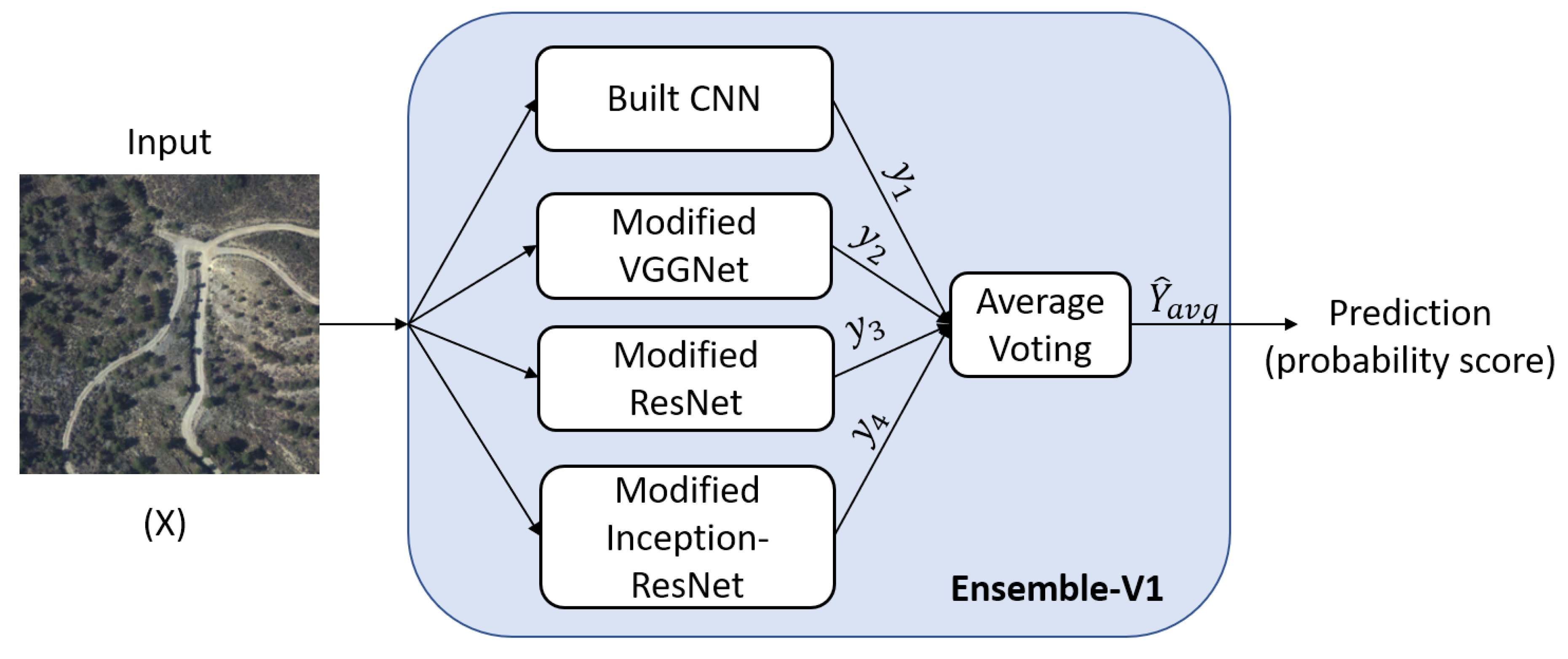
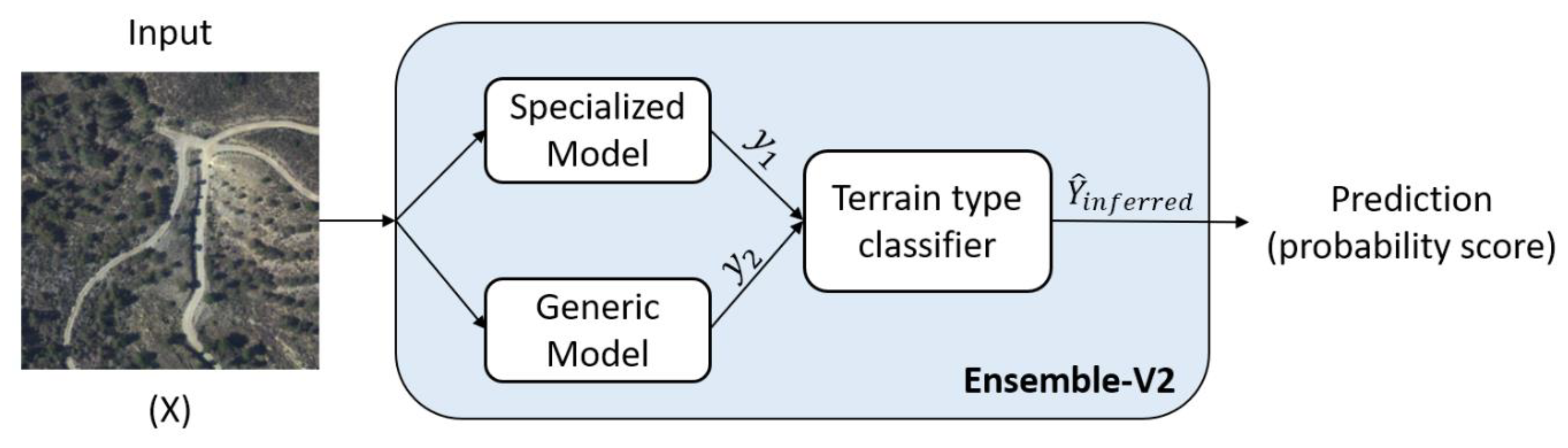
In 2015, Inception-v2 and Inception-v3 [32] proposed a number of upgrades over the original Inception architecture to increase the accuracy and reduce the computational complexity: Inception-v2 introduced factorization (factorizing convolutions into smaller convolutions: traditional 7 × 7 convolution into three 3 × 3 convolutions), while Inception V3 added Batch Normalization-auxiliary (in which the FC layer is also-normalized, not just the convolutions; batch normalization reduces the amount by what the hidden unit values shift around and allows each layer of a network to learn by itself with a higher degree of independency).

Inception-ResNet [5] was introduced the following year, together with the fourth iteration of Inception (v4). Here, the authors focused on making the modules more uniform and simplifying some of them, while adding Residual blocks to enable the gradient flow through shortcuts added to main path. This architecture obtained the highest score at ILSVRC 2016.

Given the increased complexity of this architecture, we only modified the classifier added on top of the convolutional base and applied transfer learning techniques while tweaking the standard hyperparameters. The classifier added on top consists of a GAP layer over a 2 × 2-pixel window, a FC layer with 512 neurons using ReLU activation function, a Dropout layer with a rate of 0.5 and a final FC layer of size 1 using sigmoid activation function.

4.5. Ensemble-V2

On the other hand, as stated in the introduction, we wanted to address the significant difference in performance found in [7] when testing the models on data with different vegetation coverage separately. We propose a second variant of the ensemble model (Figure 5) using a specialized model on the subset only formed by tiles from the area with the lower performance metrics and a generic model trained on the entire dataset. Their predictions will be fed into a terrain type classifier (which will act as an arbitrary combiner algorithm) that infers the type of vegetation the tile contains and decides which of the two predictions will be the final one. In other words, the ensemble will use a network to infer the type of vegetation coverage in a tile and, based on that result, will decide the final prediction.

5. Experiments

The goal is to learn a classifier that can input an image represented by a feature vector (tensor) X and predict whether the corresponding label is 1 or 0. The learning process is done using convolution operations, which preserve the relationship between pixels by learning image features (moving from discriminating features at a local level in the earlier layers towards generalizing these features at a global level in the later layers). Convolution ($\ast$) is an operation on two functions $S\left[i,j\right]=\left(K\ast I\right)\left( i, j\right)={\displaystyle \sum }_m{\displaystyle \sum }_{n}I\left(i-m, j-n\right)K\left(m,n\right),$ where the first argument is referred to as the input (the function I is a 2-D array with two indices ($m,n$) of the spatial coordinates of pixels), the second argument is referred as the kernel, while the output $S$ is referred as a feature map. We can say that $S$ is produced by convolving filter $K$ of dimensions $m,n$ across all the input $I$ of dimensions $i,j$. In the case of RGB images, we have to add one more index of the different colour channels (resulting a 3-D tensor); software implementations usually work in batch mode, so we have to add a fourth axis indexing the samples in the batch (4-D tensors) [33].

In our case, a single training example is represented by a pair $\left(x,y\right)$, where $x$ is an 3-D feature vector and $y$ (the label) is either 0 or 1. Our dataset (Table 1) comprises of $n=\mathrm{18,000}$ samples $\left(x^{\left(1\right)}, y^{\left(1\right)}\right), \dots , \left(x^{\left(n\right)}, y^{\left(n\right)}\right)$ with dimensions of 256 × 256 × 3. We split our dataset by randomly assigning the tiles into the following three sets:

• A full training set of 14,400 tiles (80% of the data) and five training subsets containing 90% of the full training set (12,960 tiles) with their corresponding labels were used to perform the weights initialization. The five subsets represent variations of the training population and were used to repeat the experiments and to conduct a statistical analysis of the performance metrics;
• A validation set (10% of the data) was formed by 1800 tiles and used for tuning the model’s hyperparameters and comparing how changing them would affect the model’s predictive performance;
• A test set (10% of the data) containing 1800 tiles to evaluate the performance of the models on unseen data.

According to the literature conventions [34,35], we have also considered other data splits, but the initial results were lower (as seen in

Table 4. Results of the initial tests.

Data Split	Metric	Initial Results (Each Column Represents a Trained Configuration)
50%-25%-25%	Loss	0.2219	0.2411	0.2123	0.2233	0.1601	0.1816
	Accuracy	0.9262	0.9271	0.9264	0.9331	0.9409	0.9391
	Precision	0.8829	0.9158	0.8693	0.8379	0.8554	0.8686
	Recall	0.8916	0.8604	0.9107	0.8613	0.8569	0.8431
	F1 score	0.8800	0.8873	0.8895	0.8494	0.8561	0.8557
60%-20%-20%	Loss	0.2139	0.2087	0.1729	0.1901	0.1696	0.1678
	Accuracy	0.9372	0.9355	0.9433	0.9361	0.9406	0.9394
	Precision	0.9028	0.8978	0.9137	0.9099	0.9137	0.9096
	Recall	0.8978	0.9078	0.9056	0.8867	0.8944	0.8944
	F1 score	0.9003	0.9028	0.9096	0.8981	0.9040	0.902
80%-10%-10%	Loss	0.1560	0.1811	0.1624	0.1468	0.1733	0.1551
	Accuracy	0.9511	0.9461	0.9483	0.9533	0.9367	0.9472
	Precision	0.9133	0.9068	0.9198	0.9216	0.8938	0.9244
	Recall	0.9133	0.9078	0.9044	0.9011	0.8978	0.8967
	F1 score	0.9133	0.9073	0.912	0.9112	0.8958	0.9103

) when compared to the 80%-10%-10% split described above, so we decided to carry on the experiments only with the data split allowing for more training data. The other mentioned splits favour higher ratios of validation and testing data and could be the preferable approach when dealing with very large datasets, but are not desired when tackling complex classification tasks with limited datasets.

We implemented the framework and the base models presented in Section 4 in the open-source Python deep learning library Keras [36] (with TensorFlow 1.14 [37] as backend) using an NVIDIA 2060 GPU mounted on a system with a 12-core Intel I7-8700 CPU and 16 GB RAM.

In all the experiments, we applied data augmentation techniques on the training set, including random horizontal and vertical flipping of the input images, random rotations, random horizontal and vertical translations and random zooms to avoid overfitting and allow the model to generalize better, given that it never sees the same tile twice. To avoid losing important information around the edges of the tile, we used small augmentation parameters. To fill out the pixels created after these operations outside the boundaries of the input, we used the ‘nearest neighbour’ interpolation technique. An example of data augmentation applied to a random tile can be seen in Figure 6. It is important to note that the batches of augmented tensor image data used for training were generated in-memory in real-time and were not stored on the disk.

In the experiments, we used stochastic gradient descent to optimize the network’s loss (cost) function (a standard binary-class cross-entropy). As activation functions, we generally used ReLU non-linearity for the convolutional layers and the first FC layer and sigmoid for the last FC layer (encoding the probability of a class or the other).

For training, we used small learning rates (from $1\times e^{-6}$ up to $1\times e^{-2}$) to ensure a stable learning process and chose a standard number of 100 epochs for an initial observation of the network’s behaviour (this number was subsequently increased or decreased depending on the network’s convergence). The goal of the experiments was to identify the classifiers with the lowest classification error for each of the architectures proposed.

In the case of the CNN formed by stacked convolutional layers followed by max-pooling layers (presented in Section 4.1), we modified the number of filters/convolutions, the network’s depth (to obtain feature maps of different sizes), and we increased the size of the kernel from 3 × 3 to 5 × 5. The optimizer used in all scenarios was Adam [38] (considered to be the fastest to converge [39]) with a learning rate of $1\times e^{-4}$.

In the case of the VGGNet-like architecture (proposed in 4.2), we gradually increased the number of convolutional blocks from three to five and applied a different number of filters/convolution blocks (from [32, 64, 64] to [32, 64, 64, 64, 128]). We also used different optimizers to study their impact on the learning process: Adam with learning rates (lr) of $1\times e^{-3}$/$1\times e^{-4}$, the standard SDG [40] (with a learning rate of $1\times e^{-2}$, decay of $1\times e^{-5}$ and Nesterov Momentum [41] of $9\times e^{-1}$ as proposed by the authors of [3]) and an RMS props optimizer [42] with a learning rate of $1\times e^{-4}$. The classifier was also modified by choosing different number of units in the first FC layer (256 and 512) and by using a GAP layer instead of Flatten before the FC layers [43].

Furthermore, we also applied transfer learning techniques (especially fine-tuning, where we unfreeze a portion of the layers from a frozen convolutional base and retrain them together with the classifier added on top). In [7], we observed that pre-trained models are sensible to changes, their performance changing depending on where we start to update the weights—retraining starting from a network´s early levels lowered the performance (updating the weights damaged the features learnt [44]); therefore, we only fine-tuned the upper convolutional blocks.

In the case of ResNet, we trained the architecture proposed in Chapter 4.3 after modifying the number of layers/convolution and using different activation functions (ReLU, PReLU and LeakyReLU). Given the complex nature of Inception-ResNet, we only applied transfer learning techniques: feature extraction (retraining the classifier added on top) and fine-tuning for the last convolutional blocks with learning rates of $1\times e^{-3}$ and $1\times e^{-6}$. Finally, we trained the original networks from scratch for comparison. The training scenarios described above are presented in

Table 5. Training scenarios.

Nº	Base Architecture		Configuration	Filters/Conv (Block)	Size of the Last Feature Map	FC Units (Classifier)	Optimizer and Learning Rate	Other Aspects
1	Built CNN (Figure 1)		4 × convolutional blocks	[32, 64, 128, 128]	14 × 14 × 128	512, 1	Adam (lr = $1\times e^{-4}$)	-
2			5 × convolutional blocks	[32, 64, 128, 128, 128]	6 × 6 × 128
3			5 × convolutional blocks	[32, 64, 128, 128, 256]	6 × 6 × 256
4			5 × convolutional blocks	[32, 64, 128, 256, 512]	6 × 6 × 512
5			5 × convolutional blocks	[32, 64, 128, 128, 256]	4 × 4 × 256			Filter size = 5 × 5
6	VGGNet	VGG–like CNN (Table 2)	3 × convolutional blocks	[32, 64, 64]	28 × 28 × 64	256, 1	SDG (lr = $1\times e^{-2}$, decay = $1\times e^{-5}$, Nesterov momentum = $9\times e^{-1}$)	-
7			4 × convolutional blocks	[32, 64, 64, 64]	12 × 12 × 64	512, 1
8			5 × convolutional blocks	[32, 64, 64, 64, 128]	8 × 8 × 128	512, 1
9			5 × convolutional blocks	[32, 64, 64, 64, 128]	8 × 8 × 128	512, 1	Adam (lr = $1\times e^{-4}$)
10			5 × convolutional blocks	[32, 64, 64, 64, 128]	8 × 8 × 128	256, 1
11		Standard [3]	Fine-tuning the last convolutional block (ImageNet weights)	Default configuration [3]	8 × 8 × 512	512, 1	Adam (lr = $1\times e^{-3}$)	Global Average Pooling instead of Flatten
12							Adam (lr = $1\times e^{-4}$)
13							RMSprop (lr = $1\times e^{-4}$)
14			No weights (from scratch)			[3]	Adam (lr = $1\times e^{-4}$)	MSRA [30] initialization
15	Resnet50		Modified ResNet	Described in Table 3			Adam (lr = $1\times e^{-4}$)	Activation = ReLU
16								Activation = Leaky ReLU
17								Activation = PReLU
18			No weights (from scratch)	Default configuration [4]	8 × 8 × 2048	[4]	Adam (lr = $1\times e^{-4}$)	-
19	Inception-ResNet		Feature Extraction	Default configuration [5]	6 × 6 × 1536	512, 1	Adam (lr = $1\times e^{-4}$)	Global Average Pooling instead of Flatten
20			Fine-tuning the last module				Adam (lr = $1\times e^{-6}$)
21			Fine-tuning the last 2 modules				Adam (lr = $1\times e^{-3}$)
22			No weights (from scratch)			[5]	Adam (lr =$1\times e^{-4}$)	-
23	Ensemble		Variant I: Average Voting	Described in Figure 3				-
24			Variant II: Specialized model	Described in Figure 5

.

6. Results and Discussion

After selecting the weights using the training and validation sets, we evaluated the generalization capacity of the models using the test set containing unseen data (with a support of 900 tiles for each class) and obtained the confusion matrices (or error matrices) of the classification operation (an example can be found in Figure 7).

From the confusion matrices, we calculated the following performance metrics: precision (the number of true positive predictions divided by the total number of positive class values), recall (the number of true positive predictions divided by the number of true positives and false negatives) and F1 score (indicating the balance between the precision and the recall). The last metric is the Area Under the Receiver Operating Characteristic Curve (ROC–AUC) computed from prediction scores. This measure tends towards 1.0 when only a little precision has to be sacrificed to get a high recall, and towards 0.5 for the opposite case, and shows how much a model is capable of distinguishing between classes.

To statistically analyse the results, we repeated the training and evaluation of the configurations described in Table 5 using the five training subsets (containing 12,960 tiles randomly obtained from the full training set).

After an initial evaluation of the proposed configurations, we selected the best performing ones and stacked them as described in Figure 3 and Figure 5. This way, the first variant of ensemble model averages their predictions of the models resulting from training scenarios 2, 11, 15 and 20. For the second variant of the ensemble, we selected three weak learners: a generic model (configuration 4, trained on the whole dataset) and a specialized model (based on configuration 11 retrained on a dataset containing only tiles from the Mediterranean areas, where it obtained a AUC–ROC score of 0.9697), together with a terrain type classifier trained to infer the ensemble’s prediction based on the vegetation coverage in a tile (based on configuration 2, which obtained an accuracy score of 0.9628, with a loss of 0.0989 on the validation set). Here, given the prediction of the specialized model in classifying roads in Mediterranean areas and the prediction of a generic mode, we are left with the one inferred by the classifier trained to detect the type of vegetation coverage in a tile (the generic prediction if the classifier detects green areas or the prediction of specialized weak learner in the opposite case).

The performances of the configurations were afterwards compared using one-way analysis of variance (ANOVA) with the performance metric as the dependent variable and the configurations as the levels of a fixed factor. To test the null hypothesis that the performances of all configurations are the same, the $F$ statistic is computed from the ANOVA table and reported in

Table 6. Mean (M) and standard deviation (SD) of the performance metrics obtained by the configurations described in Table 5.

Config. Nº	Accuracy		Loss		Precision		Recall		F1		AUC–ROC
	M	SD	M	SD	M	SD	M	SD	M	SD	M	SD
1	0.931	0.003	0.183	0.005	0.907	0.017	0.891	0.026	0.899	0.006	0.949	0.002
2	0.940	0.006	0.164	0.014	0.912	0.010	0.897	0.007	0.922	0.035	0.952	0.003
3	0.938	0.004	0.166	0.012	0.913	0.010	0.892	0.016	0.902	0.005	0.950	0.003
4	0.940	0.007	0.170	0.012	0.913	0.008	0.892	0.021	0.902	0.008	0.950	0.003
5	0.936	0.005	0.184	0.005	0.903	0.011	0.894	0.007	0.898	0.005	0.943	0.001
6	0.941	0.005	0.178	0.022	0.903	0.005	0.905	0.008	0.904	0.004	0.948	0.004
7	0.945	0.002	0.162	0.010	0.914	0.004	0.899	0.003	0.906	0.002	0.948	0.003
8	0.943	0.007	0.164	0.019	0.893	0.047	0.898	0.012	0.906	0.006	0.948	0.003
9	0.943	0.003	0.157	0.006	0.914	0.009	0.896	0.006	0.905	0.002	0.949	0.003
10	0.943	0.002	0.157	0.002	0.909	0.009	0.903	0.007	0.906	0.002	0.948	0.002
11	0.945	0.002	0.169	0.013	0.919	0.012	0.917	0.014	0.918	0.013	0.967	0.002
12	0.945	0.004	0.190	0.017	0.912	0.007	0.909	0.008	0.911	0.008	0.964	0.002
13	0.928	0.026	0.281	0.034	0.939	0.018	0.941	0.021	0.940	0.019	0.956	0.009
14	0.939	0.008	0.157	0.015	0.916	0.017	0.913	0.020	0.914	0.018	0.967	0.001
15	0.923	0.008	0.201	0.026	0.919	0.006	0.917	0.007	0.921	0.006	0.952	0.003
16	0.920	0.029	0.189	0.027	0.920	0.018	0.918	0.020	0.922	0.018	0.946	0.006
17	0.917	0.014	0.219	0.035	0.922	0.009	0.922	0.011	0.924	0.009	0.948	0.003
18	0.910	0.012	0.218	0.022	0.929	0.020	0.934	0.024	0.932	0.022	0.956	0.003
19	0.863	0.011	0.403	0.031	0.946	0.006	0.958	0.006	0.952	0.006	0.931	0.002
20	0.862	0.003	0.326	0.011	0.954	0.003	0.965	0.003	0.960	0.003	0.938	0.003
21	0.875	0.032	0.389	0.111	0.953	0.009	0.962	0.011	0.958	0.010	0.930	0.021
22	0.934	0.013	0.172	0.031	0.939	0.002	0.942	0.002	0.941	0.002	0.962	0.004
23	0.956	0.002	0.132	0.008	0.966	0.006	0.945	0.005	0.955	0.002	0.991	0.001
24	0.946	0.003	0.156	0.014	0.953	0.012	0.938	0.018	0.946	0.004	0.984	0.002
Total	0.928	0.028	0.204	0.076	0.924	0.023	0.919	0.027	0.923	0.023	0.953	0.015
F-statistic	22.738		29.680		8.768		15.042		14.423		34.520
p-value 1	0.000		0.000		0.000		0.000		0.000		0.000

¹ A p-value smaller than 0.05 implies that null hypothesis is to be rejected at a level of significance of 5% and there is a significant difference in performance between the configurations.

for each of the performance metrics. The alternative hypothesis is that at least one of the configurations has a different performance than the others.

In Table 6, we observe that all p-values are smaller than 0.001; therefore, the configurations are significantly different in each of the performance metrics. However, the analysis of variance $F$-statistics and their p-values does not reveal which configurations are different from the others when there is a significant difference. To have a detailed comparison of the performance of the configurations in different metrics, Figure 8 shows the boxplots of the performances for different configurations.

Figure 8 shows that the two versions of the ensemble (configurations 23 and 24) obtained the highest overall accuracies, precisions and AUC–ROC scores, while obtaining the lowest losses. The lowest accuracies, ROC–AUC scores and the maximum losses are observed when applying transfer learning (feature extraction and fine-tuning) to Inception-ResNet (configuration 19, and 20 and 21). Among Inception-ResNet base architecture, configuration 22 (where we trained the network from scratch) obtained a significantly higher accuracy compared to configurations 19, 20 and 21. The maximum average recall and F1 score is observed for configuration 20, closely followed by 21, while the lowest recall and F1 score is observed for configuration 1.

The accuracies obtained by configurations 1 – 14 are similar, with small variations in the 93.1–94.5% interval. The lowest precision was obtained by configuration 6, while the precisions for configurations 1–12, 14–17 are very similar. Except for configurations 11–14 and 22, all other configurations have very similar AUC–ROC values (between 0.935–0.945).

Configuration 13 has a significantly higher recall and F1-score compared to the other VGGNet architecture configurations. We can see that by fine-tuning VGGNet’s pre-trained weights, we obtained the highest single results. One reason for this might be the VGGNet’s compact architecture, designed to gradually increase the semantic complexity. It is important to note that VGG16 trained from scratch (configuration 16) only converged when applying He normal (MSRA) initializer [35] to the first FC layer.

Next, to formally analyse the pairwise comparison of performances of the configurations in terms of AUC-ROC (the metric score preferred and considered one of the most appropriate for image classification tasks in [45]), we present the post-hoc test results for AUC-ROC using Tukey’s HSD test. Tukey’s HSD test statistic compares two configurations at a time using a $t$-test adjusted for overall variability of the data. The post-hoc tests are designed in such a way that it maintains the level of significance or the probability of type I error at 5% with all pairwise comparisons taken together.

Table 7. Homogenous subset of configurations with post-hoc tests for area under curve (AUC)–receiver operating characteristic (ROC).

Config. Nº	Homogeneous Subsets
	1	2	3	4	5	6	7	8
21	0.930
19	0.931
20	0.938	0.938
5	0.943	0.943	0.943
16		0.946	0.946	0.946
10		0.948	0.948	0.948
8		0.948	0.948	0.948
6		0.948	0.948	0.948
7		0.948	0.948	0.948
17		0.948	0.948	0.948
9		0.949	0.949	0.949
1		0.949	0.949	0.949
3		0.950	0.950	0.950	0.950
4		0.950	0.950	0.950	0.950
2			0.952	0.952	0.952	0.952
15			0.952	0.952	0.952	0.952
13				0.956	0.956	0.956	0.956
18				0.956	0.956	0.956	0.956
22					0.962	0.962	0.962
12						0.964	0.964
14							0.967
11							0.967
24								0.984
23								0.991
Sig.	0.057	0.051	0.436	0.395	0.077	0.061	0.179	0.907

reports the homogenous subsets of configurations in terms of AUC–ROC score.

Configurations within a homogenous subset are not significantly different from each other at a 5% level of significance. For example, configurations 21, 19, 20 and 5 do not have significantly different AUC–ROC scores. However, configurations that are not common in two homogenous subsets are significantly different. For example, configurations 23 and 24 (the ensemble variants) are not significantly different from each other but have significantly higher AUC–ROC compared to all other configurations. These post-hoc test results asserts our observations in Figure 8 boxplots.

On the other hand, by plotting the training time, the number of parameters and the number of epochs before convergence (Figure 9) and crossing the data with data from Table 5, we can study the effect of the hyperparameters on the training behaviour.

We can observe that the training time was highly dependent on the number of trainable parameters, which in turn is dependent on the depth of the networks, the number filters applied in each layer, and the number of units in the classifier.

Changing the activation functions (configurations 15–17) increased the number of parameters from 6 to 17 million, while not significantly improving the results. A higher number of convolutional blocks and a higher number of units in the classifier allowed the networks to better learn the characteristics of the secondary roads with the downside of higher computational needs. Increasing the size of the filters (from 3 × 3 to 5 × 5—configuration 5) did not improve the results and resulted in a more pronounced overfitting behaviour. Using the Adam optimizer resulted in a convergence twice as fast when compared to SDG (configurations 6–9) and 1.5 times faster when compared to RMSprop [46] (configuration 13).

Next, we compared the performances of the configuration grouped on their base architectures using one-way analysis of variance (ANOVA) with the performance metric as the dependent variable and the base architecture as the levels of a fixed factor.

To test the null hypothesis that the performances of all architectures are the same, the $F$-statistic is computed from the ANOVA table and reported in

Table 8. Mean (M) and standard deviation (SD) of the performance metrics obtained by the configurations described in Table 5 grouped by their base architectures.

Base Architecture	Accuracy		Loss		Precision		Recall		F1		AUC–ROC
	M	SD	M	SD	M	SD	M	SD	M	SD	M	SD
Built CNN	0.937	0.006	0.174	0.013	0.910	0.011	0.893	0.016	0.905	0.018	0.949	0.004
VGG-like CNN	0.943	0.004	0.164	0.015	0.907	0.022	0.900	0.008	0.905	0.003	0.948	0.003
VGGNet	0.939	0.014	0.199	0.054	0.921	0.017	0.920	0.020	0.921	0.018	0.964	0.006
Resnet50	0.917	0.017	0.207	0.028	0.923	0.014	0.923	0.017	0.925	0.015	0.951	0.005
Inception-ResNet	0.883	0.035	0.322	0.109	0.948	0.008	0.957	0.011	0.953	0.010	0.940	0.016
Ensemble-V1	0.956	0.002	0.132	0.008	0.966	0.006	0.945	0.005	0.955	0.002	0.991	0.001
Ensemble-V2	0.946	0.003	0.156	0.014	0.953	0.012	0.938	0.018	0.946	0.004	0.984	0.002
Total	0.928	0.028	0.204	0.076	0.924	0.023	0.919	0.027	0.923	0.023	0.953	0.015
F-statistic	32.480		23.600		27.736		46.689		39.445		49.889
p-value 1	0.000		0.000		0.000		0.000		0.000		0.000

¹ A p-value smaller than 0.05 implies that null hypothesis is to be rejected at a level of significance of 5% and there is a significant difference in performance between the configurations.

for each of the performance metric. The alternative hypothesis is that at least one of the architectures has a different performance than the others. We can observe that all p-values are smaller than 0.001; therefore, the base architectures are significantly different in each of the performance metrics. However, the analysis of variance with $F$-statistics and their p-values do not reveal which architectures are different from the others when there is a significant difference. To have a detailed comparison of the performance of the architectures in different metric, Figure 10 shows the boxplots of the performances for the base architectures.

To formally analyse the pairwise comparison of performances of the architectures in terms of AUC–ROC scores, we present the post-hoc test results using Tukey’s HSD test in

Table 9. Homogenous subset of configurations with post-hoc tests for AUC–ROC.

Base Architecture	Homogenous Subset
	1	2	3	4
Inception-ResNet	0.940
VGG-like CNN	0.948	0.948
Built CNN	0.949	0.949
Resnet50		0.951
VGGNet			0.964
Ensemble-V2				0.984
Ensemble-V1				0.991
Sig.	0.158	0.988	1.000	0.346

. Tukey’s HSD test statistic compares two architectures at a time using a $t$-test adjusted for the overall variability of the data. Architectures within a homogenous subset are not significantly different from each other at 5% level of significance.

We can see again that the ensemble architectures do not have significantly different AUC–ROC scores among themselves, but they have significantly higher AUC–ROC scores compared to all other architectures. They are followed by VGGNet, which has a significantly higher AUC–ROC score than ResNet50, Built CNN, VGG-liked CNN and Inception-ResNet, but significantly lower AUC–ROC score compared to Ensemble V1 and V2. VGG-like CNN, CNN and ResNet50 architectures are not significantly different in AUC–ROC among themselves but ResNet50 has a significantly higher AUC–ROC than Inception-ResNet. These post-hoc test results asserts our observations in Figure 10 boxplots.

We can observe significant improvements; the two variants of the ensemble obtain considerably lower error rates when compared to the weak learners evaluated separately. The classifier with the lowest classification errors (Ensemble-V1, based on average voting between four models) obtained an increase in performance metrics by the order of 3–4%. These values are remarkable considering the computational optimization of the weak learners stacked (Figure 10).

Ensemble-V2 (Figure 5) used a weak learner to detect the vegetation coverage in a tile and, based on that probability, it decided on the use of the prediction provided by the generic base model or the prediction of the base model specialized in classifying roads in Mediterranean areas. This architecture obtained improvements of 2–3% when compared to the single generic model (configuration 11). We believe this value can be further improved by increasing the size of the subset used for training the base model specialized in detecting roads in areas with Mediterranean vegetation coverage (the current 3600 tiles/category can be considered insufficient). These models were exported to hdf5 format and can be later deployed in production.

By constructing an ensemble, the learning algorithms were able to learn about the complexity of the road characteristics by leveraging the weaknesses of each architecture to find a better hypothesis and improve the performance metrics. On the other hand, even though we reduce the risk of choosing the wrong classifier, we noticed a lack of sufficient data, especially when trying to build a specialized model. We consider that, in order to progress correctly in the design and evaluation of CNN architectures, it is essential to have a larger data set taking into account the complexity of the road detection task (geometry, soil types, difference in size).

Regarding the transfer learning operation, we found that by initializing the network from pre-trained weights, the performance metrics were greatly improved (by the order of 8–10%) when compared to random initialization. This enabled a better convergence, even though our task was very different from the original one, and proved the effectiveness of the operation. When using transfer learning it is important to apply stronger regularization to control the overfitting behaviour, which occurs when the model has too many degrees of freedom and starts overcomplicating the true structure of the data [47], resulting in models unable to perform well on testing data.

We have mentioned earlier that the characteristics learned by CNN are a representation of real visual concepts. We can visualize the activations produced by performing several convolutions to understand how the input image was decomposed into the features the network learned. For example, in Figure 11, we can visualize activations produced by one of the configurations and see how it “learned” that a road is probably a straight, continuous line. After running a linear activation through a nonlinear activation function (detector stage, e.g., ReLU), we use a pooling function to modify the output of the layer further and reduce its dimensions. We can see that the networks trained for road classification are able to detect even secondary roads that are almost indistinguishable by humans. In the image below, we can see that the model correctly identified the main road and started to mark a potential second road, that is much more difficult to perceive.

7. Conclusions and Future Lines of Research

Ensembling multiple models proved to be a powerful technique to boost the performance of our deep learning system for continuous objects detection in aerial images. We saw that by nesting two or more weak learners (modified versions of popular CNN architectures), our framework built for the road classification task obtained an increase of 2–3% in performance (achieving AUC–ROC scores superior to 0.99) when compared to the base architectures. The results prove the effectiveness of model nesting techniques; at the end of the training process, the proposed framework achieved significantly better generalization scores on unseen data. These high performance scores (the first variant of the ensemble reached accuracy levels of 0.9661 when trained on the full dataset) can also be considered an indicator of the appropriateness of approaching the road extraction task with a classification subtask.

The generalization scores show a low level of overfitting and prove that the characteristics needed for recognizing the labels were included in the training dataset. However, we consider that a production model used to detect roads will require a bigger initial dataset with much more variation in the data. We plan to design a crowdsourcing project aimed at generating a larger dataset by deploying a web application in which volunteers can learn about the objective and impact of their contributions.

Next, we will start working on the segmentation operation, applying it only to the tiles where transport routes were detected. We also plan to develop a post-processing technique to join road geometries from adjacent tiles and apply topological rules to fill out the missing parts and obtain continuous vectors.

References

1. Russakovsky, O.; Deng, J.; Su, H.; Krause, J.; Satheesh, S.; Ma, S.; Huang, Z.; Karpathy, A.; Khosla, A.; Bernstein, M.; et al. ImageNet Large Scale Visual Recognition Challenge. Int. J. Comput. Vis. 2015, 115, 211–252. [Google Scholar] [CrossRef] [Green Version]
2. Sirotkovic, J.; Dujmic, H.; Papic, V. Image segmentation based on complexity mining and mean-shift algorithm. In Proceedings of the 2014 IEEE Symposium on Computers and Communications (ISCC), Funchal, Portugal, 23–26 June 2014; pp. 1–6. [Google Scholar]
3. Simonyan, K.; Zisserman, A. Very Deep Convolutional Networks for Large-Scale Image Recognition. In Proceedings of the Contribution to International Conference on Learning Representations (ICLR), San Diego, CA, USA, 7–9 May 2015. [Google Scholar]
4. He, K.; Zhang, X.; Ren, S.; Sun, J. Deep Residual Learning for Image Recognition. In Proceedings of the 2016 IEEE Conference on Computer Vision and Pattern Recognition (CVPR), Las Vegas, NV, USA, 27–30 June 2016; pp. 770–778. [Google Scholar]
5. Szegedy, C.; Ioffe, S.; Vanhoucke, V.; Alemi, A. Inception-v4, Inception-ResNet and the Impact of Residual Connections on Learning. In Proceedings of the Thirty-First AAAI Conference of Artificial Intelligence, San Francisco, CA, USA, 4–9 February 2017. [Google Scholar]
6. Cira, C.-I.; Alcarria, R.; Manso-Callejo, M.-Á.; Serradilla, F. A Deep Convolutional Neural Network to Detect the Existence of Geospatial Elements in High-Resolution Aerial Imagery. Proceedings 2019, 19, 17. [Google Scholar] [CrossRef] [Green Version]
7. Cira, C.-I.; Alcarria, R.; Manso-Callejo, M.-Á.; Serradilla, F. Evaluation of Transfer Learning Techniques with Convolutional Neural Networks (CNNs) to Detect the Existence of Roads in High-Resolution Aerial Imagery. In Applied Informatics; Florez, H., Leon, M., Diaz-Nafria, J.M., Belli, S., Eds.; Springer International Publishing: Cham, Switzerland, 2019; Volume 1051, pp. 185–198. ISBN 978-3-030-32474-2. [Google Scholar]
8. Chollet, F. Deep Learning with Python; Manning Publications Co.: Shelter Island, NY, USA, 2018; ISBN 978-1-61729-443-3. [Google Scholar]
9. Cai, B.; Jiang, Z.; Zhang, H.; Zhao, D.; Yao, Y. Airport Detection Using End-to-End Convolutional Neural Network with Hard Example Mining. Remote Sens. 2017, 9, 1198. [Google Scholar] [CrossRef] [Green Version]
10. Zuo, J.; Xu, G.; Fu, K.; Sun, X.; Sun, H. Aircraft Type Recognition Based on Segmentation with Deep Convolutional Neural Networks. IEEE Geosci. Remote Sens. Lett. 2018, 15, 282–286. [Google Scholar] [CrossRef]
11. Ding, P.; Zhang, Y.; Deng, W.-J.; Jia, P.; Kuijper, A. A light and faster regional convolutional neural network for object detection in optical remote sensing images. ISPRS J. Photogramm. Remote Sens. 2018, 141, 208–218. [Google Scholar] [CrossRef]
12. Alidoost, F.; Arefi, H. A CNN-Based Approach for Automatic Building Detection and Recognition of Roof Types Using a Single Aerial Image. PFG J. Photogramm. Remote Sens. Geoinf. Sci. 2018, 86, 235–248. [Google Scholar] [CrossRef]
13. Chen, Q.; Wang, L.; Wu, Y.; Wu, G.; Guo, Z.; Waslander, S.L. Aerial Imagery for Roof Segmentation: A Large-Scale Dataset towards Automatic Mapping of Buildings. ISPRS J. Photogramm. Remote. Sens. 2019, 147, 42–55. [Google Scholar] [CrossRef] [Green Version]
14. Yang, H.L.; Yuan, J.; Lunga, D.; Laverdiere, M.; Rose, A.; Bhaduri, B. Building Extraction at Scale Using Convolutional Neural Network: Mapping of the United States. IEEE J. Sel. Top. Appl. Earth Obs. Remote Sens. 2018, 11, 2600–2614. [Google Scholar] [CrossRef] [Green Version]
15. Li, Y.; Zhang, Y.; Huang, X.; Yuille, A.L. Deep networks under scene-level supervision for multi-class geospatial object detection from remote sensing images. ISPRS J. Photogramm. Remote Sens. 2018, 146, 182–196. [Google Scholar] [CrossRef]
16. Sheppard, C.; Rahnemoonfar, M. Real-time scene understanding for UAV imagery based on deep convolutional neural networks. In Proceedings of the 2017 IEEE International Geoscience and Remote Sensing Symposium (IGARSS), Fort Worth, TX, USA, 23–28 July 2017; pp. 2243–2246. [Google Scholar]
17. Albert, A.; Kaur, J.; Gonzalez, M.C. Using Convolutional Networks and Satellite Imagery to Identify Patterns in Urban Environments at a Large Scale. In Proceedings of the 23rd ACM SIGKDD International Conference on Knowledge Discovery and Data Mining—KDD ’17, Halifax, NS, Canada, 13 September 2017; pp. 1357–1366. [Google Scholar]
18. Hu, F.; Xia, G.-S.; Hu, J.; Zhang, L. Transferring Deep Convolutional Neural Networks for the Scene Classification of High-Resolution Remote Sensing Imagery. Remote Sens. 2015, 7, 14680–14707. [Google Scholar] [CrossRef] [Green Version]
19. Hutchison, D.; Kanade, T.; Kittler, J.; Kleinberg, J.M.; Mattern, F.; Mitchell, J.C.; Naor, M.; Nierstrasz, O.; Pandu Rangan, C.; Steffen, B.; et al. Learning to Detect Roads in High-Resolution Aerial Images. In Computer Vision—ECCV 2010; Daniilidis, K., Maragos, P., Paragios, N., Eds.; Springer: Berlin/Heidelberg, Germany, 2010; Volume 6316, pp. 210–223. ISBN 978-3-642-15566-6. [Google Scholar]
20. Alshehhi, R.; Marpu, P.R.; Woon, W.L.; Mura, M.D. Simultaneous extraction of roads and buildings in remote sensing imagery with convolutional neural networks. ISPRS J. Photogramm. Remote Sens. 2017, 130, 139–149. [Google Scholar] [CrossRef]
21. Henry, C.; Azimi, S.M.; Merkle, N. Road Segmentation in SAR Satellite Images with Deep Fully-Convolutional Neural Networks. IEEE Geosci. Remote Sens. Lett. 2018, 15, 1867–1871. [Google Scholar] [CrossRef] [Green Version]
22. Zhang, Z.; Liu, Q.; Wang, Y. Road Extraction by Deep Residual U-Net. IEEE Geosci. Remote Sens. Lett. 2018, 15, 749–753. [Google Scholar] [CrossRef] [Green Version]
23. Liu, Y.; Yao, J.; Lu, X.; Xia, M.; Wang, X.; Liu, Y. RoadNet: Learning to Comprehensively Analyze Road Networks in Complex Urban Scenes from High-Resolution Remotely Sensed Images. IEEE Trans. Geosci. Remote Sens. 2019, 57, 2043–2056. [Google Scholar] [CrossRef]
24. Luque, B.; Morros, J.R.; Ruiz-Hidalgo, J. Spatio-temporal Road Detection from Aerial Imagery using CNNs. In Proceedings of the 12th International Joint Conference on Computer Vision, Imaging and Computer Graphics Theory and Applications, Porto, Portugal, 27 February–1 March 2017; pp. 493–500. [Google Scholar]
25. Wang, Q.; Gao, J.; Yuan, Y. Embedding Structured Contour and Location Prior in Siamesed Fully Convolutional Networks for Road Detection. IEEE Trans. Intell. Transp. Syst. 2018, 19, 230–241. [Google Scholar] [CrossRef] [Green Version]
26. Instituto Geográfico Nacional Plan Nacional de Ortofotografía Aérea. Available online: https://pnoa.ign.es/caracteristicas-tecnicas (accessed on 25 November 2019).
27. Gómez-Barrón, J.P.; Alcarria, R.; Manso-Callejo, M.-Á. Designing a Volunteered Geographic Information System for Road Data Validation. Proceedings 2019, 19, 7. [Google Scholar] [CrossRef] [Green Version]
28. Dietterich, T.G. Ensemble Methods in Machine Learning. In Multiple Classifier Systems; Springer: Berlin/Heidelberg, Germany, 2000; Volume 1857, pp. 1–15. ISBN 978-3-540-67704-8. [Google Scholar]
29. Sun, Y.; Wang, X.; Tang, X. Deeply learned face representations are sparse, selective, and robust. In Proceedings of the 2015 IEEE Conference on Computer Vision and Pattern Recognition (CVPR), Boston, MA, USA, 7–12 June 2015; pp. 2892–2900. [Google Scholar]
30. He, K.; Zhang, X.; Ren, S.; Sun, J. Delving Deep into Rectifiers: Surpassing Human-Level Performance on ImageNet Classification. In Proceedings of the 2015 IEEE International Conference on Computer Vision (ICCV), Santiago, Chile, 7–13 December 2015. [Google Scholar]
31. Maas, A.L.; Hannun, A.Y.; Ng, A.Y. Rectifier Nonlinearities Improve Neural Network Acoustic Models. Available online: https://ai.stanford.edu/~amaas/papers/relu_hybrid_icml2013_final.pdf (accessed on 31 January 2020).
32. Szegedy, C.; Vanhoucke, V.; Ioffe, S.; Shlens, J.; Wojna, Z. Rethinking the Inception Architecture for Computer Vision. In Proceedings of the 2016 IEEE Conference on Computer Vision and Pattern Recognition (CVPR), Las Vegas, NV, USA, 27–30 June 2016; pp. 2818–2826. [Google Scholar]
33. Goodfellow, I.; Yoshua, B.; Courville, A. Deep Learning; MIT Press: Cambridge, MA, USA, 2016. [Google Scholar]
34. Xu, Y.; Goodacre, R. On Splitting Training and Validation Set: A Comparative Study of Cross-Validation, Bootstrap and Systematic Sampling for Estimating the Generalization Performance of Supervised Learning. J. Anal. Test. 2018, 2, 249–262. [Google Scholar] [CrossRef] [PubMed] [Green Version]
35. May, R.J.; Maier, H.R.; Dandy, G.C. Data splitting for artificial neural networks using SOM-based stratified sampling. Neural Netw. 2010, 23, 283–294. [Google Scholar] [CrossRef] [PubMed]
36. Chollet, F. Others Keras. 2015. Available online: https://keras.io (accessed on 15 November 2019).
37. Abadi, M.; Agarwal, A.; Barham, P.; Brevdo, E.; Chen, Z.; Citro, C.; Greg, S.C.; Davis, A.; Dean, J.; Devin, M.; et al. TensorFlow: Large-Scale Machine Learning on Heterogeneous Systems. In Proceedings of the 12th USENIX Symposium on Operating Systems Design and Implementation (OSDI ’16), Savannah, GA, USA, 2–4 November 2016. [Google Scholar]
38. Kingma, D.P.; Ba, J. Adam: A Method for Stochastic Optimization. In Proceedings of the Contribution to International Conference on Learning Representations (ICLR), San Diego, CA, USA, 7–9 May 2015. [Google Scholar]
39. Chen, X.; Liu, S.; Sun, R.; Hong, M. On the Convergence of a Class of Adam-Type Algorithms for Non-Convex Optimization. In Proceedings of the Contribution to International Conference on Learning Representations (ICLR), New Orleans, LA, USA, 6–9 May 2019. [Google Scholar]
40. Bottou, L.; Curtis, F.E.; Nocedal, J. Optimization Methods for Large-Scale Machine Learning. SIAM Rev. 2018, 60, 223–311. [Google Scholar] [CrossRef]
41. Sutskever, I.; Martens, J.; Dahl, G. On the Importance of Initialization and Momentum in Deep Learning. 9. Available online: https://www.cs.toronto.edu/~fritz/absps/momentum.pdf (accessed on 17 January 2020).
42. Hinton, G.E.; Srivastava, N.; Swersky, K. Lecture 6d—A separate, adaptive learning rate for each connection. In Slides of Lecture Neural Networks for Machine Learning; 2012; Available online: https://www.cs.toronto.edu/~hinton/coursera/lecture6/lec6.pdf (accessed on 15 November 2019).
43. Hijazi, S.; Kumar, R.; Rowen, C. Using Convolutional Neural Networks for Image Recognition. 2015, 12. Available online: https://ip.cadence.com/uploads/901/cnn_wp-pdf (accessed on 17 January 2020).
44. Kornblith, S.; Shlens, J.; Le, Q.V. Do Better ImageNet Models Transfer Better? In Proceedings of the 2019 IEEE/CVF Conference on Computer Vision and Pattern Recognition (CVPR), Long Beach, CA, USA, 15–20 June 2019; pp. 2656–2666. [Google Scholar]
45. Ferris, M.H.; McLaughlin, M.; Grieggs, S.; Ezekiel, S.; Blasch, E.; Alford, M.; Cornacchia, M.; Bubalo, A. Using ROC curves and AUC to evaluate performance of no-reference image fusion metrics. In Proceedings of the 2015 National Aerospace and Electronics Conference (NAECON), Dayton, OH, USA, 15–19 June 2015; pp. 27–34. [Google Scholar]
46. Xu, B.; Wang, N.; Chen, T.; Li, M. Empirical Evaluation of Rectified Activations in Convolutional Network. In Proceedings of the International Conference on Machine Learning (ICML) Workshop, Lille, France, 6–11 July 2015. [Google Scholar]
47. Yosinski, J.; Clune, J.; Bengio, Y.; Lipson, H. How transferable are features in deep neural networks? In Proceedings of the 27th International Conference on Neural Information Processing Systems, Montreal, QC, Canada, 8–13 December 2014; pp. 3320–3328. [Google Scholar]
Figure 1. Tiles extracted from the dataset tagged with “No road” label.
Remotesensing 12 00765 g001
Figure 2. Tiles extracted from the dataset tagged with “Road exists” label.
Remotesensing 12 00765 g002
Figure 3. The first variant of the ensemble model (average voting of four weak learners).
Remotesensing 12 00765 g003
Figure 4. The proposed CNN processing a random tile of 256 × 256 pixels.
Remotesensing 12 00765 g004
Figure 5. The second variant of the ensemble model inferring the prediction using a terrain type classifier.
Remotesensing 12 00765 g005
Figure 6. Data augmentation applied to a random tile.
Remotesensing 12 00765 g006
Figure 7. Confusion matrix obtained by the best performing configuration (Ensemble-V1—based on average voting of weak learners).
Remotesensing 12 00765 g007
Figure 8. Boxplots of performance measures of obtained by the configurations described in Table 5.
Remotesensing 12 00765 g008
Figure 9. Graph showing the relationship between the training time, the number of parameters and epochs before convergence for the configuration.
Remotesensing 12 00765 g009
Figure 10. Boxplots of performance measures for different base architectures.
Remotesensing 12 00765 g010
Figure 11. An example of activations (outputs of convolutional layers) learned by configuration 3.
Remotesensing 12 00765 g011