Quantifying Intertidal Habitat Relative Coverage in a Florida Estuary Using UAS Imagery and GEOBIA
by
 , ,
, ,
Michael C. Espriella
1,* ,
,
Vincent Lecours
1,2 ,
,
Peter C. Frederick
3,
Edward V. Camp
1 and
Benjamin Wilkinson
2 1
Fisheries and Aquatic Sciences Program, School of Forest Resources and Conservation, University of Florida, Gainesville, FL 32653, USA
2
Geomatics Program, School of Forest Resources and Conservation, University of Florida, Gainesville, FL 32611, USA
3
Department of Wildlife Ecology and Conservation, University of Florida, Gainesville, FL 32611, USA
*
Author to whom correspondence should be addressed.
Remote Sens. 2020, 12(4), 677; https://doi.org/10.3390/rs12040677
Submission received: 17 December 2019
/
Revised: 6 February 2020
/
Accepted: 17 February 2020
/
Published: 19 February 2020
(This article belongs to the Special Issue Remote Sensing for Monitoring Wildlife and Habitat in a Changing World)
Abstract
:Intertidal habitats like oyster reefs and salt marshes provide vital ecosystem services including shoreline erosion control, habitat provision, and water filtration. However, these systems face significant global change as a result of a combination of anthropogenic stressors like coastal development and environmental stressors such as sea-level rise and disease. Traditional intertidal habitat monitoring techniques are cost and time-intensive, thus limiting how frequently resources are mapped in a way that is often insufficient to make informed management decisions. Unoccupied aircraft systems (UASs) have demonstrated the potential to mitigate these costs as they provide a platform to rapidly, safely, and inexpensively collect data in coastal areas. In this study, a UAS was used to survey intertidal habitats along the Gulf of Mexico coastline in Florida, USA. The structure from motion photogrammetry techniques were used to generate an orthomosaic and a digital surface model from the UAS imagery. These products were used in a geographic object-based image analysis (GEOBIA) workflow to classify mudflat, salt marsh, and oyster reef habitats. GEOBIA allows for a more informed classification than traditional techniques by providing textural and geometric context to habitat covers. We developed a ruleset to allow for a repeatable workflow, further decreasing the temporal cost of monitoring. The classification produced an overall accuracy of 79% in classifying habitats in a coastal environment with little spectral and textural separability, indicating that GEOBIA can differentiate intertidal habitats. This method allows for effective monitoring that can inform management and restoration efforts.
1. Introduction
Salt marshes and oyster reefs are ecologically significant estuarine habitats that face significant changes due to environmental and anthropogenic stressors. Oyster reefs are facing global decline as a result of stressors such as diseases, overharvest, coastal development, and alterations to hydrological flows caused by active water management inland [1]. Together, these stressors have caused an estimated 85% decline worldwide in oyster reef coverage over the last 130 years [2]. The loss of oyster reefs has wide-ranging consequences as reefs can provide habitat for over 300 species as well as a variety of vital ecosystem services like shoreline erosion control and water filtration [3,4,5]. Like oyster reefs, salt marshes provide critical ecosystem services such as habitat provision, wave attenuation, and shoreline stabilization [6]. Salt marshes demonstrate more varied responses to environmental changes as they are expanding and encroaching on coastal forests in some areas [7,8], while they are declining in others [9]. As a result of these changes, salt marshes and oyster reefs are increasingly the subjects of monitoring programs.
Northwestern peninsular Florida’s Gulf of Mexico coastal region is referred to as the Big Bend (Figure 1). This is one of the continental United States’ most pristine coastal regions [1,10], and supports intertidal eastern oyster (Crassostrea virginica) reef, salt marsh, and mudflat habitats. While salt marshes are expanding in the Big Bend [7,8], oyster reefs in Florida’s Big Bend are deteriorating [1,11]. A 2011 study of this section of coastline estimated a net loss of 66% in oyster reef area since 1982, with an 88% net loss of offshore reefs [1]. Since offshore reefs protect inshore ones, their decline will likely precipitate further declines inshore [12]. Additionally, oyster harvest in the region has increased significantly in fishing effort and landings [13]. These trends are likely to continue, given that other nearby oyster fisheries have collapsed (see [14]).
This waning of oyster reefs has been attributed to the increase in fishing effort and harvest as well as the increasing frequency of low freshwater flow events in the area [10]; high-salinity events expose oysters to higher levels of disease and predation, causing reef erosion that lessens the reefs’ ability to retain freshwater, which initiates a negative feedback loop of increased salinity, diseases, predation, and erosion [12]. However, substantial uncertainty remains regarding how multiple stressors such as oyster harvest, freshwater availability, and biotic interactions like predation, may interact to affect oyster populations and the resilience of the structural reefs they develop [14]. This scientific uncertainty complicates management and restoration decisions [15]. The dramatic decline of oyster reefs has made them the target of intensive monitoring programs in Florida (see [12]) and elsewhere [16,17]. While most of these monitoring programs focus almost exclusively on oysters, the intertwined and complex dynamics among different coastal habitats like reefs and salt marshes underline the necessity to study these habitats together as a system.
Mapping and monitoring coastal habitats like oyster reefs and salt marshes are critical to improving the scientific understanding of the complex dynamics at play in these systems to then better inform management and restoration efforts. However, current sampling techniques for mapping and monitoring coastal habitats are often time- and cost-intensive. For instance, standard methods for studying intertidal reefs include quadrat sampling to quantify oyster densities (e.g., [18]), the use of GPS receivers to measure reef morphology in situ (e.g., [19]), and satellite imagery to quantify declines at a broader spatial scale (e.g., [20]). Satellite imagery is used as a cost-effective alternative to in situ sampling of intertidal reefs [20,21]; however, the coarse spatial resolution of data does not allow for analyses that are detailed enough for practical, fine-scale monitoring, management, and restoration efforts. Furthermore, satellite imagery does not always align with a favorable tidal stage in the area of interest, limiting what is discernible in the imagery.
Unoccupied aircraft systems (UASs) provide a cost- and time-efficient alternative that can capture very high-resolution imagery [22], while minimizing any potential harm caused by sampling the habitats themselves. A benefit of UAS imagery is the ability to collect data at different spatial and spectral resolutions depending on the sensor used and the flying height. While the collection of in situ data may still be necessary, depending on the purpose of the surveys, UAS imagery provides a spatial context for the ecological processes that may contribute to reef decline or marsh expansion and can be analyzed alongside biological data. UAS imagery has been used successfully to manually delineate habitats, and has proven to be reliable and cost-efficient when compared to traditional methods (e.g., [19]); however, further decreases in processing time and cost may be possible with the automation of image processing and habitat classification.
The goal of this study was to automate UAS imagery processing to classify intertidal habitats in an estuary where oyster reefs are present. Geographic object-based image analysis (GEOBIA) [23] has the potential to delineate and characterize reefs and surrounding habitats, and was used to address the objective. While GEOBIA is well established in terrestrial settings [24,25,26], its potential has yet to be realized in studying intertidal habitats. GEOBIA permits the segmentation of regions that have one or more criteria of homogeneity in multiple dimensions [24,27], which changes the working unit of a classification algorithm from an individual pixel that carries little context to a group of pixels segmented into meaningful objects. These objects can then be characterized by layer values, geometry, or texture, among other spatial and environmental associations [25,28]. Oyster reefs and salt marshes present unique challenges from a remote sensing perspective because of their spectral similarity to each other, and GEOBIA has proven effective in areas with little spectral separability in ecosystem features [25]. Understanding how these different types of habitat patches shrink or grow is essential to understanding the interactions within the ecosystem and predicting how ecosystem services may change over time.
2. Materials and Methods
2.1. Study Site and Image Acquisition
The coastal system studied was Little Trout Creek (29°15′34.98″N, 83°4′29.68″W), which is located within Florida’s Big Bend coastline, north of Cedar Key and south of the mouth of the Suwannee River (Figure 2). A compilation of oyster presence data from various studies is available through the Florida Fish and Wildlife Conservation Commission [29]. While informative, this dataset does not provide a clear or detailed outlook of oyster reefs in the region as the data were not necessarily updated and were produced using different methods and scales.
Georeferenced UAS imagery was collected at the mouth of Little Trout Creek using a DJI Inspire 2 equipped with a Zenmuse X7 35 mm RGB sensor on 8 December 2018. The sensor captures images with pixel dimensions of 6016 × 4008 and a radiometric resolution of 8 bits per band. Habitats that were observed included low-energy shoreline habitats like mudflats, salt marshes, and oyster reefs (Figure 3). The UAS was flown 60 m above ground level and imagery was collected at nadir. The conditions at the time of collection were overcast with minimal wind. Data collection began at 8:30 am when the tide was at its daily low. The National Oceanic and Atmospheric Administration (NOAA) tide station in Cedar Key recorded a −0.006 m water level height relative to the mean lower low water datum at 8:24 am local time [30]. High overlap of 80% along-track and 75% across-track was used to limit difficulties with image matching over homogenous areas such as water and mud during the subsequent photogrammetric processing of images. High image overlap is also known to improve digital surface model (DSM) quality [31]. Four checkered targets were evenly distributed across the scene, and their respective geographical location was determined using real-time kinematic (RTK) positioning with a Trimble 5800 RTK system.
2.2. Image Processing and Geographic Object-Based Image Analysis
The UAS collected a total of 963 images, and the size of the dataset was approximately 8.57 GB. The flying height allowed for a ground sampling distance of 0.66 cm. The imagery was used to generate an orthomosaic and a DSM using techniques from structure from motion photogrammetry. The digital surface model was used rather than the digital terrain model (DTM) as the DTM would remove objects like vegetation, and it was necessary to preserve these features to assist in differentiating the salt marsh habitat. Photogrammetric processing was conducted in Pix4D Mapper v. 4.2.26 [32]. In pre-processing, the ground control targets were located in the imagery and associated with their respective coordinates to enhance the spatial accuracy of outputs [19]. Pix4D Mapper was used to estimate the position, angular orientation, and camera calibration parameters of the images, and to subsequently generate an orthomosaic and DSM. The ground control targets were located and digitized in the orthomosaic using ArcGIS Pro v. 2.4 [33]. The differences from the RTK-acquired coordinates were calculated to determine the spatial accuracy of the orthomosaic.
GEOBIA was then used to delineate and characterize coastal habitats from the orthomosaic and the DSM. GEOBIA is a two-step process that first segments pixels into meaningful objects using spectral and structural characteristics and then classifies these objects based on a ruleset [24]. The process allows for a more robust analysis than traditional pixel-based analysis techniques by including values such as the geometry and texture of the generated objects, thus potentially better representing natural features. Figure 4 displays the workflow used to classify habitats with GEOBIA.
The segmentation process was applied in multiple steps. First, a Laplacian filter, which is used as an edge detection method, was applied to the orthophoto using a 3 × 3 pixel window in ArcGIS Pro. The Laplacian-filtered orthomosaic and the original mosaic (i.e., the combination of the red, green, and blue (RGB) bands) were both used as inputs to a first GEOBIA segmentation. The workflow was developed in eCognition Developer 9 software, a software package for object-based image analysis applications with built-in segmentation and classification algorithms [34]. The scene was segmented using the multi-resolution segmentation algorithm with a scaling parameter of 2500, a shape parameter of 0.1, and compactness of 0.5. The layer weighting was equal for the Laplacian-filtered mosaic and the three RGB bands from the original orthomosaic.
The objects produced by this first segmentation were used to distinguish water from exposed intertidal habitats through a classification process. A combination of the DSM and a water index derived from the RGB data were used to mask the water out of the scene to facilitate the subsequent classification process. The water index was adapted from Upadhyay (2016): Red-Blue + Green/Blue + Red + Green [35]. All objects with an average water index value smaller than 0.325 or an average elevation of less than 0.8 m were classified as water. A binary vector file identifying objects (i.e., polygons) as “water” and “not water” was then exported from eCognition and imported into ArcGIS Pro. The “Extract by Mask” tool was used to remove water areas from both the orthomosaic and the DSM. Following the removal of water from the scene, the new orthomosaic and DSM were returned to eCognition.
A second segmentation was performed using the same multi-resolution algorithm, shape parameter, and compactness parameter as the initial one, but this time using the updated, water-free orthomosaic. The scaling parameter was changed to 1500 for a finer segmentation to capture the transitions between habitats. Following the multi-resolution segmentation, a spectral difference segmentation was performed using a maximum spectral difference parameter of two on the RGB layers. Equal weighting was applied to all three RGB bands. After this segmentation, the feature-space optimization tool in eCognition was used to select the variables best fit to recognize mud, oyster reef, and marsh habitats in the imagery. Twenty objects were selected for each habitat type to train the feature-space optimization. Thirty-one variables were included in the feature-space optimization (cf. Appendix A). Object features built into eCognition as well as a variety of spectral indices listed in Louhaichi (2001), Mandal (2016), Upadhyay (2016), and Tucker (1979) were used in the feature-space optimization [35,36,37,38]. All combinations of up to ten variables were allowed, as features beyond the top ten typically do not enhance the discriminative power of the algorithm [39]. The most significant variables in establishing distinct signatures for the three habitat types were then used as inputs for a standard nearest neighbor classification. Following the standard nearest neighbor classification, neighboring objects of the same class were merged. Then, any object entirely enclosed by a different class was reclassified as the enclosing class.
2.3. Accuracy Assessment
Classification accuracy was assessed using stratified random sampling per class. The sample size was determined from an equation based on a multinomial distribution with a confidence level of 95% [40,41]. The equation indicated that 663 samples should be randomly selected to assess the accuracy. To allow an equal number of samples for each class, 664 points were generated in ArcGIS Pro and equally distributed among the classes so that each class had 166 validation points. For consistency, a strict definition of all classes was used in the accuracy assessment (i.e., the cover type was considered water even if mud or oysters were visible beneath the surface). A confusion matrix was developed to visualize the ruleset’s performance. Producer’s accuracies, user’s accuracies, overall accuracy, and a kappa coefficient of agreement were calculated from the confusion matrix [40,42].
3. Results
The total area surveyed covered approximately 116,000 m2. Figure 5 shows the resulting orthomosaic and DSM. Pix4D generated a root mean square error (RMSE) of 0.3 cm in longitude, 0.3 cm in latitude, and 0.1 cm in elevation for the residuals of the control points. The difference in the digitized ground control points and RTK coordinates resulted in an RMSE of 2.1 cm in latitude and 1.6 cm in longitude.
The Laplacian filter captured the water–habitat interface relatively well (Figure 6). The first segmentation produced 436 objects, 135 of which were classified as water. Intertidal habitats were thus estimated to cover 49% of the surveyed area. The masked orthomosaic and DSM are presented in Appendix A.
For the second segmentation—the one applied using the water-free orthomosaic and DSM—the feature-space optimization indicated that the water index, standard deviation of the red band, main direction, asymmetry, vegetation index, standard deviation of the blue band, max difference, radius of largest enclosed ellipse, spectral slope, and border index was the most effective combination of variables. Table 1 displays the separability of the three classes at each of the ten dimensions allowed in the feature-space optimization. The distance matrix produced by the optimization indicated that the marsh and oyster classes had the lowest separability at 2.45. Mud and oysters had a separability of 2.62, and marsh and mud had a separability of 4.04.
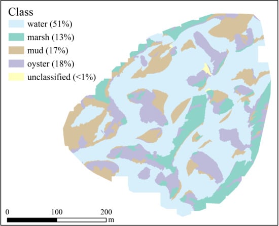
The use of the selected variables as inputs for the standard nearest neighbor classification in eCognition resulted in the habitat map presented in Figure 7. Overall, 51% (59,691 m2) of the surveyed area was classified as water, 13% (15,195 m2) as marsh habitat, 18% (20,858 m2) was classified as oysters, and 17% (20,010 m2) as mud. Less than 1% (254 m2) was left unclassified. The final ruleset was saved as a file within eCognition and is available in Supplementary Materials; it can be used by anyone who has access to the software.
The confusion matrix of the classification is presented in Table 2. An overall accuracy of 79% was achieved for the classification, with a Kappa coefficient of 0.72. Table 2 also displays the producer’s and user’s accuracies. Producer’s accuracy is a measure of the error of omission, identifying how often real features are represented in the classification [43,44]. Oyster and water demonstrated high producer’s accuracies, indicating that areas of oyster and water were infrequently excluded from their respective classes. User’s accuracy is a measure of the error of commission, measuring how often objects are erroneously included in a class [43,44]. Mud and marsh had a high user’s accuracy, indicating that these classes are reliable for the end user.
4. Discussion
4.1. GEOBIA Classification
The GEOBIA classification produced promising results that suggest the technique can be used to monitor relative changes in intertidal habitat cover. Between the three intertidal habitat covers, most misclassifications occurred between the oyster and marsh habitats, which can be explained by the lower separation represented in the difference matrix of the three habitat classes. Future research can further emphasize the textural characteristics to better differentiate oysters and marsh, or topographical characteristics such as rugosity, which is a measure of the local variation in a surface’s height [45]. However, we note that this may remain challenging as these two habitat types often spatially overlap and create mixed, transitional areas. In areas of high marsh, for instance, oysters may be partially or entirely obscured in UAS imagery. In cases with integrated habitat patches, fuzzy logic and classifications may be more representative of natural transitional zones than traditional techniques that can oversimplify complex systems by imposing discrete boundaries to habitats [46]. The area that demonstrated the most difficulty in differentiating habitats was the eastern border of the scene, which is composed of marsh habitats. This is likely due in part to the artificially smooth edges on the scene’s border, which bias geometric features that are used in the classification.
GEOBIA works more like the human mind than traditional pixel-based techniques as it allows for the classification of distinct, meaningful objects, rather than uniform pixels. eCognition provides valuable tools to identify variables that separate classes from one another and goes beyond the value of a layer, allowing for the exploration of standard deviations, maximums, minimums, and modes of spectral layers as well as geometric or textural attributes. For example, the standard deviation of all three spectral bands identified an upper threshold that separated mud from marsh and oyster. The lower standard deviation demonstrates how mud is a more homogenous land cover than the other two habitats, and it is the exploration of these attributes that allows for a more informed classification. Features such as standard deviation and average elevation could have been assigned upper and lower thresholds for classes to produce a higher accuracy, but this would have limited the generality and replicability of the ruleset, which we intended to be applicable to any other study site. We note, however, that while this study aimed to produce a general and replicable ruleset that is as automated as possible, it may be useful for end-users to adapt the ruleset provided in Supplementary Materials to make it more specific for the monitoring of a particular site.
While developing a GEOBIA workflow requires significant time in data exploration, one benefit lies within the repeatability of the ruleset if data are collected at the same site multiple times. While it is repeatable, there are initial considerations as several inputs and variables can be used to achieve similar success. For example, local rugosity measured by the variation in elevation at a 3 × 3 window size could have served as an edge detection input as it outlined habitats well and the values were low over the smooth water regions. One of the primary decisions in GEOBIA is selecting which layers serve as initial inputs, but this is in part facilitated by the use of feature-space optimization.
4.2. Limitations and Considerations
Despite promising results, there are some notable shortcomings of the GEOBIA workflow outlined. The water masking had difficulty differentiating between mudflats that were partially inundated and contiguous areas of water. A few small patches of oysters were also misclassified as water, while the more extensive reefs demonstrated no misclassifications in the masking step. This may be remedied by using a finer scale when segmenting the scene, but this comes with its tradeoffs (e.g., processing time). Like mud, water is homogenous in texture and spectral variability, making the delineation challenging.
An important consideration when studying morphology is the scale of analysis. During the data exploration stage, we conducted a multi-scale analysis in which samples of each habitat type were selected and local terrain attributes such as rugosity and relative position were calculated at a spectrum of scales ranging from the resolution of the imagery (0.66 cm) to multiple meters. While some signatures provided a level of separation between habitats, the classification was not improved when this information was input into the GEOBIA workflow. The role of scale and multiscale variables should be further explored as some variables that seemingly provide no information on differentiating classes may be relevant at larger or smaller windows of analysis that better capture the structural patterns of habitats [47,48], especially considering the fine spatial resolution that is now attainable with UASs.
There are also important considerations regarding the collection of imagery such as time of day, cloud cover, and the effect of shadows [49]. Collecting images on overcast days can aid in minimizing shadows [50]. Wind conditions also affect imagery collection as high winds can be detrimental to the stability of the UAS, and therefore the quality of images. Additionally, wind can cause waves that may alter the spectral response of the habitats by spraying them. Conditions should be kept as constant as possible when surveying a site as part of a time series dataset. In addition to atmospheric conditions, working in an intertidal environment poses challenges with establishing ground control points and checkpoints. The American Society for Photogrammetry and Remote Sensing recommends 20 horizontal and vertical checkpoints for areas less than 500 square km [51]. Due to the challenges of sampling this environment, our only checkpoints were the four ground control targets. While this limitation is not of great concern given our objective of characterizing relative coverage, this becomes a more significant concern if this workflow was to be used for temporal monitoring.
Another consideration is the computing capabilities necessary to conduct this analysis efficiently, as processing these data is computationally intensive. Details on the computation time and hardware used in processing can be found in Appendix A. Additionally, there are few open-source solutions that allow the same capabilities as a software suite such as eCognition. As open-source options for GEOBIA advance, this process will become even less cost-intensive. Researchers have used a Python-based open-source workflow for GEOBIA [52], highlighting the growing capabilities of open-source solutions.
4.3. Future Directions
There is potential for future studies to improve upon classification accuracies by collecting imagery from different spectral bands. This study aimed to minimize costs as much as possible and as a result, selected to use only RGB imagery. However, if available, near-infrared imagery could be utilized for more accurate water classifications. A higher spectral resolution may also aid in differentiating oysters and marsh, which caused the most misclassifications for reefs.
The spatial resolution of this dataset allows for analysis within a reef system itself. While developing accurate distributions of oyster reefs is valuable to assess change over time, analyzing the structure of a thriving reef is also an essential component. This is particularly relevant in areas such as the Big Bend of Florida where reef collapse can lead to an increase in reef extent as broken shells get dispersed [12]. While reefs are increasing in extent, the availability of a stable substrate for larvae is decreasing [12]. The NOAA Oyster Restoration Workgroup suggests monitoring metrics such as population structure, recruitment, disease, and vertical relief of oyster reefs to provide a more complete outlook on the health of reefs and populations [7,12]. UASs can provide informative data on these metrics, the most direct application being vertical relief and morphology, which has been conducted successfully for eastern oyster reefs in other areas such as off the coast of North Carolina, USA [19].
As reefs continue to erode due to anthropogenic and environmental stressors, there is often a concentrated restoration effort in regions losing reefs such as in the Big Bend of Florida. Restoration often involves installing a hard substrate for the oysters to settle on including boulders and recycled oyster shells [53]. These restoration activities are typically conducted in areas where reefs used to exist. However, given a changing environment, these may not be the ideal areas today, emphasizing the importance of current information regarding where extant oyster reefs are and are not as well as the structural integrity of these reefs. The multi-scale capabilities of this workflow not only allow for the selection of sites where reefs can be successful, but also enable the characterization of a thriving reef’s structure.
5. Conclusions
Developing an expedient workflow to monitor coastal environments is essential as stressors continue to alter coastal systems. As we continue to extract and divert water resources, estuarine systems that are reliant on freshwater inflow are of particular concern. Remote sensing techniques can cut the costs and time of monitoring these ecosystems, and UASs present an accessible alternative to traditional methods or less precise and broader-scale satellite imagery. The composition of coastal ecosystems is unique and dynamic, again highlighting the benefit of UASs as a tool because they can collect localized data to analyze the complexities of specific sites. Morphology, hydrodynamics, and coastal development are all influencing factors on how these habitats expand or decline, and UASs can efficiently capture data to document changes.
Our study showed that UAS imagery paired with GEOBIA could inform management by quantifying the relative coverage of different coastal habitat types. Designing a GEOBIA ruleset that is specific to a study site allows for a high level of repeatability, making long-term monitoring more feasible at a given site. This workflow can be extended to other areas of Florida’s Big Bend coastline to monitor changes. The GEOBIA workflow we developed incorporated specific steps such as the water masking step to address difficulties with classifications in an intertidal environment that has little spectral separability between habitats. Connecting changes in habitats by using quantifiable measurements such as reef morphology or changes in area can inform restoration efforts and identify areas prone to shoreline erosion. Understanding which spatiotemporal variables contribute to reef success can provide valuable information to restoration and monitoring efforts alike. While coastal research using UASs is gaining momentum, the procedure is just as important as the mechanism, and GEOBIA serves as a streamlined approach to classify coastal habitats and quantify changes.
Supplementary Materials
The following are available online at https://www.mdpi.com/2072-4292/12/4/677/s1.
Author Contributions
Conceptualization, V.L. and M.C.E.; Methodology, M.C.E.; and V.L.; Validation, M.C.E.; Formal analysis, M.C.E.; Resources, P.C.F. and V.L.; Writing—original draft preparation, M.C.E.; Writing—review and editing, V.L., P.C.F., B.W., and E.V.C.; Visualization, M.C.E.; and V.L.; Supervision, V.L., P.C.F., B.W., and E.V.C.; Funding acquisition, V.L. All authors have read and agreed to the published version of the manuscript.
Funding
This research was funded by a Gulf Research Program Early-Career Research Fellowship awarded to V. Lecours by the National Academies of Sciences, Engineering, and Medicine. We also acknowledge the support of the University of Florida College of Agricultural and Life Sciences through an assistantship to M. Espriella. Publication of this article was funded in part by the University of Florida Open Access Publishing Fund.
Acknowledgments
Thanks are due to Steve Beck, Sean Denney, Lindsey Garner, and Andrew Ortega who led the UAS imagery and RTK data collection.
Conflicts of Interest
The authors declare no conflicts of interest. The funders had no role in the design of the study; in the collection, analyses, or interpretation of data; in the writing of the manuscript, or in the decision to publish the results.
Appendix A

Table A1.
Description of object features used in the feature-space optimization and their corresponding descriptions adapted from the eCognition reference book and Bialas 2015.
Table A1.
Description of object features used in the feature-space optimization and their corresponding descriptions adapted from the eCognition reference book and Bialas 2015.
| Object Feature | Description |
|---|---|
| Asymmetry | A measure of the variance in the x-direction and y-direction of an approximated ellipse around the object |
| Border index | Measures how jagged an object is; border length of object compared to border length of smallest enclosing rectangle |
| Brightness Index 1 | ((R2 + G2 + B2)/3)0.5 |
| Compactness | Product of the length and width, divided by the number of pixels |
| Density | Describes distribution in space of the pixels in an object; number of pixels forming object divided by its radius |
| Elliptic fit | Measures what falls inside versus outside an ellipse with the same length and width of and object |
| Green leaf index 4 | (2G − R − B)/(2G + R + B) |
| Hue index 1 | (2 * R − G − B)/(G − B) |
| Length/width | The length of the object divided by the width |
| Main direction | The direction of the eigenvector belonging to the larger of the two eigenvalues |
| Max difference | The maximum difference between mean values for layers of an object divided by the brightness of the respective objects |
| Mean blue | Mean reflectance of the blue band of all pixels in an object |
| Mean brightness | Mean brightness of all pixels in an object |
| Mean DSM | Mean elevation of all pixels in an object in the DSM layer |
| Mean green | Mean reflectance of the green band of all pixels in an object |
| Mean red | Mean reflectance of the red band of all pixels in an object |
| Normalized green red difference index 2 | (G − R)/(G + R) |
| Number of neighbors | Number of neighbors in which an object shares a common border |
| Radius of largest enclosed ellipse | Measures an object’s similarity to an ellipse; ratio of largest enclosed ellipse radius to the radius of an ellipse with the same area as the object |
| Radius of smallest enclosing ellipse | How much of an object is similar to an ellipse; ratio of smallest enclosing ellipse radius to radius of and ellipse with the same area as the object |
| Rectangular fit | Describes how well an object fits into a rectangle of similar size; are of image object inside versus outside a rectangle that has the same length and width as the object |
| Redness Index 1 | R2/(B*G3) |
| Relative border to image border | Border length an object shares with outer boundary of entire image |
| Roundness | Describes how similar an object is to an ellipse; difference of enclosing ellipse and enclosed ellipse |
| Shape index | Shape complexity; border length |
| Spectral slope 2 | (R − B)/(R + B) |
| Standard deviation blue | Standard deviation of blue band reflectance values over all pixels in an object |
| Standard deviation brightness | Standard deviation of the brightness values over all pixels in an object |
| Standard deviation DSM | Standard deviation of elevation values over all pixels in an object |
| Standard deviation green | Standard deviation of green band reflectance values over all pixels in an object |
| Standard deviation red | Standard deviation of red band reflectance values over all pixels in an object |
| Standard deviation of length of edges | Measures how lengths of edges deviate from mean value |
| Vegetation index 3 | (B + R − G)/(B + R + G) |
| Water index 3 | (R − B + G)/(B + R + G) |
1 Spectral indices from Mandal (2016) input into eCognition as arithmetic features; 2 Spectral indices from Tucker (1979) input into eCognition as arithmetic features; 3 Spectral indices from Upadhyay (2016) input into eCognition as arithmetic features; 4 Spectral indices from Louhaichi (2001) input into eCognition as arithmetic features.
Figure A1.
Orthomosaic and DSM following the water masking step.

Table A2.
Hardware and processing time for image processing conducted in Pix4D.
| Description | |
|---|---|
| CPU | Intel Xeon CPU E5-2630 v4 2.20 GHz |
| RAM | 192 GB |
| GPU | NVIDIA Quadpro P4000 |
| Initial processing time (image calibration, finding keypoints) | 1 h 37 min |
| Point cloud densification | 5 h 25 min |
| DSM generation | 2 h 17 min |
| Orthomosaic generation | 1 h 37 min |
| Total processing time | 10 h 56 min |
Table A3.
Hardware and processing time for image processing conducted in eCognition.
| Description | |
|---|---|
| CPU | Intel Xeon Silver 4114 2.20 GHz 2.19 GHz (2 processors) |
| RAM | 256 GB |
| GPU | NVIDIA Quadpro P60000 |
| Segmentation | 2 h |
| Feature-space optimization | 3+ h |
| Classification | 2 h 5 min |
| Exporting results | 5 min |
| Total processing time | 7+ h |
References
- Seavey, J.R.; Pine, W.E., III; Frederick, P.C.; Sturmer, L.; Berrigan, M. Decadal changes in oyster reefs in the Big Bend of Florida’s Gulf Coast. Ecosphere 2011, 2. [Google Scholar] [CrossRef]
- Beck, M.W.; Brumbaugh, R.D.; Airoldi, L.; Carranza, A.; Coen, L.D.; Crawford, C.; Defeo, O.; Edgar, G.J.; Hancock, B.; Kay, M.C.; et al. Oyster reefs at risk and recommendations for conservation, restoration, and management. BioScience 2011, 61, 107–116. [Google Scholar] [CrossRef] [Green Version]
- Coen, L.D.; Brumbaugh, R.D.; Bushek, D.; Grizzle, R.; Luckenback, M.W.; Posey, M.H.; Powers, S.P.; Tolley, S.G. Ecosystem services related to oyster restoration. Mar. Ecol. Prog. Ser. 2007, 341, 303–307. [Google Scholar] [CrossRef]
- Scyphers, S.B.; Powers, S.P.; Heck, K.L., Jr.; Byron, D. Oyster reefs as natural breakwaters mitigate shoreline loss and facilitate fisheries. PLoS ONE 2011, 6. [Google Scholar] [CrossRef]
- Tolley, S.G.; Volety, A.K.; Savarese, M. Influence of salinity on the habitat use of oyster reefs in three southwest Florida estuaries. J. Shellfish Res. 2005, 24, 127–137. [Google Scholar] [CrossRef]
- Shepard, C.C.; Crain, C.M.; Beck, M.W. The protective role of coastal marshes: A systematic review and meta-analysis. PLoS ONE 2011, 6. [Google Scholar] [CrossRef]
- Geselbracht, L.; Freeman, K.; Kelly, E.; Gordon, D.R.; Putz, F.E. Retrospective and prospective model simulations of sea level rise impacts on Gulf of Mexico coastal marshes and forests in Waccasassa Bay, Florida. Clim. Chang. 2011, 107, 35–57. [Google Scholar] [CrossRef] [Green Version]
- Raabe, E.A.; Stumpf, R.P. Expansion of tidal marsh in response to sea-level rise: Gulf Coast of Florida, USA. Estuaries Coasts 2016, 39, 145–157. [Google Scholar] [CrossRef]
- Krauss, K.W.; From, A.S.; Doyle, T.W.; Doyle, T.J.; Barry, M.J. Sea-level rise and landscape change influence mangrove encroachment onto marsh in the Ten Thousand Islands region of Florida, USA. J. Coast Conserv. 2011, 15, 629–638. [Google Scholar] [CrossRef]
- Frederick, P.C.; Vitale, N.; Pine, W.E., III; Seavey, J.R. Reversing a rapid decline in oyster reefs: Effects of durable substrate on oyster populations, elevations, and aquatic bird community composition. J. Shellfish Res. 2016, 35, 359–367. [Google Scholar] [CrossRef]
- Kaplan, D.A.; Oblabarrieta, M.; Frederick, P.C.; Valle-Levinson, A. Freshwater detention by oyster reefs: Quantifying a keystone ecosystem service. PLoS ONE 2016, 11. [Google Scholar] [CrossRef] [PubMed]
- Radabaugh, K.R.; Geiger, S.P.; Moyer, P.P. Oyster Integrated Mapping and Monitoring Program Report for the State of Florida; FWRI Technical Report No. 22; Fish and Wildlife Research Institute, Florida Fish and Wildlife Conservation Commission: St. Petersburg, FL, USA, 2019. [Google Scholar]
- Florida Fish and Wildlife Conservation Commission. Available online: https://myfwc.com/research/saltwater/fishstats/commercial-fisheries/landings-in-florida/ (accessed on 21 October 2019).
- Camp, E.V.; Pine, W.E., III; Havens, K.; Kane, A.S.; Walters, C.J.; Irani, T.; Lindsey, A.B.; Morris, J.G., Jr. Collapse of a historic oyster fishery: Diagnosing causes and identifying paths toward increase resilience. Ecol. Soc. 2015, 20. [Google Scholar] [CrossRef]
- North, E.W.; King, D.M.; Xu, J.; Hood, R.R.; Newell, R.I.E.; Paynter, K.; Kellogg, M.L.; Liddel, M.K.; Boesch, D.F. Linking optimization and ecological models in a decision support tool for oyster restoration and management. Ecol. Appl. 2010, 20, 851–866. [Google Scholar] [CrossRef] [PubMed]
- Banks, P.; Beck, S.; Chapiesky, K.; Isaacs, J. Lousiana Oyster Fishery Management Plan; Louisiana Department of Wildlife and Fisheries Technical Report; Louisiana Department of Wildlife and Fisheries, Office of Fisheries: Baton Rouge, LA, USA, 2016; 214p. [Google Scholar]
- North Carolina Environmental Quality. Available online: http://portal.ncdenr.org/web/mf/habitat/enhancement/oyster-sanctuaries (accessed on 19 November 2019).
- Byers, J.E.; Grabowski, J.H.; Piehler, M.F.; Hughes, R.A.; Weiskel, H.W.; Malek, J.C.; Kimbro, D.L. Geographic variation in intertidal oyster reef properties and the influence of tidal prism. Limnol. Oceanogr. 2015, 60, 1051–1063. [Google Scholar] [CrossRef]
- Windle, A.E.; Poulin, S.K.; Johnston, D.W.; Ridge, J.T. Rapid and accurate monitoring of intertidal oyster habitat using unoccupied aircraft systems and structure from motion. Remote Sens. Environ. 2019, 11, 2394. [Google Scholar] [CrossRef] [Green Version]
- Grizzle, R.; Ward, K.; Geselbracht, L.; Birch, A. Distribution and condition of intertidal eastern oyster (Crassostrea virginica) reefs in Apalachicola Bay Florida based on high-resolution satellite imagery. J. Shellfish Res. 2018, 37, 1–12. [Google Scholar] [CrossRef]
- Escapa, M.; Isacch, J.P.; Daleo, P.; Alberti, J.; Iribarne, O.; Borges, M.; Dos Santos, E.P.; Gagliardini, D.A.; Lasta, M. The distribution and ecological effects of the introduced pacific oyster Crassostrea gigas (Thunberg, 1793) in northern Patagonia. J. Shellfish Res. 2004, 3, 765–772. [Google Scholar]
- Colomina, I.; Molina, P. Unmanned aerial systems for photogrammetry and remote sensing: A review. ISPRS J. Photogramm. Remote Sens. 2014, 92, 79–97. [Google Scholar] [CrossRef] [Green Version]
- Hay, G.J.; Castilla, G. Geographic object-based image analysis (GEOBIA): A new name for a new discipline. In Lecture Notes in Geoinformation and Cartography; Springer: Berlin, Germany, 2008; pp. 75–89. [Google Scholar] [CrossRef]
- Blaschke, T. Object based image analysis for remote sensing. ISPRS J. Photogramm. Remote Sens. 2010, 65, 2–16. [Google Scholar] [CrossRef] [Green Version]
- Gibbes, C.; Sanchayeeta, A.; Rostant, L.; Southworth, J.; Qiu, Y. Application of object based classification and high resolution satellite imagery for savanna ecosystem analysis. Remote Sens. Environ. 2010, 2, 2748–27772. [Google Scholar] [CrossRef] [Green Version]
- Moskal, L.M.; Styers, D.M.; Halabisky, M. Monitoring urban tree cover using object-based image analysis and public domain remotely sensed data. Remote Sens. Environ. 2011, 3, 2243–2262. [Google Scholar] [CrossRef] [Green Version]
- Pande-Chhetri, R.; Abd-Elrahman, A.; Liu, T.; Morton, J.; Wilhelm, V.L. Object-based classification of wetland vegetation using very high-resoultion unmanned air system imagery. Eur. J. Remote Sens. 2017, 50, 564–576. [Google Scholar] [CrossRef] [Green Version]
- Diesing, M.; Green, S.L.; Stephens, D.; Lark, R.M.; Stewart, H.A.; Dove, D. Mapping seabed sediments: Comparison of manual, geostatistical, object-based image analysis and machine learning approaches. Cont. Shelf Res. 2014, 84, 107–119. [Google Scholar] [CrossRef] [Green Version]
- Florida Fish and Wildlife Conservation Commission. Available online: http://geodata.myfwc.com/datasets/oyster-beds-in-florida (accessed on 5 August 2019).
- NOAA Tides & Currents. Available online: https://tidesandcurrents.noaa.gov/stations.html?type=Water+Level+Reports (accessed on 4 November 2019).
- Frey, J.; Kovach, K.; Stemmler, S.; Kock, B. UAV photogrammetry of forests as a vulnerable process. A sensitivity analysis for a structure from motion RGB-image pipeline. Remote Sens. Environ. 2018, 10, 912. [Google Scholar] [CrossRef] [Green Version]
- Pix4D Mapper [computer software]. Available online: https://www.pix4d.com/product/pix4dmapper-photogrammetry-software (accessed on 18 January 2019).
- ESRI ArcGIS Pro v 2.4 [computer software]. Available online: https://pro.arcgis.com/es/pro-app (accessed on 8 July 2019).
- eCognition Developer 9 [computer software]. Available online: http://www.ecognition.com/suite/ecognition-developer (accessed on 15 July 2019).
- Upadhyay, P.; Mahadik, S.; Kamble, A. Image classification using visible RGB bands. In Proceedings of the International Conference on Computing for Sustainable Global Development, New Delhi, India, 16 March 2016. [Google Scholar]
- Louhaichi, M.; Borman, M.M.; Johnson, D.E. Spatially located platform and aerial photography for documentation of grazing impacts on wheat. Geocarto Int. 2001, 16, 65–70. [Google Scholar] [CrossRef]
- Mandal, U.K. Spectral color indices based geospatial modeling of soil organic matter in Chitwan District, Nepal. In Proceedings of the ISPRS Congress, Prague, Czech Republic, 12 July 2019. [Google Scholar]
- Tucker, C.J. Red and photographic infrared linear combinations for monitoring vegetation. Remote Sens. Environ. 1979, 8, 127–150. [Google Scholar] [CrossRef] [Green Version]
- Bialas, J. Object-Based Classification of Earthquake Damage from High-Resolution Optical Imagery Using Machine Learning. Master’s Thesis, Michigan Technological University, Houghton, MI, USA, 2015. [Google Scholar]
- Jensen, J.R. Introductory Digital Image Processing: A Remote Sensing Perspective, 3rd ed.; Pearson Education: Upper Saddle River, NJ, USA, 2005. [Google Scholar]
- Totora, R.D. A note on sample size estimation for multinomial populations. Am. Stat. 1978, 321, 1001–1002. [Google Scholar]
- Congalton, R.G. A review of assessing the accuracy of classifications of remotely sensed data. Remote Sens. Environ. 1991, 37, 35–46. [Google Scholar] [CrossRef]
- Fung, T.; LeDrew, E. The determination of optimal threshold levels for change detection using various accuracy indices. Photogramm. Eng. Remote Sens. 1988, 54, 1449–1454. [Google Scholar]
- Story, M.; Congalton, R.G. Accuarcy assessment: A user’s perspective. Photogramm. Eng. Remote Sens. 1986, 52, 397–399. [Google Scholar]
- Lecours, V.; Dolan, M.F.J.; Micallef, A.; Lucieer, V. A review of geomorphometry, the quantitative study of the seafloor. Hydrol. Earth Syst. Sc. 2016, 20, 3207–3244. [Google Scholar] [CrossRef] [Green Version]
- Fiorentino, D.; Lecours, V.; Brey, T. On the art of classification in spatial ecology: Fuzziness as an alternative for mapping uncertainty. Front. Ecol. Evol. 2018, 6. [Google Scholar] [CrossRef] [Green Version]
- Lecours, V.; Devillers, R.; Schneider, D.C.; Lucieer, V. Spatial scale and geographic context in benthic habitat mapping: Review and future directions. Mar. Ecol. Prog. Ser. 2015, 535, 259–284. [Google Scholar] [CrossRef] [Green Version]
- Misiuk, B.; Lecours, V.; Bell, T. A multiscale approach to mapping seabed sediments. PLoS ONE 2018, 13. [Google Scholar] [CrossRef] [PubMed] [Green Version]
- Patterson, C.; Koski, W.; Pace, P.; McLuckie, B.; Bird, D.M. Evaluation of an unmanned aircraft system for detecting surrogate caribou targets in Labrador. J. Unmanned Veh. Syst. 2015, 4, 53–69. [Google Scholar] [CrossRef] [Green Version]
- Barnas, A.F.; Darby, B.J.; Vandeberg, G.S.; Rockwell, R.F.; Ellis-Felege, S.N. A comparison of drone imagery and ground-based methods for estimating the extent of habitat destruction by lesser snow geese (Anser caerulescens caerulescens) in La Pérouse Bay. PLoS ONE 2019, 14. [Google Scholar] [CrossRef] [Green Version]
- American Society for Photogrammetry and Remote Sensing. ASPRS accuracy standards for digital geospatial data. Photogramm. Eng. Remote Sens. 2015, 81, A1–A26. [Google Scholar] [CrossRef]
- Clewley, D.; Bunting, P.; Shepherd, J.; Gillingham, S.; Flood, N.; Dymond, J.; Lucas, R.; Armston, J.; Moghaddam, M. A Python-based open source system for geographic object-based image analysis (GEOBIA) utilizing raster attribute tables. Remote Sens. Environ. 2014, 6, 6111–6135. [Google Scholar] [CrossRef] [Green Version]
- Brumbaugh, R.D.; Coen, L.D. Contemporary approaches for small-scale oyster reef restoration to address substrate versus recruitment limitation: A review and comments relevant for the olympia oyster, Osrea lurida carpenter 1864. J. Shellfish Res. 2009, 28, 147–161. [Google Scholar] [CrossRef]
Figure 1.
The area within the red rectangle represents Florida’s Big Bend coastline. The black dot represents the approximate location of the study site.
Figure 1.
The area within the red rectangle represents Florida’s Big Bend coastline. The black dot represents the approximate location of the study site.

Figure 2.
This historical footprint of eastern oyster reefs near Cedar Key, Florida, USA is the most comprehensive oyster reef map available of the area. Reefs are not represented to scale.
Figure 2.
This historical footprint of eastern oyster reefs near Cedar Key, Florida, USA is the most comprehensive oyster reef map available of the area. Reefs are not represented to scale.

Figure 3.
(A) Mudflat, (B) salt marsh with fringing oysters, and (C) intertidal oyster reef habitats. Images were taken from a UAS at Little Trout Creek.
Figure 3.
(A) Mudflat, (B) salt marsh with fringing oysters, and (C) intertidal oyster reef habitats. Images were taken from a UAS at Little Trout Creek.

Figure 4.
Workflow diagram detailing imagery and geographic object-based image analysis processing.

Figure 5.
Orthomosaic (left) and digital surface model (right) developed from the collected imagery. The yellow triangles on the orthomosaic represent the placement of ground targets. Difficulties with finding image matching points resulted in some artifacts over water in the digital surface model because of the extensive interpolation.

Figure 6.
Laplacian filter (left) used for edge detection with a detailed section (top right) and its corresponding area on the orthomosaic (bottom right). The red rectangle represents the extent of the detailed section.
Figure 6.
Laplacian filter (left) used for edge detection with a detailed section (top right) and its corresponding area on the orthomosaic (bottom right). The red rectangle represents the extent of the detailed section.

Figure 7.
Habitat map produced from the standard nearest neighbor classification.

Table 1.
Object features that allow for the most separation in classes at each dimension with the corresponding separation value. Dimension refers to the number of object features contributing to the separation analysis. The higher the separation value, the greater the differentiation between the classes as represented by the randomly selected samples.
| Dimension | Separation | Object Features |
|---|---|---|
| 1 | 0.108 | water index |
| 2 | 0.469 | water index, standard deviation green |
| 3 | 0.855 | water index, standard deviation red, main direction |
| 4 | 1.117 | water index, standard deviation red, main direction, asymmetry |
| 5 | 1.517 | water index, standard deviation green, main direction, asymmetry, vegetation index |
| 6 | 1.684 | water index, standard deviation red, main direction, asymmetry, vegetation index, standard deviation blue |
| 7 | 1.835 | water index, standard deviation red, main direction, asymmetry, vegetation index, standard deviation blue, max difference |
| 8 | 2.028 | water index, standard deviation red, main direction, asymmetry, vegetation index, standard deviation blue, max difference, radius of largest enclosed ellipse |
| 9 | 2.173 | water index, standard deviation red, main direction, asymmetry, vegetation index, standard deviation blue, max difference, radius of largest enclosed ellipse, spectral slope |
| 10 | 2.257 | water index, standard deviation red, main direction, asymmetry, vegetation index, standard deviation blue, max difference, radius of largest enclosed ellipse, spectral slope, border index |
Table 2.
Confusion matrix of the actual and classified habitat covers with the accuracy of results. UA = user’s accuracy PA = producer’s accuracy, and OA = overall accuracy.
Table 2.
Confusion matrix of the actual and classified habitat covers with the accuracy of results. UA = user’s accuracy PA = producer’s accuracy, and OA = overall accuracy.
| Actual | ||||||
| Oyster | Marsh | Mud | Water | UA (%) | ||
| Oyster | 133 | 33 | 14 | 6 | 71.51 | |
| Marsh | 17 | 130 | 2 | 1 | 86.67 | |
| Classified | Mud | 6 | 3 | 119 | 17 | 82.07 |
| Water | 10 | 0 | 31 | 142 | 77.60 | |
| PA (%) | 80.12 | 78.31 | 71.69 | 85.54 | ||
| OA (%) Kappa | 78.92 0.72 |
© 2020 by the authors. Licensee MDPI, Basel, Switzerland. This article is an open access article distributed under the terms and conditions of the Creative Commons Attribution (CC BY) license (http://creativecommons.org/licenses/by/4.0/).
Share and Cite
MDPI and ACS Style
Espriella, M.C.; Lecours, V.; C. Frederick, P.; V. Camp, E.; Wilkinson, B. Quantifying Intertidal Habitat Relative Coverage in a Florida Estuary Using UAS Imagery and GEOBIA. Remote Sens. 2020, 12, 677. https://doi.org/10.3390/rs12040677
AMA Style
Espriella MC, Lecours V, C. Frederick P, V. Camp E, Wilkinson B. Quantifying Intertidal Habitat Relative Coverage in a Florida Estuary Using UAS Imagery and GEOBIA. Remote Sensing. 2020; 12(4):677. https://doi.org/10.3390/rs12040677
Chicago/Turabian StyleEspriella, Michael C., Vincent Lecours, Peter C. Frederick, Edward V. Camp, and Benjamin Wilkinson. 2020. "Quantifying Intertidal Habitat Relative Coverage in a Florida Estuary Using UAS Imagery and GEOBIA" Remote Sensing 12, no. 4: 677. https://doi.org/10.3390/rs12040677
Note that from the first issue of 2016, this journal uses article numbers instead of page numbers. See further details here.