Insect Target Classes Discerned from Entomological Radar Data

Abstract

Entomological radars employing the ‘ZLC’ (zenith-pointing linear-polarized narrow-angle conical scan) configuration detect individual insects flying overhead and can retrieve information about a target’s trajectory (its direction and speed), the insect’s body alignment and four parameters that characterize the target itself: its radar cross section, two shape parameters and its wingbeat frequency. Criteria have previously been developed to distinguish Australian Plague Locusts Chortoicetes terminifera, large moths, medium moths and small insects using the target-character parameters. Combinations of target characters that occur frequently, known as target ‘classes’, have also been identified previously both through qualitative analyses and more objectively with a 4D peak-finding algorithm applied to a dataset spanning a single flight season. In this study, fourteen years of radar observations from Bourke, NSW (30.0392°S, 145.952°E, 107 m above MSL) have been used to test this approach and potentially improve its utility. We found that the previous criteria for assigning targets to classes require some modification, that classes identified in the previous studies were frequently present in other years and that two additional classes could be recognized. Additionally, by incorporating air-temperature information from a meteorological model, we have shown that different classes fly in different temperature ranges. By drawing on knowledge concerning migrant species found in the regional areas around the radar site, together with morphological measurements and radar cross-section data for proxy species, we have made tentative identifications of the insect taxa likely to be contributing to each class.

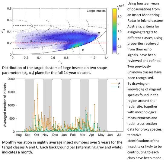
1. Introduction

Over the past five decades, there has been dramatic progress in the technical development of radar entomology and this has contributed greatly to developing an understanding of insect migratory behavior and its ecological consequences [1]. Since the late 1990s, autonomously operating vertical-beam radars transmitting at X-band (9.4 GHz, 3.2 cm wavelength) and employing the ‘ZLC’ configuration (zenith-pointing linear-polarized narrow-angle conical scan) and known variously as VLRs (vertical-looking radars) and IMRs (insect monitoring radars), have been widely adopted [2,3] and this technology continues to develop [4].

Datasets extending over several years and with millions of individual insect traverses through the radar beam have now accumulated at sites in different locations around the world and have provided the basis for several studies of migratory insects (e.g., References [2,5,6]). In 1998, an IMR was installed at Bourke airport, New South Wales (30.0392°S, 145.952°E, 107 m above MSL) and has operated, with some gaps, up to the present. A second unit was operated at Thargomindah airport, Queensland (27.9864°S, 143.811°E, 132 m above MSL) from 1999–2013 [7]. As well as accumulating research data, these two radars have played an operational role: the observations are routinely accessed by the Australian Plague Locust Commission (APLC) to support its decision-making and to recognize patterns in the development, spread and persistence of locust outbreaks [8].

Determining the types of targets that produce the echoes detected by a radar has been a persistent challenge for radar entomologists. ZLC radar represented a significant advance, as these units provide a consistent measure of radar cross section (RCS; the ventral aspect polarization-averaged RCS, a₀, which can be used to estimate target mass [9]) and two measures of target shape (α₂ and α₄ or alternatively σ_xx and σ_yy) [10]. We have eliminated targets with large sizes (RCS > 5 cm²) as these are probably birds; these made up only a small proportion of the total. Moreover, it was later shown that a fourth character, the wingbeat frequency f_w, could be retrieved for at least some echoes [11]. Discrimination between different insect taxa would allow species that are not of interest to be excluded, enabling significantly more precise biological analyses by researchers, pest managers and other potential users. Size (transformed into an estimate of mass) has been used to identify targets detected by ZLC radars in Europe [12,13,14]. In studies of two noctuid moths (the Silver Y, Autographa gamma and the Large Yellow Underwing, Noctua pronuba, sphingid moths and butterflies [15], echo selection was based primarily on the radar-estimated size of the targets (

Table A1. Mass and radar cross section (RCS) measurements used to set target-selection criteria in previous radar studies.

	N	Mean (mg)	Std (mg)	Range (mg)	σxx/σyy
Noctuid moths
Autographa gamma [44]	11	146	35	111–181
Noctua pronuba [15]	33	344	66	300–500
Sphingid moths
Agrius convolvuli [15]	1	1212		600–1500 1
Sphinx igustri [15]	7	1256	146
Laothoe populi [15]	18	658	155
Deilephila elpenor [15]	13	595	68
Hyloicus pinastri [15]	5	571	164
Nymphalid butterflies
Vanessa atalanta [15]	7	272	60	100–400 2
Vanessa cardui [15]	17	192	56
Ladybird beetles
Harmonia axyridis and Coccinella septempunctata [13]	20/10	-	-	25–42 2	1.5–4.1
Hoverflies
Episyrphus balteatus and Eupeodes corollae [14]	18	22.3	6.6	15–28 2	5–10

¹ The mass range applies to all five sphingid species. ² The mass range applies to both species.

). Aerial netting and light-trap catches provided supporting evidence. For butterflies, for example, selection was based on flying times (hours of the day, days of the year) as well as size [15]. The shape parameters have also been used to identify targets. In Europe, ladybirds and hoverflies were selected by using the ratio σ_xx/σ_yy (where σ_xx is the RCS when polarization is aligned with the body axis and σ_yy the RCS perpendicular to this), in combination with mass [13,14]. Wingbeat frequency has long been used to make inferences about the species forming a target population [16] but only the IMR radars employed in Australia have routinely provided it for individual targets for which size, shape and trajectory information is also available [11].

In recent studies based on the Australian IMR dataset, size, shape and wingbeat frequency were used to identify echoes from Australian Plague Locusts Chortoicetes terminifera [8]. The criteria used (

Table A2. Previous radar-target-class selection criteria for the Australian Plague Locust C. terminifera, large moths, medium moths and small insects [22]. The size parameter a₀ of the target, one of the two shape parameters α₄ and the fundamental or wingbeat frequency f_w are used to classify the radar targets. Note there is no selection on α₂ values.

Target	a0 (cm2)	α4	fw (Hz)	Mass (mg)
	(~0.001–~10 cm2)	(0–~0.5)	(0–~130)
large moths	0.5 ≤ a0 < 5	α4 < 0.2	21 < fw < 50	100–2572
C. terminifera	0.5 ≤ a0 < 5	α4 ≥ 0.2	21 < fw < 35	100–950
medium moth	0.05 ≤ a0 < 0.5	α4 < 0.2	21 < fw < 50	40–94
small insects	0.005 < a0 < 0.05	-	-	10–28

) were developed through a study of the characteristics of echoes detected during nights in 1998–2001 over periods when ground surveys had established that adult C. terminifera were present in the vicinity of the Bourke or Thargomindah radars [7]. Other migratory insects that are large enough to be detected by an X-band radar are known to be present in the broad region in which the Bourke IMR is located. These are mainly moths, especially Noctuidae [17,18], but in some years there were also populations of Spur-throated Locusts Austracris guttulosa, an acridid grasshopper that is larger than C. terminifera [19]. Migrations of the noctuid moths Helicoverpa punctigera and Helicoverpa armigera, in this region, have been studied by using pollen they carried as a marker [20]. The Bogong Moth Agrotis infusa, a well-known Australian migrant, is of particular scientific interest [21]. They migrate over several hundred kilometers in spring from the plains of southern Queensland, western and north western New South Wales (NSW) and western Victoria to the Australian Alps where they aestivate at high altitude before migrating back in the autumn [21]. It would obviously be very useful to have a capacity to distinguish these different insect types in the radar datasets.

Criteria for separating echoes from large moths, medium moths and small insects have been proposed [22]. Histograms and scatterplots for individual nights have revealed peaks and clusters in the distributions of the character parameters [23]. A recent study that used a 4D peak-finding algorithm to identify clusters of combinations of the four target parameters was able to discern six target classes in a dataset comprising eight months of observations at Bourke over the single season 2005–2006 [24] (

Table A3. Classes assigned by 4D peak-finding algorithm listed in Reference [24].

Class	a0 (dBsc)	p	q	fw (Hz)
LL810	−3.3, 6.7	0.58, 0.83	0.73, 1.28	22.6, 30.3
LL1013	−3.3, 3.3	0.92, 1	1.1, 1.47	22.6, 39
LL65	0, 6.7	0.5, 0.75	0.18, 0.73	22.6, 30.3
ML/MM	−10, 0	0.92, 1	0.92, 1.1	22.6, 49
MvHM	−10, −3.3	0.92, 1	0.92, 1.1	60, 86
SMM	−20, −10	0.92, 1	0.92, 1.28	22.6, 49

). Two of the principle classes identified in this study, termed LL8₁₀ and LL6₅, coincide with clusters previously attributed to C. terminifera and a third, LL10₁₃, coincides with a previous attribution to large moths. That study’s ML/MM class was similarly associated with medium-sized moths and SMM with small moths.

The aim of the present study has been to test the previously identified target classes against a much larger dataset, to examine to what extent they were present in other years and to determine whether any further classes can be recognized. The study is primarily based on a 14-year dataset of observations from the Bourke IMR. A novel feature of this analysis is that it also considers the air temperature at which the insects were flying and the effect of this on wingbeat frequency. Finally, we endeavor to associate the classes with particular species or species groups by drawing on published values of RCS a₀ and copolar-linear polarization pattern (CLPP, parameters α₂, α₄), morphological measurements of specimens of Australian insect species known to undertake migrations in the broad region around Bourke and published aerial-netting and light trap catches at locations in this region.

2. Materials and Methods

2.1. Radar Observations

The radar data come from the IMR at Bourke airport and were acquired from November 2004 to November 2008 and from January 2010 to May 2017. The radar observations were recorded during three periods each of ~8 min every hour from 18:00 h to 06:00 h Australian Eastern Standard Time (AEST) (all times are AEST) every night and from eight height ranges at 150-m intervals between 175 and 1300 m. The radar was only operated during the night as the species of most research interest were known to be nocturnal migrants. The numbers of nights for which we have radar observation data in each month and at each height are presented in

Table 1. Monthly number of nights of radar observations from the Bourke Insect Monitoring Radar (IMR) in each insect-flight season from November 2004 to May 2017. Each radar file has observations for the 12 hours from 18:00 to 06:00 h AEST.

	Jul	Aug	Sep	Oct	Nov	Dec	Jan	Feb	Mar	Apr	May	Jun
2004–2005	–	–	–	–	6	29	31	27	30	29	18	20
2005–2006	27	28	30	31	30	30	30	27	28	20	31	27
2006–2007	31	31	30	30	30	31	27	27	30	30	25	30
2007–2008	31	31	30	31	5	–	11	28	31	30	31	30
2008–2009	31	31	30	31	30	20	–	–	–	–	–	–
2009–2010	–	–	–	–	–	–	23	28	31	30	31	30
2010–2011	31	31	29	31	30	29	31	25	27	30	25	29
2011–2012	30	28	21	23	26	28	31	28	31	29	30	29
2012–2013	30	30	29	30	29	29	–	–	–	–	–	–
2013–2014	–	–	14	31	28	29	25	27	31	27	31	–
2014–2015	–	–	19	29	21	28	28	27	28	27	28	–
2015–2016	–	–	26	31	30	31	31	27	29	29	31	–
2016–2017	–	–	27	31	30	29	27	27	30	30	30	–
Total	213	210	285	329	295	316	293	298	326	311	311	195

. This 14-year dataset comprises observations for nine full migration seasons and four partial seasons, with each migration season considered to start in spring (September) and to end in autumn (May of the following calendar year). The 2009 radar data are missing due to a breakdown of the IMR. Other periods of missing IMR data resulted either from shorter-term failures of the IMR or rain (which obscures the radar echoes). After 2013, the sensitivity of the IMR at Bourke was reduced due to a fault and the numbers of insects detected and the heights to which detection was possible decreased; RCS values a₀ for this period have been calculated taking account of the lower sensitivity and are fully compatible with those from the earlier observations. The other target parameters and seasonal and diurnal variations, are unaffected.

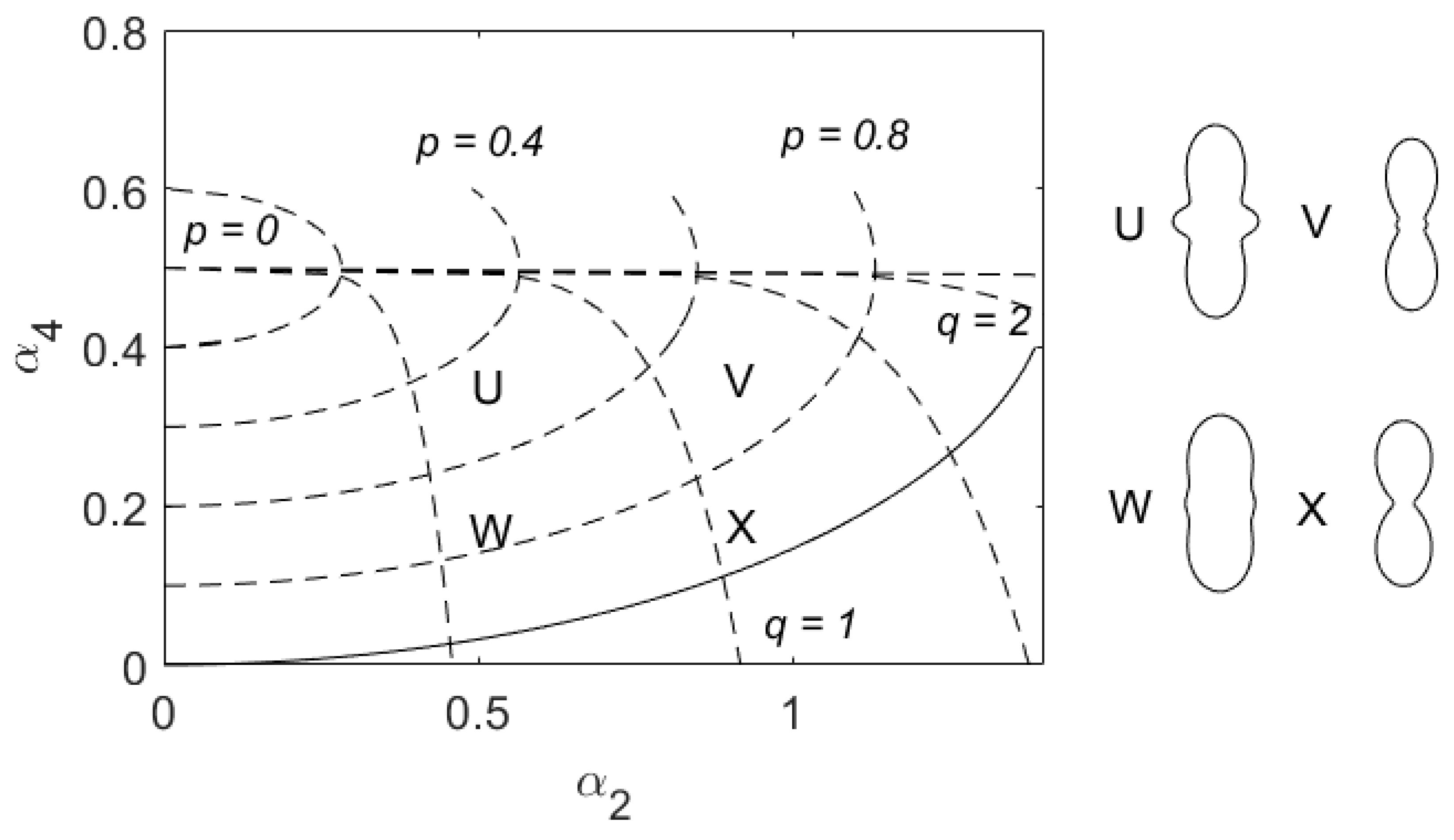
When a target passes through the vertical-pointing beam, the radar records the logarithmically transformed intensity of the echo signal arising from backscattering by the target. The modulation of the intensity of the radar signal is post-processed to find the target’s direction and speed of movement, the (axial) direction to which it is aligned [25,26] and information about the target’s character that provides information about its identity: RCS a₀, shape parameters α₂ and α₄ and wingbeat frequency f_w. The range of a₀ values retrieved varies over 3 orders of magnitude and it is common practice in radar work to work with the logarithmically transformed value, expressed in decibel units (dBsc—decibels relative to 1 cm², is used in our study). However, the mass versus RCS relationship for insects shows considerable spread (the uncertainty of mass range calculated based on value of a₀ is approximately ±40% [27]) and in this work the directly measured RCS parameter a₀ is therefore used, rather than mass, as a discriminating quantity. The polarization pattern parameters are confined by radar scattering theory to the ranges, 0 ≤ α₂ ≤ $\sqrt{2}$ and 0 ≤ α₄ ≤ 1 [23]. Non-zero values of α₂ occur when the polarization pattern is elongated in the direction of the insect’s body axis, as is typically the case for most insects (see examples in Figure 1). The parameter α₄ adds a four-lobed component and if sufficiently large it produces two additional lobes in the polarization pattern, at right angles to the elongation direction. (For very large insects, these lateral lobes can become larger than those along the body axis [23] but this does not arise with the species occurring at Bourke and thus is not considered further in this study.) The IMR identifies wingbeat frequencies f_w in the range 21 to 150 Hz [8]. The dataset considered here comprises only those targets for which a good-quality fit to the observed echo signal was obtained and all four of the target-character parameters were retrieved. As in the earlier 4D peak-finding work, the orthogonal shape variables p and q will be employed in preference to α₂ and α₄ to define boundaries in this study (Figure 1); they are obtained via Equations (A1) and (A2) [24]. However, we also use α₂ and α₄ for general analysis.

2.2. Weather

Temperatures for our study were derived from the meteorological component of The Air Pollution Model (TAPM) [28], which draws on operational meteorological observations to estimate winds and temperatures throughout the atmospheric boundary layer at a fine scale. TAPM is optimized for high-resolution weather simulation and has been tested in a wide range of locations, both in Australia and overseas [29,30]. In previous work [5], the model has been verified by comparing the simulated surface winds, air temperatures and specific humidities from the model with observations from the Australian Bureau of Meteorology automatic weather station (AWS) at Bourke (very close to the radar site): the TAPM root mean square (rms) of the hourly averaged surface wind speeds and temperatures are 1.2 m s⁻¹ and 7.6 °C, which are close to the rms averages of AWS observations (1.8 m s⁻¹, 7.6 °C) [22]. We therefore conclude that TAPM air temperatures are sufficiently accurate to use in this study as estimates of the temperature experienced by each observed target at its flying height.

3. Results

3.1. Clustering Analysis

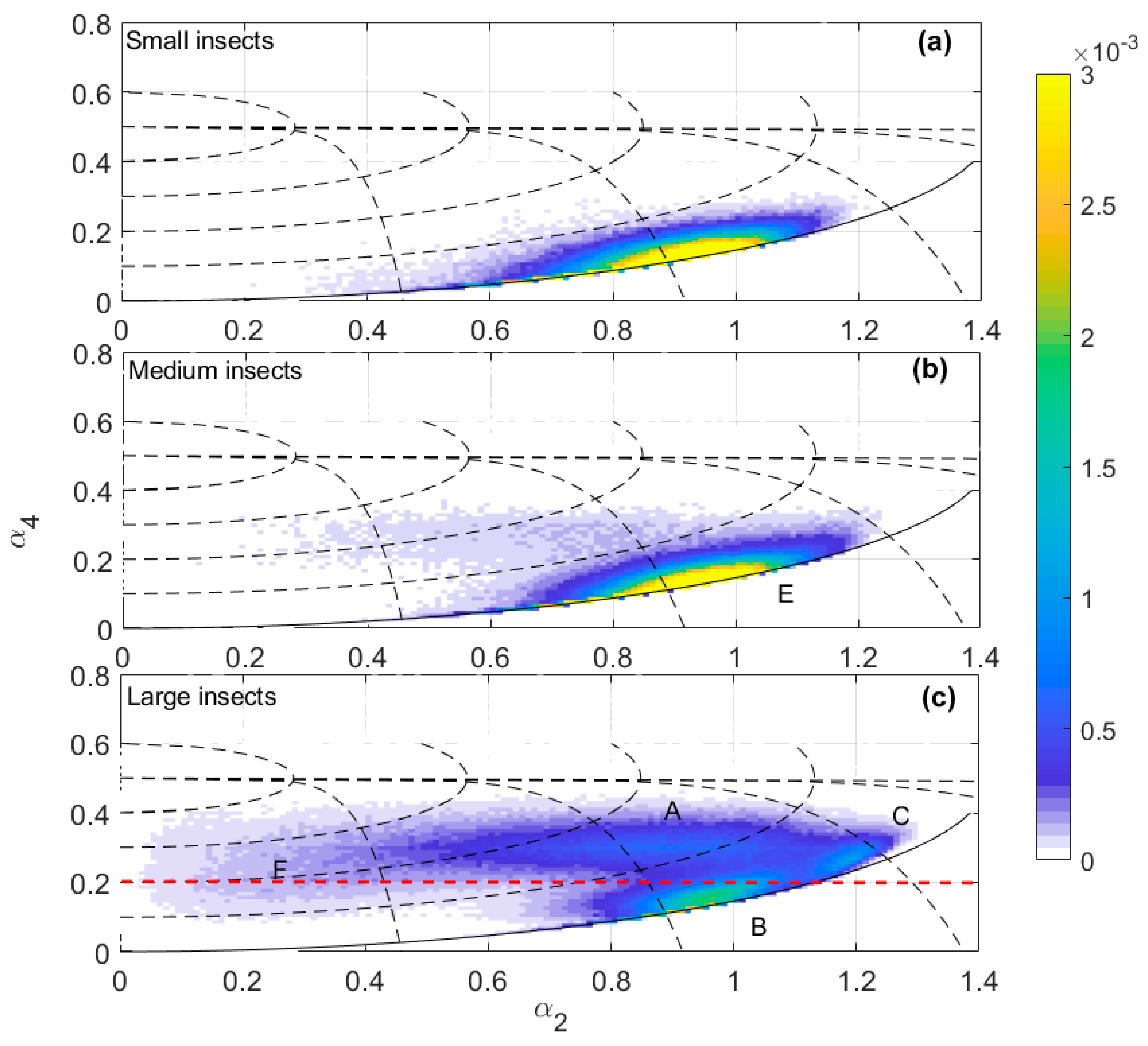
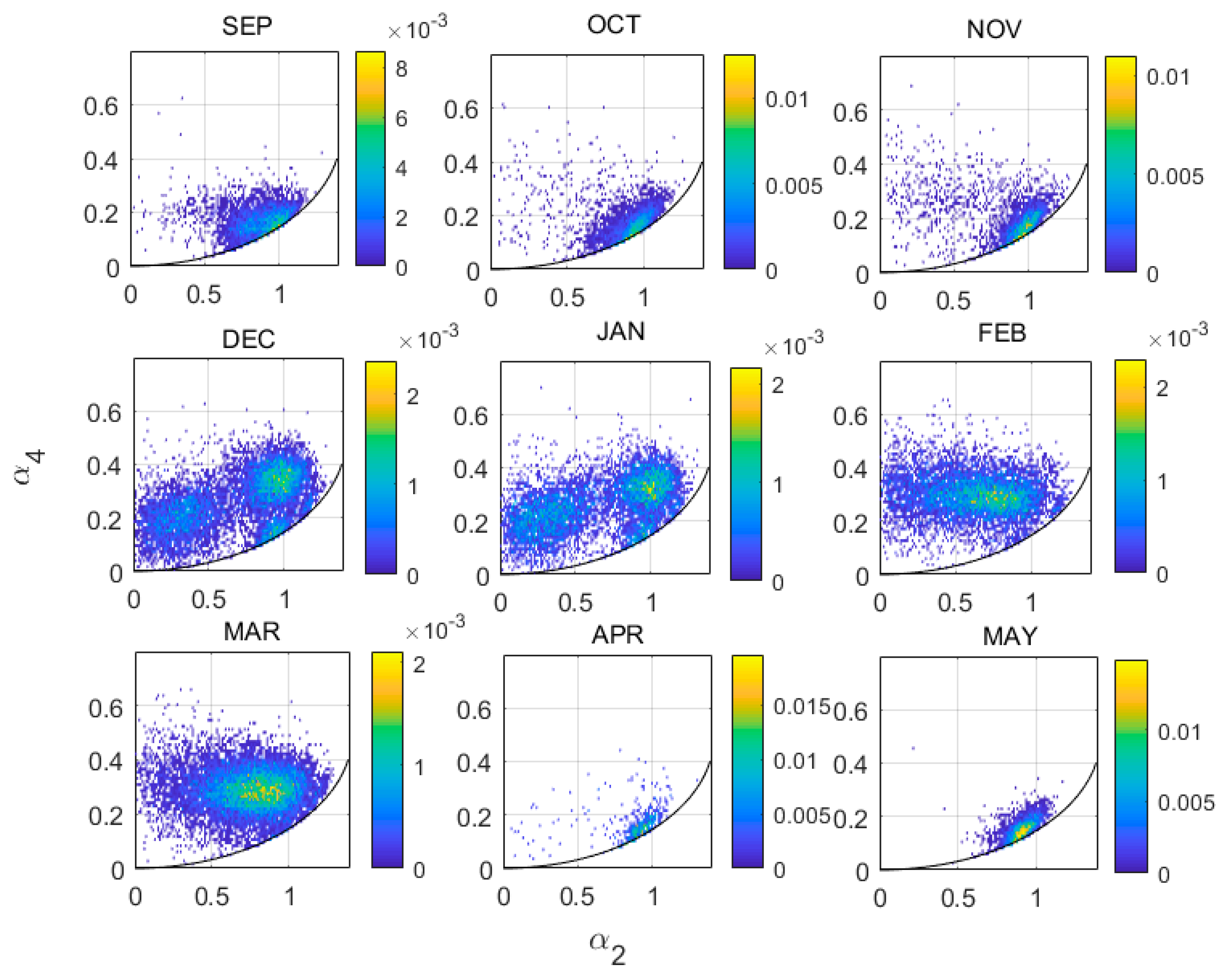
Partitioning the 14-year target sample by a₀ into three subsets, we can easily identify clusters of targets on the (α₂, α₄) plane (Figure 2). (In this paper we use ‘cluster’ to refer to a concentration of data points on the (α₂, α₄) plane, ‘region’ to refer to the part of the plane occupied by a cluster and ‘class’ to refer to the subsample selected based on the criteria introduced below.) ‘Small insects’ (−23 dBsc < a₀ < −13 dBsc) and ‘medium insects’ (−13 dBsc < a₀ < −3 dBsc) (Figure 2a,b) form a single cluster elongated in the α₂ direction, approximately in the location of the ‘main cluster region’ (MCR) previously identified [27]. Therefore, the shape parameters do not discriminate different clusters for targets of these sizes. In contrast, there are three major clusters in the ‘large insects’ subset (−3 dBsc < a₀ < 7 dBsc) (Figure 2c). These three clusters, denoted A, B and C, occurred at the same locations in the (α₂, α₄) plane across years and seasons. In 2005–2006, for example (Figure 3), cluster A was present from December to March. However, it showed some variation, being more concentrated with 0.6 ≤ α₂ < 1.1 during December and January but extending to smaller α₂ values, nearly reaching α₂ = 0, during February and March and almost splitting into two (clusters A and F, discussed further below). This variation was seen occasionally in other years and was noted in the previous 4D peak-finding investigation where the low-α₂ cluster was denoted LL6₅ and the high-α₂ one LL8₁₀ [24]; however, it is not consistent enough to appear in the plot for all years. Cluster B was dominant from September to November, less clear from December to March and then dominant again in April and May. Cluster C can be barely seen except in February when a small sample appeared. Both B and C were partially included as LL10₁₃ in the previous investigation [24]. The weak cluster at the position of cluster A in medium insects (Figure 2b) is possibly a remnant of cluster A as the cut between large and medium insects is quite artificial (discussed below); it may also have arisen as an artefact of the electronic gating system used for data acquisition [4]. The coordinates p and q (see Figure 1) shown in Figure 2 follow the forms of all three clusters and are thus well suited to defining their ranges.

In order to classify each cluster for the large-size insects across years, each cluster is defined in the p-q coordinates, firstly based on knowledge of their previous definitions [24] and the visualization of their p and q range demonstrated here, followed by a second classification step based on their size and wingbeat distributions. Cluster A corresponds to a single class, LL8₁₀, of the previous study [24], in which clusters B and C were both included in a single class, ML/MM, with an a₀ peak in the medium-size range but which extended into the large-size range. Here their definitions are slightly modified. Based on p and q ranges, a broad range of a₀ (−5 dBsc < a₀ < 7 dBsc) and wingbeat frequency (21–50 Hz), it can be seen that clusters A and C have normal a₀ distributions in log-space (i.e., with a₀ expressed in dBsc; Figure 4a,c). This simple distribution suggests they each comprise a single dominant species and it provides some support for the validity of the cluster approach. The f_w distribution is approximately normally distributed for cluster A (Figure 4f) but not C (Figure 4h), where it is cut off at the 21-Hz lower limit of our observations. Wingbeat frequencies are predominantly smaller than 30 Hz for this cluster. The a₀ and wingbeat definitions for each class (

Table 2. Class boundaries for large insects and calculated mass range ¹ based on the size distribution.

	a0 (in dBsc)	p	q	fw (Hz)	Mass Range (mg) 2
Class A	−3.3, 6.7	0.58, 0.83	0.73, 1.28	22.6, 35	143–395
Classes B and D 3	−3.6, 4.9	0.88, 1	0.82, 1.25	21, 29	105–245 119–282
Class C	−3.3, 4	0.9, 1	1.27, 1.6	21, 28.2	121–258

¹ In the traditional classes we used before, large insects are in the range of approximately ~100–1000 mg, medium insects ~30–100 mg and small insects smaller than 30 mg. ² From the mean ± 1 std of the normal distribution of a₀ in Figure 4. ³ D is selected with the extra criteria that the peak of a₀ > −3 dBsc and f_w < 27 Hz.

) are derived from the a₀ and f_w distributions, with consideration of their closeness to other clusters to minimize cross-contamination while maintaining sample size and differ slightly from those in Reference [24]. This step also involved minor fine tuning of the p and q limits.

Cluster B, in contrast, overlaps with the medium and small insect targets in the (α₂, α₄) plane. Figure 4b shows that its a₀ (dBsc) distribution is not normal, indicating that it is continuous with that of medium moths. The size distribution of medium moths (cluster E, Figure 2b) is also truncated (Figure 4e), suggesting that the size categories are imposing an artificial partitioning; this is consistent with the previous study [24] which combined these into a single class (ML/MM). However, on some nights the a₀ distribution did peak in the large-size range. Therefore, an additional selection criterion was introduced to obtain a sample without insects that were probably just large examples of a medium-size type. To do this, we examined individual nights and selected those for which the size and wingbeat distribution had a peak a₀ > −3 dBsc and f_w < 27 Hz. We will treat the cluster-B samples from these nights as a subclass that we will refer to as D. The sample size of D is only about one tenth that of cluster B (which includes D). Cluster D has a normal a₀ (dBsc) distribution and a narrower distribution of f_w compared to cluster B, with a peak at 24 Hz (Figure 4d,i). The f_w values of cluster B (Figure 4g) and those of medium insects (cluster E, Figure 4j) are similarly distributed across the entire range (21 to 50 Hz) and both peak at ~27 Hz, which is consistent with the majority of cluster B being a continuation of the medium size cluster. The final definitions of these clusters are listed in Table 2 and illustrated in Figure 7 and Figure A1.

3.2. Flight Temperature

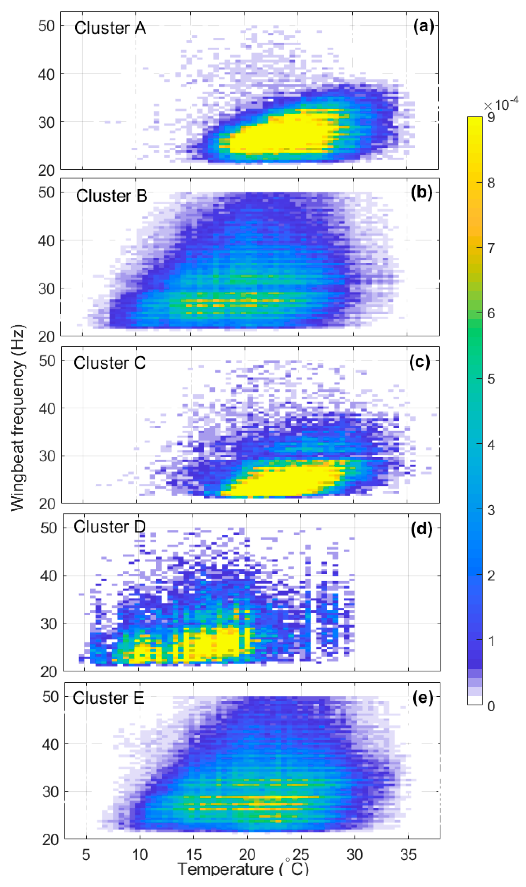
We can understand more about insect flight capabilities during migration by studying how wingbeat frequency varies with air temperature for each cluster (Figure 5). In general, the greatest difference between clusters is the range of temperatures T at which insects fly. Insects within cluster A and C require warmer conditions (T > ~15 °C), while insects within clusters B, D and E flew when temperatures were lower, down to ~8 °C for, 6 °C for B and 4 °C for D (

Table 3. Means and standard deviations of wingbeat frequency (f_w) and air temperature (T) for each cluster and coefficient of linear regression of the f_w on T for each cluster.

	Cluster A	Cluster B	Cluster C	Cluster D	Cluster E
fw (mean ± std) 1	27.9 ± 3.7	31.5 ± 6.7	26.1 ± 4.4	27.7 ± 4.8	31.7 ± 6.6
T (mean ± std) 2	24.2 ± 3.8	19.8 ± 5.5	23.9 ± 3.7	16.0 ± 4.7	21.2 ± 5.4
coefficient estimate	1.134 ± 0.001	1.496 ± 0.002	1.076 ± 0.002	1.610 ± 0.015	1.413 ± 0.002

^1,2 All samples test as significantly different (two sample t-test, P < 0.05) from other clusters in terms of means and standard deviations of f_w and T.

). Clusters B and E also have similar temperature and wingbeat-frequency distributions, which is again consistent with each of them really being a single broad cluster; the slightly lower temperature range of B may be due to its inclusion of D, which exhibits the coolest conditions. All clusters show a trend of increasing wingbeat frequency with temperature, with clusters A and C showing only a modest increase and clusters B, D and E a stronger one (Table 3).

3.3. Year-to-Year and Seasonal Variations

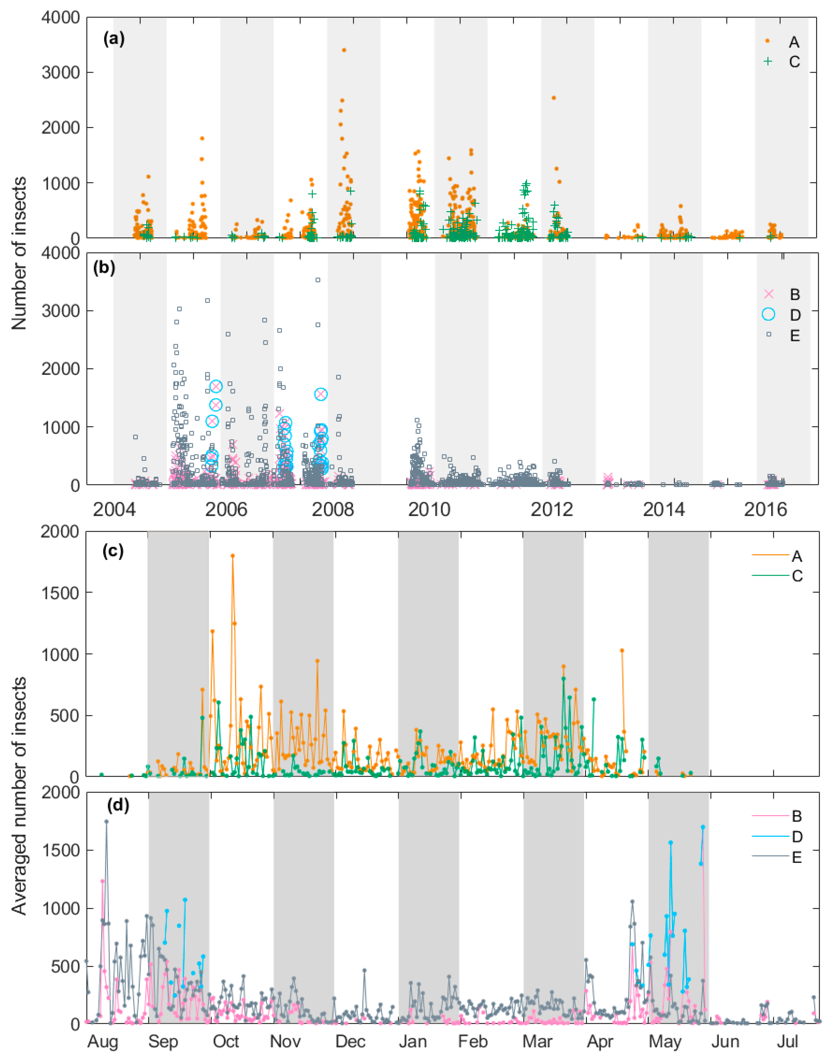
Another feature that may help us to determine the identity of each class is their varying incidence and intensity across both years and seasons (Figure 6). The three large-target classes showed considerable differences in these respects. Class A was present in all years, with numbers particularly high in 2008–2009 and 2010–2011. It is present throughout the insect flight season (September–May) but is most common in late spring (October–November) and to a lesser extent autumn (March–April). Class C was recorded in most years but less frequently than class A, except in 2011–2012: the peak year for class C and one of the weakest for class A. Class C shows spring and autumn peaks like those of class A, though a little earlier in spring (October but not November) and relatively stronger in autumn. The lower numbers of insects since 2013 is partly due to the known drop in radar performance but probably also to reduced insect populations because of drought. These years have been omitted from the analysis of within-season variation (Figure 6c,d).

Moths of class B, as well as medium-sized moths (class E), were most numerous from 2005–2008, that is, in years when moths from class C and to a lesser extent class A, were less numerous (with the exception of 2008). Class B moths were common during early spring (August, September) and late autumn (late April and May) but were conspicuously low in summer (December, January). Medium moths showed a generally similar pattern except that they did not persist into May. Moths within class D were recorded only in September and May and only in 2006–2008 (Figure 6b).

4. Identity of Species Forming the Target Classes

4.1. Available Resources that Could Help with Identification of Classes

In order to determine the insect species that comprise each target class, we will draw on ancillary data of three types. These will allow us, first to identify proxy species with measured RCSs and CLPPs and use these to infer mass values for the IMR-observed targets, then relate these masses to those of morphologically similar Australian species and finally compare these with Australian migrant species known to be present in the region where the radar observations were made.

4.1.1. RCS and CLPP Data of Proxy Species

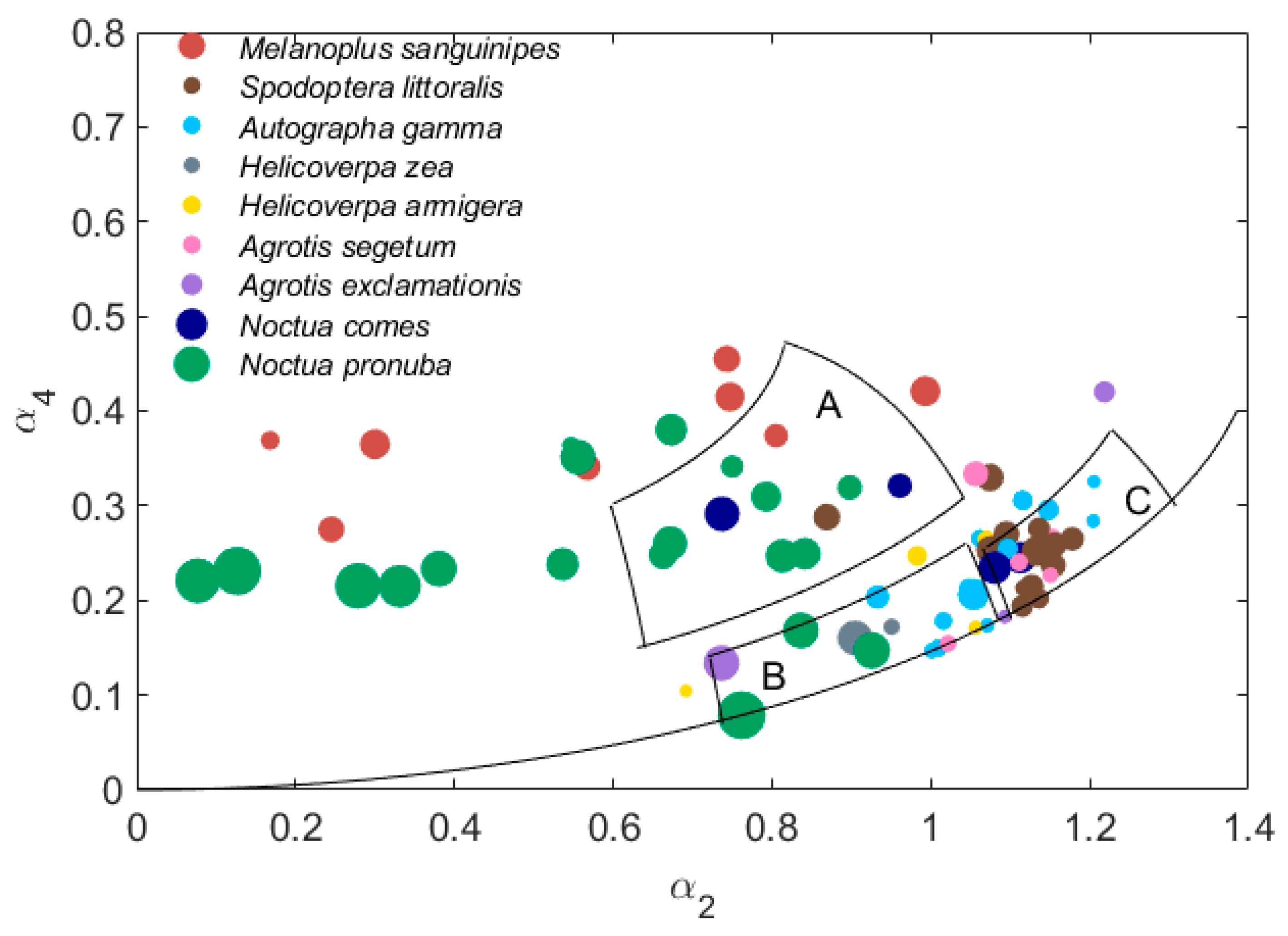
The location on the (α₂, α₄) plane of some specimens of similar-sized but non-Australian species [27] could help identify insect species in the radar observations (Figure 7). The large size range insects in region A are mainly moths: N. pronuba (N = 20), the Lesser Yellow Underwing Noctua comes (N = 4) and the Migratory Grasshopper Melanoplus sanguinipes (N = 8). The large-size insects in region B are all noctuid moths, mainly Helicoverpa zea (N = 2) and Agrotis exclamationis (N = 3). Three N. pronuba also fall within this region. Large-size insects found in region C are mostly A. gamma (N = 13), Agrotis segetum (N = 5) and the African Cotton Leafworm Spodoptera littoralis (N = 13).

N. pronuba, N. comes and M. sanguinipes form a horizontal band on the (α₂, α₄) plane, which is similar in form to cluster A (though it extends to smaller α₂), though some specimens of N. pronuba fall into region B. Points for other noctuid moths spread throughout the plane, covering both the B and C regions, which is known as the main cluster region (or MCR). There is a clump of noctuid moth individuals close to the location of region C. However, they are concentrated in the lower part of this region. All the data points on the plane suggest that there are overlaps between different species but it should be remembered that these points are for individual specimens and there is large variability in both α₂ and α₄ between individuals of a given species.

4.1.2. Aerial-Netting and Light-Trap Catches

Light-trap catches in northern NSW at Point Lookout, Mt. Dowe (which is 405 km east of Bourke) [18,31] and Stanley, Tasmania [32], as well as aerial netting at Trangie [17], revealed common noctuid species (

Table 4. The mass range ¹ (mg) and estimated a₀ values (in dBsc) for candidate Australian insect species together with the percentage of total catch for each species caught in light traps at Point Lookout (30°29′S, 152°28′E) and Mt. Dowe (30°17′S, 150°10′E) NSW from 1985 to 1989 [18,31] and from aerial catches at Trangie, NSW (31°59′S, 147°57′E) in late September [17] and at Stanley, Tasmania (40°46′S, 145°17′E) during late September and early October 1973 [32].

	Min (mg)	Max (mg)	Mean (mg)	Range 2 (mg)	a0 (dBsc)	Point Lookout	Mt Dowe	Trangie	Stanley
Austracris guttulosa (N = 20)	728	2391	1375	880–1869	4.7–8.1
Chortoicetes terminifera (N = 24)	244	860	415	241–589	0.5–4.2
Agrotis infusa (N = 54)	163	382	231	189–273	(−0.6)–1.1	20.4%	94.3%	10%	~10%
Agrotis munda (N = 3)	124	183	146	-	(−2.9)–(−0.8)	1.8%	0.8%	15%	~40%
Helicoverpa armigera (N = 4)	90	197	141	-	(−5.1)–(−4.1)	4.4%	0.1%
Mythimna convecta	wingspan is about 40 mm while A. infusa has an average of 47mm					18.5%	0.4%
Helicoverpa punctigera (N = 22)	40	152	106	77–133	(−6.4)–(−2.5)	6.1%	1.5%

¹ Data derive from an unpublished dataset collated by V.A.D. and originate from various field studies undertaken in eastern Australia. All measurements are thought to be of freshly dead specimens, so they should be representative of insects undertaking migration. ² Mean ± 1 s.d.

). A. infusa made up 20.4% of the catch at Point Lookout but dominated it at Mt. Dowe with 94.3%. It was also a prominent species at the other two sites, constituting ~10% of the catch. The Common Armyworm Mythimna convecta was almost as common as A. infusa at Point Lookout but relatively rare at Mt. Dowe. In Victoria, M. convecta is regularly caught in light traps in spring and these catches proved to have come from a distant population [33]. However, this species was not recorded at Trangie or Stanley. Of the remaining noctuids, H. punctigera and Agrotis munda were prominent at both sites, while H. armigera was only recorded at Point Lookout but not at Mt. Dowe. A. munda was the dominant species at Stanley and Trangie and in South Australia (mentioned in Reference [32]).

4.1.3. Australian Morphological Data

Masses for several of the Australian candidate species are provided in Table 4. Measurements of body mass for M. convecta were not available from any recent studies so it has been inferred from that of other noctuids with similar wingspans. Radar cross-sections a₀ of these species, estimated from their mean mass [9], are also given in Table 4. Based on estimated a₀ values Table 4 and insect categories used in Section 3.1, these species can be assigned to medium and large size groups and this enables us to match them with our classes later. A. guttulosa, C. terminifera and A. infusa are categorized as large insects based on their mass range and estimated large a₀. H. punctigera have an average a₀ close to −2.5 dBsc [27], which categorizes them as medium-to-large moths. M. convecta has a wingspan (~40 mm) similar as that of A. gamma (~41 mm, N = 3, a₀ = −2.6 dBsc). Thus, it can be inferred that M. convecta is about the same size as A. gamma which is categorized as medium-to-large. H. armigera (a₀ = −0.66 dBsc) and A. munda (a₀ = −0.5 dBsc) are close to the boundary between medium and large moths and could fall into either category.

4.2. Identity of Species Forming the Target Classes

Class A has been associated with the C. terminifera in previous studies [7,8]. This is supported here by (1) the frequency and large size of class-A events in 2008–2011, when high numbers of this species were reported by the APLC in their monthly locust bulletin [19] and (for 2010–2011) in previous studies [34,35], (2) the shorter (October–April) seasonal pattern with some activity continuing through the summer and (3) the higher temperatures at which class A insects fly. The previous radar-target-class selection criteria (Table A2) distinguish C. terminifera and large moths only on whether α₄ was greater or smaller than 0.2. While this selected cluster A quite well, it very likely led to the inclusion of large-moth data from the higher-α₂ part of the MCR. The new criteria for defining class A avoid this ambiguity and thus reduce contamination of the locust dataset. The non-native RCS and CLPP data show that moths (e.g., N. pronuba) can be present in region A but moth species of this size are not known as migrants in Australia.

In some months, this extension entirely separates to form a distinct cluster F at lower α₂ and α₄ values (Figure 3, December and January), although a split was also recognized in our previous 4D peak-finding study [24], which analyzed individual nights. It is possible that cluster F is due to the spur-throated locust A. guttulosa, which is only active during summer in the Bourke region and only in some years. For example, nocturnal migrations of A. guttulosa as well as C. terminifera were recorded on 29 October 2010 by the IMR at Bourke in the APLC bulletin [19] and later reported in Melbourne on 12 Nov [34]. Our data confirm that cluster F appeared during these times, alongside cluster A. A. guttulosa has a generally similar morphology to C. terminifera but is larger (Table 4). The size distributions during these nights showed an a₀ peak at ~3 dBsc but there is a tail to beyond 5 dBsc. Further examination of these relatively infrequent events is beyond the scope of the present investigation.

Class C is located in a region of the (α₂, α₄) plane that laboratory measurements indicate is dominated by moths [24]. However, the temperatures at which these targets were flying (Figure 5) as well as their seasonal patterns (Figure 6c) are similar to those from class A, so it appears more likely that they are orthopterans of some type or perhaps some other cold-intolerant order. It is unlikely that insects in class C are a form of C. terminifera, as in some months they were present when there was no class A. The year-to-year pattern of appearances also differs between the two classes, especially in 2011–2012 when insects from class C are the more numerous. The only other orthopteran to be caught in the aerial net at Trangie was a single specimen of the slightly smaller acridid grasshopper, Aiolopus thalassinus [36]. This is certainly large enough to produce a detectable radar echo but with a size range overlapping that of C. terminifera and a similar morphological form, it seems unlikely that it would form a distinct class. Thus, class C cannot be attributed to any species or insect taxon at this stage.

Both class B and the medium-sized insects (E) in the MCR can be identified as moths. They show very similar temperature ranges for flight and this range is much lower than that for classes A and C (Figure 5). The moths in class B will be larger species and larger specimens of “medium-sized” species that overlap our arbitrary boundary between medium and large. With regards to medium-size moths, H. punctigera and Athetis tenuis appear to be dominant candidates. H. punctigera is one of the most common nocturnal insects moving above the boundary layer [17,32]. Case studies have shown that H. punctigera populations migrated southward on pre-frontal winds from the inland into cropping areas of northern NSW, southern QLD and western VIC in the early spring of 1983 and during 1989–1991 [37,38]. In autumn, return migrations have been rarely reported but they presumably occur as in winter H. punctigera is almost exclusively confined to the far inland. A. tenuis was one of the most numerous species in the aerial netting catches at Trangie, NSW. No mass is available but its wingspan of ~25 mm suggests it falls into our medium category. H. armigera is considered less migratory and constituted only a modest proportion of the light trap catches at Point Lookout and Mt. Dowe (Table 4), so there is little reason to include it. The smaller moths Heliothis punctifera and two pyralid species, Loxostege affinitalis and Nomophila australica, were also caught in the aerial net at Trangie and may be included in our medium (H. punctifera) and small (the pyralids) size classes.

Class D is a subset of B, comprising large targets distinguished also by a low peak in the wingbeat-frequency distribution. Their flight-temperature range was generally similar to that for other classes (B and E) attributed to moths but shifted lower by 3–5 °C (Figure 5). They were observed only in September and May. These features are all compatible with the species A. infusa, which is known to be active at low temperatures (E.W., unpublished observations). Bourke is somewhat to the west and north of areas where A. infusa is believed to breed [39]; however, A. infusa were light-trapped at Wilcannia, ~300 km southwest of Bourke, in October 2016 (E.W., unpublished observation), which indicates the species is present in spring in this region and possibly breeds there. But the years class D were observed do not correspond to years of high A. infusa numbers in the mountains (1998, 2001, 2005 and 2010) [40], so this identification is very tentative. Other larger moths that are candidates for class D are the noctuids A. munda and M. convecta. A. munda was abundant in the light trap catches at Trangie [17] and Stanley [32] and in South Australia (mentioned in Reference [32]). Back-tracking from the light-trap sites in northern NSW [18,31] suggested they originate from western NSW or Queensland. However, there is little information on detailed migration patterns of this species as their populations are rarely monitored. M. convecta has long been known as a pest of cereals throughout temperate and subtropical Australia [41]. In one study, its probable source areas were identified as the extensive grasslands of south-west and central Queensland and the adult peak season was spring (September–November) in northwest NSW, the region where Bourke is located [33].

5. Discussion

The method and findings presented in this paper provide a firmer basis for recognizing classes of targets in ZLC-radar datasets. The criteria previously used for observations in inland eastern Australia have been refined and two new classes recognized. This improves the precision with which observations at Bourke and other sites in this broad region, can be interpreted. The likelihood of different taxa being combined into the same class is reduced, with consequent benefits for researchers or pest managers seeking to make use of the data.

The classes presented in this paper differ slightly from those identified in the earlier 4D peak finding study [24], in which seven classes were recognized: one comprising small insects, three comprising medium-size insects and three comprising large insects. Small insects constitute a single class in both studies. The earlier study employed two different methods and one of these recognized three classes of medium sized insects, distinguished by their wingbeat frequencies; the second method and the present study, merged two of these into a single class with a wide wingbeat frequency range. The third medium-size class recognized in the earlier study, MvHM, had very high wingbeat frequencies (around 75 Hz) and was detected on only a few nights. This class was not apparent in the more aggregated samples used in this study. With regards to the large-size insects, class A is common to both studies while in the previous study class B was regarded as part of the medium-size class E; which is consistent with the finding here that the medium/large division between classes B and E, at −3 dBsc, is essentially arbitrary. Class LL10₁₃ of the previous study is intermediate between our classes B and C; it was detected by only one of the two methods investigated there and only infrequently. Class C was recorded only a few times in 2005–2006, the flight season analyzed in the earlier work, but quite frequently in some other years; we will regard it as ‘new’ to this study and consider LL10₁₃ as not confirmed. The second new class has been defined from class D, which has a larger size and lower wingbeat frequency range than B and appears to be slightly more cold-tolerant. It occurred only infrequently and hardly at all in 2005–2006.

In our study, the large-insect classes A and C were well separated from the rest of the dataset. However, class B, which is located in the MCR, has no natural break in the size (a₀) distribution to separate it from the medium-insect class E. Measured α₂ and α₄ values for the non-Australian moth species often also fell into this region, for all but the largest specimens. Several Australian migrant moth species have masses similar to those of the measured species with (α₂, α₄) in the MCR and sizes near the border between our medium and large size categories. Some migrations of medium-sized or class D large insects involved massive numbers of individuals, so are likely to be important ecologically. It will be difficult to determine whether they are dominated by one species or consist of a mixture.

The methodology proposed in this paper helps to discern and identify classes of insect targets in a long-term radar observation dataset. Nevertheless, some classes appear to comprise a number of species with similar morphologies (as seen by 3-cm wavelength radio waves). Such mixed classes may include species that occur in large numbers only infrequently, which adds to the difficulty of making confident identifications. Parallel long-term trapping and survey programs provide strong support for associating species to classes, at least in particular years but in inland Australia these are available only for the C. terminifera. This study shows that air temperatures at the height of the targets provide useful indications of the target identities, at least at the population level. Temperatures can be estimated from operational meteorological models (or better, their regional-scale derivatives), so this factor can potentially be included in the observation-interpretation process in a routine way, perhaps even within the time constraints of pest-management decision-makers.

There may be some scope for increasing the precision with which classes can be discerned. For example, in the earlier study of a single year of observations, a method based on multiple 2-D clusters found more classes than the 4D version; however, only the latter could be automated and made fully objective [24]. Measurements of the RCSs and CLPPs of Australian species might appear to provide better information on which to base associations of species and classes but when morphologically-close proxy species are available, as in this study, it is not clear that much would be gained. However, measurements of larger samples of each species, to capture the full range of a₀ and shape-parameter values that migrant individuals can attain, would be valuable. All RCS measurements should be accompanied by measurements of mass (of live or freshly dead individuals) and body dimensions, as this provides a means of relating the laboratory measurements to field populations. Useful RCS and CLPP information may also be obtainable via electromagnetic modelling [42], though with reduced strength of inference if used for target identification. Knowledge of the temperature-range for sustained flight for each species of interest will also have interpretive value and may be obtained through careful laboratory measurement [43] or inferred from field observations.

6. Conclusions

The target classes identified as predominant in the previous study of a single flight season occurred frequently in the 14-year dataset, though with some variation of proportions and occurrence from year to year. Additionally, two new classes were recognized. Medium-sized insects are largely confined to a single area of the (α₂, α₄) plane, the ‘main cluster region’ (MCR) but large insects show a wide variety of shape-parameter values. The air temperatures at the height of the targets, derived from meteorological models, have been found to be a valuable additional indicator of target identity. By drawing on knowledge of the migrant species found in the broad geographical region around the radar site, together with morphological measurements and radar cross-section data for proxy species, we have made tentative identifications of the insect taxa likely to be attributed to each class. The large-insect class A is attributed to the C. terminifera and our revised criteria will reduce contamination of the locust datasets. Based on the warmer temperatures at which they are flying and the seasonal pattern, class C may be a smaller orthopteran; however, at this stage not even a tentative attribution can be made. Both class B and the medium-sized cluster in the MCR (class E) can be identified as moths but not one or more specific species. Class D may be the A. infusa, as it comprises large targets that fly in low temperatures in early spring and late autumn with a low wingbeat frequency. However, some other species, such as A. munda and M. convecta, cannot be excluded from this class at this stage. Finally, we note that measurements of the RCSs and CLPPs of Australian species would avoid the need to rely on proxies and thus provide firmer information on which to base associations of species and classes in the future.

References

- Drake, V.A.; Reynolds, D.R. Radar Entomology: Observing Insect Flight and Migration; CABI: New York, NY, USA, 2012. [Google Scholar]
- Chapman, J.W.; Drake, V.A.; Reynolds, D.R. Recent insights from radar studies of insect flight. Annu. Rev. Entomol. 2011, 56, 337–356. [Google Scholar] [CrossRef] [PubMed] [Green Version]
- Drake, V.A.; Wang, H.K.; Harman, I.T. Insect monitoring radar: Remote and network operation. Comput. Electron. Agric. 2002, 35, 77–94. [Google Scholar] [CrossRef]
- Drake, V.A.; Hatty, S.; Symons, C.; Wang, H. Insect Monitoring Radar: Maximizing Performance and Utility. Remote Sens. 2020, 12, 596. [Google Scholar] [CrossRef] [Green Version]
- Hao, Z.H.; Drake, V.A.; Sidhu, L.; Taylor, J.R. Locust displacing winds in eastern Australia reassessed with observations from an insect monitoring radar. Int. J. Biometeorol. 2017, 61, 2073–2084. [Google Scholar] [CrossRef]
- Otuka, A.; Matsumura, M.; Tokuda, M. Development of method to forecast soybean leaf damage by common cutworm using entomological radar and searchlight trap. J. Eng. 2019, 2019, 7531–7533. [Google Scholar] [CrossRef]
- Wang, H.K. Evaluation of Insect Monitoring Radar Technology for Monitoring Locust Migrations in Inland Eastern Australia. Ph.D. Thesis, The University of New South Wales, Canberra, Australia, 2008. [Google Scholar]
- Drake, V.A.; Wang, H.K. Recognition and characterization of migratory movements of Australian plague locusts, Chortoicetes terminifera, with an insect monitoring radar. J. Appl. Remote Sens. 2013, 7, 1–17. [Google Scholar] [CrossRef] [Green Version]
- Chapman, J.W.; Smith, A.D.; Woiwod, I.P.; Reynolds, D.R.; Riley, J.R. Development of vertical-looking radar technology for monitoring insect migration. Comput. Electron. Agric. 2002, 35, 95–110. [Google Scholar] [CrossRef]
- Smith, A.D.; Riley, J.R.; Gregory, R.D. A method for routine monitoring of the aerial migration of insects by using a vertical-looking radar. Philos. Trans. R. Soc. B 1993, 340, 393–404. [Google Scholar] [CrossRef]
- Wang, H.K.; Drake, V.A. Insect monitoring radar: Retrieval of wingbeat information from conical-scan observation data. Comput. Electron. Agric. 2004, 43, 209–222. [Google Scholar] [CrossRef]
- Chapman, J.W.; Reynolds, D.R.; Brooks, S.J.; Smith, A.D.; Woiwod, I.P. Seasonal variation in the migration strategies of the green lacewing Chrysoperla carnea species complex. Ecol. Entomol. 2006, 31, 378–388. [Google Scholar] [CrossRef]
- Jeffries, D.L.; Chapman, J.W.; Roy, H.E.; Humphries, S.; Harrington, R.; Brown, P.M.; Handley, L.J. Characteristics and drivers of high-altitude ladybird flight: Insights from vertical-looking entomological radar. PLoS ONE 2013, 8, e82278. [Google Scholar] [CrossRef] [PubMed] [Green Version]
- Wotton, K.R.; Gao, B.; Menz, M.H.M.; Morris, R.K.A.; Ball, S.G.; Lim, K.S.; Reynolds, D.R.; Hu, G.; Chapman, J.W. Mass seasonal migrations of hoverflies provide extensive pollination and crop protection services. Curr. Biol. 2019, 29, 2167–2173. [Google Scholar] [CrossRef] [PubMed]
- Chapman, J.W.; Nesbit, R.L.; Burgin, L.E.; Reynolds, D.R.; Smith, A.D.; Middleton, D.R.; Hill, J.K. Flight orientation behaviors promote optimal migration trajectories in high-flying insects. Science 2010, 327, 682–685. [Google Scholar] [CrossRef] [PubMed]
- Riley, J.R.; Reynolds, D.R. Radar-based studies of the migratory flight of grasshoppers in the middle Niger area of Mali. Proc. R. Soc. Lond. B Biol. Sci. 1979, 204, 67–82. [Google Scholar]
- Drake, V.A.; Farrow, R.A. A radar and aerial-trapping study of an early spring migration of moths (Lepidoptera) in inland New South Wales. Aust. J. Ecol. 1985, 10, 223. [Google Scholar] [CrossRef]
- Gregg, P.C.; Fitt, G.P.; Coombs, M.; Henderson, G.S. Migrating moths collected in tower-mounted light traps in northern New South Wales, Australia: Influence of local and synoptic weather. Bull. Entomol. Res. 1994, 84, 17–30. [Google Scholar] [CrossRef]
- Locust Bulletin, Australian Plague Locust Commission, Australia. Available online: https://www.agriculture.gov.au/pests-diseases-weeds/locusts/bulletins (accessed on 15 October 2019).
- Gregg, P. Pollen as a marker for migration of Helicoverpa armigera and H. punctigera (Lepidoptera: Noctuidae) from western Queensland. Aust. J. Ecol. 1993, 18, 209–219. [Google Scholar] [CrossRef]
- Warrant, E.; Frost, B.; Green, K.; Mouritsen, H.; Dreyer, D.; Adden, A.; Brauburger, K.; Heinze, S. The Australian Bogong moth Agrotis infusa: A long-distance nocturnal navigator. Front. Behav. Neurosci. 2016, 10, 77. [Google Scholar] [CrossRef] [Green Version]
- Hao, Z.H. Testing Ideas about Australian Insect Migration Using Entomological Radar Observations and a Regional Scale Meteorological Model. Ph.D. Thesis, University of New South Wales, Canberra, Australia, 2016. [Google Scholar]
- Dean, T.J.; Drake, V.A. Monitoring insect migration with radar: The ventral-aspect polarization pattern and its potential for target identification. Int. J. Remote Sens. 2005, 26, 3957–3974. [Google Scholar] [CrossRef]
- Drake, V.A. Distinguishing target classes in observations from vertically pointing entomological radars. Int. J. Remote Sens. 2016, 37, 3811–3835. [Google Scholar] [CrossRef]
- Harman, I.T.; Drake, V.A. Insect monitoring radar: Analytical time-domain algorithm for retrieving trajectory and target parameters. Comput. Electron. Agric. 2004, 43, 23–41. [Google Scholar] [CrossRef]
- Drake, V.A. Automatically operating radars for monitoring insect pest migrations. Insect Sci. 2002, 9, 27–39. [Google Scholar] [CrossRef]
- Drake, V.A.; Chapman, J.W.; Lim, K.S.; Reynolds, D.R.; Riley, J.R.; Smith, A.D. Ventral-aspect radar cross sections and polarization patterns of insects at X band and their relation to size and form. Int. J. Remote Sens. 2017, 38, 5022–5044. [Google Scholar] [CrossRef]
- Hurley, P. TAPM V4. Part. 1: Technical Description; CSIRO Marine and Atmospheric Research: Canberra, Austrilia, 2008. [Google Scholar]
- Hurley, P.; Edwards, M.; Luhar, A.K. TAPM V4. Part. 2: Summary of Some Verification Studies; CSIRO Marine and Atmospheric Research: Canberra, Australia, 2008. [Google Scholar]
- Taylor, J.R.; Zawar-Reza, P.; Low, D.J.; Aryal, P. Verification of a mesoscale model using boundary layer wind profiler data. In Proceedings of the Australian Institute of Physics 16th Biennial Congress, Canberra, Australia, 30 January–4 February 2005. [Google Scholar]
- Gregg, P.C.; Fitt, G.P.; Coombs, M.; Henderson, G.S. Migrating moths (Lepidoptera) collected in tower-mounted light traps in northern New South Wales, Australia: Species composition and seasonal abundance. Bull. Entomol. Res. 1993, 83, 563–578. [Google Scholar] [CrossRef]
- Drake, V.A.; Helm, K.F.; Readshaw, J.L.; Reid, D.G. Insect migration across Bass Strait during spring: A radar study. Bull. Entomol. Res. 1981, 71, 449–466. [Google Scholar] [CrossRef]
- McDonald, G.; Bryceson, K.P.; Farrow, R.A. The development of the 1983 outbreak of the common armyworm, Mythimna convecta, in eastern Australia. J. Appl. Ecol. 1990, 27, 1001–1019. [Google Scholar] [CrossRef]
- Rennie, S.J. Common orientation and layering of migrating insects in southeastern Australia observed with a Doppler weather radar. Meteorol. Appl. 2013, 21, 218–229. [Google Scholar] [CrossRef]
- Deveson, E.D. Satellite normalized difference vegetation index data used in managing Australian plague locusts. J. Appl. Remote Sens. 2013, 7, 075096. [Google Scholar] [CrossRef] [Green Version]
- Drake, V.A.; Farrow, R.A. The nocturnal migration of the Australian plague locust, Chortoicetes terminifera (Walker) (Orthoptera, Acrididae): Quantitative radar observations of a series of northward flights. Bull. Entomol. Res. 1983, 73, 567–585. [Google Scholar] [CrossRef]
- Farrow, R.A.; McDonald, G. Migration strategies and outbreaks of noctuid pests in Australia. Insect Sci. Appl. 1987, 8, 531–542. [Google Scholar] [CrossRef]
- Fitt, G.P.; Dillon, M.L.; Hamilton, J.G. Spatial dynamics of Helicoverpa populations in Australia: Simulation modelling and empirical studies of adult movement. Comput. Electron. Agric. 1995, 13, 177–192. [Google Scholar] [CrossRef]
- Common, I. Migration and gregarious aestivation in the Bogong moth, Agrotis infusa. Nature 1952, 170, 981. [Google Scholar] [CrossRef]
- Gibson, R.K.; Broome, L.; Hutchinson, M.F. Susceptibility to climate change via effects on food resources: The feeding ecology of the endangered mountain pygmy-possum (Burramys parvus). Wildl. Res. 2018, 45. [Google Scholar] [CrossRef]
- Greenup, L. Ecological Studies on the Common Armyworm: Pseudaletia convecta Walk. Ph.D. Thesis, University of New South Wales, Sydney, Australia, 1970. [Google Scholar]
- Mirkovic, D.; Stepanian, P.M.; Wainwright, C.E.; Reynolds, D.R.; Menz, M.H.M. Characterizing animal anatomy and internal composition for electromagnetic modelling in radar entomology. Remote Sens. Ecol. Conserv. 2019, 5, 169–179. [Google Scholar] [CrossRef] [PubMed]
- Guo, J.W.; Yang, F.; Li, P.; Liu, X.D.; Wu, Q.L.; Hu, G.; Zhai, B.P. Female bias in an immigratory population of Cnaphalocrocis medinalis moths based on field surveys and laboratory tests. Sci. Rep. 2019, 9, 18388. [Google Scholar] [CrossRef] [PubMed] [Green Version]
- Chapman, J.W.; Reynolds, D.R.; Mouritsen, H.; Hill, J.K.; Riley, J.R.; Sivell, D.; Smith, A.D.; Woiwod, I.P. Wind selection and drift compensation optimize migratory pathways in a high-flying moth. Curr. Biol. 2008, 18, 514–518. [Google Scholar] [CrossRef] [Green Version]
- Dean, T.J. Development and Evaluation of Automated Radar Systems for Monitoring and Characterising Echoes from Insect Targets. Ph.D. Thesis, University of New South Wales, Canberra, Australia, 2007. [Google Scholar]
Figure 1.
Plane of shape parameters α2 and α4, showing constraint boundary (solid curve, Equation (2) in Reference [27])) and contours of the orthogonal shape variables (p, q). Four symmetric copolar-linear polarization pattern (CLPP) forms (Equation (5) of Reference [23]) U (α2 = 0.5, α4 = 0.3), V (α2 = 0.9, α4 = 0.3), W (α2 = 0.5, α4 = 0.15) and X (α2 = 0.9, α4 = 0.15) are shown, along with the position of their parameters on the (α2, α4) plane.
Figure 2.
Distribution of the two shape parameters on the (α2, α4) plane for the full 14-year dataset. (a) Small insects (a0 range -23 to -13 dBsc and fw 21–50 Hz; N (number of insects in the cluster: 331610), (b) medium insects (a0 range −13 to −3 dBsc and fw 21–50 Hz; N: 574232) and (c) large insects (a0 range −3 to 7 dBsc and fw 21–50 Hz; N: 989080). Solid and dashed black lines as in Figure 1. Dashed red line as α4 = 0.2. The color scale indicates the probability density. A, B, C, F are used to denote the clusters for large insects and E for medium insects. Class D (not shown) is a subset of class B.
Figure 3.
Distribution of the two shape parameters on the (α2, α4) plane for large insects (a0 range −3 to 7 dBsc, fw range 21–50 Hz), for each month of the 2005–2006 flight season. Note that the horizontal scale is compressed compared to Figure 2. Other plot conventions as in Figure 2.
Figure 4.
The distribution of size (a0 in dBsc, a–e) and wingbeat frequency (fw in Hz, f–j) for insects from (a,f) cluster A (N, number of insects in the cluster: 265279), (b,g) cluster B (N: 33972), (c,h) cluster C (N: 99335) (d,i) cluster D (a subclass of cluster B) (N: 329871) and (e,j) cluster E (medium moths) (N: 574232). Red curves indicate Gaussian fits; red lines the distribution means.
Figure 5.
The relationship between wingbeat frequency and temperature for insects in (a–e) clusters A to E. Other plot conventions as in Figure 2.
Figure 6.
Annual (a,b) and monthly (c,d) variation in nightly insect numbers in the different target classes. (a,c) Classes A and C. (b,d) Classes B, D and E. Monthly variation was calculated as the nightly average for each date over 9 years. Each background bar (alternating grey and white) indicates a migratory season (a,b) or a month (c,d).
Figure 7.
α2 and α4 values of possible proxy grasshopper and moth species, from Reference [27]. The size of each dot indicates the mass of each individual insect. Average masses for Melanoplus sanguinipes, Spodoptera littoralis, Autographa gamma, Helicoverpa zea, Helicoverpa armigera, Agrotis segetum, Agrotis exclamationis, Noctua comes, Noctua pronuba are 374 mg, 126 mg, 128 mg, 141 mg, 148 mg, 176 mg, 214 mg, 230 mg and 370 mg, respectively [27]. The three regions plotted are the defined regions for classes A, B and C (Table 2).