Bistatic High-Frequency Radar Cross-Section of the Ocean Surface with Arbitrary Wave Heights


Faculty of Engineering and Applied Science, Memorial University of Newfoundland, St. John’s, NL A1C 5S7, Canada
*
Author to whom correspondence should be addressed.
†
These authors contributed equally to this work.
Remote Sens. 2020, 12(4), 667; https://doi.org/10.3390/rs12040667
Submission received: 28 December 2019
/
Revised: 14 February 2020
/
Accepted: 15 February 2020
/
Published: 18 February 2020
(This article belongs to the Special Issue Bistatic HF Radar)
Abstract
:The scattering theory developed in the past decades for high-frequency radio oceanography has been restricted to surfaces with small heights and small slopes. In the present work, the scattering theory for bistatic high-frequency radars is extended to ocean surfaces with arbitrary wave heights. Based on recent theoretical developments in the scattering theory for ocean surfaces with arbitrary heights for monostatic radars, the electric field equations for bistatic high-frequency radars in high sea states are developed. This results in an additional term related to the first-order electric field, which is only present when the small-height approximation is removed. Then, the radar cross-section for the additional term is derived and simulated, and its impact on the total radar cross-section at different radar configurations, dominant wave directions, and sea states is assessed. The proposed term is shown to impact the total radar cross-section at high sea states, dependent on radar configuration and dominant wave direction. The present work can contribute to the remote sensing of targets on the ocean surface, as well as the determination of the dominant wave direction of the ocean surface at high sea states.
1. Introduction
Since the discovery of the Bragg effects on the transmission of electromagnetic fields over the ocean surface in 1955 [1], high-frequency (HF) radars have been largely used in ocean remote sensing, from oceanographic applications (e.g., [2,3]) to target detection and tracking (e.g., [4,5]). HF radars can be presented in two configurations with respect to the relative positions of the transmitter and receiver: Monostatic, where the distance between the transmitter and receiver is much smaller than the distance between them and the scattering object, to the point that they can be considered co-located; and bistatic (or multistatic), where the distance between the transmitter and receiver (or multiple receivers) is comparable to the distance between them and the scattering object. Due to the ubiquity of HF radar systems installed in monostatic configurations and the relative simplicity of geometric and mathematical considerations when compared to a bistatic radar, most of the research developed in the past decades has been dedicated to monostatic HF radar systems.
Although early works on the bistatic radar cross-section of the ocean surface in C-band were published in 1966 [6], the first efforts to implement bistatic HF radars for radio oceanography would only come later in that decade [7,8,9]. Barrick started exploring the scattering theory of bistatic HF radars in 1970 [10], proposing an expression for the radar cross-section of the ocean surface for HF radars in 1972 [11]. Bistatic scattering coefficients from the ocean surface were later derived by Johnstone [12]. In 1987, Barrick’s theory for the radar cross-section of the ocean surface was expanded by Anderson [13], and was later validated through experiments; e.g., [14,15]. In the past two decades, the generalized functions method introduced in [16] has been applied to the development of a scattering theory for bistatic HF radars [17,18,19,20,21,22,23], with its validity being experimentally verified [24].
In the development of the scattering theory for the ocean surface in both monostatic and bistatic radar configurations, small-height and small-slope approximations are commonly applied, respectively restricting the scattering analysis to ocean surfaces where wave heights are small compared to the radar wavelength and the surface slopes are sufficiently small [16,25]. In mathematical terms, the small-height approximation limits the scattering analysis of the ocean surface roughness scales to be much smaller than one, where is the wavenumber that represents the central radar transmitting frequency , defined as
where c is the speed of light and is the significant wave height of the ocean surface, while the small-slope approximation restricts the surface slope to values smaller than unity. Therefore, when the ocean surface violates these restrictions, the validity of the currently-used theory cannot be guaranteed [26], and the development of a scattering theory that would be valid in such circumstances is desirable.
The present work aims to expand the narrow-beam bistatic HF radar scattering theory to ocean surfaces with large roughness scales, allowing arbitrary wave heights. The expression for the electric field scattered from an ocean surface with arbitrary heights and received in a bistatic radar configuration is presented in Section 2, while the radar cross-section expression is derived in Section 3. The simulation results and discussion are presented respectively in Section 4 and Section 5, while the concluding remarks are presented in Section 6.
2. First-Order Bistatic Electric Field Scattered from an Ocean Surface with Arbitrary Heights
For the purposes of this work, a conductive rough surface defined as is considered. is a zero-mean, time-varying, two-dimensional random variable representing the ocean surface displacement from the sea level [27]. In general, the equation for the electromagnetic propagation over a rough surface is defined as [16]
where is a vector normal to the surface, understood here to be the ocean surface, and is defined as
is the spatial Fourier transform in the -plane, is the source electric field at the point , is the normal electric field immediately above the ocean surface, k is the radar wavenumber, u is defined as
where K is the surface wavenumber, is the surface impedance, is the normalizing operator defined as
and is an invertible operator, defined as [16]
Now, defining the inverse operator such that it supports an ocean surface with arbitrary heights [28] and proceeding with the derivations for a vertical dipole source in the far-field region defined as
where is the Green’s function solution for the Helmholtz equation in free space [16], is the dipole length, and is the current flowing on the antenna, the first-order electric field for a rough surface with arbitrary heights can be written as [28]
where is the Sommerfeld attenuation function as presented in [29], and is the arbitrary height factor, defined as [28]
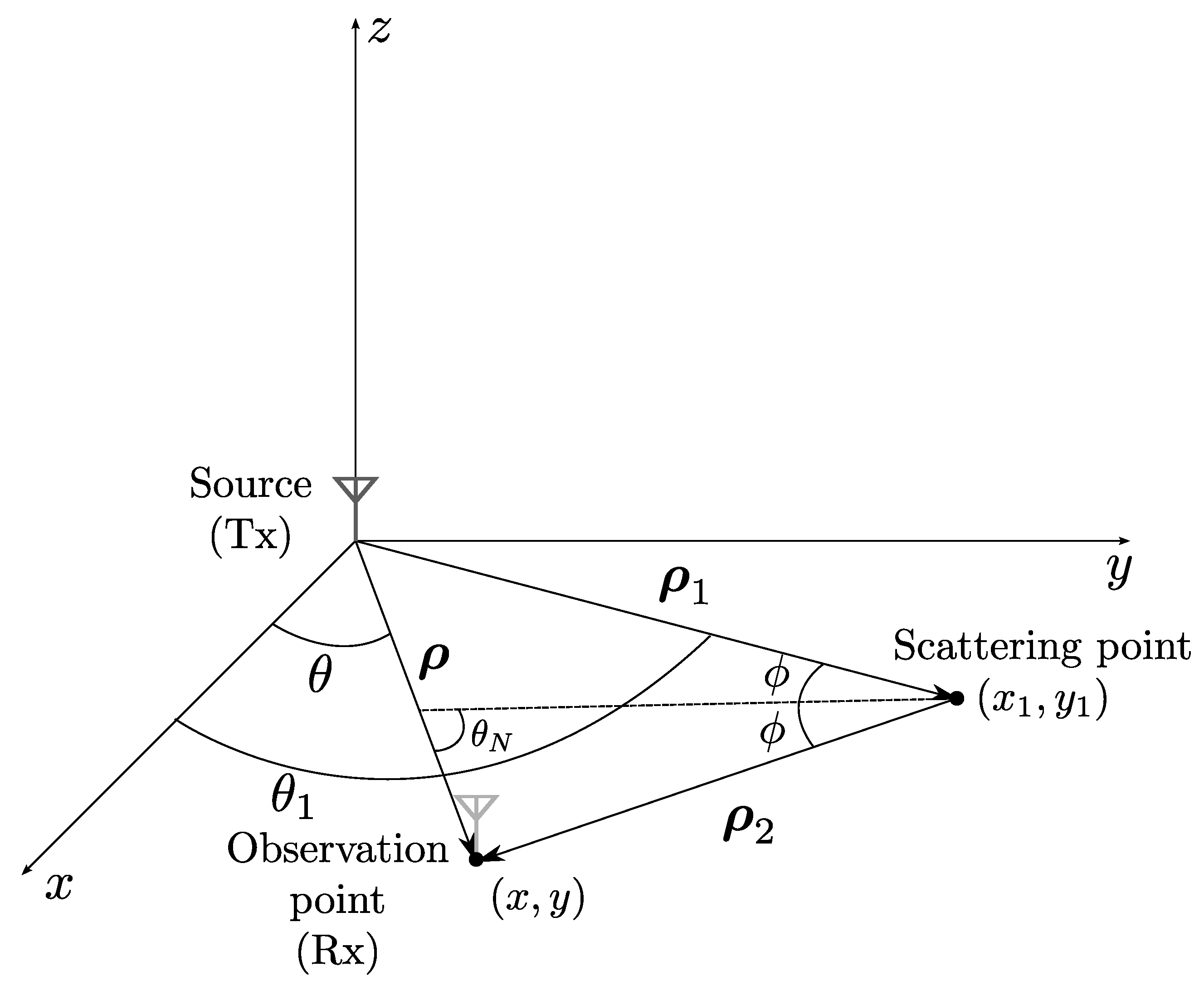
where indicates a two-dimensional spatial convolution in the -plane. The scattering geometry for the first-order electric field is depicted in Figure 1.
If a Fourier series representation of the ocean surface is considered, the surface displacement can be written as [30]
with being the wave vector for the ocean surface and being the angular frequency obtained from the dispersion relation of ocean surface gravity waves [27]. By substituting (8) into (6), expanding the exponential that contains the arbitrary height factor into a power series and applying an asymptotic perturbation expansion to both the Fourier components of the ocean surface and the electric fields using the surface slope as the perturbation parameter [31], it can be shown that the received first-order electromagnetic and second-order hydrodynamic electric fields contain terms equivalent to those for the small-height case, but an extra term appears in the second-order derivation which relates the first-order cross-section and the arbitrary height factor. The new term can be written as [28]
Comparing the double integrals in (9) with those in the first-order electric field expression in [16,17], it is evident that they are identical. Therefore, following the same procedure detailed in [17] for the first-order bistatic electric field, the following expression is obtained as
where is defined as
is the bistatic angle, defined as the bisection of the angle between and , and is the vector between the transmitter and receiver, shown in Figure 1.
If, similarly to [16,18], an inverse Fourier transform with respect to the radar frequency is applied to (10) while using the associative property of the convolution, the following expression can be obtained:
Again, it can be easily observed that the time convolution () inside the braces is similar to the one presented in Equation (5) of [18], with the exception of the time-dependent exponential term for the Fourier series expansion of the ocean surface; although this term will not affect the inverse Fourier transform, it might have an effect on the final convolution. It is easy to show that the additional time-dependent exponential term does not affect the resulting expression, since the added terms in the final expression are significantly smaller than the rest of the terms in the expression. Therefore, substituting the resulting expression for the first-order time-varying electric field in [18] for a pulsed radar source, the expression in (11) becomes
where is the sampling function, defined as
and is the patch width on the ocean surface, defined for a pulse radar as
with c being the speed of light and being the radar pulse width. Here, it should be noted that the zero-subscripts in , , and indicate that the scattering patch is considered to be sufficiently small, allowing variable values at the center of the scattering patch to be taken as representative of their values on the whole patch [32]. Consequently, is defined as
On the other hand, the zero-subscripts in , , and indicate that the radar transmitting frequency is considered constant during the radar operation. As explained in [16,18], the Sommerfeld attenuation function does not present significant variations with respect to radar frequency for typical bandwidths in a pulsed HF radar operation, allowing the frequency in to be considered constant and equal to the center-transmitting angular frequency . Similarly, it is easy to verify through dimensional analysis that variations in the arbitrary height factor with respect to radar frequency are very small, allowing it to be redefined as , where .
In order to obtain the expression for the time-varying bistatic electric field over the ocean surface, the arbitrary height factor must be further addressed. From the definition in (7), and taking the first-order expression for the ocean surface expansion appearing in (8), it can be shown that
Substituting (13) into (12) and performing the convolution, the time-varying bistatic electric field for arbitrary heights is obtained:
where , , and are functions of .
Here, a differentiation must be made between the two different time-related variables t and . In [16], Walsh and Gill differentiated between the “time of observation” and the “experiment time” t for successive pulses, while here, will be treated as the “radar time” and t as the “ocean surface time”. Since radar-dependent events occur on a different time scale from that of the events of the ocean surface, they can be treated as two independent variables, even though both variables refer to time.
3. First-Order Radar Cross-Section of the Ocean Surface with Arbitrary Heights
From [18], the autocorrelation for a general electric field, denoted as , can be defined as
such that coincides with the average power at the receiver. In (15), is the effective free-space aperture of the receiver, is the intrinsic impedance of the free space, is the expected value operator, and the bar over the electric field indicates its conjugate. Expanding (15) into its different perturbation orders and knowing that, for the ocean surface [27]
where are the -th-order terms of the asymptotic expansion of the ocean surface and are their corresponding ocean wave spectra, it is easy to show that the only surviving terms of the autocorrelation are the ones multiplying fields of the same order:
where
and
are respectively the autocorrelations of the first-order electric field, second-order correction to the first-order electric field, and second-order hydrodynamic electric field, with the first-order and second-order hydrodynamic electric fields defined as in [17]. Therefore, the correction term for the bistatic electric field for the ocean surface with arbitrary heights presented here does not affect the form of the radar cross-section expressions previously derived in [18]. Thus, taking the autocorrelation of (14) according to the expression presented in (16) and proceeding with the derivations, the following expression is obtained:
From [18], it is known that
where is the power spectral density of the electric field, defined as the Fourier transform of the autocorrelation with respect to , and is the radar cross-section of the scattering object. After obtaining the power spectral density from the autocorrelation in (17), knowing from the bistatic scattering geometry that , where is the direction normal to the scattering ellipse at the scattering patch, and that [18]
the second-order correction to the first-order bistatic radar cross-section for an ocean surface with arbitrary heights can be obtained by comparison with (18) as
4. Simulation Results
In order to assess the impact of the newly-derived term in the total radar cross-section of the ocean surface, simulations were conducted in both high and low sea states. In both cases, two different bistatic configurations were chosen, with two different dominant wave directions, such that both the effects of wave directions and bistatic configurations on the results could be analyzed.
Before proceeding with the radar cross-section simulations, the validity of the second-order correction to the first-order term must be investigated, since the small-slope approximation still applies to (19). For this purpose, a number of total mean-square slope models proposed in the literature were used to compute the root-mean-square slope for the different ocean conditions used in the simulations. These models were developed empirically, using ocean surface measurements obtained with different instruments such as aerial photographs [33] and GPS-R [34]. The resulting total root-mean-square slopes for each of the simulated meteorological conditions are presented in Table 1, where is the wind speed measured at 19.5 m above the ocean surface.
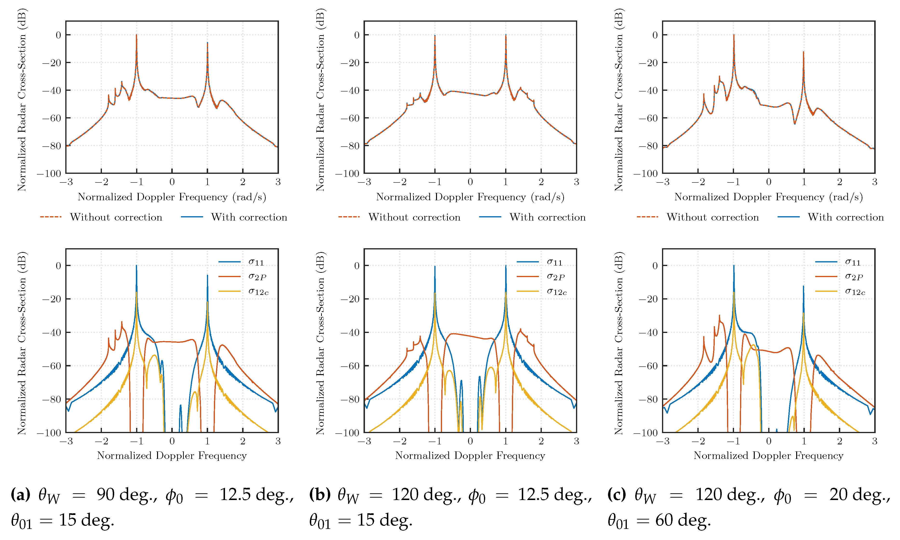
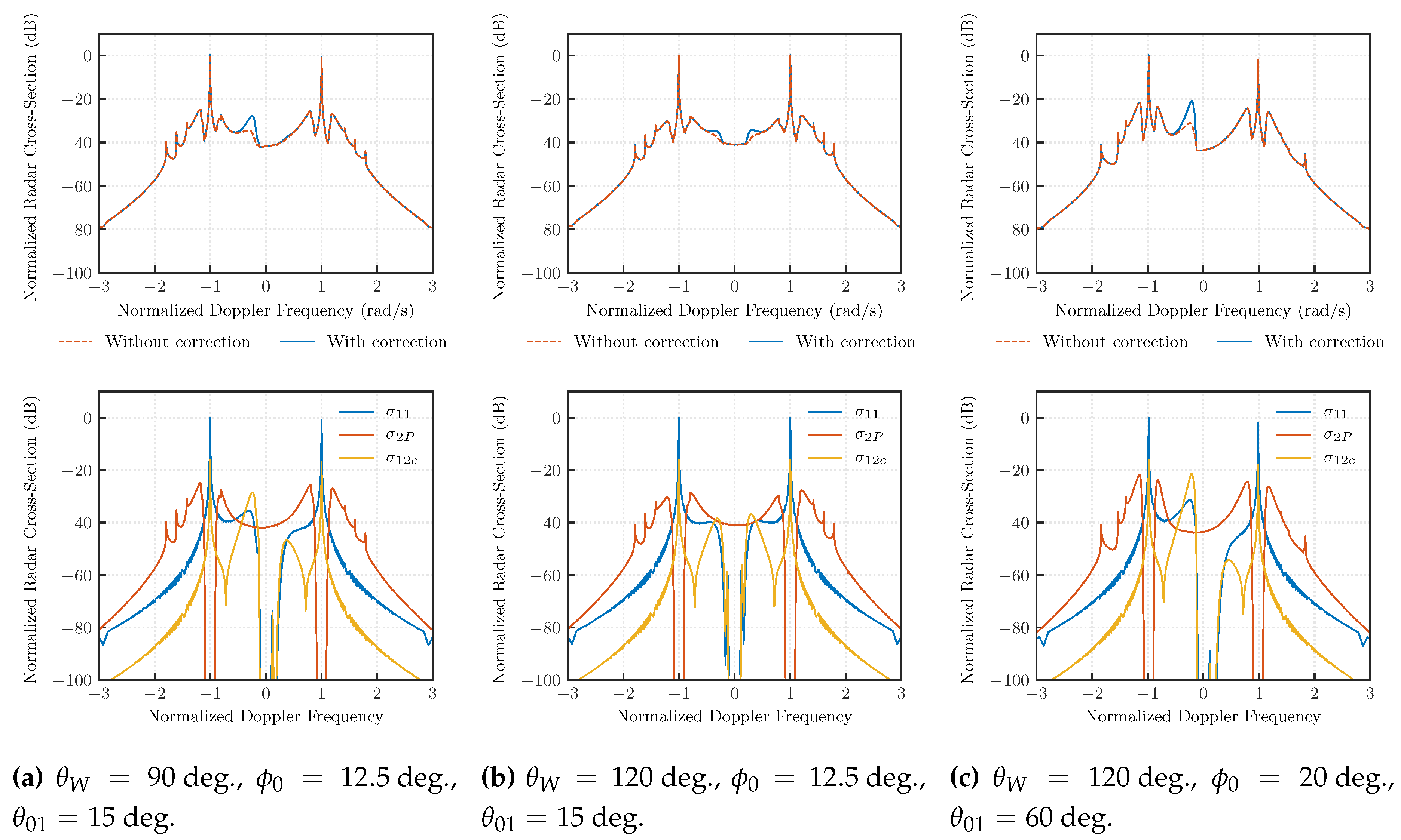
For the radar cross-section simulations, the Pierson–Moskowitz (PM) spectrum was chosen as the nondirectional spectral model of the ocean surface [38], with a cosine-power model for the directional factor [39] using the frequency-dependent wave-spreading factor proposed in [40]. Figure 2 and Figure 3 present the radar cross-section simulation results for low and high sea states, respectively. In the presented results, and respectively indicate the first- and second-order radar cross-sections of the ocean surface.
5. Discussion
In [26], the transition zone for the validity of the asymptotic perturbation method for roughness scales was defined for perturbation parameters between 0.4 and 0.7. Using the same intervals for the perturbation parameter chosen in the present work, it can be observed that all of the empirical models shown in Table 1 yielded total root-mean-square slopes below the lower bound of the transition zone, meaning that the validity condition for the perturbation theory has not been violated under either of the meteorological conditions used in the simulations.
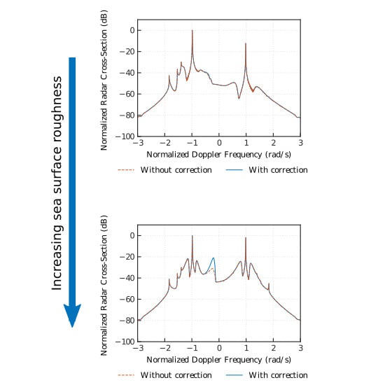
In observing the results in Figure 2 and Figure 3, it is clear that the proposed cross-section has little to no impact on the total cross-section at low sea states, with a maximum difference of less than , as shown in Figure 2b. This is an expected result, since the traditional second-order scattering theory is still valid for , even though the roughness scale is within the transition zone [26]. However, when observing the total radar cross-section at high sea states in Figure 3, where the roughness scale is above the upper limit of the transition zone, the correction term has an evident impact on the total radar cross-section, with a maximum difference of in Figure 3c.
The enhanced part in the total cross-section depends on the dominant wave direction of the ocean surface , as observed when comparing Figure 3a with Figure 3b, and on the bistatic radar configuration, as evidenced in analyzing Figure 3b,c. The maximum difference between the total cross-sections with and without the additional term on the presented results is .
In addition, the effects of the additional term are mostly evident in the central part of the total cross-section, at Doppler frequencies close to ; this is due to natural limitations on the steepness of large ocean waves, as well as to restrictions on the wave slope that are still imposed in the present analysis.
6. Conclusions and Future Work
In the present work, the scattered electric field and radar cross-section for an ocean surface with arbitrary heights using a narrow-beam bistatic HF radar have been derived. Previously derived electric field expressions presented in [17] for the small-height condition still appear in the final result, but due to the removal of the small-height approximation, a new term appears. The new term is interpreted as a correction to the first-order cross-section for arbitrary heights. The radar cross-section due to the correction term is also derived following the procedure presented in [18], and is then simulated for low and high sea states, showing an impact on the total radar cross-section for high sea states. A similar analysis is currently under review for the monostatic case.
The present work shows that changes in the dominant wave direction of the ocean surface and the bistatic configuration impact the contribution of the correction term to the radar cross-section. Since the other terms of the radar cross-section are saturated at sufficiently high sea states, the correction term may provide input for determining the dominant wave direction at high sea states. More extensive work needs to be dedicated to the understanding of interactions between the bistatic configuration and dominant wave direction, as well as the correction term, determining thresholds above which the correction term should be considered, and how different bistatic configurations can be used in observing the ocean surface at large roughness scales.
It can also be noted that the simulations in the current work were carried out using a Pierson–Moskowitz spectral model, which implies the assumption of a fully-developed sea and does not depend on fetch [38]. Since changes in fetch are known to affect the mean squared slope of the ocean surface [27], the work of determining how changes in fetch affect the correction term, allowing its application to developing sea states, is ongoing.
Since the present work represents the first attempt to overcome the small-height constraint imposed on previously derived bistatic high-frequency radar cross-sections of the ocean surface, no practical applications of the proposed theory have been suggested in the present work, as more work must be done in the future for these applications to be devised. In addition, due to the lack of narrow-beam bistatic HF radar data available to the authors, which were measured under conditions that violate the limiting roughness scales of the theories proposed in the literature, or the lack of any other derived model for radar cross-section of the ocean surface at large roughness scales, a validation of the presented theory is not available in the current work. To validate the current theory, collaboration from the radio oceanography community is necessary, as multiple observations need to be conducted by users of narrow-beam bistatic HF radars at ocean conditions that violate the small-height assumption. In addition, efforts to establish bistatic operation of existing monostatic HF radars are ongoing on the coastline of Placentia Bay, Newfoundland, Canada in order to collect data for the validation of the presented theory.
Author Contributions
Conceptualization: M.T.S., W.H., and E.W.G.; methodology: M.T.S.; formal analysis: M.T.S.; investigation: M.T.S.; resources: W.H. and E.W.G.; data curation: M.T.S.; writing—original draft preparation: M.T.S.; writing—review and technical editing: M.T.S., W.H., and E.W.G.; visualization: M.T.S.; project administration: W.H.; supervision: W.H. and E.W.G.; funding acquisition: W.H. and E.W.G. All authors have read and agreed to the published version of the manuscript.
Funding
This work was supported by the Natural Sciences and Engineering Research Council of Canada (NSERC) under Discovery Grants to W. Huang (NSERC RGPIN-2017-04508 and RGPAS-2017-507962) and E. W. Gill (NSERC RGPIN-2015-05289).
Conflicts of Interest
The authors declare no conflict of interest.
References
- Crombie, D.D. Doppler spectrum of sea echo at 13.56 Mc./s. Nature 1955, 175, 681–682. [Google Scholar] [CrossRef]
- Barrick, D.E. HF radio oceanography—A review. Bound-Lay. Meteorol. 1978, 13, 23–43. [Google Scholar] [CrossRef]
- Hardman, R.L.; Wyatt, L.R. Inversion of HF radar Doppler spectra using a neural network. J. Mar. Sci. Eng. 2019, 7, 255. [Google Scholar] [CrossRef] [Green Version]
- Sun, W.; Huang, W.; Ji, Y.; Dai, Y.; Ren, P.; Zhou, P.; Hao, X. A vessel azimuth and course joint re-estimation method for compact HFSWR. IEEE Trans. Geosci. Remote Sens. 2019, 1–11. [Google Scholar] [CrossRef]
- Sun, W.; Huang, W.; Ji, Y.; Dai, Y.; Ren, P.; Zhou, P. Vessel tracking with small-aperture compact high-frequency surface wave radar. In Proceedings of the OCEANS 2019—Marseille, Marseille, France, 17–20 June 2019; pp. 1–4. [Google Scholar] [CrossRef]
- Pidgeon, V.W. Bistatic cross section of the sea. IEEE Trans. Antennas Propag. 1966, 14, 405–406. [Google Scholar] [CrossRef]
- Peterson, A.M.; Teague, C.C.; Tyler, G.L. Bistatic-radar observation of long-period, directional ocean-wave spectra with Loran A. Science 1970, 170, 158–161. [Google Scholar] [CrossRef]
- Teague, C.C. Bistatic-radar techniques for observing long-wavelength directional ocean-wave spectra. IEEE Trans. Geosci. Electron. 1971, 9, 211–215. [Google Scholar] [CrossRef]
- Teague, C.C.; Vesecky, J.F.; Fernandez, D.M. HF radar instruments, past to present. Oceanography 1997, 10, 40–44. [Google Scholar] [CrossRef]
- Barrick, D.E. The interaction of HF/VHF radio waves with the sea surface and its implications. In AGARD Conference Proceedings No. 77 on Electromagnetics of the Sea; Aerospace Research & Development (AGARD), Ed.; National Atlantic Threaty Organization (NATO): Washington, DC, USA, 1970; number AGARD-CP-77-70; pp. 18-1–18-25. [Google Scholar]
- Barrick, D.E. Remote sensing of sea state by radar. In Remote Sensing of the Troposphere; Derr, V., Ed.; U.S. Department of Commerce—National Oceanic and Atmospheric Administration: Boulder, CO, USA, 1972; Chapter 12; pp. 12-1–12-46. [Google Scholar]
- Johnstone, D.L. Second-Order Electromagnetic and Hydromagnetic Effects in High-Frequency Radio-Wave Scattering from the Sea. Ph.D. Thesis, Stamford, CA, USA, 1975. [Google Scholar]
- Anderson, S.J.; Anderson, W.C. Bistatic HF scattering from the ocean surface and its application to remote sensing of seastate. In Proceedings of the 1987 IEEE APS International Symposium, Blacksburg, VA, USA, 15–19 June 1987. [Google Scholar]
- Anderson, S.J.; Fuks, I.M.; Praschifka, J. Multiple scattering of HF radio waves propagating across the sea surface. Wave. Random Media 1998, 8, 283–302. [Google Scholar] [CrossRef]
- Anderson, S.J. Directional wave spectrum measurement with multistatic HF surface wave radar. In Taking the Pulse of the Planet: The Role of Remote Sensing in Managing the Environment. Proceedings (Cat. No.00CH37120); IEEE: Honolulu, HI, USA, 2000. [Google Scholar] [CrossRef]
- Walsh, J.; Gill, E.W. An analysis of the scattering of high-frequency electromagnetic radiation from rough surfaces with application to pulse radar operating in backscatter mode. Radio Sci. 2000, 35, 1337–1359. [Google Scholar] [CrossRef] [Green Version]
- Gill, E.W.; Walsh, J. Bistatic form of the electric field equations for the scattering of vertically polarized high-frequency ground wave radiation from slightly rough, good conducting surfaces. Radio Sci. 2000, 35, 1323–1335. [Google Scholar] [CrossRef]
- Gill, E.W.; Walsh, J. High-frequency bistatic cross sections of the ocean surface. Radio Sci. 2001, 36, 1459–1475. [Google Scholar] [CrossRef]
- Gill, E.W.; Huang, W.; Walsh, J. On the development of a second-order bistatic radar cross section of the ocean surface: A high-frequency result for a finite scattering patch. IEEE J. Ocean. Eng. 2006, 31, 740–750. [Google Scholar] [CrossRef]
- Chen, S.; Huang, W.; Gill, E.W. First-order bistatic high-frequency radar power for mixed-path ionosphere-ocean propagation. IEEE Geosci. Remote Sens. Lett. 2016, 13, 1940–1944. [Google Scholar] [CrossRef]
- Ma, Y.; Gill, E.W.; Huang, W. First-order bistatic high-frequency radar ocean surface cross-section for an antenna on a floating platform. IET Radar Sonar Navig. 2016, 10, 1136–1144. [Google Scholar] [CrossRef] [Green Version]
- Ma, Y.; Huang, W.; Gill, E.W. The second-order bistatic high-frequency radar cross section of ocean surface for an antenna on a floating platform. Can. J. Remote Sens. 2016, 42, 332–343. [Google Scholar] [CrossRef]
- Ma, Y.; Gill, E.W.; Huang, W. Bistatic high-frequency radar ocean surface cross section incorporating a dual-frequency platform motion model. IEEE J. Ocean. Eng. 2018, 43, 205–210. [Google Scholar] [CrossRef]
- Grosdidier, S.; Forget, P.; Barbin, Y.; Gúerin, C.A. HF bistatic ocean Doppler spectra: simulation versus experimentation. IEEE Trans. Geosci. Remote Sens. 2014, 52, 2138–2148. [Google Scholar] [CrossRef] [Green Version]
- Barrick, D.E. Theory of HF and VHF propagation across the rough sea, 1, the effective surface impedance for a slightly rough highly conducting medium at grazing incidence. Radio Sci. 1971, 6, 517–526. [Google Scholar] [CrossRef]
- Wyatt, L.R. High order nonlinearities in HF radar backscatter from the ocean surface. IEE Proc. Radar Sonar Navig. 1995, 142, 293. [Google Scholar] [CrossRef]
- Massel, S.R. Ocean Surface Waves: Their Physics and Prediction, 3rd ed.; World Scientific Publishing: Singapore, 2017; p. 776. [Google Scholar]
- Silva, M.T.; Gill, E.W.; Huang, W. First-order high-frequency scattering for ocean surfaces with large roughness scales. Presented at the 28th Annual Newfoundland Electrical and Computer Engineering Conference (NECEC 2019), St. John’s, NL, Canada, 19 November 2019. [Google Scholar]
- Walsh, J. Asymptotic expansion of a Sommerfeld integral. Electron. Lett. 1984, 20, 746. [Google Scholar] [CrossRef]
- Weber, B.L.; Barrick, D.E. On the nonlinear theory for gravity waves on the ocean’s surface. Part I: derivations. J. Phys. Oceanogr. 1977, 7, 3–10. [Google Scholar] [CrossRef]
- Hasselmann, K. On the non-linear energy transfer in a gravity-wave spectrum Part 1. General theory. J. Fluid Mech. 1962, 12, 481. [Google Scholar] [CrossRef]
- Gill, E.W. The Scattering of High Frequency Electromagnetic Radiation from the Ocean Surface: An Analysis Based on a Bistatic Ground Wave Radar Configuration. Ph.D. Thesis, Memorial University of Newfoundland, St. John’s, NL, Canada, 1999. [Google Scholar]
- Cox, C.; Munk, W. Measurement of the roughness of the sea surface from photographs of the sun’s glitter. J. Opt. Soc. Am. 1954, 44, 838. [Google Scholar] [CrossRef]
- Gleason, S.; Zavorotny, V.U.; Akos, D.M.; Hrbek, S.; PopStefanija, I.; Walsh, E.J.; Masters, D.; Grant, M.S. Study of surface wind and mean square slope correlation in hurricane Ike with multiple sensors. IEEE J. Sel. Topics Appl. Earth Observ. Remote Sens. 2018, 11, 1975–1988. [Google Scholar] [CrossRef]
- Wu, J. Mean square slopes of the wind-disturbed water surface, their magnitude, directionality, and composition. Radio Sci. 1990, 25, 37–48. [Google Scholar] [CrossRef]
- Hwang, P.A. Wave number spectrum and mean square slope of intermediate-scale ocean surface waves. J. Geophys. Res. 2005, 110. [Google Scholar] [CrossRef] [Green Version]
- Katzberg, S.J.; Torres, O.; Ganoe, G. Calibration of reflected GPS for tropical storm wind speed retrievals. Geophys. Res. Lett. 2006, 33. [Google Scholar] [CrossRef] [Green Version]
- Pierson, W.J.; Moskowitz, L. A Proposed Spectral form for Fully Developed Wind Seas Based on the Similarity Theory of S. A. Kitaigorodskii; Technical Report; U.S. Naval Oceanographic Office: New York, NY, USA, 1963. [Google Scholar]
- Longuet-Higgins, M.S. The effect of non-linearities on statistical distributions in the theory of sea waves. J. Fluid Mech. 1963, 17, 459. [Google Scholar] [CrossRef]
- Mitsuyasu, H.; Tasai, F.; Suhara, T.; Mizuno, S.; Ohkusu, M.; Honda, T.; Rikiishi, K. Observations of the directional spectrum of ocean waves using a cloverleaf buoy. J. Phys. Oceanogr. 1975, 5, 750–760. [Google Scholar] [CrossRef] [Green Version]
Figure 1.
Scattering geometry for the bistatic first-order electric field.

Figure 2.
Total bistatic radar cross-section and its components for three different bistatic geometries and wave directions at low sea states. Wind speed , radar frequency , and roughness scale .
Figure 2.
Total bistatic radar cross-section and its components for three different bistatic geometries and wave directions at low sea states. Wind speed , radar frequency , and roughness scale .

Figure 3.
Total bistatic radar cross-section and its components for three different bistatic geometries and wave directions at low sea states. Wind speed , radar frequency , and roughness scale .
Figure 3.
Total bistatic radar cross-section and its components for three different bistatic geometries and wave directions at low sea states. Wind speed , radar frequency , and roughness scale .


Table 1.
Total root-mean-square slopes for simulated meteorological conditions using different slope models.
Table 1.
Total root-mean-square slopes for simulated meteorological conditions using different slope models.
| MSS Slope Model | Total Root-Mean-Square Slope | |
|---|---|---|
| m/s | m/s | |
| Cox and Munk (1954) [33] | 0.22206 | 0.31477 |
| Wu (1990) [35] | 0.22319 | 0.30573 |
| Hwang (2005) [36] | 0.22252 | 0.32197 |
| Katzberg, Torres and Ganoe (2006) [37] | 0.15098 | 0.18104 |
| Gleason et al. (2018) [34] | 0.16119 | 0.18041 |
© 2020 by the authors. Licensee MDPI, Basel, Switzerland. This article is an open access article distributed under the terms and conditions of the Creative Commons Attribution (CC BY) license (http://creativecommons.org/licenses/by/4.0/).
Share and Cite
MDPI and ACS Style
Silva, M.T.; Huang, W.; Gill, E.W. Bistatic High-Frequency Radar Cross-Section of the Ocean Surface with Arbitrary Wave Heights. Remote Sens. 2020, 12, 667. https://doi.org/10.3390/rs12040667
AMA Style
Silva MT, Huang W, Gill EW. Bistatic High-Frequency Radar Cross-Section of the Ocean Surface with Arbitrary Wave Heights. Remote Sensing. 2020; 12(4):667. https://doi.org/10.3390/rs12040667
Chicago/Turabian StyleSilva, Murilo Teixeira, Weimin Huang, and Eric W. Gill. 2020. "Bistatic High-Frequency Radar Cross-Section of the Ocean Surface with Arbitrary Wave Heights" Remote Sensing 12, no. 4: 667. https://doi.org/10.3390/rs12040667
Note that from the first issue of 2016, this journal uses article numbers instead of page numbers. See further details here.