Structural Building Damage Detection with Deep Learning: Assessment of a State-of-the-Art CNN in Operational Conditions


1
Faculty of Geo-Information Science and Earth Observation (ITC), University of Twente, 7500 AE Enschede, The Netherlands
2
Politecnico di Torino, Department of Architecture and Design, 10125 Torino, Italy
*
Author to whom correspondence should be addressed.
Remote Sens. 2019, 11(23), 2765; https://doi.org/10.3390/rs11232765
Submission received: 23 October 2019
/
Revised: 19 November 2019
/
Accepted: 20 November 2019
/
Published: 24 November 2019
(This article belongs to the Special Issue Image Processing and Analysis: Trends in Registration, Data Fusion, 3D Reconstruction and Change Detection)
Abstract
:Remotely sensed data can provide the basis for timely and efficient building damage maps that are of fundamental importance to support the response activities following disaster events. However, the generation of these maps continues to be mainly based on the manual extraction of relevant information in operational frameworks. Considering the identification of visible structural damages caused by earthquakes and explosions, several recent works have shown that Convolutional Neural Networks (CNN) outperform traditional methods. However, the limited availability of publicly available image datasets depicting structural disaster damages, and the wide variety of sensors and spatial resolution used for these acquisitions (from space, aerial and UAV platforms), have limited the clarity of how these networks can effectively serve First Responder needs and emergency mapping service requirements. In this paper, an advanced CNN for visible structural damage detection is tested to shed some light on what deep learning networks can currently deliver, and its adoption in realistic operational conditions after earthquakes and explosions is critically discussed. The heterogeneous and large datasets collected by the authors covering different locations, spatial resolutions and platforms were used to assess the network performances in terms of transfer learning with specific regard to geographical transferability of the trained network to imagery acquired in different locations. The computational time needed to deliver these maps is also assessed. Results show that quality metrics are influenced by the composition of training samples used in the network. To promote their wider use, three pre-trained networks—optimized for satellite, airborne and UAV image spatial resolutions and viewing angles—are made freely available to the scientific community.
1. Introduction
The localization of damaged buildings in the immediate hours after a disastrous event is one of the first and most important tasks of the emergency response phase [1,2]. In this regard, remote sensing is a cost effective and rapid way to inspect the area and exploit the acquired information to organize prompt actions [3].
Optical satellite imagery has been the most widely adopted data source for building damage detection, due to the possibility to image every area of the Earth, with different sensors and spatial resolution, in a few hours/days from the tasking request. Mechanisms and services such as the International Charter “Space and Major Disasters” (IC) and the Copenicus Emergency Management Service (CEMS) have been exploiting these images for the last 20 years [4]. However, the intrinsic limitations of vertical imagery in identifying structural damages to buildings [5,6] and the frequent presence of cloud cover, have limited the adoption of automated procedures in favor of traditional manual methods that may be affected by subjectivity in the identification of damages from imagery [7] (despite efforts in developing international standard and guidelines for building damage assessment [8]). Airborne (nadir and oblique) images have demonstrated their higher flexibility [9], surveying large areas with high resolution and complete data capture. However, manned airplanes are often unavailable in remote areas, especially in the immediate hours after an emergency; in most cases, airborne images to assess the damages and the economic losses only become available several days after the catastrophic event (therefore, supporting the cleanup and rehabilitation phases rather than emergency response).
The recent proliferation of UAV (Unmanned Aerial Vehicles) technology has provided an additional instrument for building damage detection, as confirmed by the growing number of image data collected in the aftermath of a disaster in the last few years. Despite their flexibility in terms of data capture, their image quality and availability (with several million UAV of sufficient imaging quality being sold yearly worldwide) are poor—the spatial extent that they can cover is severely limited when compared to satellite and manned aerial platforms. UAV can, therefore, be considered a good instrument for local rescue teams [10] rather than for synoptic mapping of the affected area.
Automated disaster mapping is still an open research topic. Different types of man-made and natural disasters (i.e., earthquake, explosion, typhoon, flooding, tsunami, etc.) affect building structures differently, often producing distinctive evidence in remotely sensed data. Visible structural building damages can look completely different depending on the disaster type considered, and a general approach that is automatically and accurately able to cope with all different typologies of disasters is not in reach at the moment.
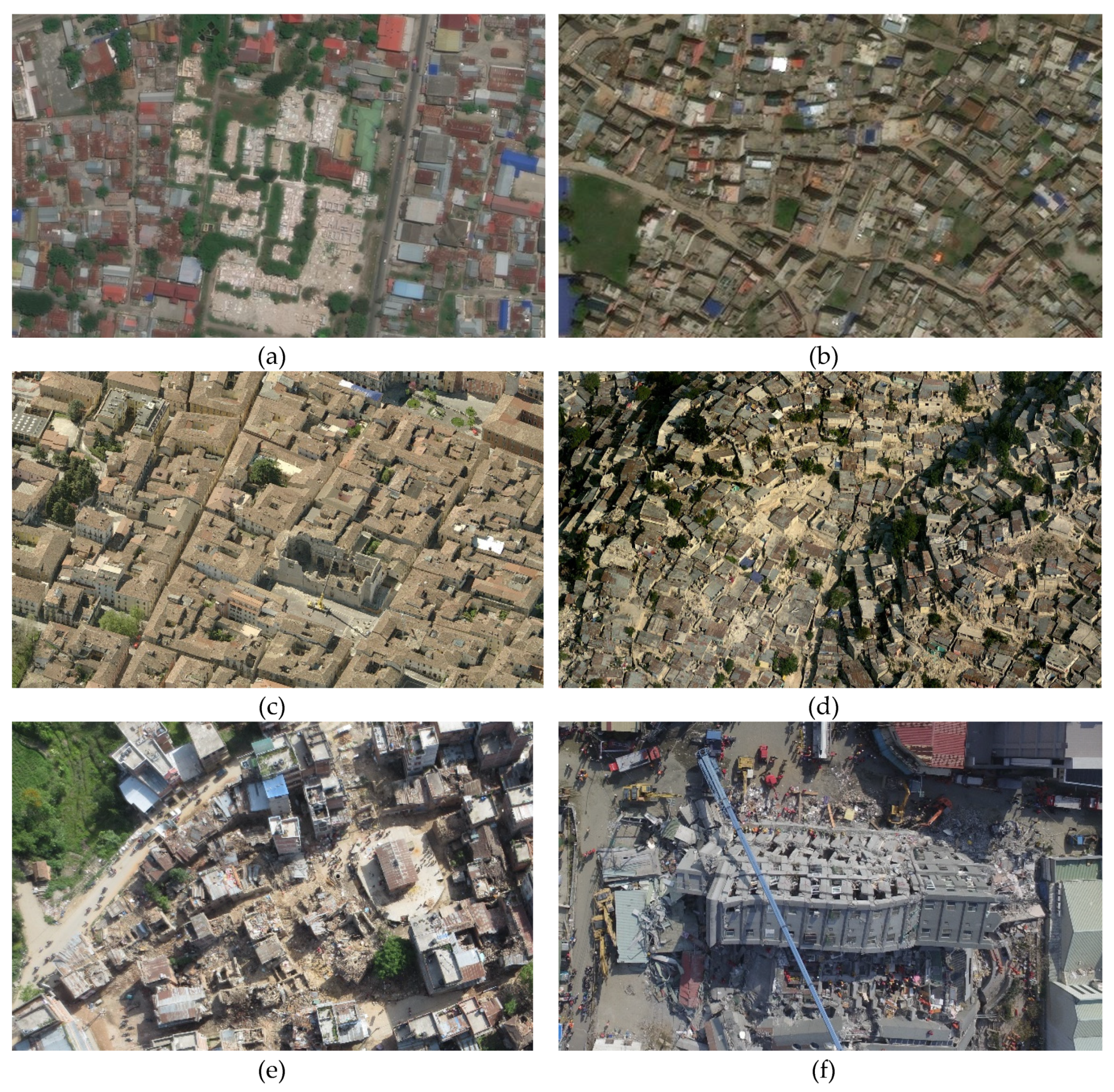
In this paper, we only focus on visible damages caused by earthquakes and explosions, as they produce similar signatures. Nevertheless, in these rather clear cases, structural damage identification is still not a trivial task. The high variability in spatial and spectral resolution, the even larger variability in the image quality resulting from the different sensors, off-nadir angles and environmental conditions (i.e., haze, sub-optimal illumination, etc.) represent the main challenge in the implementation of efficient and robust algorithms. Additionally, debris and building damages look completely different according to the type of building: concrete buildings, mansory or buildings made from natural materials are characterised by different features and patterns when captured in an image (Figure 1).
Different automated approaches have been proposed in the past, using supervised and unsupervised classification techniques [9,11,12,13]. Most approaches have been conceived to detect damages on specific areas and using a single specific data resolution, while a very limited number of contributions dealt with the use of multi-resolution sources [14,15].
In recent years, the rapid development of deep learning techniques has revolutionized the approaches for segmentation and classification of data acquired by different sensors and resolutions. Traditional damage detection methods are being outperformed in terms of accuracy by Convolutional Neural Networks (CNN) in particular [16]. However, their adoption in real cases has been limited so far, due to the continuous lack of clarity in terms of their performance in more realistic and operational conditions. To the best of the authors’ knowledge, no systematic study exists on the capability of deep learning building damages algorithms to deliver reliable results in operational conditions (i.e., use of pre-trained networks with limited or no ad-hoc training and delivery of the analysis results within a few hours of image acquisition).
Compared to many other remote sensing applications, where datasets are abundant, an additional challenge is the limited number of publicly available large repositories tailored to emergency mapping to allow the training and testing of new solutions. In this regard, the number of companies or independent surveyors collecting data on disaster areas have grown substantially in recent years, but only few datasets are publicly available. Those are then limited to a specific data resolution [17] or a few test cases [18], and are thus often insufficient for a thorough validation of deep learning approaches. We have collected a wide number of datasets acquired by different sensors and with different spatial resolutions in the framework of the response to the major seismic events during the last decade.
In the framework of two EU funded FP7 projects (Reconass [19] and Inachus [20]), several algorithms, mostly based on CNN, have been developed, improving the detection of structural damages caused by earthquakes or explosions [15,16,21,22], which generate comparable damage signatures. Considering these two event typologies, this paper investigates the performances of current CNN for building damage detection in realistic operative conditions, investigating their performance in terms of (i) transfer learning and (ii) running time. In (i), it is assessed to what extent a pre-trained network can successfully identify damages (with or without limited training) on a new location characterized by different building typologies and environmental conditions. In (ii), the processing time is considered with respect to the usual constraints of emergency mapping.
A novel CNN network architecture is proposed, building on previous works and experiences, taking advantage of the latest developments in deep learning, and considering a good trade-off between accuracy and running time. The same network was trained using different data resolutions (satellite, airborne and UAV images). Although the developed network outperforms previous approaches in terms of accuracy and running time, the aim of this contribution is not to assess its absolute performance, but to critically discuss the suitability of current CNNs in operational activities: the adopted network is representative of the current state-of-the-art deep learning performances for this task. The available datasets were used to design different tests (in all three data resolutions), and to assess the behavior of the network with completely new data or with reduced fine-tuning, simulating realistic time-constrained conditions. Most of the datasets used cannot be publicly shared, but we release the best pre-trained models presented in the paper to the community to allow their further use (see the Supplementary Material of this paper).
The paper is organized as follows: Section 2 summarizes the existing methods for building damage detection from remote sensing imagery. The tested CNN architecture is described in Section 3. The used dataset (Section 4) and the tests conducted to validate the used network (Section 5) are then reported. Section 6 and 7 provide a discussion and the conclusions, respectively.
2. Existing Building Damage Detection Approaches
In recent decades, different space, air and ground platforms equipped with optical [23,24], radar [25,26] and LiDAR [27,28] sensors have been used to collect data for building damage identification. However, the majority of these approaches focused on the use of optical data from satellite and airborne data, relating damage to the visible patterns in the images. As largely confirmed in the literature [29], the appearance of damages caused by earthquakes and explosions can substantially change according to four main parameters: (i) the used platform and sensor, (ii) image resolution, (iii) type of acquisition and viewing angle (nadir, oblique) and (iv) typology of building damages to be detected. In the past decade, different approaches were proposed according to those four parameters, exploiting (as an example) co-occurrence matrices on satellite images [30] or morphological-scale spaces [31], or aiming at optimizing the detection of specific building elements such as bricks and roof tiles [32]. Other approaches have used active learning to improve the quality of the classification [33]. Higher image resolutions increase the level of detail of the images and, as a consequence, the complexity and variability of the objects that can be described. Object-based image analysis (OBIA) has, therefore, been adopted in several approaches [34] to reduce the complexity of the detection task: these approaches work on “homogenous” (i.e., segmented) regions and reduce the computational time, computing features on regions and not at pixel level. In some approaches, instead of using only 2D images, 3D features have also been extracted from photogrammetric point cloud regions to detect deformations [35].
The use of traditional handcrafted features has shown severe limits, prompting the development of more robust classifiers through bag-of-words models [36]. More recently, the growing popularity of CNN for other recognition tasks (particularly in terrestrial imagery) has led to the wide adoption of these approaches in building damage detection. Several architectures have been proposed to improve the debris detection performance by implementing more complex and advanced solutions [21,37]. Recent approaches have made use of convolutional autoencoders to cope with a reduced number of samples [38], which has led to some improvements in the classification of damages. However, the limited availability of datasets has constrained these developments to very specific datasets with defined resolutions and test locations. Other approaches have tried to work with multi-temporal data to reliably detect changes after catastrophic events [39,40], but their practical use has been limited by the availability of pre-event data. To cope with the lack of reference data, recent studies [41] applied CNNs to extract building footprints from pre-event imagery, as well as to update those outlines after a disaster event [42]. The integration of CNN and 3D features derived from photogrammetric point clouds [16] has shown encouraging results, with the drawback of requiring more time for the classification. The recent introduction of a multi-resolution approach, embedding the use of different data resolutions in a unique architecture [15], has shown promising results: the first layers of the network are trained using samples from different resolutions, and resolution-specific data are used only in the last layers to optimize the CNN on this specific data resolution. This network has provided more robust results than previous works, but it has shown some limits in terms of processing time and ease of use.
3. The Adopted Convolutional Neural Network
The CNN proposed in this paper takes advantage of the expertise built in previous works and embeds the architectures available in the computer vision literature, specifically: (i) dense connections and (ii) dilated convolutions.
The dense connections [43] concatenate the feature maps of preceding layers with the input of a given layer: each of them receives the feature information from all preceding layers. These densely connected networks are built by stacking dense blocks composed of convolutional sets and introducing transitional blocks among them to downscale the feature maps through pooling. The concatenation of the feature maps is performed within each of these dense blocks (see Figure 2).
This kind of architecture has fewer filters in each convolution set, which becomes particularly relevant when we increase the depth of a network [44]. The number of filters is usually tied to a pre-defined growth rate applied to each of the dense blocks. Densely connected networks also have the advantage of significantly reducing the number of parameters used to train compared to residual networks [45]: training is easier compared to other network architectures as each layer has access to the gradients from the loss function and the original input image. In addition, the reduced number of parameters decreases the risk of overfitting (particularly, with relatively limited datasets), and the running time of the detection process is shorter than other networks such as in [15]. This last element is crucial in the generation of fast damage maps in the initial hours after an emergency.
The dilated convolutions [46] allow to capture the spatial context of the image patches using a “gapped” kernel for convolution filtering instead of a contiguous one. The spatial context was previously captured by down-sampling the feature maps through pooling. On the contrary, dilated convolutions capture the context, enlarging the receptive field with this type of kernel: this allows for preservation of the finer details in the images that would be lost in the down-sampling of the feature maps [47].
This property has been shown to be particularly relevant to capture the texture of building debris, especially when different spatial resolutions (i.e., Ground Sampling Distances—GSD) are considered, varying the size of the used receptive field in the image. The use of dilations is also very useful to embed in the network the study of damage cues and their context in all the levels of resolution.
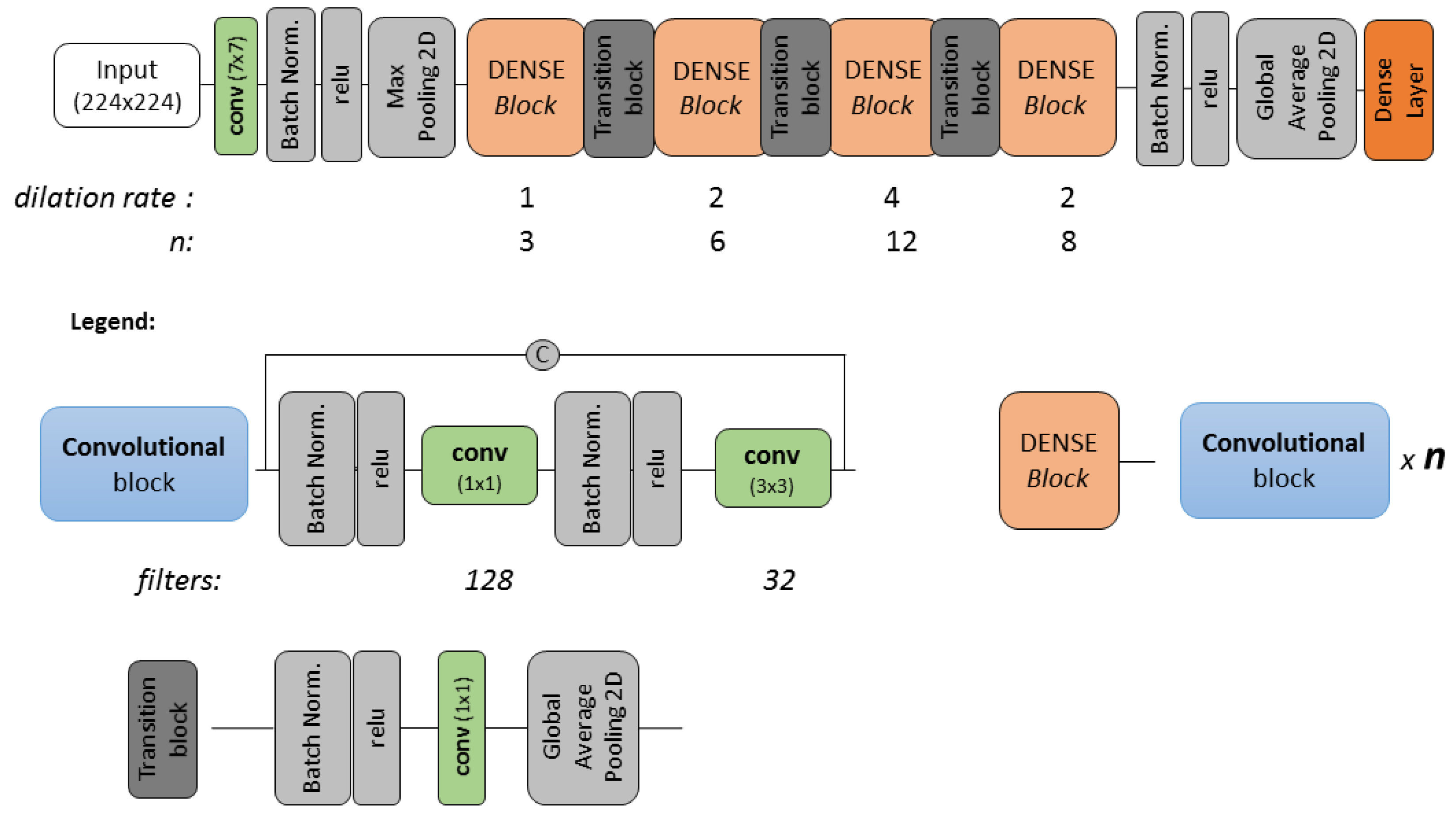
The adopted network (Figure 2) is an adaptation of densenet121 [43]. This network is composed of sets of convolutional blocks, denominated as dense blocks. Each convolutional block is composed of a sequence of batch normalization, ReLU, (1 × 1) convolution, another batch normalization, ReLU and a final (3 × 3) convolution (see Figure 2). These convolutional blocks are repeated n times (n in Figure 2), where the feature maps within each of these dense blocks are concatenated. The downscaling of the feature maps occurs in the transitional blocks where the global average pooling with stride 2 is performed. The original configuration of the densenet121 contains four blocks, where the number of convolutional blocks per block is 6, 12, 24, 16, respectively. In experimental tests, it was noticed that halving the number of blocks (i.e., 3, 6, 12, 8, as in Figure 2) did not impact the accuracy metrics on a validation dataset, and it could further attenuate the overfitting. The decrease in the number of convolutional blocks was followed by a change in the number of filters considered in each convolution set. In densenet121, the number of filters changes according to the growth rate, while in this implementation, this value is constant (as indicated in Figure 2): such modification further decreased the number of parameters without decreasing the quality of the model, as demonstrated in preliminary tests.
The dilation rate was set considering an increasingly larger receptive field (up to 4 dilation rate), followed by a decrease in the last set of dense blocks. The gradual increase of the dilation rate may introduce an aliasing effect on the feature maps, while the decrease of such a dilation rate in the last set of dense blocks aims at attenuating this problem [46]. Moreover, the decrease in the dilation rate re-captures more localized features, which might not have been considered previosly due to the increased dilation rate.
The batch size of the network was 16: in experimental tests, it was determined that a larger batch size could lead to a faster convergence of the network without reaching the same quality in the results. The Adam optimizer with a 0.01 learning rate was adopted during the training [48] for the models trained from scratch, and 0.001 for the fine-tuning ones.
Considering the fine-tuning of the network, it was observed from experimental tests that adding a dense layer at the end of the network was more useful than re-training the last layers (i.e., last dense block) of the original network. In the fine-tuning, all the convolutional weights of the pre-trained model were fixed and only this dense layer of size 512 was trained with the target location image samples. Data augmentation was also used: horizontal flips, image normalization, small rotations and small shifts were applied to the training samples. Only image normalization was used on the validation data.
The network performs a patch-based detection of damaged areas. The input is, therefore, given by a 224 × 224 pixel patch. As the resolution of the used data varies with the sensor used, a similar footprint size on the ground was used for the different resolution, adopting a 50×50, 80×80 and 120 × 120 pixel patches for satellite, airborne and UAV data, respectively. These were then resized to the input size of 224 × 224, maintaining the aspect ratio to fit this template. The input size of the original densenet121 was maintained, and it can be more easily adaptable to different data resolutions: the downscaling of the feature maps within the network maintains the same size as the original densenet paper. The reduction of the input patch size in the network would require a different architecture with less pooling layers, as the final feature map size is only 7 × 7 pixels. Preliminary tests showed that the use of different input patch sizes for each resolution did not provide significant improvements in the detection task, while zero-padding (instead of resampling) generally worsened the results.
4. Data Used
The data used were collected by the authors in the last few years, and they include both open-source and commercial imagery. These images can be categorized into three different groups, according to their spatial resolution: satellite, airborne and UAV images. As depicted in Table 1, very different locations, dates and sensors were included in each group. This resulted in a large variability in image quality, in the environmental conditions and typology of building damage depicted in the images. The GSD also varies within each group.
The approach presented in this paper classifies image patches as damaged or intact. A patch-based approach allows for incorporation of the context of a damaged region and to ease the computational cost and the image labelling tasks. The ground truth was generated, which identified the visible damages and intact areas by manual photointerpretation. The damaged regions (i.e., instances) were identified corresponding to rubble piles and debris that could be identified in all the considered resolutions. The intact areas were selected considering different objects in the scene and the specific characteristic of the dataset (i.e., image quality, resolution, etc.). A grid of different size according to the data resolution (i.e., 50 × 50 pixel, 80 × 80 pixel 120 × 120 pixel for satellite, airborne and UAV, respectively) was then used to generate the image patches: each patch was labelled as damaged if more than 40% of its pixels were identified in the damage mask [15].
A balanced number of intact and damaged samples were extracted from each data category, preventing problems due to uneven samples in the different classes [49]. The number of training samples available varies in each dataset and is directly related with the available images for each category. In all three data categories, each training set has different features in terms of depicted scenes (i.e., design of urban environments) and image quality like in all real operative conditions. Some datasets (particularly satellite ones) are strongly affected by adverse atmospheric conditions (e.g., S6), lighting conditions or unfavorable viewing angles (e.g., S3).
5. Tests and Results
The tests aimed at assessing the performance of the network in different operational conditions, and at defining the real capacity of the network to support the response phase. Three main aspects were considered during this work: (i) the transfer learning performances considering the geographical transferability of the trained networks, (ii) the improvement given by a soft fine-tuning in the performances of the achieved classification, and (iii) the processing time given an image of defined size.
In (i) the aim was to evaluate the influence of the used training samples in the performance of the network, checking the results on new geographical areas that were different from the ones covered by the training data and that were characterized by different building typologies. In order to assess (ii) a few samples from the test location were used to evaluate the improvement in the classification process. The number of new samples used was kept intentionally low to simulate an emergency condition where extensive and time-consuming manual labelling requires a significant effort in terms of human resources. An additional element considered was the computational time (iii) needed to process the data. Processing times were registered for each test. Table 2 provides an overview of the performed tests.
A more conventional assessment of the network behavior was performed using 80% training samples and 20% testing from all the available datasets (named CV tests in the following). The training data were further divided into five different sets of training and validation to determine the optimal hyperparameters for the network was performed. Setting these hyperparameters, the model was evaluated on the remaining 20% of testing data. This test was performed on all data resolutions (i.e., Test 1 in the sub-blocks of Table 2).
The other experiments were conceived to test the performance of a given pre-trained network with and without fine-tuning of the testing locations (i.e., a refers to experiments without fine-tuning and b with fine-tuning). Tests without fine-tuning samples did not use samples from the testing location to train the network, and they are named geographical transferability in the following, while fine-tuning tests use a minimum number of training samples from that location.
Given the larger variability in the data quality, four different testing locations characterized by different building typologies and very different image quality were used in the satellite category (see Table 2). Specifically, locations from three different continents were considered to embrace a wider range of operative conditions and architectural styles. The same rationale was adopted for the airborne and UAV images. Three different locations (Amatrice, Italy; slums in Port-au-Prince, Haiti; Christchurch, New Zealand) with very different building architectures in three different continents were selected in airborne images. UAV datasets were selected considering different resolutions and very different building styles (Pescara del Tronto, Italy; Kathmandu, Nepal; Taiwan).
For each experiment, the datasets used, the number of samples employed in the training, the fine tuning and testing are reported. Fine-tuning used a percentage between 15% and 25% of the samples from the new testing location: this range was limited considering the practical implications of collecting these samples in a short time. Only the Sukabumi’s dataset used a higher percentage due to the very limited number of available samples.
Three different runs with a different combination (but same number of samples) of training and testing samples were executed in the CV tests and in the fine-tuning tests to limit the variability given by the selected samples. Training and testing samples were, therefore, selected from different instances (i.e., damaged regions), guaranteeing their spatial independency.
The CV tests were used to define the hyperparameters (e.g., learning rate, batch size) considering the best performances when evaluated on the validation data. The optimized selection of such parameters was then used in the remaining tests (geographical transferability and fine-tuning) to have more comparable results among different tests. Fine-tuning tests wanted to emulate a realistic condition where very few labelled data of the event, from very few instances, are available. In this case, it was decided to train the model considering the best performance in the training set, minimizing the training loss: although it is an unconventional method, this allowed the tests to be completed independently from the size of the available dataset and to use all the (few) samples for the training. From experimental tests, the use of the training loss to fine-tune the last layers of the network usually led to overfitting, while this problem was not noticed fixing the weights of the network and just training the final dense layer added in the fine-tuning tests.
Table 3 reports the quality metrics achieved in the performed tests. CV tests obtain the best metrics in all the considered resolutions. The tests on the geographical transferability show very different metrics according to the considered location. For example, the Nepal dataset only achieved a 0.18 f1-score (test satellite, 4a), while the Indonesian (test satellite, 5a) dataset maintains accuracies comparable to the CV test.
The fine-tuning resulted in different effects, depending on the tested area: the Amatrice dataset (airborne, test 2a) was significantly improved by a few fine-tuning samples, while little improvement in the Haiti dataset (airborne) was visible. The airborne datasets show, on average, better results than the ones for the satellite and UAV data, both in the geographical transferability and fine-tuning experiments.
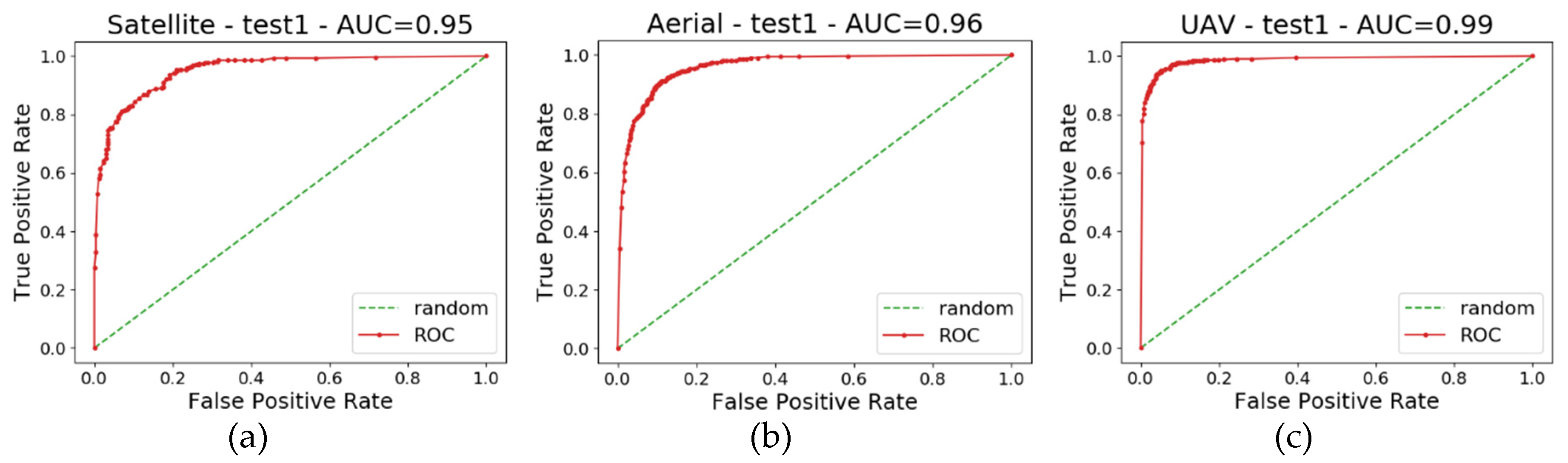
ROC (Receiver Operating Characteristic) curve and the AUC (Area Under Curve) values of test 1 in each of the resolution levels are also depicted in Figure 3. These curves show the behavior of each network with different classification thresholds and, generally, confirm the trends reported in Table 3. As expected, a progressive improvement can be noticed upon increasing the resolution of the data (i.e., UAV curves are better than satellites ones).
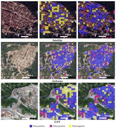
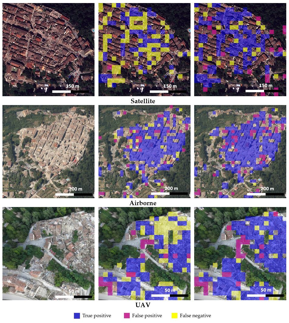
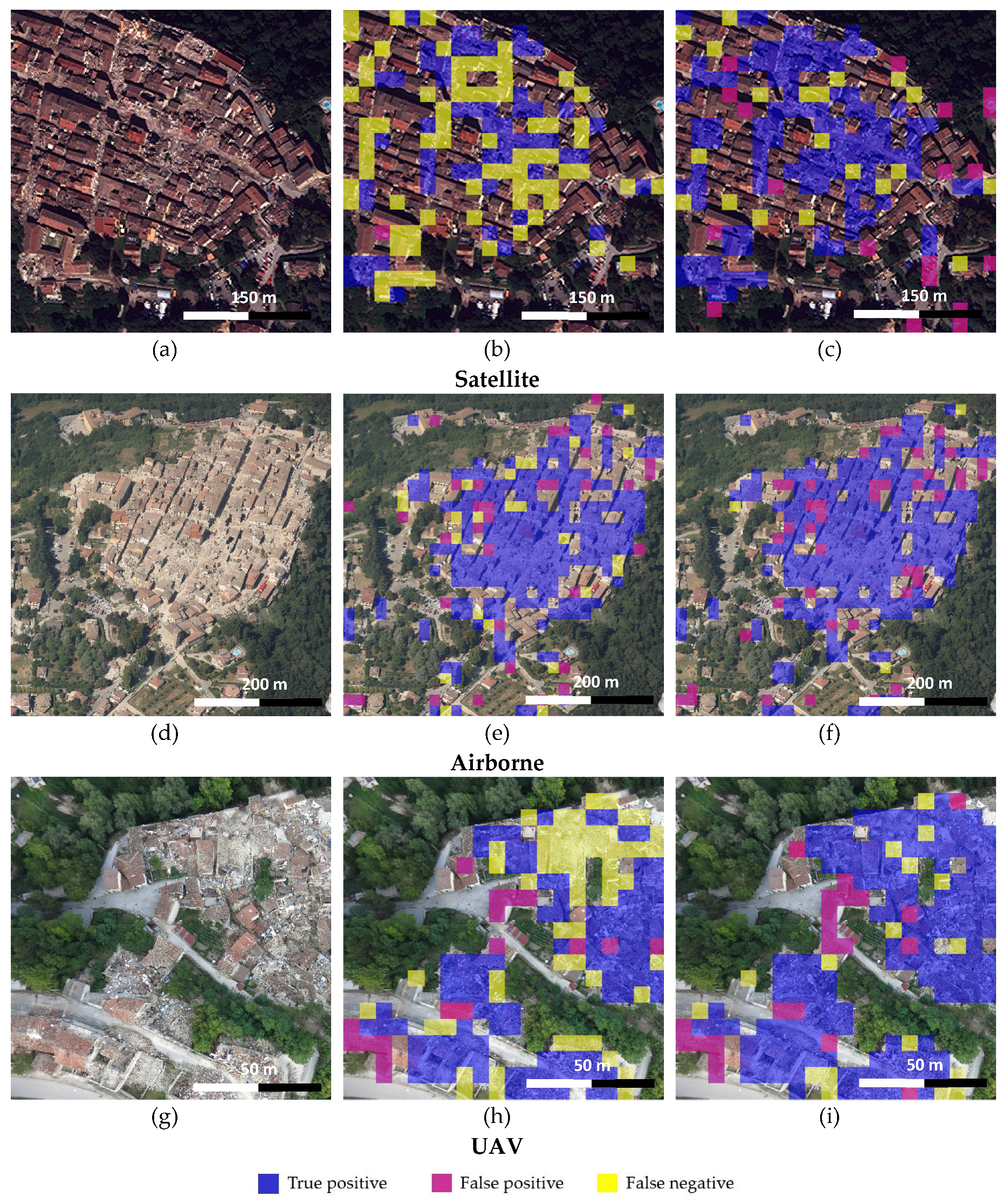
A better understanding of the classification performances and the possible failure was also given by the visual assessment of the detection results in some regions. In Figure 4, examples of a comparison between ground truth and the results achieved by the geographic transferability and the fine-tuning tests are shown. The qualitative results confirm how the fine-tuning can often complete and improve the detection of damages when the use of a pretrained network does not deliver satisfying results (i.e., in the satellite and UAV cases).
The classification task was performed on a Titan Xp GPU processor. Table 4 presents the average time needed to process a satellite, aerial and UAV image. Note that the image tiling in patches and (after the classification) the following re-composition (auxiliary operations, in Table 4) of the image overlaying building damages are not optimized in the current implementation and are still performed using CPU processing (on single core) rather than GPU processing.
6. Discussion
The presented results show that the performance using the traditional CV tests (mixing data of all the locations) yields better results in all performed tests, confirming the trends among different data resolutions presented in [15,16]. All three data categories achieve high quality metrics, with f1-scores always very close to 0.9. ROC curves are, generally, in accordance with the quality metrics and AUC is higher when platforms capturing higher resolution imagery are considered. This can be explained considering that the network can incorporate the information from all the locations and, therefore, cope with different types of data and environments. This was also the experiment that used the model with the best results on the validation dataset to determine the optimal hyperparameters for the rest of the experiments. On the other hand, the results without fine-tuning are generally worse than the other cases, as no location-specific information is given to the network. This trend was confirmed in all three data categories.
Two different aspects seem to condition the metrics in the performed tests: the variability of the image quality and the characteristics of the testing location. The first aspect is noticeable in satellite data, as each dataset was collected with different off-nadir angles and different atmospheric conditions. In this regard, the Nepal dataset suffers from an unfavorable off-nadir angle, and the presence of haze hinders easy damage detection. In this case, the building typology differences play a secondary role and can be only partially compensated by the introduction of a few training samples.
The airborne datasets returned more comparable results thanks to the lower variability in the image quality: resolution, sensor types and radiometric quality of the images are relatively similar across the datasets, and the network was able to provide more stable results. The poor quality of some datasets (e.g., Haiti slums) has a more limited effect on the achieved results. In the airborne datasets, the pre-trained model achieves higher quality metrics (e.g., f1-score) in Italian cities, thanks to the higher number of training samples from this region, showing higher performance of the model for this urban design.
The UAV datasets confirmed that the larger variability in resolution and image quality is more sensitive to the geographic location. The differences between the CV configuration and all the other tests were more evident and could only be partially compensated by fine-tuning. As in the satellite case, the network did not only have to cope with a different typology of damages, but also had to compensate for a different resolution and quality of the images.
Generally, the similarity between training samples and testing location had a direct influence on the metrics: locations with characteristics similar to the training locations provided better results than the others, as expected. In these locations, the metrics of the geographical transferability are higher. Most of the airborne datasets were acquired on Italian urban areas, with similar building characteristics—this is reflected in the higher accuracies delivered in this dataset compared to Christchurch and the Haiti slums. Hence, datasets presenting a balanced distribution among different training locations increases the capacity of the network to correctly classify new locations. This was evident in the UAV datasets, where a larger number of datasets allowed training a network to be less sensitive to the geographical area.
Fine-tuning improved the results in all the performed tests, suggesting that no overfitting of the few samples took place, even using the training loss in this process. It generated improvements that varied according to the representativeness of the training samples for the new location. A relation between the number of samples used in the fine-tuning and the corresponding improvement of the metrics is not evident. However, this improvement was very limited in the airborne dataset of Amatrice, as similar examples were present in the training samples, while being more evident in the other two test locations that significantly improved their performances by just adding few fine-tuning samples. In general, fine-tuning reduced the number of false negatives (i.e., general increase of Recall), but it often led to an over-estimation of damages (i.e., slight decrease of Precision) as confirmed by the results depicted in Figure 3. From a practical perspective, it is preferable to overestimate damages (false positives) instead of missing them (false negatives). The patch-based classification delivers faster results than pixel-based classifications, but it has the drawback of grouping all the patch pixels in the same class, often overestimating the damage extension (as shown in Figure 3), and not being able to locate and delineate damage indicators precisely within a roof or façade.
The processing time on dedicated hardware can be relatively low, as it only takes a few minutes for large images (although the sub-optimal implementation was used in the tests), and it meets the requirements of rapid mapping.
7. Conclusions and Future Developments
Recent developments in deep learning have improved traditional image analysis approaches, showing their potential in the identification of visible structural building damages. The performance of an advanced CNN for visible structural damage detection was investigated in this paper, focusing on earthquake data. In particular, the transfer learning performance at new test locations was investigated to provide some practical indications on the use of such methods in more realistic conditions compared to previous works [15,16]. The use of a small number of fine-tuning samples and the processing time needed to classify the images was also investigated to shed some light on their use in time-constrained conditions.
The presented experiments demonstrate that many elements influence the quality of the results and that it is very difficult to predict the exact behavior of the network with a dataset in advance, especially when covering different geographical areas and different building typologies with respect to the ones used as training samples. However, some general conclusions can be drawn. The achieved results show that the performance of the designed CNN is strongly related to the availability of training datasets in areas with similar typologies of damages: when the new location is similar to the training samples, the classification is reliable, as demonstrated in the Italian datasets (reaching f1-scores higher than 0.9). On the other hand, poor results were achieved for new locations that differ from the training samples. This problem was more evident when low-resolution data (i.e., satellite images) and datasets with heterogeneous quality and spatial resolutions were used: in this case, the classification was less accurate, while the adoption of fine-tuning only partially improved the results. In this regard, more standardized acquisitions, like in the airborne data, allow the training of more stable and transferable networks. Conversely, the variability of satellite and UAV data makes the quality of the results less predictable.
The performed tests highlight a gap between performances using the classical random division of samples between training and testing (i.e., CV tests), and the simulation of more realistic conditions, where no training data exist for a new location. In this regard, training using balanced datasets allows for improvement of the transferability of the network and gives more reliable solutions. All three data categories would need a more extensive training dataset with a balanced number of samples from different environments and building typologies: additional samples from regions not well represented in the current datasets (such as Nepal) would increase the reliability of the trained networks. This would lead to more reliable and stable results for any new location. The instability due to the imbalanced number of training samples could also be alleviated by introducing weights for each location according to its dataset size [49]. Fine-tuning usually improves the classification results, although it generally led to an overestimation of the damages; although this is preferable to an underestimation in an emergency context. This step, however, is highly recommendable in all the operative conditions and always leads to improvements, especially for locations not well represented in the initial training of the network. The number of fine-tuning samples to use is usually conditioned by operational constraints, but it is advisable to adopt larger sets when new urban environments are considered. From an operational perspective, this would be an important step forward with respect to the current approach as it would limit the photointerpretation effort to a subset of affected areas to fine-tune the network, instead of manually analyzing the whole area.
The presented computing times are still not fully optimized and could still be further improved with a pre-selection of the tiles to process (e.g., excluding regions corresponding to vegetation and water), as already proposed in [10]. However, the use of modern GPU processors permits classification results to be delivered quickly, considering the needs of first responders engaged in these activities, i.e., a few hours from image availability. For instance, the CEMS Rapid Mapping portfolio includes, among the post-events products, the First Estimate Product (FEP) that is “an early information product which aims at providing an extremely fast (yet rough) assessment of most affected locations within the area of interest” [50]. As the FEP should be delivered within 2 hours from the post-event image delivery, a CNN-classification with a similar processing time would be appropriate to support the activities based on photointerpretation.
The generation of reliable ground truth to train and fine-tune the network represents a critical element of the whole work, as the possible subjectivity in this step affects the reliability of the classification. For this reason, international standards on damage delineation and classification guidelines, as well as building damage scales, should be accepted and adopted by the emergency mapping community. Patch-based classification delivers rough damage identifications for quick inspection of the area, while region-based approaches (i.e., classifying separately each pixel of the image) would allow a more detailed classification at the cost of longer processing times. However, the generation of a ground truth to feed region-based classifications would also require a more detailed delineation of the damaged areas, which is often critical in high-resolution data (i.e., UAV).
The trained networks (CV tests) are now available for the community (see the Supplementary Material), as a starting point for further tests and developments. Note that the tested networks are optimized to detect structural damages caused by earthquakes or explosions, while their performance in detecting building damages produced by other types of hazard events still needs to be tested. Nevertheless, it is expected that different event types, leading to comparable structural damage evidences (e.g., roof collapse due to earthquake or wind effects) should be correctly delineated by the network regardless of the event that caused the damages used for training. On the other hand, damage types that differ substantially in appearance (e.g., burnt or flooded building, structures disintegrated or [partly] removed by tsunamis) should be properly accounted for in the training samples to be correctly detected by the network. Even in such cases, accurate damage detection will remain challenging, as described in [42]. Our investigation was also limited to the detection of damages, while actual damage assessment (in terms of damage grade classification, or identification of specific damage indicators) would require a further step that was not possible given the available data. It is also important to recall that automation of damage detection with quasi-vertical satellite data can never be as detailed and complete as mapping with multi-perspective oblique imagery. The wealth of 3D damage evidence that is often expressed quite variably among the different façades and the roof and that can be effectively mapped in aerial surveys is largely reduced to simple 2D evidence centered on the roof, with critical damage information often staying hidden and leading to substantial underestimation of damage [5]. More work will be needed on semantic processing that applies the strength of advanced machine learning to allow for detection of subtle damage proxies.
New deep learning architectures such as the most advanced domain adaptation techniques combining the use of a Generative Adversarial Network (GAN) [51] may solve the current limitations, for example, alleviating the problems caused by lack of data in the different locations. However, the potential of using these techniques in such complex and time-constrained problems still has to be explored in future research.
A recent ad-hoc training dataset tailored to emergency response activities (e.g., the public xBD satellite dataset [52], which includes over 700,000 building polygons from eight different types of natural disasters around the world, with annotated polygons and damage scores for each building) should be exploited to extend this kind of study to other natural disasters. Similar datasets would allow for not only the structural building damage detection issue to be addressed but also, damage grade assessment to be carried out at the single-building level.
The final goal would be to implement CNN-based operational tools that could be exploited by existing emergency mapping services to support and speed-up the delivery of added-value products to final users, limiting the current time-consuming photointerpretation analysis.
Supplementary Materials
The pre-trained networks using Test1 configuration are available on the following Github page: https://github.com/fnex/CNN_structural_damages.
Author Contributions
F.N. conceived the tests and drafted the paper. D.D. tested the damage assessment algorithms and supported the writing of the paper. F.G.T. and N.K. provided comments, improved the paper structure and reviewed the manuscript.
Funding
This work was partially funded by INACHUS (Technological and Methodological Solutions for Integrated Wide Area Situation Awareness and Survivor Localization to Support Search and Rescue Teams), an EU-FP7 project with grant number 607522.
Acknowledgments
The Authors would like to thank the DigitalGlobe Foundation for providing most of the satellite images used for the tests.
Conflicts of Interest
The authors declare no conflict of interest.
References
- Dell’Acqua, F.; Gamba, P. Remote Sensing and Earthquake Damage Assessment: Experiences, Limits, and Perspectives. Proc. IEEE 2012, 100, 2876–2890. [Google Scholar] [CrossRef]
- Eguchi, R.T.; Huyck, C.K.; Ghosh, S.; Adams, B.J.; McMillan, A. Utilizing New Technologies in Managing Hazards and Disasters. In Geospatial Techniques in Urban Hazard and Disaster Analysis; Springer Science and Business Media LLC: Berlin, Germany, 2009; pp. 295–323. [Google Scholar]
- United Nations INSARAG. INSARAG Guidelines, Volume II: Preparedness and Response, Manual B: Operations; United Nations INSARAG: Geneva, Switzerland, 2015. [Google Scholar]
- Voigt, S.; Giulio-Tonolo, F.; Lyons, J.; Kučera, J.; Jones, B.; Schneiderhan, T.; Platzeck, G.; Kaku, K.; Hazarika, M.K.; Czaran, L.; et al. Global trends in satellite-based emergency mapping. Science 2016, 353, 247–252. [Google Scholar] [CrossRef] [PubMed]
- Kerle, N.; Hoffman, R.R. Collaborative damage mapping for emergency response: the role of Cognitive Systems Engineering. Nat. Hazards Earth Syst. Science. 2013, 13, 97–113. [Google Scholar] [CrossRef]
- Kerle, N. Satellite-based damage mapping following the 2006 Indonesia earthquake—How accurate was it? Int. J. Appl. Earth Obs. Geoinformation 2010, 12, 466–476. [Google Scholar] [CrossRef]
- Novikov, G.; Trekin, A.; Potapov, G.; Ignatiev, V.; Burnaev, E. Satellite Imagery Analysis for Operational Damage Assessment in Emergency Situations. Business Information Systems 2018, 347–358. [Google Scholar]
- Cotrufo, S.; Sandu, C.; Tonolo, F.G.; Boccardo, P. Building damage assessment scale tailored to remote sensing vertical imagery. Eur. J. Remote. Sens. 2018, 51, 991–1005. [Google Scholar] [CrossRef]
- Gerke, M.; Kerle, N. Automatic Structural Seismic Damage Assessment with Airborne Oblique Pictometry© Imagery. Photogramm. Eng. Remote. Sens. 2011, 77, 885–898. [Google Scholar]
- Nex, F.; Duarte, D.; Steenbeek, A.; Kerle, N. Towards Real-Time Building Damage Mapping with Low-Cost UAV Solutions. Remote. Sens. 2019, 11, 287. [Google Scholar] [CrossRef]
- Lu, C.-H.; Ni, C.-F.; Chang, C.-P.; Yen, J.-Y.; Chuang, R. Coherence difference analysis of sentinel-1 SAR Interferogram to Identify Earthquake-Induced Disasters in Urban Areas. Remote. Sens. 2018, 10, 1318. [Google Scholar] [CrossRef]
- Dubois, D.; Lepage, R. Fast and Efficient Evaluation of Building Damage from Very High Resolution Optical Satellite Images. IEEE J. Sel. Top. Appl. Earth Obs. Remote. Sens. 2014, 7, 4167–4176. [Google Scholar] [CrossRef]
- Rupnik, E.; Nex, F.; Toschi, I.; Remondino, F. Contextual classification using photometry and elevation data for damage detection after an earthquake event. Eur. J. Remote Sens. 2018, 51, 543–557. [Google Scholar] [CrossRef]
- Kakooei, M. Fusion of satellite, aircraft, and UAV data for automatic disaster damage assessment. Int. J. Remote Sens. 2017, 38, 25. [Google Scholar] [CrossRef]
- Duarte, D.; Nex, F.; Kerle, N.; Vosselman, G. Multi-resolution feature fusion for image classification of building damages with convolutional neural networks. Remote Sens. 2018, 10, 1636. [Google Scholar] [CrossRef]
- Vetrivel, A.; Gerke, M.; Kerle, N.; Nex, F.; Vosselman, G. Disaster damage detection through synergistic use of deep learning and 3D point cloud features derived from very high resolution oblique aerial images, and multiple-kernel-learning. ISPRS J. Photogramm. Remote Sens. 2017, 140, 45–59. [Google Scholar] [CrossRef]
- Digitalglobe - Open data for disaster response. Available online: http://www.digitalglobe.com/ecosystem/open-data (accessed on 15 October 2019).
- OpenAerialMap. Available online: https://openaerialmap.org/ (accessed on 15 October 2019).
- Reconass - F.P.7 EU project. Available online: www.reconass.eu (accessed on 15 October 2019).
- INACHUS - F.P.7 EU Project. Available online: https://www.inachus.eu/ (accessed on 15 October 2019).
- Duarte, D.; Nex, F.; Kerle, N.; Vosselman, G. Towards a more efficient detection of earthquake induced facade damages using oblique UAV imagery. In Proceedings of the ISPRS - International Archives of the Photogrammetry, Riva del Garda, Italy, 4–7 June 2018; Remote Sensing and Spatial Information Sciences. Volume XLII-2/W6, pp. 93–100. [Google Scholar]
- Vetrivel, A.; Duarte, D.; Nex, F.; Gerke, M.; Kerle, N.; Vosselman, G. POTENTIAL OF MULTI-TEMPORAL OBLIQUE AIRBORNE IMAGERY FOR STRUCTURAL DAMAGE ASSESSMENT. ISPRS Ann. Photogramm. Remote. Sens. Spat. Inf. Sci. 2016, 355–362. [Google Scholar] [CrossRef]
- Curtis, A.; Fagan, W.F. Capturing damage assessment with a spatial video: an example of a building and street-scale analysis of tornado-related mortality in Joplin, Missouri, 2011. Ann. Assoc. Am. Geogr. 2013, 103, 1522–1538. [Google Scholar] [CrossRef]
- Ishii, M.; Goto, T.; Sugiyama, T.; Saji, H.; Abe, K. Detection of earthquake damaged areas from aerial photographs by using color and edge information. In Proceedings of the ACCV2002, Melbourne, Australia, 23–25 January 2002. [Google Scholar]
- Balz, T.; Liao, M. Building-damage detection using post-seismic high-resolution SAR satellite data. Int. J. Remote Sens. 2010, 31, 3369–3391. [Google Scholar] [CrossRef]
- Brunner, D.; Schulz, K.; Brehm, T. Building damage assessment in decimeter resolution SAR imagery: A future perspective. In Proceedings of the Joint Urban Remote Sensing Event, Munich, Germany, 11–13 April 2011; pp. 217–220. [Google Scholar]
- Armesto-González, J.; Riveiro-Rodríguez, B.; González-Aguilera, D.; Rivas-Brea, M.T. Terrestrial laser scanning intensity data applied to damage detection for historical buildings. J. Archaeol. Sci. 2010, 37, 3037–3047. [Google Scholar] [CrossRef]
- Khoshelham, K.; Oude Elberink, S.; Xu, S. Segment-based classification of damaged building roofs in aerial laser scanning data. IEEE Geosci. Remote Sens. Lett. 2013, 10, 1258–1262. [Google Scholar]
- Kerle, N.; Nex, F.; Duarte, D.; Vetrivel, A. UAV-based structural damage mapping - results from 6 years of research in two European projects. In Proceedings of the ISPRS - International Archives of the Photogrammetry, Remote Sensing and Spatial Information Sciences, Enschede, The Netherlands, 10–14 June 2019; Volume XLII-3/W8, pp. 187–194. [Google Scholar]
- Vu, T.T.; Matsuoka, M.; Yamazaki, F. Detection and animation of damage using very high-resolution Satellite Data Following the 2003 Bam, Iran, Earthquake. Earthq. Spectra 2005, 21, 319–327. [Google Scholar] [CrossRef]
- Yamazaki, F.; Vu, T.T.; Matsuoka, M. Context-based detection of post-disaster damaged buildings in urban areas from satellite images. In Proceedings of the Urban Remote Sensing Joint Event, Paris, France, 11–13 April 2007; pp. 1–5. [Google Scholar]
- Miura, H.; Yamazaki, F.; Matsuoka, M. Identification of damaged areas due to the 2006 Central Java, Indonesia earthquake using satellite optical images. In Proceedings of the Urban Remote Sensing Joint Event, Paris, France, 11–13 April 2007; pp. 1–5. [Google Scholar]
- Xu, Z.; Wu, L.; Zhang, Z. Use of active learning for earthquake damage mapping from UAV photogrammetric point clouds. Int. J. Remote Sens. 2018, 39, 5568–5595. [Google Scholar] [CrossRef]
- Li, X.; Yang, W.; Ao, T.; Li, H.; Chen, W. An improved approach of information extraction for earthquake-damaged buildings using high-resolution imagery. J. Earthq. Tsunami 2011, 5, 389–399. [Google Scholar] [CrossRef]
- Fernandez Galarreta, J.; Kerle, N.; Gerke, M. UAV-based urban structural damage assessment using object-based image analysis and semantic reasoning. Nat. Hazards Earth Syst. Sci. 2015, 15, 1087–1101. [Google Scholar] [CrossRef]
- Vetrivel, A.; Gerke, M.; Kerle, N.; Vosselman, G. Identification of damage in buildings based on gaps in 3D point clouds from very high resolution oblique airborne images. ISPRS J. Photogramm. Remote Sens. 2015, 105, 61–78. [Google Scholar] [CrossRef]
- Cusicanqui, J.; Kerle, N.; Nex, F. Usability of aerial video footage for 3D-scene reconstruction and structural damage assessment. Nat. Hazards Earth Syst. Sci. Discuss. 2018, 1–23. [Google Scholar]
- Li, Y.; Ye, S.; Bartoli, I. Semisupervised classification of hurricane damage from postevent aerial imagery using deep learning. J. Appl. Remote Sens. 2018, 12, 1–13. [Google Scholar] [CrossRef]
- Sublime, J.; Kalinicheva, E. Automatic post-disaster damage mapping using deep-learning techniques for change detection: Case Study of the Tohoku Tsunami. Remote Sens. 2019, 11, 1123. [Google Scholar] [CrossRef]
- Duarte, D.; Nex, F.; Kerle, N.; Vosselman, G. Damage detection on builiding facades using multi-temporal aerial oblique imagery. ISPRS Ann. Photogramm. Remote Sens. Spat. Inf. Sci. 2019, IV-2/W5, 8. [Google Scholar]
- Ghassemi, S.; Sandu, C.; Fiandrotti, A.; Tonolo, F.G.; Boccardo, P.; Francini, G.; Magli, E. Satellite image segmentation with deep residual architectures for time-critical applications. In Proceedings of the 26th European Signal Processing Conference (EUSIPCO), Rome, Italy, 3–7 September 2018; p. 7. [Google Scholar]
- Ghaffarian, S.; Kerle, N.; Pasolli, E.; Jokar Arsanjani, J. Post-disaster building database updating using automated deep learning: an integration of pre-disaster Openstreetmap and multi-temporal satellite data. Remote Sens. 2019, 11, 2427. [Google Scholar] [CrossRef]
- Huang, G.; Liu, Z.; van der Maaten, L.; Weinberger, K.Q. Densely Connected Convolutional Networks. In Proceedings of the 2017 IEEE Conference on Computer Vision and Pattern Recognition (CVPR), Honolulu, HI, USA, 21–26 July 2017. [Google Scholar]
- Simonyan, K.; Zisserman, A. Very deep convolutional networks for large-scale image recognition. In Proceedings of the ICLR, San Diego, CA, USA, 7–9 May 2015; pp. 1–13. [Google Scholar]
- He, K.; Zhang, X.; Ren, S.; Sun, J. Deep residual learning for image recognition. In Proceedings of the CVPR, Las Vegas, NV, USA, 26 June–1 July 2016. [Google Scholar]
- Yu, F.; Koltun, V. Multi-scale context aggregation by dilated convolutions. In Proceedings of the ICLR, San Juan, Porto Rico, 2–4 May 2016. [Google Scholar]
- Yu, F.; Koltun, V.; Funkhouser, T. Dilated residual networks. In Proceedings of the CVPR, Honolulu, HI, USA, 21–26 July 2017. [Google Scholar]
- Kingma, D.P.; Ba, J. Adam: A Method for stochastic optimization. arXiv 2014, arXiv:1412.6980. [Google Scholar]
- Buda, M.; Maki, A.; Mazurowski, M.A. A systematic study of the class imbalance problem in convolutional neural networks. Neural Netw. 2018, 106, 249–259. [Google Scholar] [CrossRef] [PubMed] [Green Version]
- CEMS Rapid Mapping. Available online: https://emergency.copernicus.eu/mapping/ems/rapid-mapping-portfolio (accessed on 10 November 2019).
- Bousmalis, K.; Silberman, N.; Dohan, D.; Erhan, D.; Krishnan, D. Unsupervised pixel-level domain adaptation with generative adversarial networks. arXiv 2017, arXiv:1612.05424. [Google Scholar]
- Gupta, R.; Goodman, B.; Patel, N.; Hosfelt, R.; Sajeev, S.; Heim, E.; Doshi, J.; Lucas, K.; Choset, H.; Gaston, M. Creating xBD: A dataset for assessing building damage from satellite imagery. In Proceedings of the The IEEE Conference on Computer Vision and Pattern Recognition (CVPR) Workshops, Los Alamitos, CA, USA, 16–20 June 2019; p. 8. [Google Scholar]
Figure 1.
Examples of building damages caused by earthquakes captured in satellite (first row), airborne (second row) and UAV (third row) images, respectively. In detail: (a) Indonesia, 2016; (b) Nepal, 2015; (c) Italy, 2009; (d) Haiti, 2010; (e) Nepal, 2015; (f) Taiwan, 2016. The damage looks different depending on the considered spatial resolution, off-nadir angle and building typology.

Figure 2.
Architecture of the network adopted in the tests: n indicates how many times the sets of convolutions composing the dense block are repeated. The dilation and the number of filters are also reported.
Figure 2.
Architecture of the network adopted in the tests: n indicates how many times the sets of convolutions composing the dense block are repeated. The dilation and the number of filters are also reported.

Figure 3.
Receiver Operating Characteristic (ROC) curves for satellite (a), airborne (b) and UAV (c) data in the CV tests. AUC values are 0.95, 0.96, 0.99 for satellite, airborne and UAV data respectively.
Figure 3.
Receiver Operating Characteristic (ROC) curves for satellite (a), airborne (b) and UAV (c) data in the CV tests. AUC values are 0.95, 0.96, 0.99 for satellite, airborne and UAV data respectively.

Figure 4.
Examples of results on different areas and resolution: (a–c) satellite (Amatrice, Italy), (d–f) airborne (Amatrice, Italy) and (g–i) UAV images (Pescara del Tronto, Italy) are depicted in three rows, respectively. Blue regions delineate the detected damages, violet, false positives and yellow, false negatives. The differences between the original image (left), geographical transferability (center) and fine-tuning tests (right) are shown.


Table 1.
Overview of the location and quantity of satellite, airborne and UAV image samples.
| Location [City (Country)] | Test ID | N. of Samples | Date [Month/Year] | Sensor/System | GSD [m] | |
|---|---|---|---|---|---|---|
| Damaged | Intact | |||||
| Satellite samples | ||||||
| L’Aquila (Italy) | S1 | 115 | 98 | April/2009 | GeoEye-1 | 0.41 |
| Port-au-Prince (Haiti) | S2 | 732 | 748 | January/2010 | GeoEye-1 | 0.41 |
| Portoviejo (Ecuador) | S3 | 47 | 85 | April/2016 | WorldView-3 | 0.31 |
| Amatrice (Italy) | S4 | 165 | 180 | August 2016 | WorldView-3 | 0.31 |
| Pesc. Tronto (Italy) | S5 | 93 | 74 | August/2016 | WorldView-3 | 0.31 |
| Kathmandu (Nepal) | S6 | 130 | 149 | April/2015 | WorldView-3 | 0.31 |
| Sukabumi (Indonesia) | S7 | 37 | 36 | January/2018 | WorldView-3 | 0.31 |
| Total | 1319 | 1370 | ||||
| Airborne samples | ||||||
| L’Aquila (Italy) | A1 | 238 | 410 | April/2009 | Pictometry | 0.10 |
| St Felice (Italy) | A2 | 337 | 301 | May/2012 | Midas | 0.10 |
| Amatrice (Italy) | A3 | 387 | 349 | September/2016 | Midas | 0.08 |
| Tempera (Italy) | A4 | 106 | 282 | April/2009 | Pictometry | 0.10 |
| Port-au-Prince (slums) (Haiti) | A5 | 409 | 293 | April/2010 | Pictometry | 0.12 |
| Port-au-Prince (Haiti) | A6 | 296 | 296 | January/2010 | Pictometry | 0.12 |
| Onna (Italy) | A7 | 242 | 142 | April/2009 | Pictometry | 0.10 |
| Christchurch (New Zealand) | A8 | 568 | 512 | April/2011 | Vexcel UCXp | 0.10 |
| Mirandola (Italy) | A9 | 143 | 141 | May/2012 | Midas | 0.10 |
| Total | 2726 | 2716 | ||||
| UAV samples | ||||||
| L’Aquila (Italy) | U1 | 74 | 241 | April/2009 | Sony ILCE-6000 | 0.02 |
| Wessel (Germany) | U2 | 70 | 73 | June/2016 | Canon EOS 600D | 0.01 |
| Portoviejo (Ecuador) | U3 | 158 | 156 | April/2016 | DJI FC300S | 0.05 |
| Pesc. Tronto (Italy) | U4 | 143 | 153 | August/2016 | Canon S110 | 0.06 |
| Kathmandu (Nepal) | U5 | 472 | 469 | April/2015 | Canon IXUS 127 | 0.05 |
| Taiwan (China) | U6 | 442 | 441 | February/2016 | DJI FC300S | 0.03 |
| Gronau (Germany) | U7 | 331 | 303 | October/2013 | Canon EOS 600D | 0.02 |
| Mirabello (Italy) | U8 | 363 | 319 | May/2012 | Olympus E-P2 | 0.02 |
| Lyon (France) | U9 | 225 | 247 | May/2017 | DJI FC330 | 0.03 |
| Roquebillière (France) | U10 | 237 | 83 | October/2018 | DJI FC330 | 0.02 |
| 2515 | 2485 | |||||
Table 2.
Performed tests for the three different data categories. The used datasets, the number of samples for training, testing and fine-tuning are also given. Experiments a are without fine-tuning, while experiments b takes advantage of fine-tuning.
Table 2.
Performed tests for the three different data categories. The used datasets, the number of samples for training, testing and fine-tuning are also given. Experiments a are without fine-tuning, while experiments b takes advantage of fine-tuning.
| Data Type | Training Datasets | Training Samples | Testing Data | Fine Tuning Samples | Testing Samples | |
|---|---|---|---|---|---|---|
| Satellite | 1 | S1,2,3,4,5,6,7 | (80%) | S1,2,3,4,5,6,7 | - | (20%) |
| 2a | S1,3,4,5,6,7 | 1209 | S2 | - | 1480 | |
| 2b | S1,3,4,5,6,7 | 1209 | S2 | 221 | 1259 | |
| 3a | S1,2,3,5,6,7 | 2344 | S4 | - | 345 | |
| 3b | S1,2,3,5,6,7 | 2344 | S4 | 90 | 255 | |
| 4a | S1,2,3,4,5,7 | 2410 | S6 | - | 279 | |
| 4b | S1,2,3,4,5,7 | 2410 | S6 | 70 | 209 | |
| 5a | S1,2,3,4,5,6 | 2616 | S7 | - | 73 | |
| 5b | S1,2,3,4,5,6 | 2616 | S7 | 24 | 49 | |
| Airborne | 1 | A1,2,3,4,5,6,7,8 | (80%) | A1,2,3,4,5,6,7,8 | - | (20%) |
| 2a | A1,2,4,5,6,7,8 | 4706 | A3 | - | 736 | |
| 2b | A1,2,4,5,6,7,8 | 4706 | A3 | 106 | 630 | |
| 3a | A,1,2,3,4,6,7,8 | 4740 | A5 | - | 702 | |
| 3b | A,1,2,3,4,6,7,8 | 4740 | A5 | 175 | 527 | |
| 4a | A,1,2,3,4,5,6,7 | 4362 | A8 | - | 1080 | |
| 4b | A,1,2,3,4,5,6,7 | 4362 | A8 | 223 | 857 | |
| UAV | 1 | U1,2,3,4,5,6,7,8,9 | (80%) | U1,2,3,4,5,6,7,8,9 | - | (20%) |
| 2a | U1,2,3,5,6,7,8,9 | 4704 | U4 | - | 296 | |
| 2b | U1,2,3,5,6,7,8,9 | 4704 | U4 | 44 | 252 | |
| 3a | U1,2,3,4,6,7,8,9 | 4059 | U5 | - | 941 | |
| 3b | U1,2,3,4,6,7,8,9 | 4059 | U5 | 188 | 753 | |
| 4a | U1,2,3,4,5,7,8,9 | 4117 | U6 | - | 883 | |
| 4b | U1,2,3,4,5,7,8,9 | 4117 | U6 | 162 | 721 |
Table 3.
Quality metrics of the performed tests. Each metric reports the average and standard deviation of the results (in brackets, only for tests 1 and b).
Table 3.
Quality metrics of the performed tests. Each metric reports the average and standard deviation of the results (in brackets, only for tests 1 and b).
| Test | Accuracy | Precision | Recall | F1-Score | |
|---|---|---|---|---|---|
| Satellite | 1 | 0.871 (±0.005) | 0.841 (±0.021) | 0.889 (±0.031) | 0.868 (±0.006) |
| 2a | 0.724 | 0.669 | 0.877 | 0.759 | |
| 2b | 0.742 (±0.006) | 0.713 (±0.016) | 0.791 (±0.034) | 0.757 (±0.008) | |
| 3a | 0.707 | 0.848 | 0.473 | 0.607 | |
| 3b | 0.784 (±0.008) | 0.774 (±0.009) | 0.775 (±0.022) | 0.774 (±0.011) | |
| 4a | 0.538 | 0.517 | 0.115 | 0.189 | |
| 4b | 0.541 (±0.01) | 0.508 (0.018) | 0.34 (±0.065) | 0.407 (±0.058) | |
| 5a | 0.877 | 0.967 | 0.784 | 0.866 | |
| 5b | 0.939 (±0.00) | 0.958 (±0.00) | 0.92 (±0.00) | 0.939 (±0.00) | |
| Airborne | 1 | 0.9 (±0.006) | 0.908 (±0.021) | 0.892 (±0.014) | 0.90 (±0.004) |
| 2a | 0.894 | 0.906 | 0.891 | 0.898 | |
| 2b | 0.91 (±0.005) | 0.903 (±0.018) | 0.949 (±0.021) | 0.919 (±0.005) | |
| 3a | 0.719 | 0.702 | 0.902 | 0.789 | |
| 3b | 0.786 (±0.008) | 0.774 (±0.014) | 0.9 (±0.037) | 0.83 (0.010) | |
| 4a | 0.807 | 0.909 | 0.706 | 0.795 | |
| 4b | 0.852 (±0.008) | 0.887 (±0.023) | 0.824 (±0.025) | 0.85 (±0.008) | |
| UAV | 1 | 0.931 (±0.007) | 0.947 (±0.004) | 0.921 (±0.013) | 0.931 (±0.008) |
| 2a | 0.825 | 0.934 | 0.692 | 0.795 | |
| 2b | 0.861 (±0.025) | 0.933 (±0.012) | 0.754 (±0.057) | 0.84 (±0.035) | |
| 3a | 0.674 | 0.741 | 0.538 | 0.623 | |
| 3b | 0.752 (±0.044) | 0.803 (±0.017) | 0.651 (±0.105) | 0.725 (±0.071) | |
| 4a | 0.828 | 0.837 | 0.814 | 0.826 | |
| 4b | 0.908 (±0.011) | 0.859 (±0.040) | 0.969 (±0.031) | 0.915 (±0.007) |
Table 4.
Processing time for satellite, aerial and UAV. The satellite case shows the processing time for an image of 15,200 × 10,400 pixel. The aerial case shows the processing time an image of 5616 × 3744 pixel. The UAV case shows the processing time of an image of 4000 × 3000 pixel.
Table 4.
Processing time for satellite, aerial and UAV. The satellite case shows the processing time for an image of 15,200 × 10,400 pixel. The aerial case shows the processing time an image of 5616 × 3744 pixel. The UAV case shows the processing time of an image of 4000 × 3000 pixel.
| Prediction | Auxiliary Operations | Total | |
|---|---|---|---|
| Satellite | 19 min | 5 min | 24 min |
| Aerial | 53 s | 6 s | 1 min |
| UAV | 15 s | 4 s | 19 s |
© 2019 by the authors. Licensee MDPI, Basel, Switzerland. This article is an open access article distributed under the terms and conditions of the Creative Commons Attribution (CC BY) license (http://creativecommons.org/licenses/by/4.0/).
Share and Cite
MDPI and ACS Style
Nex, F.; Duarte, D.; Tonolo, F.G.; Kerle, N. Structural Building Damage Detection with Deep Learning: Assessment of a State-of-the-Art CNN in Operational Conditions. Remote Sens. 2019, 11, 2765. https://doi.org/10.3390/rs11232765
AMA Style
Nex F, Duarte D, Tonolo FG, Kerle N. Structural Building Damage Detection with Deep Learning: Assessment of a State-of-the-Art CNN in Operational Conditions. Remote Sensing. 2019; 11(23):2765. https://doi.org/10.3390/rs11232765
Chicago/Turabian StyleNex, Francesco, Diogo Duarte, Fabio Giulio Tonolo, and Norman Kerle. 2019. "Structural Building Damage Detection with Deep Learning: Assessment of a State-of-the-Art CNN in Operational Conditions" Remote Sensing 11, no. 23: 2765. https://doi.org/10.3390/rs11232765
Note that from the first issue of 2016, this journal uses article numbers instead of page numbers. See further details here.