The Optimal Threshold and Vegetation Index Time Series for Retrieving Crop Phenology Based on a Modified Dynamic Threshold Method

Abstract

Crop phenology is an important parameter for crop growth monitoring, yield prediction, and growth simulation. The dynamic threshold method is widely used to retrieve vegetation phenology from remotely sensed vegetation index time series. However, crop growth is not only driven by natural conditions, but also modified through field management activities. Complicated planting patterns, such as multiple cropping, makes the vegetation index dynamics less symmetrical. These impacts are not considered in current approaches for crop phenology retrieval based on the dynamic threshold method. Thus, this paper aimed to (1) investigate the optimal thresholds for retrieving the start of the season (SOS) and the end of the season (EOS) of different crops, and (2) compare the performances of the Normalized Difference Vegetation Index (NDVI) and Enhanced Vegetation Index (EVI) in retrieving crop phenology with a modified version of the dynamic threshold method. The reference data included SOS and EOS ground observations of three major crop types in 2015 and 2016, which includes rice, wheat, and maize. Results show that (1) the modification of the original method ensures a 100% retrieval rate, which was not guaranteed using the original method. The modified dynamic threshold method is more suitable to retrieve crop SOS/EOS because it considers the asymmetry of crop vegetation index time series. (2) It is inappropriate to retrieve SOS and EOS with the same threshold for all crops, and the commonly used 20% or 50% thresholds are not the optimal thresholds for all crops. (3) For single and late rice, the accuracies of the SOS estimations based on EVI are generally higher compared to those based on NDVI. However, for spring maize and summer maize, results based on NDVI give higher accuracies. In terms of EOS, for early rice and summer maize, estimates based on EVI result in higher accuracies, but, for late rice and winter wheat, results based on NDVI are closer to the ground records.

1. Introduction

Crop phenology refers to seasonal and recurring crop developments, such as emergence, greening, jointing, heading, grouting, maturity, and more [1]. Crop phenological information is of great importance for agricultural production management and decision-making [2,3]. It is also an important parameter for crop growth monitoring, yield prediction, and crop growth modeling using process-driven models [4]. Information about phenology provides important parameters to extract the crop planting area and the crops’ response to climate change [5,6].

Agro-ecosystems are ecosystems that are strongly affected by natural conditions and human activities [7]. Therefore, any changes in crop phenology are closely related to climate change and human activities, which makes it an important indicator of changes in terrestrial systems. Accurate retrieval of crop phenology information also contributes to scientific research in global climate change, global carbon balance, ecological processes evolution, and more [8].

Currently, crop phenological information is mainly derived through three methods.

(1) Ground observation. Ground observations depend on direct human observations and can be considered reference data. Specialists, as well as interested volunteers (citizen science), record crop growth and development information at the field level. The advantages of direct observations are rooted in their simplicity, high precision, and long-time span [9,10]. However, this method is labor-intensive and only a limited number of observation stations exist providing continuous observations. Moreover, the relatively small coverage and uneven spatial distribution of networks make it difficult to monitor crop phenology at a large scale with fine spatial resolution [11].

(2) Retrieval from web camera networks. More recently, near-surface remote sensing techniques have been developed to monitor the growth and development of vegetation at canopy to landscape levels [12]. In the United States, for example, the PhenoCam network has been constructed based on high-resolution digital cameras at more than 200 sites. The network generates continuous high spatial and temporal resolution imagery and allows analysis of vegetation phenological information with high accuracy [13,14,15]. Despite its merits, the limited monitoring scope makes it difficult to be applied at continental or global scales.

(3) Retrieval from satellite time-series data. Satellite remote sensing technology has been investigated and practiced successfully in retrieving vegetation phenology based on remotely sensed vegetation index (VI) time-series data at large scales [16,17]. Vegetation index time series are good indicators reflecting the dynamics of vegetation growth and vegetation coverage, such as the Normalized Difference Vegetation Index (NDVI) and the Enhanced Vegetation Index (EVI). These two simple indices have become the most commonly used data sources for retrieving vegetation phenology. Up to now, the most important and well-studied phenological parameters include the start of the season (SOS), the end of the season (EOS), and the peak of the season (PS) [18,19]. The advantage of this method is that vegetation phenological information can be continuously monitored at regional to global scales. Suitable data sets the date back to the 1980s. On the downside, it must be noted that the earth observation (EO) derived indicators do not directly infer crop development stages (in sensu stricto), but are, instead, monitoring crop growth, which is not always closely linked to key developmental events [20]. For this reason, the scientific community generally refers to LSP (land surface phenology) when EO-based techniques are used [21].

On an operational basis, global phenological information is currently produced from MODerate-resolution Imaging Spectroradiometer (MODIS) observations within the global land cover dynamics product (MLCD) issued by the National Aeronautics and Space Administration of the United States (NASA) [22]. However, input data quality and retrieval methods lead to uncertainties in this product, and its accuracy remains to be validated globally.

Among all vegetation phenological parameters, the start of the season (SOS) and the end of the season (EOS) are the most important. Other parameters such as length of season etc. are derived from SOS and EOS [23]. At present, a variety of methods have been developed to extract vegetation phenological parameters from vegetation index time series, including the fixed threshold method [24,25], the dynamic threshold method [26,27], the moving average method [28,29], the function fitting method [30,31], the maximum-slope method [32], and the valley detection method [16,33]. Among these methods, key advantages of the dynamic threshold method are that less parameters are needed, while the method eases applicability and guarantees high accuracy. For those reasons, the dynamic threshold method is among the most commonly used methods for retrieving vegetation SOS and EOS.

When using the dynamic threshold method, many studies use either the 20% threshold [34,35,36] or the 50% threshold [10,19,37]. Currently, most studies on crop phenology research use the same thresholds across various crops and geographies. For example, Ren et al. [18] used the 20% threshold to retrieve wheat SOS and EOS in the major wheat growing regions of the world. In their study, they used EVI time series data from 1981 to 2014 and studied their responses to climate change at a global scale. Guo et al. [38] used NDVI time series from 1993 to 2008 to retrieve the SOS of winter wheat in China with the 20% threshold. The study also compared spatio-temporal trends based on ground observations and remote sensing data. Alcantara et al. [39] used the dynamic threshold method to extract land surface phenology (including SOS and EOS with 20% threshold). It was found that phenology metrics can help map abandoned agriculture. Wu et al. [40] used NDVI time series to retrieve both the start and end of the season dates for crops in China with the 20% threshold, and then analyzed the spatial pattern of cultivated land phenology in China.

Clearly, compared to natural vegetation, crop growth is not only driven by natural (climate) conditions, but also modified through field management activities [5,41]. Hence, anthropogenic influences have to be considered. Moreover, multiple growth cycles can be completed during one calendar year [42,43]. This may lead to complicated planting patterns and interfering growth patterns within mixed pixels. Taking China as an example, there are not only different cropping cycles such as single cropping, double cropping, and triple cropping, but, at the same time, different crop rotations and varied intercropping practices. Therefore, it is far more difficult to retrieve crop phenology in agricultural systems compared to less human-impacted ecosystems. Unmixing approaches have been proposed to decouple the mixed signal of several crops within mixed pixels, but have their own limitations [44].

Although a large number of studies have used the dynamic threshold method to extract crop phenological parameters, there are relatively few studies focusing on the following questions.

• Are the commonly used 20% or 50% thresholds suitable for retrieving crop SOS and EOS?
• Is it feasible to use the same threshold to retrieve SOS and EOS in cropland with multiple cropping, since the time series of VIs of each growing season are always asymmetrical?
• Are there index-specific differences between the LSP parameters retrieved from NDVI and EVI time series?

To fill this research gap, this paper attempted to identify the most suitable vegetation index time series for retrieving crop phenology based on a modified dynamic threshold method and to evaluate which threshold is optimal. Decisions were taken based on a comparison against ground observations as a reference. We first defined SOS and EOS dates of three major crops (rice, wheat, and maize) from 2015 to 2016 using ground records. Then, for the same period, smoothed and gap-filled MODIS NDVI and EVI time series were calculated. Based on the pre-processed time series, the dynamic threshold method was modified to ensure a 100% retrieval rate. Then the improved dynamic threshold method was used to retrieve crop SOS and EOS from NDVI and EVI time series with different thresholds. Lastly, the crop-specific optimal thresholds for retrieving SOS and EOS and the performances of NDVI and EVI were evaluated.

2. Data

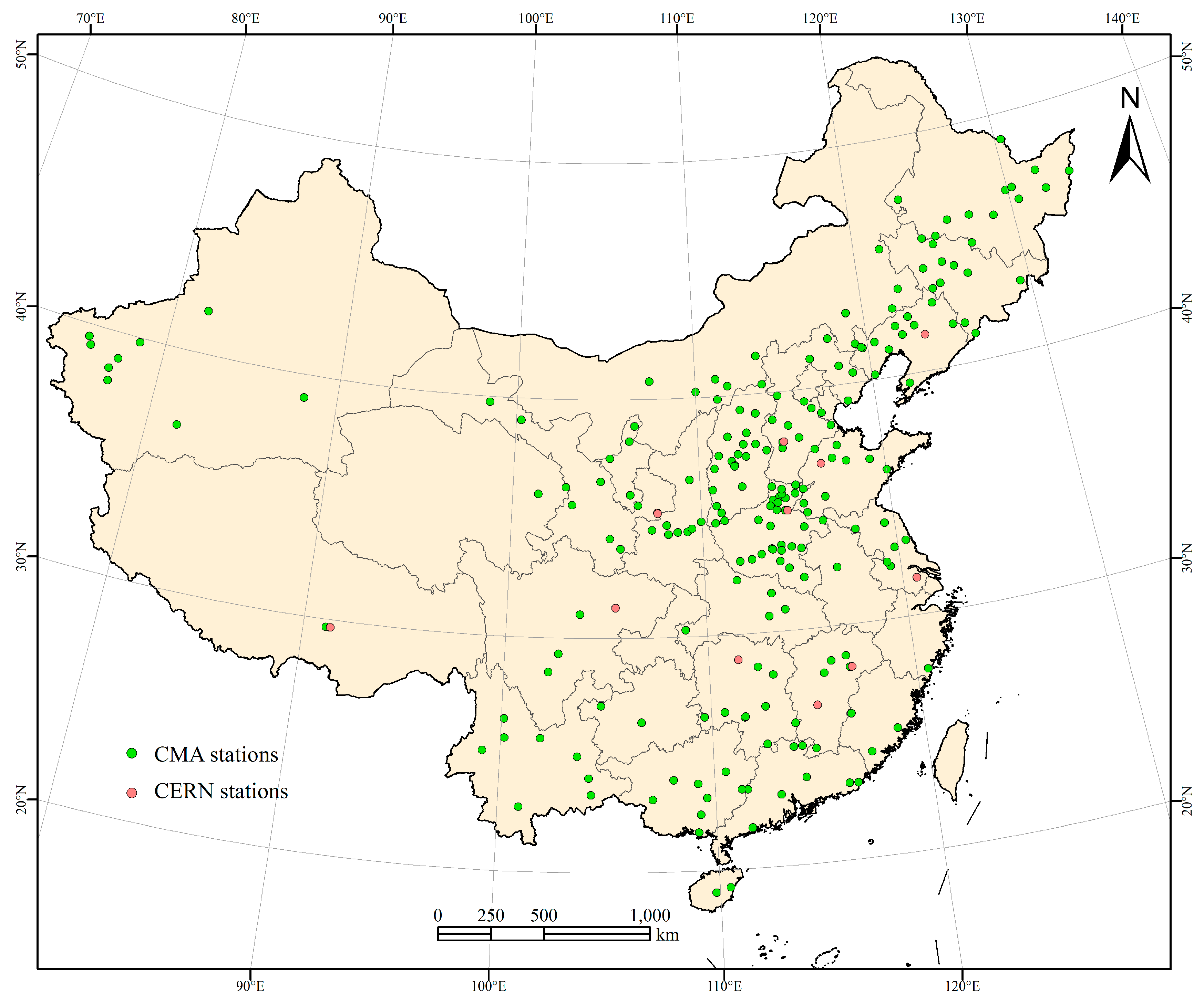
2.1. Ground Observation Data

The ground observation data were derived from the China Meteorological Administration (CMA) and the Chinese Ecosystem Research Network (CERN). The data from CMA contains the field records of crop growth and development status observed by China’s agrometeorological stations since September 1991. The specific contents include, among others, crop name, the name of the crop development stage and its date, the anomaly of the development stage, and the degree of the development stage. Supported by the Chinese Academy of Sciences, CERN was established in 1988 to monitor water, soil, atmosphere, biology, energy flow, and other important ecological processes of various ecosystems in China under unified rules. It consists of 16 agriculture ecosystem stations, 11 forest ecosystem stations, three grassland ecosystem stations, and seven desert, ocean, lake, swamp, and urban ecosystem stations and research centers. The ground observation data used in this paper were from CERN farmland ecosystem stations.

The CMA data recorded the detailed phenological period of crops, including rice, wheat, maize, cotton, rapeseed, and more. The CERN data recorded the major phenological periods of crops, including rice, wheat, maize, etc. For rice and wheat, the recorded green-up dates were selected as a proxy to evaluate SOS retrieval accuracy. However, for maize, only the three-leaf date records were relatively complete. Observations of the five-leaf date and the seven-leaf date were inconsistent. Therefore, we had to use the three-leaf date to evaluate the retrieved SOS of maize. To evaluate the accuracy of the retrieved EOS, the maturity date of each crop was selected. To ensure that there were enough observations as reference data, both records from CMA and CERN in 2015 and 2016 were jointly used. Averaged dates were calculated and used for stations with multiple records of the same crop. However, since the CERN data did not record maize three-leaf date, the reference data for assessing maize SOS were only from CMA records.

The spatial distribution of the observation stations is shown in Figure 1 and the number of available observation data for each crop is shown in

Table 1. Number of available reference data for each crop.

Crop Types	Cropping Types	Number of SOS Reference Data	Number of EOS Reference Data
Single rice	Single cropping	16	35
Early rice	First crop in double cropping	11	10
Late rice	Second crop in double cropping	13	15
Winter wheat	First crop in double cropping	36	36
Spring maize	Single cropping	47	54
Summer maize	Second crop in double cropping	25	34

. Note that observations in areas with strong noise in the VI time series were excluded to ensure the representativeness and quality of the field reference samples.

2.2. Remote Sensing Data

Remote sensing data were downloaded from the Land Processes Distributed Active Archive Center (LP DAAC) website (https://lpdaac.usgs.gov/), including the MOD09A1 and MOD09Q1 products from 2015 to 2016. The time resolution of both products is eight days. The spatial resolution of MOD09A1 is 500 meters. It contains reflectance data of seven bands. The spatial resolution of MOD09Q1 is 250 meters, only containing red and near-infrared reflectance bands.

NDVI time series at 250 m spatial resolution was calculated using the red and near-infrared bands from the MOD09Q1 (Equation (1)). To compute EVI (Equation (2)), the blue band from MOD09A1 was resampled to 250 meters using the bilinear interpolation.

$$NDVI=\frac{{\rho }_{NIR}-{\rho }_R}{{\rho }_{NIR}+{\rho }_R}$$

(1)

$$EVI=\frac{2.5\left({\rho }_{NIR}-{\rho }_R\right)}{{\rho }_{NIR}+6.0{\rho }_R-7.5{\rho }_B+1}$$

(2)

where ${\rho }_{NIR}$, ${\rho }_R$, and ${\rho }_B$ represent the reflectance of the near-infrared, red, and blue bands, respectively.

Although MOD09A1 and MOD09Q1 products contain the best observations within the eight-day compositing periods to eliminate the effects of clouds and the atmosphere, noise in the data has not been completely eliminated. To remove the remaining noise and to smooth the curves, the NDVI and EVI time series were filtered before retrieving crop SOS and EOS [45]. First, noisy observations in NDVI and EVI were detected according to the quality file contained in the products. Data with poor quality were substituted with the linear interpolation of its predecessor and successor. After that, the synthesized time-series data was filtered by Changing-Weight Filtering (CW) [46]. Only the processed NDVI and EVI time series were used for a subsequent calculation and analysis.

3. Methods

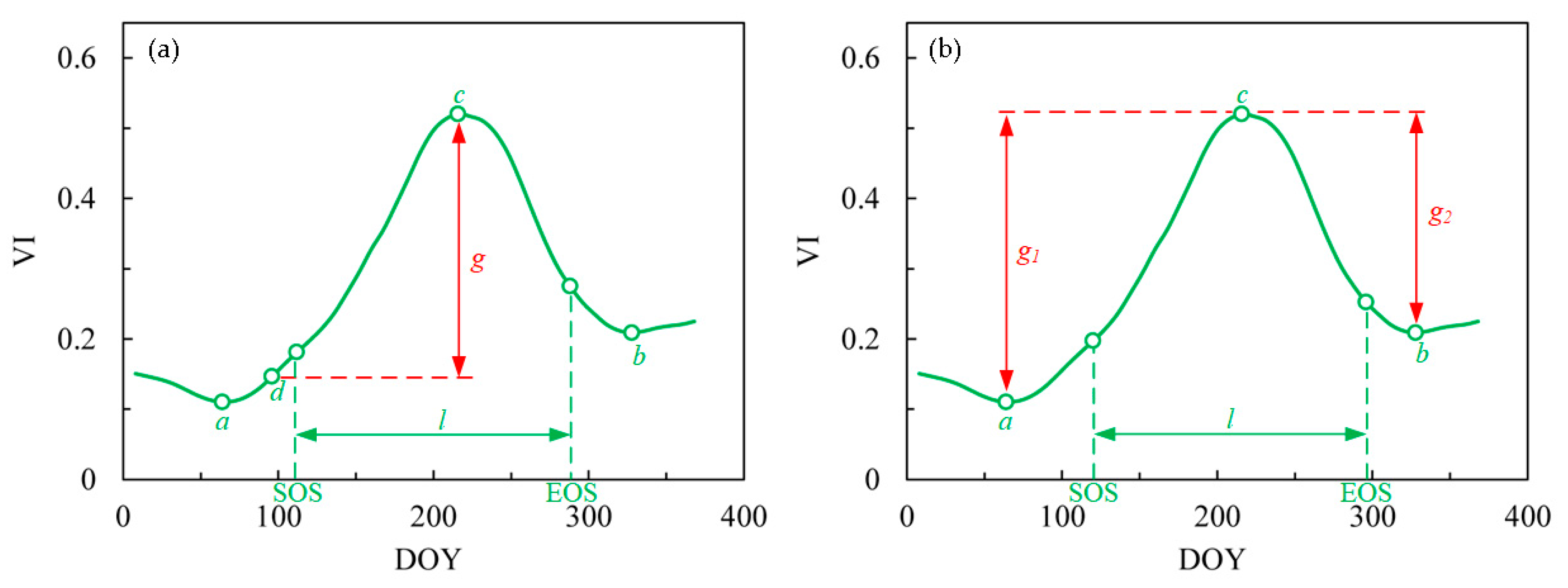
3.1. The Dynamic Threshold Method

The dynamic threshold method was first proposed by White et al. [27]. The method is also known as the local threshold method. The approach was further developed by Jönsson et al. [26,47] and implemented into TIMESAT software.

A diagrammatic sketch of the original method is shown in Figure 2a, where c is the maximum VI value within the growing season, a is the minimum VI value on the left side of c, b is the minimum value on the right side of c, and d is the average of the left minimum and the right minimum.

In the original method, the amplitude of the growing season (g) is defined as the difference between c and d. Usually, a user-defined amplitude threshold $V{I}_{thd}$ is preset (e.g., 20%). SOS is then defined as the first date that the corresponding VI is greater than $a+V{I}_{thd}\ast g$ on the left side, and EOS is defined as the first date that the corresponding VI is smaller than $b+V{I}_{thd}\ast g$ on the right side of the maximum. The formula is shown in Equation (3).

$$\left\{\begin{array}{c}V{I}_{SOS}\ge a+V{I}_{thd}\ast g\\ V{I}_{EOS}\le b+V{I}_{thd}\ast g\end{array}\right\}$$

(3)

Since VI index time series of crops tend to be highly asymmetrical, especially when multiple growing seasons are present, the use of Equation (3) often fails to obtain reliable SOS or EOS, especially when a large difference between the left (a) and the right minimum (b) exists. On the side with the higher minimum, the retrieval of SOS or EOS is likely to fail. Therefore, $a+V{I}_{thd}\ast g$ or $b+V{I}_{thd}\ast g$ will be greater than the maximum VI (c). This will inevitably lead to the failure of detecting a corresponding VI value, and make it impossible to obtain correct SOS or EOS values.

To solve this problem, this paper improved the dynamic threshold method.

We canceled the base value (d) and instead propose using two different amplitudes when retrieving SOS and EOS (g₁ and g₂, Figure 2b). The amplitude used in the retrieval of SOS is the difference between c and the minimum VI value on the left side (a), as shown by g₁ in Figure 2b. Correspondingly, the amplitude used in retrieving EOS is the VI maximum value of the growing season (c) minus the VI minimum value of the right side (b), as shown by g₂. The calculations of SOS and EOS thresholds are summarized in Equation (4).

$$\left\{\begin{array}{c}V{I}_{SOS}\ge a+V{I}_{thd}\ast g_1\\ V{I}_{EOS}\le b+V{I}_{thd}\ast g_2\end{array}\right\}$$

(4)

The modification ensures that the following conditions are always met: $V{I}_{thd}$ ≤ 100%, $V{I}_{SOS}$ ≤ c and $V{I}_{EOS}$ ≤ c. This guarantees that the modified algorithm always finds the corresponding $V{I}_{SOS}$ and $V{I}_{EOS}$. Therefore, the failure in retrieving SOS or EOS can be avoided.

3.2. Validation of the Improved Dynamic Threshold Method

To evaluate the applicability of the improved method, we introduced the success rate B. As shown in Equation (5), the larger the B value, the higher the number of successful retrievals.

$$B=\frac{m}{M}\times 100\%$$

(5)

In the formula, $m$ is the sum of the growing season number of samples whose SOS or EOS can be successfully retrieved, and $M$ is the sum of the growing season number of all samples.

3.3. Accuracy Assessment of the Retrieved Phenology

Three indicators were used to evaluate the accuracy of the retrieved phenological parameters with respect to the reference measurements [42,48] Equations (6)–(8): Coefficient of determination (R²), Root Mean Square Error (RMSE), and BIAS. R² reflects the consistency and linear correlation between the retrieved SOS or EOS and the reference data. The closer the R² is to 1, the higher the consistency between them. RMSE is the average error between the retrieved results and the reference data measured along the 1:1 line. A smaller RMSE means a higher accuracy of the retrieved result. BIAS is defined as the number of days that the retrieved SOSs or EOSs deviate from the ground observations. A smaller absolute value of BIAS indicates a higher accuracy of the retrieved results.

$$R^2=\frac{cov{\left(\widehat{Y},Y\right)}^2}{var\left(\widehat{Y}\right)var\left(Y\right)}$$

(6)

$$RMSE=\sqrt{\frac{{{\displaystyle \sum }}_{i=1}^N{({\widehat{Y}}_i-Y_i)}^2}{N}}$$

(7)

$$BIAS=\frac{{{\displaystyle \sum }}_{i=1}^N({\widehat{Y}}_i-Y_i)}{N}$$

(8)

In Equations (6)–(8), ${\widehat{Y}}_i$ is the retrieved SOS or EOS of the $i$ th sample, and $Y_i$ is the corresponding reference SOS or EOS. $N$ is the number of samples. If ${\widehat{Y}}_i-Y_i$ is greater than 0, it will be recorded as 1, and if ${\widehat{Y}}_i-Y_i$ is smaller than 0, it will record as -1. $cov(\widehat{Y},Y)$ represents the covariance between the retrieved phenology and the reference phenology. $Var(\widehat{Y})$ and $Var\left(Y\right)$ represent the variance of the retrieved phenology and the reference phenology, respectively.

4. Results

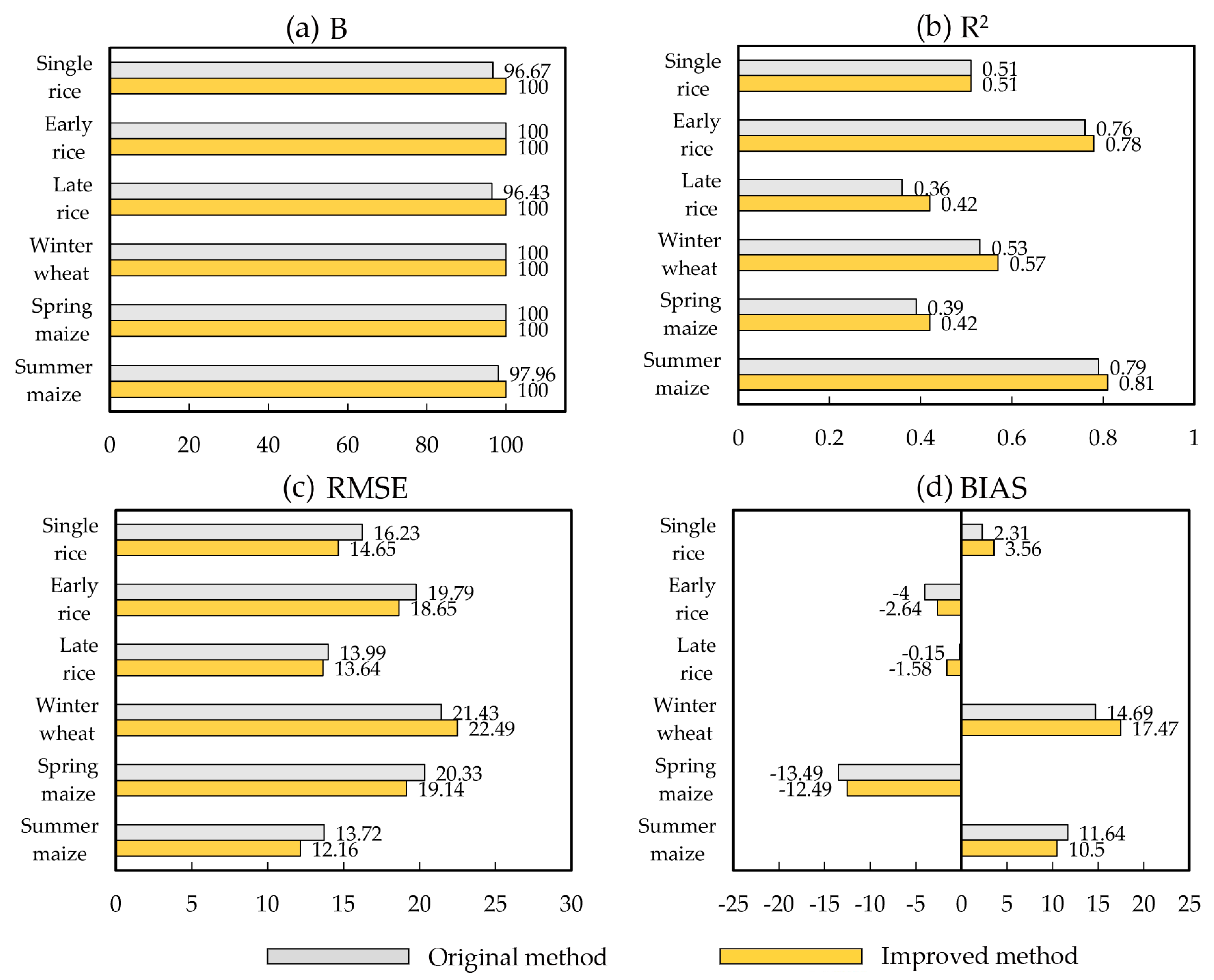
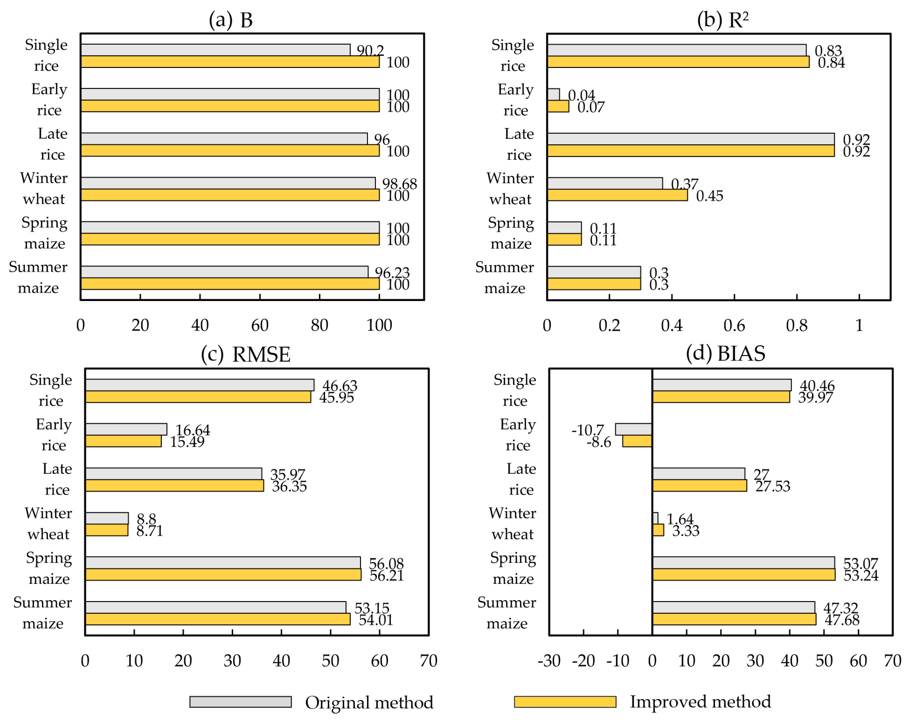
4.1. Comparison of the Original and the Improved Dynamic Threshold Method

As a baseline, we used the 20% amplitude threshold to retrieve crop SOS and EOS based on MODIS NDVI time series. When evaluating the performance of the improved method (e.g., when calculating the success rate B of retrieval results), we counted all samples. However, when calculating the accuracies of the estimates against the field observations, we only use those samples that were successfully retrieved by the original method. In this way, the samples used to evaluate the retrieval accuracies of the two methods are identical. It ensures the comparability of the two methods. The retrieval results before and after the modifications of the algorithm are shown in Figure 3 and Figure 4, respectively. The success rate of crop SOS and EOS of the original approach (e.g., before improvement) is between 90% and 100%. After the modification, SOS and EOS of all samples can be successfully retrieved. This improvement can be particularly well seen for crops with complex background conditions such as single rice and double rice. For single rice, the success rate of SOS increased from 96.7% to 100%, and the successful retrieval rate of EOS increase from 90.2% to 100%. For other crops, the success rate of SOS and EOS are also improved to some extent. In addition, for most crops, the retrieval accuracy of SOS and EOS slightly improves. The RMSE of the retrieved SOS of early rice decreases from 19.8 to 18.7 days, and the RMSE of its retrieved EOS decreases from 16.6 to 15.5 days.

For most crops, the differences between BIAS of the retrieved SOS and EOS are large. For winter wheat, the BIAS of SOS is 17.5 days. In addition, for spring maize, the BIAS of EOS is 53.1 days. This indicates that the 20% threshold is not the optimal threshold for retrieving SOS and EOS of all crops, and there is still room for accuracy improvement. Moreover, it is inappropriate to use the same threshold to retrieve SOS and EOS for crops. For example, the retrieval accuracy based on the 20% threshold of late rice SOS is comparatively higher than that of EOS. Based on a 20% threshold, the RMSE of the retrieved SOS of late rice is 13.6 days, but the RMSE of the retrieved EOS of late rice is 36.4 days. To improve the retrieval accuracy, it is recommended to use different thresholds to retrieve SOS and EOS for the same crop.

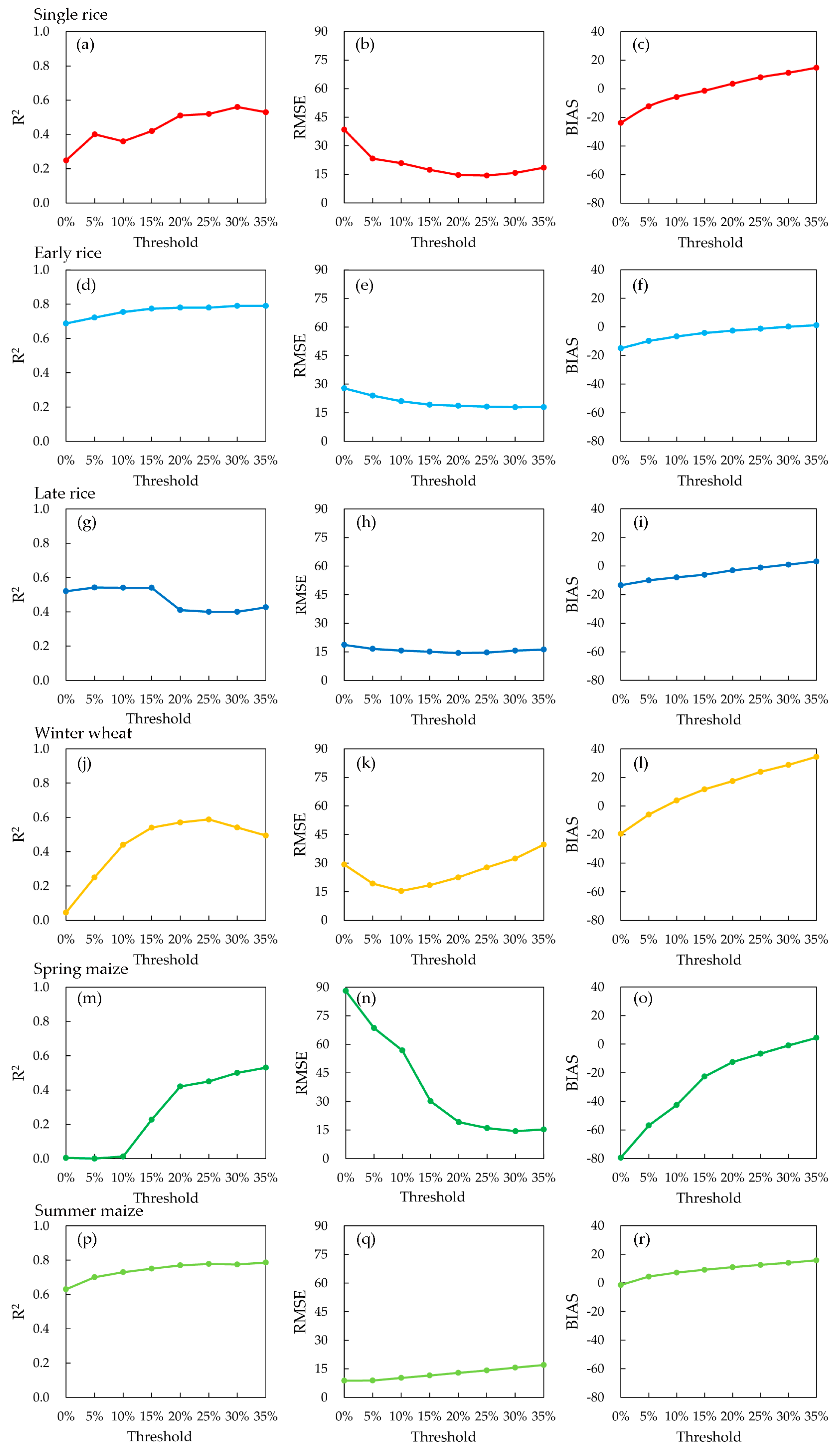
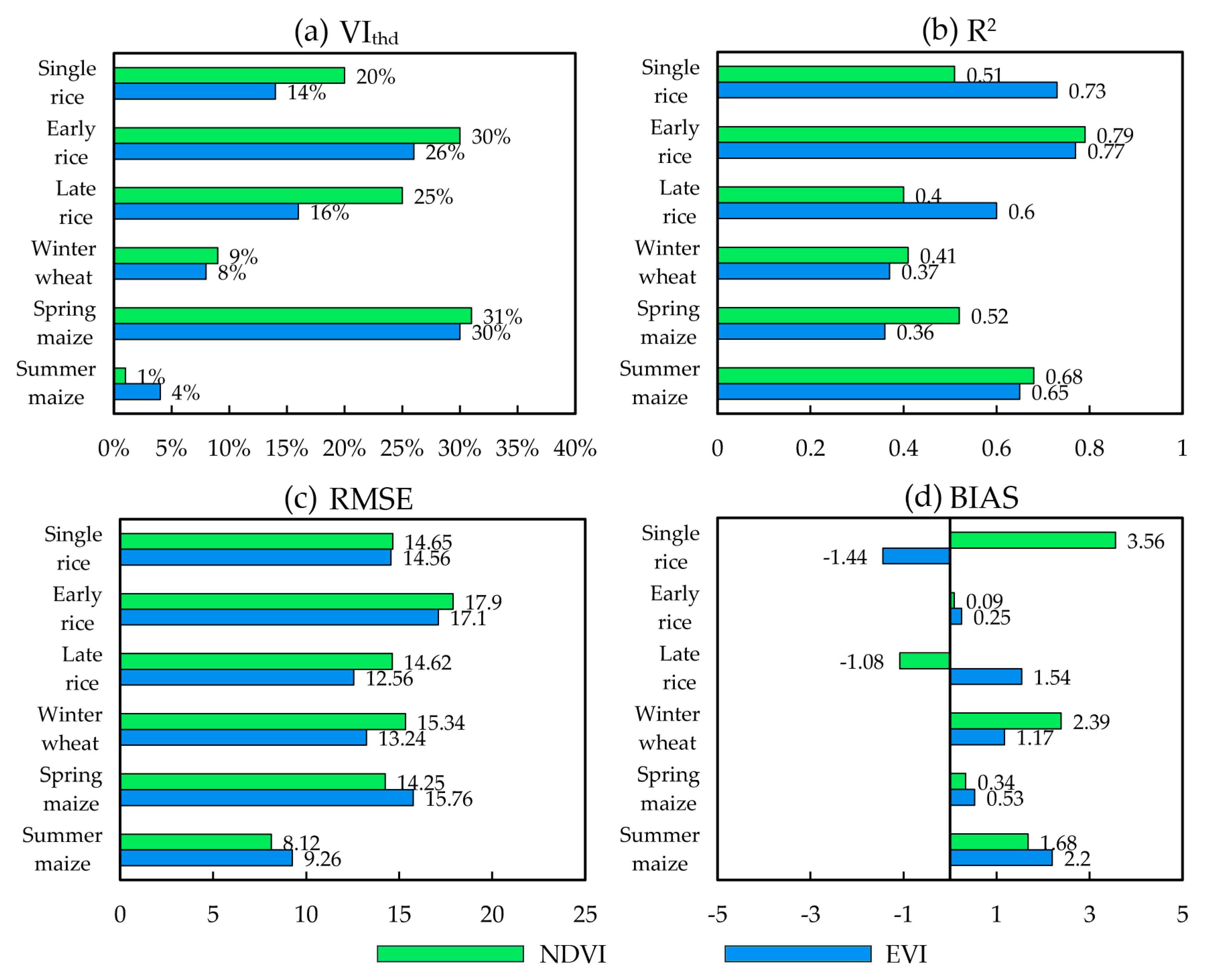
4.2. The Optimal Thresholds for Retrieving SOS

To determine the crop-specific optimum thresholds for SOS retrievals, we gradually adjust the threshold by steps of 5% from 0% to 35% for each of the crops. The retrieved SOS based on MODIS NDVI time series was then used to calculate the accuracy of the retrieved SOS under different thresholds (Figure 5). For all crops, as the threshold gradually increases, the values of BIAS decrease toward a minimum before increasing again. Except late rice, the values of R² increase as the threshold increases. As for single rice, early rice and spring maize, their RMSE decrease as the threshold increases. However, for winter wheat and summer maize, their RMSE increase as the threshold increases. Therefore, for single rice and late rice, the optimal threshold to retrieve SOS is 20% and 25%, respectively. For early rice and spring maize, the optimal threshold is approximately 30%, while, for summer maize and winter wheat, the optimal thresholds are around 10%.

The most suitable threshold interval was further fine-tuned in steps of 1% to detect the optimal threshold. The optimal threshold for retrieving SOS of each crop is shown in

Table 2. Crop-specific optimal thresholds for retrieving the start of the season (SOS) based on Normalized Difference Vegetation Index (NDVI).

Crop Types	$\mathbf{Number} \mathbf{of} \mathbf{Samples}$	$\mathit{V}{\mathit{I}}_{\mathit{t}\mathit{h}\mathit{d}}$	R2	RMSE (DAYS)	BIAS (DAYS)
Single rice	16	20%	0.51	14.7	3.6
Early rice	11	30%	0.79	17.9	0.1
Late rice	13	25%	0.40	14.6	−1.1
Winter wheat	36	9%	0.41	15.3	2.4
Spring maize	47	31%	0.52	14.3	0.3
Summer maize	25	1%	0.68	8.1	1.7

. Among the six crops, the optimal threshold of spring maize and early rice are the highest at 31% and 30%, respectively. The optimal threshold of summer maize and winter wheat are the lowest at 1% and 9%, respectively. The optimal threshold of single rice and late rice are 20% and 25%, respectively. Among the different crops, the accuracy of the retrieved SOS of summer maize is the highest, with R² of 0.68, RMSE of 8.1 days, and BIAS of 1.7 days. On the contrary, the accuracy of the retrieved SOS of early rice is the lowest, with R² of 0.79, RMSE of 17.9 days, and BIAS of 0.1 days.

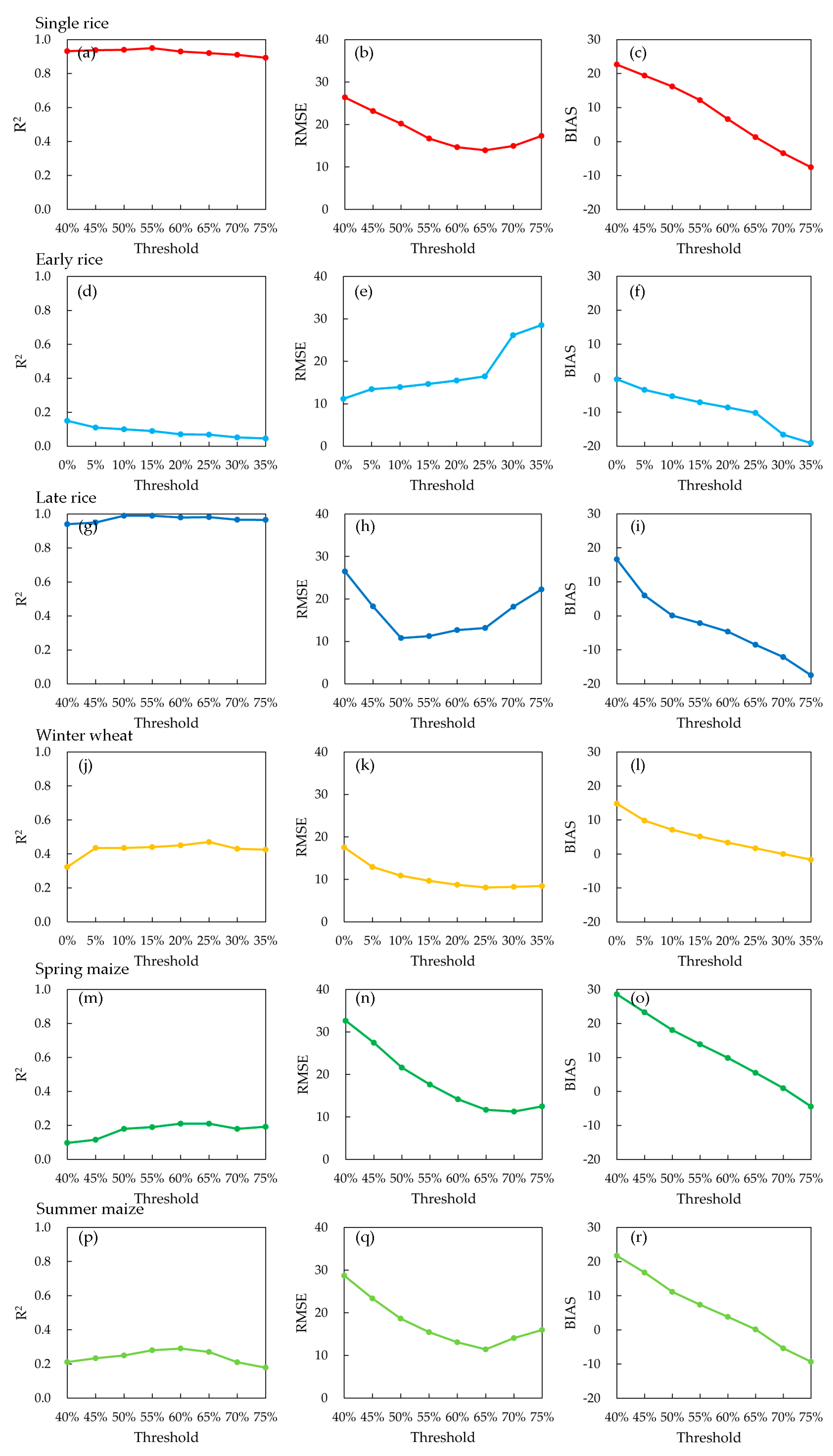
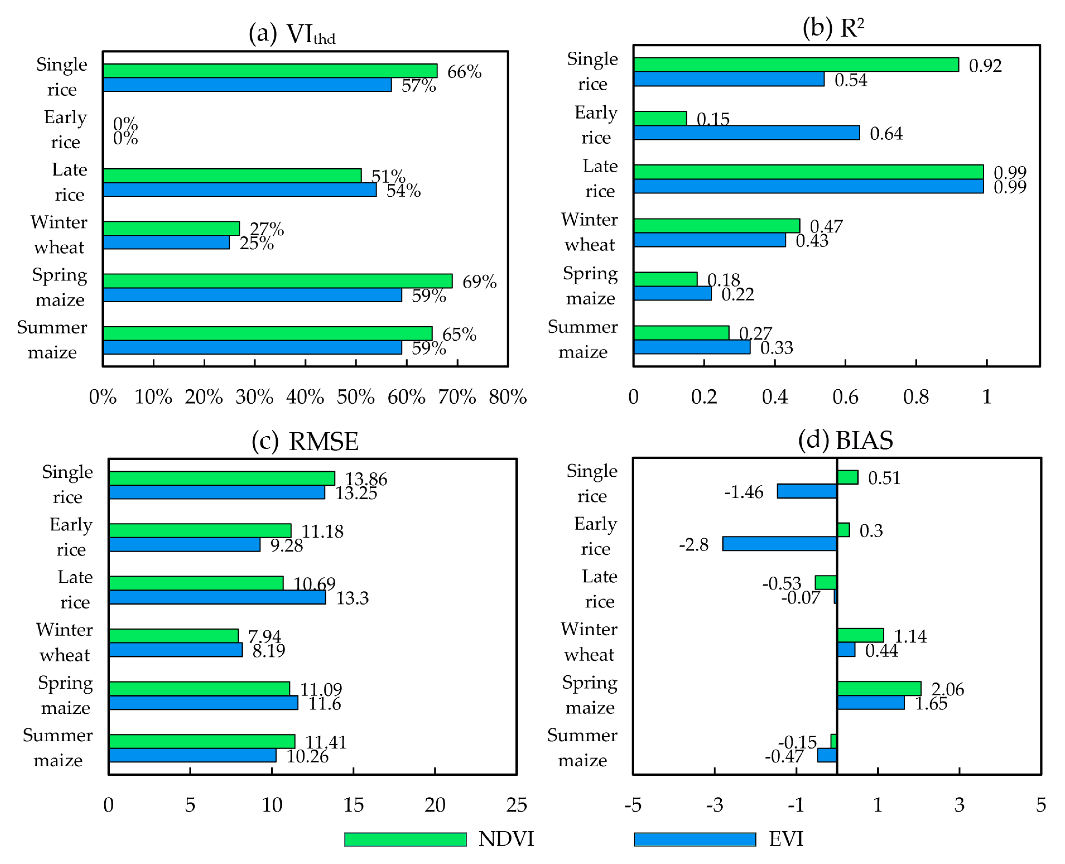
4.3. The Optimal Thresholds for Retrieving EOS

The optimization procedure for EOS was the same as that of SOS, but the pre-selected threshold range was from 0% to 35% for early rice and winter wheat, respectively, and the range was from 40% to 75% for the other crops. The results are shown in Figure 6. For most crops, as the threshold gradually increases, the R² increases first and then decreases. At the same time, the other statistics show the opposite trend. Only for early rice, the R² gradually decreases and never exceed 0.2. For single rice, spring maize, and summer maize, the optimal threshold is between 60% and 70%. For late rice, the optimal threshold is about 50%. For winter wheat and early rice, the optimal threshold is less than 30%, especially for early rice, which is approximately 0%.

The statistics of crop-specific optimal thresholds for retrieving EOS are shown in

Table 3. The optimal threshold for retrieving the end of the season (EOS) of each crop based on Normalized Difference Vegetation Index (NDVI).

Crop Types	$\mathbf{Number} \mathbf{of} \mathbf{Samples}$	$\mathit{V}{\mathit{I}}_{\mathit{t}\mathit{h}\mathit{d}}$	R2	RMSE (Days)	BIAS (Days)
Single rice	35	66%	0.92	13.9	0.5
Early rice	10	0%	0.15	11.2	0.3
Late rice	15	51%	0.99	10.7	−0.5
Winter wheat	36	27%	0.47	7.9	1.1
Spring maize	54	69%	0.18	11.1	2.1
Summer maize	34	65%	0.27	11.4	−0.2

. Among the six crops, the optimal threshold for spring maize, early rice, and summer maize are very high at 69%, 66%, and 65%, respectively. The optimal threshold for early rice and winter wheat were the lowest at 0% and 27%, respectively. In addition, the optimal threshold for late rice is 51%. The accuracy of the retrieved EOS of winter wheat is the highest, with R² of 0.47, RMSE of 7.9 days, and BIAS of 1.1 days. On the contrary, the accuracy of the retrieved EOS of single rice is lowest, with R² of 0.92, RMSE of 13.9 days, and BIAS of 0.5 days.

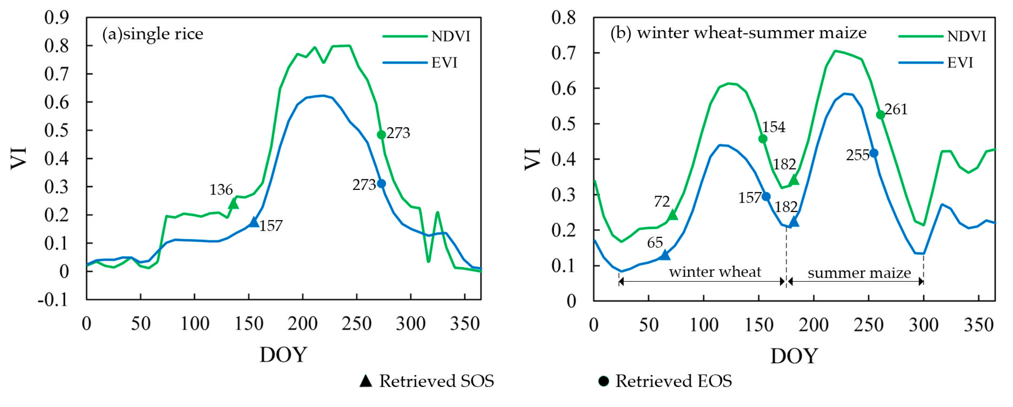
4.4. Comparison of the Retrieved SOS and EOS Based on NDVI and EVI

To compare the performance of NDVI and EVI in retrieving crop phenology, we obtain the SOS and EOS for each crop with the same procedure described above. The results of SOS and EOS are shown in Figure 7 and Figure 8, respectively. Except single rice, the optimal thresholds for retrieving SOS from NDVI are all slightly greater than that from EVI. In addition, for single rice and late rice, accuracies of the retrieved SOS from EVI are higher than their counterparts from NDVI. However, for spring maize and summer maize, accuracies of the SOS derived from NDVI are higher than the accuracies derived from EVI. For early rice and winter wheat, accuracies between SOS obtained from NDVI and EVI show no significant differences.

In terms of EOS, for most crops practiced in double cropping (early rice, late rice, winter wheat, and summer maize), the optimal thresholds based on NDVI are close to those based on EVI. However, for crops planted in single cropping (single rice and spring maize), the optimal thresholds for retrieving EOS based on NDVI are comparatively higher than those based on EVI by approximately 10%. For single rice, late rice, and winter wheat, accuracies of the retrieved EOS based on NDVI are higher than the retrieved EOS based on EVI. Especially for single rice, R² significantly increased when NDVI is used. For early rice and summer maize, however, accuracies of EOS obtained from EVI are higher than their counterpart from NDVI.

5. Discussion

5.1. Comparison of the Optimal Thresholds for Different Crops

As expected, the optimal SOS thresholds for crops planted in single cropping, and for the first crops of double cropping, are generally higher than those of other crops. Similarly, for EOS, the optimal thresholds for crops planted in single cropping, and the second crop of double cropping, are generally higher than those of other crops. This interesting phenomenon is rooted in the principle of the method itself. Indeed, the left or right minimum VI under those conditions are usually found during the winter months of January or December. During winter, usually extremely low vegetation cover is observed and the vegetation index is generally much lower compared to the rest of the year. Therefore, the threshold has to be relatively high to counterbalance the higher dynamic range in those situations (g₁ and g₂ in Figure 2b). For the other crops, however, the left minimum and the right minimum are the harvest period of the first crop. Crop maturity of the first crop and the emergence of the second crop are close to this point, which leads to smaller optimum threshold values. An example confirming this interpretation is shown in Figure 9 with the NDVI time-series of two ground stations: (a) single cropping with spring maize, and (b) double cropping of early rice-late rice.

5.2. Comparison of the Optimal Threshold Based on NDVI and EVI

According to Figure 7 and Figure 8, the optimal thresholds for retrieving SOS based on NDVI are generally slightly higher than those based on EVI. Moreover, for crops planted in single cropping (such as single rice and spring maize), the optimal threshold to retrieve EOS based on NDVI were significantly higher than those based on EVI. Taking single rice as an example, the optimal threshold for retrieving EOS based on NDVI is 66%, while the optimal threshold based on EVI is 57%. This finding mainly relates to the shape and amplitude of NDVI and EVI time series. Figure 10 shows an example of the NDVI and EVI time series of two stations for (a) single rice and (b) winter wheat-summer maize. As shown in Figure 10a, the amplitude and slope of NDVI time series are larger than the ones of the EVI time series in the growing season. Therefore, the optimal threshold for retrieving EOS needs to be larger. On the contrary, for SOS, the observation date is located at the position where the slope rises. Hence, there is little difference in the optimal threshold for retrieving SOS based on NDVI and EVI. In addition, as shown in Figure 10b, compared with the single-growing crops, the differences in shape and amplitude between NDVI and EVI time series of double-cropping are smaller. Therefore, the differences between the optimal thresholds for retrieving SOS and EOS from NDVI and EVI are also smaller.

5.3. Comparison of the Retrieval Accuracy Based on NDVI and EVI

The accuracies of the SOS results for single rice and late rice based on EVI are generally higher compared to NDVI. However, for spring maize and summer maize, we obtain opposite findings. In terms of EOS, for early rice and summer maize, results based on EVI have higher accuracy, but, for late rice and winter wheat, results based on NDVI are closer to the ground records. As an example, Figure 11 shows the NDVI and EVI time series from (a) a single rice station and (b) a spring maize station. As shown in Figure 11a, compared with NDVI, EVI has stronger anti-interference ability for the soil background, and is less influenced by noise. For low spatial resolution data (such as MODIS), most of the corresponding pixels in paddy rice fields are mixed pixels, which are often seriously affected by the surrounding land cover. Therefore, the phenology retrieval accuracy based on EVI is higher when compared to NDVI. However, as shown in Figure 11b, NDVI is more sensitive to chlorophyll than EVI, which leads to a larger growth amplitude that permits us to monitor vegetation growth more sensitively. When using remote sensing data of higher spatial resolution, the phenology retrieval accuracy of some crops based on NDVI may be higher [49,50].

5.4. Accuracy with Respect to Field Observations

Even using crop-specific optimal thresholds and vegetation indices, for single rice, late rice, spring maize, and summer maize, there are still comparatively large differences (RMSE greater than 10 days) between the satellite-based land surface phenology and the ground observations for SOS and EOS. Three main reasons are likely responsible for these findings.

(1)

The spatial resolution of MODIS data is rather coarse with respect to the field size, which leads to mixed pixel effects [51]. However, since the monitoring of vegetation phenology requires high temporal resolution, this limitation has to be accepted since few other sensors offer daily revisit capacity. However, as a consequence, the retrieval accuracy in small fields is low, especially in the south of China where the proportion of cultivated land is small, and the weather is usually cloudy and rainy.

(2)

Farmland ecosystems are strongly affected by human activities. Compared with natural vegetation, crop growth and development are affected by field management, breeding measures, use of different crop varieties, and varying planting patterns. Consequently, the resulting growth pattern and time series curves are more complex, and the retrieval accuracy is relatively lower when compared to forests and other natural vegetation types.

(3)

The scale differences between ground observations (point measurements) and the remote sensing data are huge and the two measurements do not record the same phenomenon. While the ground observation stations record the growth and development periods of individual fields (e.g., key phenological events), the remote sensing data mainly monitors the growth in biomass and leaf area index (LAI), i.e., the land surface phenology, at a much coarser scale [52].

6. Conclusions

Crop phenology is not only high on the academic agenda, but also of great practical importance. In order to investigate crop phenology accuracy based on the dynamic threshold method, we first improved the method to ensure a 100% retrieval rate. Only thereafter, the optimal crop-specific thresholds to retrieve the start of the season (SOS) and the end of the season (EOS) were determined based on ground observations, and the accuracy of the satellite-based estimates was assessed. In this respect, the performances based on Normalized Difference Vegetation Index (NDVI) and Enhanced Vegetation Index (EVI) were compared. From this study, the following conclusions are drawn.

(1)

The modified dynamic threshold method based on the proposed two growth amplitudes improves the retrieval success rate of SOS and EOS for crops, while maintaining or slightly improving the retrieval accuracy compared to the original method. It is, therefore, recommended to distinguish between pre-peak and post-peak periods when using the threshold method.

(2)

It is not appropriate to use identical thresholds to retrieve crop SOS and EOS. In particular, the commonly used 20% or 50% thresholds are not optimal for all crops. Moreover, large crop-specific differences for retrieving SOS and EOS for different crops and different cropping patterns have been observed. This leads to the recommendation that the crop type and the cropping pattern have to be determined prior to the land surface phenology (LSP) analysis, to permit application of crop-specific thresholds and to ensure optimum results.

(3)

As for SOS of single and late rice, the accuracies of the results based on EVI are slightly higher than those based on NDVI. However, for spring maize and summer maize, we obtain opposite findings. In terms of EOS, for early rice and summer maize, results based on EVI come with higher accuracy, but for late rice and winter wheat, results based on NDVI are closer to the ground records. These inconclusive results warrant more research, possibly including sites in other eco-regions. Whatever vegetation index is used, we recommend to carefully filter and smooth the data before analysis.

References

1. Rathcke, B.; Lacey, E.P. Phenological Patterns of Terrestrial Plants. Annu. Rev. Ecol. Syst. 1985, 16, 179–214. [Google Scholar] [CrossRef]
2. Atzberger, C. Advances in Remote Sensing of Agriculture: Context Description, Existing Operational Monitoring Systems and Major Information Needs. Remote. Sens. 2013, 5, 949–981. [Google Scholar] [CrossRef]
3. Wu, B.F.; Liu, C.L. Crop growth monitor system with coupling of NOAA and VGT data. In Proceedings of the Vegetation, Lake Maggiore, Italy, 3–6 April 2000; pp. 355–359. [Google Scholar]
4. Guérif, M.; Duke, C. Calibration of the SUCROS emergence and early growth module for sugar beet using optical remote sensing data assimilation. Eur. J. Agron. 1998, 9, 127–136. [Google Scholar] [CrossRef]
5. Boucher, O.; Myhre, G.; Myhre, A. Direct human influence of irrigation on atmospheric water vapour and climate. Clim. Dyn. 2004, 22, 597–603. [Google Scholar] [CrossRef]
6. Doraiswamy, P. Crop condition and yield simulations using Landsat and MODIS. Remote. Sens. Environ. 2004, 92, 548–559. [Google Scholar] [CrossRef]
7. Liu, F.; Chen, Y.; Shi, W.; Zhang, S.; Tao, F.; Ge, Q. Influences of agricultural phenology dynamic on land surface biophysical process and climate feedback. J. Geogr. Sci. 2017, 27, 1085–1099. [Google Scholar] [CrossRef]
8. Oteros, J.; García-Mozo, H.; Botey, R.; Mestre, A.; Galán, C. Variations in cereal crop phenology in Spain over the last twenty-six years (1986–2012). Clim. Change 2015, 130, 545–558. [Google Scholar] [CrossRef]
9. White, M.A.; De Beurs, K.M.; Didan, K.; Inouye, D.W.; Richardson, A.D.; Jensen, O.P.; O’Keefe, J.; Zhang, G.; Nemani, R.R.; Van Leeuwen, W.J.D.; et al. Intercomparison, interpretation, and assessment of spring phenology in North America estimated from remote sensing for 1982-2006. Glob. Chang. Boil. 2009, 15, 2335–2359. [Google Scholar] [CrossRef]
10. Parmesan, C.; Yohe, G. A globally coherent fingerprint of climate change impacts across natural systems. Nature 2003, 421, 37–42. [Google Scholar] [CrossRef]
11. Schwartz, M.D.; Ahas, R.; Aasa, A. Onset of spring starting earlier across the Northern Hemisphere. Global Change Biol. 2010, 12, 343–351. [Google Scholar] [CrossRef]
12. Richardson, A.D.; Braswell, B.H.; Hollinger, D.Y.; Jenkins, J.P.; Ollinger, S.V. Near-surface remote sensing of spatial and temporal variation in canopy phenology. Ecol. Appl. 2009, 19, 1417–1428. [Google Scholar] [CrossRef] [PubMed]
13. Hufkens, K.; Friedl, M.; Sonnentag, O.; Braswell, B.H.; Milliman, T.; Richardson, A.D. Linking near-surface and satellite remote sensing measurements of deciduous broadleaf forest phenology. Remote Sens. Environ. 2012, 117, 307–321. [Google Scholar] [CrossRef]
14. Richardson, A.; Jenkins, J.; Braswell, B.D.; Ollinger, S.; Smith, M. Use of digital webcam images to track spring green-up in a deciduous broadleaf forest. Oecologia 2007, 152, 323–334. [Google Scholar] [CrossRef] [PubMed]
15. Sonnentag, O.; Hufkens, K.; Tesherasterne, C.; Young, A.M.; Friedl, M. Digital repeat photography for phenological research in forest ecosystems. Agric. For. Meteorol. 2012, 152, 159–177. [Google Scholar] [CrossRef]
16. Atkinson, P.M.; Jeganathan, C.; Dash, J.; Atzberger, C. Inter-comparison of four models for smoothing satellite sensor time-series data to estimate vegetation phenology. Remote Sens. Environ. 2012, 123, 400–417. [Google Scholar] [CrossRef]
17. White, M.A.; Nemani, R.R. Real-time monitoring and short-term forecasting of land surface phenology. Remote Sens. Environ. 2006, 104, 43–49. [Google Scholar] [CrossRef]
18. Ren, S.; Qin, Q.; Ren, H. Contrasting wheat phenological responses to climate change in global scale. Sci. Total Environ. 2019, 665, 620–631. [Google Scholar] [CrossRef]
19. Vrieling, A.; Meroni, M.; Darvishzadeh, R.; Skidmore, A.K.; Wang, T.; Zurita-Milla, R.; Oosterbeek, K.; O’Connor, B.; Paganini, M. Vegetation phenology from Sentinel-2 and field cameras for a Dutch barrier island. Remote Sens. Environ. 2018, 215, 517–529. [Google Scholar] [CrossRef]
20. Delécolle, R.; Maas, S.J.; Guerif, M.; Baret, F. Remote sensing and crop production models: present trends. ISPRS J. Photogramm. Remote Sens. 1992, 47, 145–161. [Google Scholar] [CrossRef]
21. Zhang, X. Land Surface Phenology: Climate Data Record and Real-Time Monitoring. In Comprehensive Remote Sensing; Liang, S., Ed.; Elsevier: Oxford, UK, 2018; pp. 35–52. [Google Scholar]
22. Ganguly, S.; Friedl Mark, A.; Tan, B.; Zhang, X.; Verma, M. Land surface phenology from MODIS: Characterization of the Collection 5 global land cover dynamics product. Remote Sens. Environ. 2010, 114, 1805–1816. [Google Scholar] [CrossRef]
23. Curnel, Y.; Oger, R. Agrophenology indicators from remote sensing: state of the art. In Proceedings of the ISPRS Archives XXXVI-8/W48 Workshop proceedings: Remote sensing support to crop yield forecast and area estimates, Stresa, Italy, 30 November–1 December 2006; pp. 31–38. [Google Scholar]
24. Fischer, A. A model for the seasonal variations of vegetation indices in coarse resolution data and its inversion to extract crop parameters. Remote. Sens. Environ. 1994, 48, 220–230. [Google Scholar] [CrossRef]
25. Lloyd, D. A phenological classification of terrestrial vegetation cover using shortwave vegetation index imagery. Int. J. Remote. Sens. 1990, 11, 2269–2279. [Google Scholar] [CrossRef]
26. Jonsson, P.; Eklundh, L. Seasonality extraction by function fitting to time-series of satellite sensor data. IEEE Trans. Geosci. Remote. Sens. 2002, 40, 1824–1832. [Google Scholar] [CrossRef]
27. White, M.A.; Thornton, P.E.; Running, S.W. A continental phenology model for monitoring vegetation responses to interannual climatic variability. Global Biogeochem. Cycles 1997, 11, 217–234. [Google Scholar] [CrossRef]
28. Duchemin, B.T.; Goubier, J.M.; Courrier, G. Monitoring phenological key stages and cycle duration of temperate deciduous forest ecosystems with NOAA/AVHRR data. Remote Sens. Environ. 1999, 67, 68–82. [Google Scholar] [CrossRef]
29. Reed, B.C.; Brown, J.F.; Vanderzee, D.; Loveland, T.R.; Merchant, J.W.; Ohlen, D.O. Measuring phenological variability from satellite imagery. J. VEG. SCI. 1994, 5, 703–714. [Google Scholar] [CrossRef]
30. Beck, P.S.A.; Atzberger, C.; Hogda, K.A.; Johansen, B.; Skidmore, A.K. Improved monitoring of vegetation dynamics at very high latitudes: A new method using MODIS NDVI. Remote Sens. Environ. 2006, 100, 321–334. [Google Scholar] [CrossRef]
31. Zhang, X.; Friedl, M.A.; Schaaf, C.B.; Strahler, A.H.; Hodges, J.C.F.; Gao, F.; Reed, B.C.; Huete, A. Monitoring vegetation phenology using MODIS. Remote Sens. Environ. 2003, 84, 471–475. [Google Scholar] [CrossRef]
32. Sakamoto, T.; Yokozawa, M.; Toritani, H.; Shibayama, M.; Ishitsuka, N.; Ohno, H. A crop phenology detection method using time-series MODIS data. Remote Sens. Environ. 2005, 96, 366–374. [Google Scholar] [CrossRef]
33. Atzberger, C.; Eilers, P.H.C. A time series for monitoring vegetation activity and phenology at 10-daily time steps covering large parts of South America. Int. J. Digital Earth 2011, 4, 365–386. [Google Scholar] [CrossRef]
34. Cong, N.; Piao, S.; Chen, A.; Wang, X.; Lin, X.; Chen, S.; Han, S.; Zhou, G.; Zhang, X. Spring vegetation green-up date in China inferred from SPOT NDVI data: A multiple model analysis. Agric. For. Meteorol. 2012, 165, 104–113. [Google Scholar] [CrossRef]
35. Delbart, N.; Beaubien, E.; Kergoat, L.; Toan, T.L. Comparing land surface phenology with leafing and flowering observations from the PlantWatch citizen network. Remote Sens. Environ. 2015, 160, 273–280. [Google Scholar] [CrossRef]
36. Yu, H.Y.; Luedeling, E.; Xu, J.C. Winter and spring warming result in delayed spring phenology on the Tibetan Plateau. Proc. Natl. Acad. Sci. USA 2010, 107, 22151–22156. [Google Scholar] [CrossRef] [PubMed] [Green Version]
37. Wu, C.Y.; Peng, D.L.; Soudani, K.; Siebicke, L.; Gough, C.M.; Arain, M.A.; Bohrer, G.; Lafleur, P.M.; Peichl, M.; Gonsamo, A.; et al. Land surface phenology derived from normalized difference vegetation index (NDVI) at global FLUXNET sites. Agric. For. Meteorol. 2017, 171–182. [Google Scholar] [CrossRef]
38. Guo, L.; An, N.; Wang, K. Reconciling the discrepancy in ground- and satellite-observed trends in the spring phenology of winter wheat in China from 1993 to 2008. J. Geophys. Res.: Atmos. 2016, 121, 1027–1042. [Google Scholar] [CrossRef] [Green Version]
39. Alcantara, C.; Kuemmerle, T.; Prishchepov, A.V.; Radeloff, V.C. Mapping abandoned agriculture with multi-temporal MODIS satellite data. Remote Sens. Environ. 2012, 124, 334–347. [Google Scholar] [CrossRef]
40. Wu, W.B.; Peng, Y.; Tang, H.J.; Zhou, Q.B.; Chen, Z.X.; Shibasaki, R. Characterizing spatial patterns of phenology in cropland of China based on remotely sensed data. Agric. Sci. Chin. 2010, 9, 101–112. [Google Scholar] [CrossRef]
41. Ogle, S.M.; Breidt, F.J.; Paustian, K. Agricultural management impacts on soil organic carbon storage under moist and dry climatic conditions of temperate and tropical regions. Biogeochemistry 2005, 72, 87–121. [Google Scholar] [CrossRef]
42. Biradar, C.M.; Xiao, X. Quantifying the area and spatial distribution of double- and triple-cropping croplands in India with multi-temporal MODIS imagery in 2005. Int. J. Remote Sens. 2011, 32, 367–386. [Google Scholar] [CrossRef]
43. Liu, J.; Zhu, W.; Atzberger, C.; Zhao, A.; Pan, Y.; Huang, X. A phenology-based method to map cropping patterns under a wheat-maize rotation using remotely sensed time-series data. Remote Sens. 2018, 10. [Google Scholar] [CrossRef] [Green Version]
44. Atzberger, C.; Formaggio, A.R.; Shimabukuro, Y.E.; Udelhoven, T.; Mattiuzzi, M.; Sanchez, G.A.; Arai, E. Obtaining crop-specific time profiles of NDVI: the use of unmixing approaches for serving the continuity between SPOT-VGT and PROBA-V time series. Int. J. Remote Sens. 2014, 35, 2615–2638. [Google Scholar] [CrossRef]
45. Liu, J.; Zhan, P. The impacts of smoothing methods for time-series remote sensing data on crop phenology extraction. In Proceedings of the 2016 IEEE International Geoscience and Remote Sensing Symposium (IGARSS), Beijing, China, 10–15 July 2016; pp. 2296–2299. [Google Scholar]
46. Zhu, W.; Pan, Y.; He, H.; Wang, L.; Mou, M.; Liu, J. A changing-weight filter method for reconstructing a high-quality NDVI time series to preserve the integrity of vegetation phenology. IEEE Trans. Geosci. Remote Sens. 2012, 50, 1085–1094. [Google Scholar] [CrossRef]
47. Jönsson, P.; Eklundh, L. TIMESAT—a program for analyzing time-series of satellite sensor data. Comput. Geosci. 2004, 30, 833–845. [Google Scholar] [CrossRef] [Green Version]
48. Richter, K.; Atzberger, C.; Hank, T.B.; Mauser, W. Derivation of biophysical variables from earth observation data: validation and statistical measures. J. Appl. Remote Sens. 2012, 6, 063557. [Google Scholar] [CrossRef]
49. Peng, D.; Wu, C.; Li, C.; Zhang, X.; Liu, Z.; Ye, H.; Luo, S.; Liu, X.; Hu, Y.; Fang, B. Spring green-up phenology products derived from MODIS NDVI and EVI: Intercomparison, interpretation and validation using National Phenology Network and AmeriFlux observations. Ecol. Indic. 2017, 323–336. [Google Scholar] [CrossRef]
50. Zhang, X.; Jayavelu, S.; Liu, L.; Friedl, M.A.; Henebry, G.M.; Liu, Y.; Schaaf, C.B.; Richardson, A.D.; Gray, J. Evaluation of land surface phenology from VIIRS data using time series of PhenoCam imagery. Agric. For. Meteorol. 2018, 137–149. [Google Scholar] [CrossRef]
51. Liu, L.; Cao, R.; Shen, M.; Chen, J.; Wang, J.; Zhang, X. How does scale effect influence spring vegetation phenology estimated from satellite-derived vegetation indexes? Remote Sens. 2019, 18, 2137. [Google Scholar] [CrossRef] [Green Version]
52. Hanes, J.M.; Liang, L.; Morisette, J.T. Land surface phenology. In Biophysical Applications of Satellite Remote Sensing; Hanes, J.M., Ed.; Springer: Berlin/Heidelberg, Germany, 2014; pp. 99–125. [Google Scholar]
Figure 1. Location of the ground observation stations.
Remotesensing 11 02725 g001
Figure 2. Illustration of the dynamic threshold method before (a) and after modification (b), x-axis represents Day of Year (DOY), and y-axis represents the Vegetation Index (VI). Instead of using a single VI dynamic range, the modified algorithm distinguishes between ascending and descending growth curves.
Remotesensing 11 02725 g002
Figure 3. Comparison of the start of the season (SOS) retrieval results before (gray bars) and after algorithm improvement (orange bars), and both are based on the 20% amplitude threshold. (a) B, (b) Coefficient of determination (R2), (c) Root Mean Square Error (RMSE), (d) BIAS.
Remotesensing 11 02725 g003
Figure 4. Comparison of the end of the season (EOS) retrieval results before (gray bars) and after algorithm improvement (orange bars), and both are based on the 20% amplitude threshold (a) B, (b) Coefficient of determination (R2), (c) Root Mean Square Error (RMSE), (d) BIAS.
Remotesensing 11 02725 g004
Figure 5. Crop-specific the start of the season (SOS) retrieval accuracies based on Normalized Difference Vegetation Index (NDVI) under different thresholds.
Remotesensing 11 02725 g005
Figure 6. Crop-specific the end of the season (EOS) retrieval accuracies based on Normalized Difference Vegetation Index (NDVI) under different thresholds.
Remotesensing 11 02725 g006
Figure 7. Optimal thresholds and corresponding accuracies of the retrieved the start of the season (SOS) based on Normalized Difference Vegetation Index (NDVI) (green) and Enhanced Vegetation Index (EVI) (blue). (a) The optimal threshold (VIthd), (b) Coefficient of determination (R2), (c) Root Mean Square Error (RMSE), (d) BIAS.
Remotesensing 11 02725 g007
Figure 8. The optimal thresholds and the corresponding accuracies of the retrieved the end of the season (EOS) based on Normalized Difference Vegetation Index (NDVI) (green) and Enhanced Vegetation Index (EVI) (blue). (a) The optimal threshold (VIthd), (b) Coefficient of determination (R2), (c) Root Mean Square Error (RMSE), (d) BIAS.
Remotesensing 11 02725 g008
Figure 9. Representative Normalized Difference Vegetation Index (NDVI) time series curves of (a) spring maize and (b) early rice-late rice.
Remotesensing 11 02725 g009
Figure 10. Differences of the retrieved the start of the season (SOS) and the end of the season (EOS) based on Normalized Difference Vegetation Index (NDVI) (in green) and Enhanced Vegetation Index (EVI) time series (in blue) with (a) single rice and (b) winter wheat-summer maize.
Remotesensing 11 02725 g010
Figure 11. Examples of Normalized Difference Vegetation Index (NDVI) (in green) and Enhanced Vegetation Index (EVI) time series (in blue) of (a) single rice and (b) spring maize.
Remotesensing 11 02725 g011