Automated Inspection of Railway Tunnels’ Power Line Using LiDAR Point Clouds


1
Department of Materials Engineering, Applied Mechanics and Construction, School of Industrial Engineering, University of Vigo, 36310 Vigo, Spain
2
Department of Natural Resources and Environmental Engineering, School of Mining Engineering, University of Vigo, 36310 Vigo, Spain
*
Author to whom correspondence should be addressed.
Remote Sens. 2019, 11(21), 2567; https://doi.org/10.3390/rs11212567
Submission received: 10 September 2019
/
Revised: 29 October 2019
/
Accepted: 30 October 2019
/
Published: 1 November 2019
(This article belongs to the Special Issue Inland Transport Networks Monitoring from Remote Sensing and Photogrammetry)
Abstract
:Transport networks need periodic inspections to increase their safety and improve their management. In the last few years, LiDAR (light detection and ranging) technology has become a tool for helping to create a precise database of almost any type of infrastructure. Mobile laser scanning (MLS) systems use a laser beam to collect dense three dimensional (3D) point clouds, which include geometric and radiometric data of the environment in which they are placed. In the context of this paper, a methodology for automatically inspecting the clearance gauge and the deflection of the aerial contact line in railway tunnels is presented. The main objective is to compare results and verify their compliance with the Spanish norm. The 3D data are provided by a LYNX Mobile Mapper System (MMS). First, the area is surveyed and then the obtained (3D) point cloud is classified into contact wire, suspension wire, and remaining points. Finally, the inspection of the railway’s power line is performed. The validation of the proposed methodology has been carried out in three different tunnel point clouds, obtaining both qualitative and quantitative results for points’ classification, together with the results of the measures performed.
1. Introduction
Nowadays, the interest of having a digital model of real-life scenarios is increasing. This model can be used to update and track the behaviour of an infrastructure through its whole life cycle. In the railway field, with the arrival of the high-speed train and the high request for its maintenance and inspection, research concerning technical and technological improvements has increased. One of the main concerns of the railway industry is the irregularities affecting the rail track layout, as well as the perfect state of the catenary to fulfil the requirements of gauge, among others. These elements have a big repercussion in the security of the whole railway system. Hence, railway companies invest their resources for the optimal inspection and maintenance of the infrastructures. This is where laser scanning systems come into consideration. In recent years, the applications for laser scanning technology have increased. Until now, the main applications involving this type of data were dimensional control [1], 3D modelling, urban planning, and, more recently, BIM (building information modelling). The main characteristic of laser scanners is their capacity for obtaining large amounts of data with high accuracy in a short period of time. Usually, this information was processed manually or semi-automatically. The monotony of this task called for the necessity of automatically process the generated three dimensional (3D) point clouds.
This work arises due to the lack of specific methods for classifying and inspecting railway point clouds, and especially railway power lines. It is focused on the automatic classification of MLS point clouds of the aerial contact line system from railway tunnels, and its later inspection. The aerial contact line is a set of overhead cables on top of the railway line. They provide electrical supply to electric trains. These cables are placed over the vehicle’s superior gauge limit, being the electrical supply provided through pantographs [2]. The system is composed by three different categories of cables: (i) Contact wire, from which the pantograph takes the power for the train; (ii) suspension or catenary wire, which resists and supports the catenary weight and keeps the contact wire in a constant height; and (iii) droppers, which are vertical elements that help to maintain the contact wire in that constant height, and are fixed in between the suspension and the contact wire. These three types of elements are hanged over the train’s car with poles or cantilever arms [3].
The present paper is divided into the next sections: Section 2 presents a review of the literature related with this work; Section 3 explains the methodology, which is in charge of the classification of points conforming both the contact and the suspension wires, and the inspection of these cables; Section 4 describes the equipment used for the data gathering; Section 5 exposes the results obtained for the datasets on disposal; and, lastly, the conclusions to this research together with future lines of work to be considered are exposed in Section 6.
2. Literature Review
Although some authors have developed methods using data from both aerial laser scanning (ALS) and terrestrial laser scanning (TLS) systems in the railway environment [4,5,6], the most common approach is to work with mobile laser scanning (MLS) point clouds. The use of MLS systems is translated into safer and faster surveys, obtaining data with very high accuracy and quality [7]. In this relation, Che et al. [8] presented also a review about the most recent object recognition, segmentation, and classification methods for LiDAR (light detection and ranging) data. With regard to the railway field, some authors have also developed different techniques for LiDAR-data grouping. Leslar et al. [9] propose a first classification of points regarding their return number, and then they perform a manual classification by using specific programs and semi-automatic methods. Several works from Arastounia propose heuristic methods for the fully-automatic classification of railway objects [10,11,12]. These objects such as rails, contact lines or catenaries, are extracted through an algorithm that recognizes interesting objects when studying how the LiDAR data are placed and their spatial relation with each other and with other objects. The result is a classified point cloud that can be used for later analysis, namely 3D modelling, specific measurements, or inspection of the continuity of rails. Concerning power line classification from 3D point clouds, Arastounia improved his own methods creating an algorithm for the recognition of railroad power lines and rail tracks using both Terrestrial Laser Scanning (TLS) and Aerial Laser Scanning (ALS) data [11]. Apart from these works, when focusing on the power line detection, Pastucha [13] used the trajectory data to limit the searching zone for extracting the power line. Then, RANSAC (RANdom SAmple Consensus) algorithms and geometrical relationships were used to improve the points’ classification. In this relation, Zhang et al. [14] also used information from the MLS trajectory to extract valuable data from it, subsequently applying region growing algorithms to classify aerial contact wires’ points. Similar to the railway field, point clouds from high voltage facilities or roadways have also been explored in order to classify their points. To this respect, Guo et al. [15] proposed a method for the reconstruction of wires working with ALS data, and applying RANSAC algorithms. Later on, Wang et al. [16] presented a methodology for detecting power line points and the power line corridor direction using connectivity and simplification algorithms. With reference to the inspection of railway power lines, authors like Blug et al. started to use laser scanning data for clearance measurements [17]. Years later and with recent equipment, Mikrut et al. [18] used cross-sectional data from point clouds to create 2D images that could be visually inspected by an expert in order to find anomalies.
Currently, the trend is to use classifiers in order to make predictions of points’ classes. In this sense, Luo et al. [19] used the Conditional Random Field (CRF) classifier in order to make a context-based classification of the LiDAR points into several classes (railway elements). Using not only heuristic methods but also support vector machines (SVMs), Sánchez-Rodríguez et al. [20] presented a methodology for the classification of elements in an MLS railway tunnel point cloud. The good performance of deep learning algorithms for image classification has encouraged authors to develop new models for 3D data [21,22,23,24]. In this field, not only MLS but also ALS data are used to test the new convolutional networks used for point cloud classification. Balado et al. [25] use ALS for the automatic classification of land cover using the classifier ResNet-50, and in a later work, proved the validity of PointNet for MLS point clouds’ classification [26]. Although many authors are working to improve these methods [27,28], they still need to evolve.
The novelty of this paper is the presentation of a fully automated method for measuring the power line gauge and the catenary deflection in a LiDAR point cloud, without the need of human intervention. The method is in charge of classifying points forming both the contact and the suspension wire, and then performing the corresponding measures.
3. Methodology
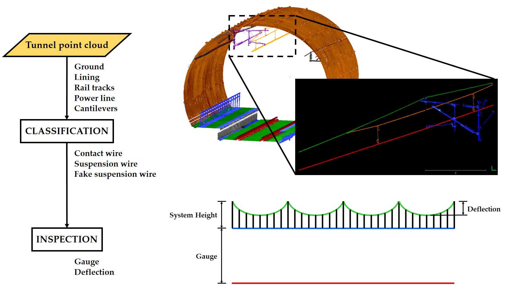
This paper follows the steps previously set in [20], where a methodology for the automatic classification of railway tunnel elements from MLS datasets was presented. The present work is oriented to the development and analysis of a new system for the recognition, classification, and inspection of electrical railway infrastructures using LiDAR data. The work starts with a labelled point cloud divided into lining, ground, railway tracks, overhead line, and cantilevers. This information is extracted following the steps presented in [20], and as reflected in Figure 1. In this section, the method developed for the automatic inspection of railway tunnels’ power line is presented. First, Section 3.1 describes the steps followed to classify the contact wire and suspension wire points. Then, Section 3.2 exposes the inspection methods developed for measuring both the clearance gauge and the deflection of the suspension wire.
It is important to highlight that there are different catenary models installed in Spain, in the Conventional Network of Adif (Red Convencional de Adif). The most outstanding ones due to their common implementation are models CA-160 and CA-220, which are taken as reference for the present work [2,3]. The parameters used in this work for the segmentation of the catenary system and its inspection follow the standards summarized in Table 1.
3.1. Classification of Points
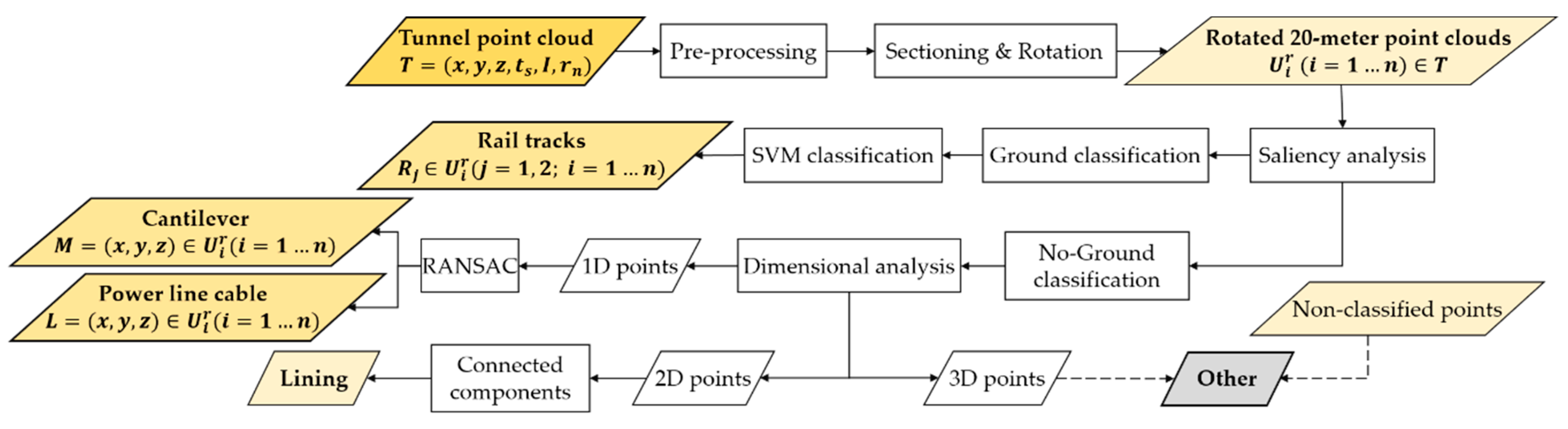
The method developed for this work is based on the one advanced by Sánchez-Rodríguez et al. [20]. Following the previously developed methodology, the method starts with a railway tunnel point cloud , where are the three-dimensional (3D) spatial coordinates, is the time stamp, is the reflected laser pulse intensity, and is the return number assigned to each point. Since these point clouds have too much information to be processed by regular computers, the tunnel point cloud is segmented into 20-m long sections, , and each of them is oriented to the y coordinate axis, resulting . Subsequently, continuing with the algorithms proposed in [20], every element in the tunnel point cloud ends up classified based on its geometrical characteristics as ground, lining, power line, cantilever arms, rails, and other (Figure 1). For the research of this paper, some of these classified points are used as basis before starting to develop the new classification methods. These are the ones forming rails and power lines, together with cantilever arms. It is important to highlight that, in the previous classification, the power lines were saved as individual sets of points, since there might be more than one in each 20-m section.
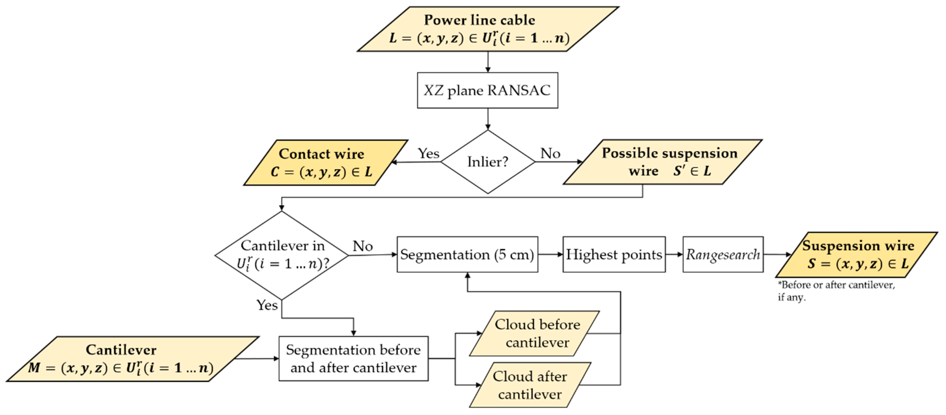
The novel classification algorithms presented in this work are summarized in Figure 2, and fully described in Section 3.1.1 and Section 3.1.2.
3.1.1. Contact wire detection
Let be the point cloud of an individual power line. The first step is to distinguish the contact wire from the suspension wire and other elements (droppers and fake suspension wire, which allow the elasticity’s homogeneity through the line [29]). Using point cloud as the basis, the RANSAC method is applied to find the contact cable. To do that, the point cloud is rasterized so that it is mapped to the YZ plane [30]. Then, the predefined Matlab function fitPolynomialRANSAC is applied [31]. It uses a version of the original RANSAC called M-estimator SAmple Consensus (MSAC), which finds the coefficients of a polynomial of degree that best fits the input data. In the described case, the need is to fit a line to the two-dimensional (2D) cloud, so the coefficient must be . The aforementioned function is iterative, meaning that the fitting process is repeated until it reaches the convergence. This happens when achieving the maximum number of possible iterations or the predefined precision (number of points fitting the line, in this case). In order to obtain a better tuning, the function uses the maximum allowed distance along the Z axis from an inlier to the estimated polynomial. This parameter was set to 0.15 m as the section of the CA-220 contact wire is 150 mm2 (the diameter would be 13.8 mm), as reflected in Table 1. Inliers coming, as a result, are the points forming the contact wire (Figure 2).
3.1.2. Suspension wire detection
For detecting the suspension wire, a different approach has been followed. Since this cable is always located in the maximum height of the remaining non-classified points of the power line, a search on this basis is started. In this part of the segmentation process, it is necessary to know where the cantilevers are placed, as the highest points of the catenary curve drawn by these cables depend on them. Taking into account that the sections performed in the original point cloud are 20 m long, and following the established in the ADIF specifications [3] concerning the ‘distance between cantilevers’ in railway tunnels (50 m), only one cantilever can be contained in each of these sections.
Let be the possible suspension wire cloud. For the case that the selected section contains a cantilever, the point cloud will be sectioned in two parts: one before and one after this element. Then, in order to improve the effectiveness of the algorithm, points belonging to these two parts are studied, segmenting the cloud into 5 cm sections (Figure 3). After that, a search of valid points is performed starting with the highest points of these small sections. In this case, the broadly known range search algorithm is chosen for this matter [31]. The algorithm finds all neighbours in that are within a distance from each of the highest ones selected before. In this case, that distance is taken as the standardized diameter of the suspension wire (Table 1). If, in the selected section , no cantilevers are present, the algorithm is executed without distinguishing two parts in the cloud (Figure 2).
3.2. Gauge and Deflection
In a railway line, gauge (officially called contact wire height) is the distance between the inferior plane of the contact wire and the running surface (tangent to the rails’ heads). This distance is perpendicularly measured in the axis of the track (Euclidean distance). Together with this, the deflection is defined as the maximum vertical distance existing between the suspension wire and the imaginary line joining two consecutive cantilevers. These distances are graphically represented in Figure 4.
The algorithm in charge of measuring the clearance gauge starts with the contact wire () and the rails’ point clouds (). First, a plane is fitted to the top surface of rails. To do that, the voxelization of the rails’ point cloud is done. Then, voxels with the biggest z coordinate are used as the rails’ top surface, and after that, a search to find the plane that best fits them is started. To continue with the process, the point cloud forming the contact cable is also voxelized so that only one point is saved inside each 50 cm imaginary cube (voxel). Finally, the Euclidean distance between these new points (one per voxel) and the previously fitted plane is measured, following Equation (1):
where q and p are the two points from which the distance is measured. The result are several measures in each 20-m section (Figure 5a).
For the measurement of the suspension wire deflection, it is first necessary to find which sections contain a cantilever . Then, the suspension wire point clouds placed between two consecutive cantilevers are grouped, as shown in Figure 6. The next step is to draw a line joining the two most extreme points of the span. These two points are located in the highest z coordinate in each of the two points clouds containing a cantilever (Figure 6). Finally, the deflection is measured. This is done by calculating the maximum distance between the previously fitted line and each point in the point cloud sections forming a span (Figure 5b). As a result, only one measure is obtained for each span in the tunnel point cloud .
4. Equipment Setup
Laser scanning systems use a laser beam to generate a 3D model of the objects in the environment of study. The objects are represented with 3D coordinates in the space, obtained computing the distance between the LiDAR sensor and the target object. As laser scanners are an active technology, surveys can be performed at night or in places like tunnels, where the light has very low intensity. In this work, data have been obtained using a LYNX Mobile Mapper, by Optech Inc. (2007) [32]. The summary of its characteristics and a specific accuracy analysis is shown in [33]. The LiDAR sensor together with the position and navigation systems, and the four racks (acquisition, control, LiDAR, and power supply), were placed in a draisine to ease the data acquisition process inside railway tunnels.
4.1. Geo-Referencing and Sensor Fusion
The positioning and navigation systems in charge of the 3D data positioning are also a key issue when performing a laser scanning survey. This is supported by GNSS (Global Navigation Satellite System) and INS (inertial navigation system) systems that require a specific planning for every measurement campaign. GNSS provides position and orientation with respect to a reference, while INS and DMI (distance measurement unit) provide time-derivative information of the position and orientation of the mobile platform. Using this information, the position of the point cloud at global level is determined: (i) the point cloud is referenced with respect to the LiDAR sensor itself; (ii) the platform is located with reference to the WGS84 global coordinate system; and (iii), the relative orientation and position of the LiDAR sensor in the platform with regard to the navigation and position system is determined.
4.2. Performance
Since every survey requires different planning before the performance, it is necessary to consider the particular needs of each case study. In general, the data acquisition time depends on the vehicle’s average speed, which varies between 20 and 30 km/h. Apart from this, the total work time also includes: (a) equipment installation, which takes between half a day and a whole day depending on the draisine structure; (b) moving to the capture zone, with a speed similar to the data acquisition one; (c) data gathering (20–30 km/h); and (d) uninstalling the equipment, which usually takes around half a day. In addition, the performance of the Lynx Mobile Mapper is given by its resolution. Information about the equipment’s acquisition parameters can be found in Table 2.
Changes in the accuracy of point clouds are noticeable regarding the equipment with which they were acquired. There are three types of errors leading to low accuracy (in general) in laser scanners [34]:
- Laser range error: measuring the distance to an object. It is different for every scanner and can be corrected by recalibrating them (by the manufacturer or specialist in the field).
- Range noise: deviation of single readings from the real value within a sample of measures. It is conditioned by the distance to the object to be scanned and the reflectivity of the object’s material.
- Mechanical error: the difference between the measured and actual horizontal and vertical angles (angular error). It is caused by the mechanical devices forming the laser scanner (mirrors and servos).
The position and navigation systems may also result in invalid coordinates for the GNSS base station(s), misalignment of the INS with the LiDAR scanner, or a software failure at coordinate conversions. These cause systematic errors that may be identified by sensor calibration, comparing LiDAR with known reference data or additional control operations [35].
It is important to highlight that accuracy depends not only on the equipment, but also on the geometry of the 3D scenario under study. This affects to the performance of the trajectory and point cloud computation algorithms, and so a specific value of accuracy cannot be given as an answer. The atmospheric condition can also have undesired effects in the LiDAR performance that could lead to noisy measurements [36].
5. Results
The classification of the aerial contact line points is developed using the algorithms described in Section 3.1. The data is classified into four categories: contact wire, suspension wire and remaining points. Then, the gauge of the contact wire and the deflection of the suspension wire are inspected following the current Spanish standards, as explained in Section 3.2.
In this section, the classification and inspection results are detailed. The methodology is implemented using the Matlab software, version 2017b. The validation performance is done using an Intel Core i7-4810MQ CPU at 2.8 GHz and 8 GB of RAM.
5.1. Case Study
The classification part of this work has been proved as valid in three different tunnel point clouds extracted from Spanish corridors, which are divided into 20-m sections so that the classification process can be performed by a regular computer (Table 3). Although one of the tunnels (tunnel C) has two power lines on top of the rails, the developed methodology would only consider the detection of the one in the closest area to the laser scanning system. Moreover, this tunnel dataset has only one cantilever present, hence the deflection measurement of the suspension wire cannot be tested on it.
5.2. Classification Results
This section exposes the classification results obtained for each of the three tunnel point clouds. In order to prove the validity of the method, one 20-m section of each dataset is selected. The characteristics of these points clouds are presented in Table 4.
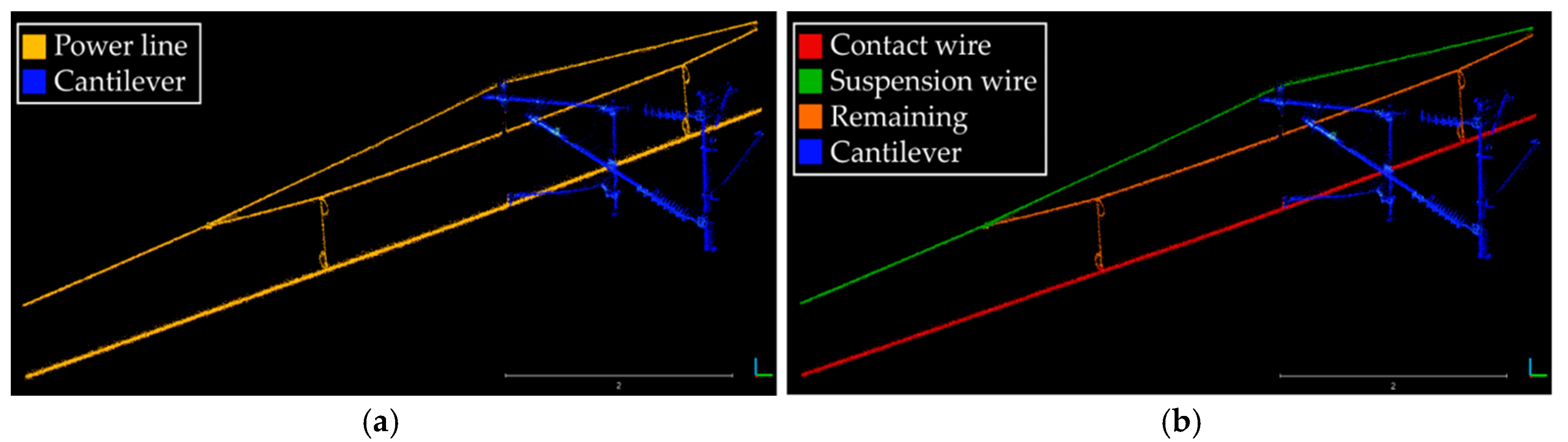
The contact wire points are first classified and separated from the rest of the point cloud, so it is prepared for the next segmentation step. Then, points belonging to the suspension wire are identified, these data being enough to perform the inspection required. After this classification of the aerial contact line elements, each point in the original cloud ended up labelled as contact wire, suspension wire or remaining points. The cantilever classification results are extracted from the previously developed methodology [20], and an overview of the whole power line classification is presented in Figure 7. This figure shows the original point cloud used for the classification process of this work (Figure 7a), making a distinction between the power line cables in general and the cantilevers present in the cloud (if any). Then, in Figure 7b points are depicted with different colours as belonging to specific groups: contact wire, suspension wire, and remaining (droppers and other cables), showing again the cantilever present and previously classified in the cloud.
As a way of proving the validity of the methods proposed, datasets from Table 4 are used. This prove is performed by quantitative comparing a previously labelled ground truth with the obtained results. The ground truth is labelled manually thanks to the use of the 3D point cloud processing software CloudCompare (v2.10.2). The precision, recall, and F-score performance metrics have been calculated for each of the three selected sections, and the results are exposed in Table 5.
where TP is the number of true positives; FP is the number of false positives; and FN is the number of false negatives.
These results show high performance metrics for the classification tasks developed under the scope of this work.
5.3. Inspection Results
The classification results of the three tunnel point clouds are used for the validation of the automatic inspection method. In order to ease the process of the results’ discussion, the distances obtained for the gauge measurement are exposed graphically and for the 20-m point cloud of Tunnel A exposed in Table 6. However, the point clouds used to present the deflection results are the ones in Table 6.
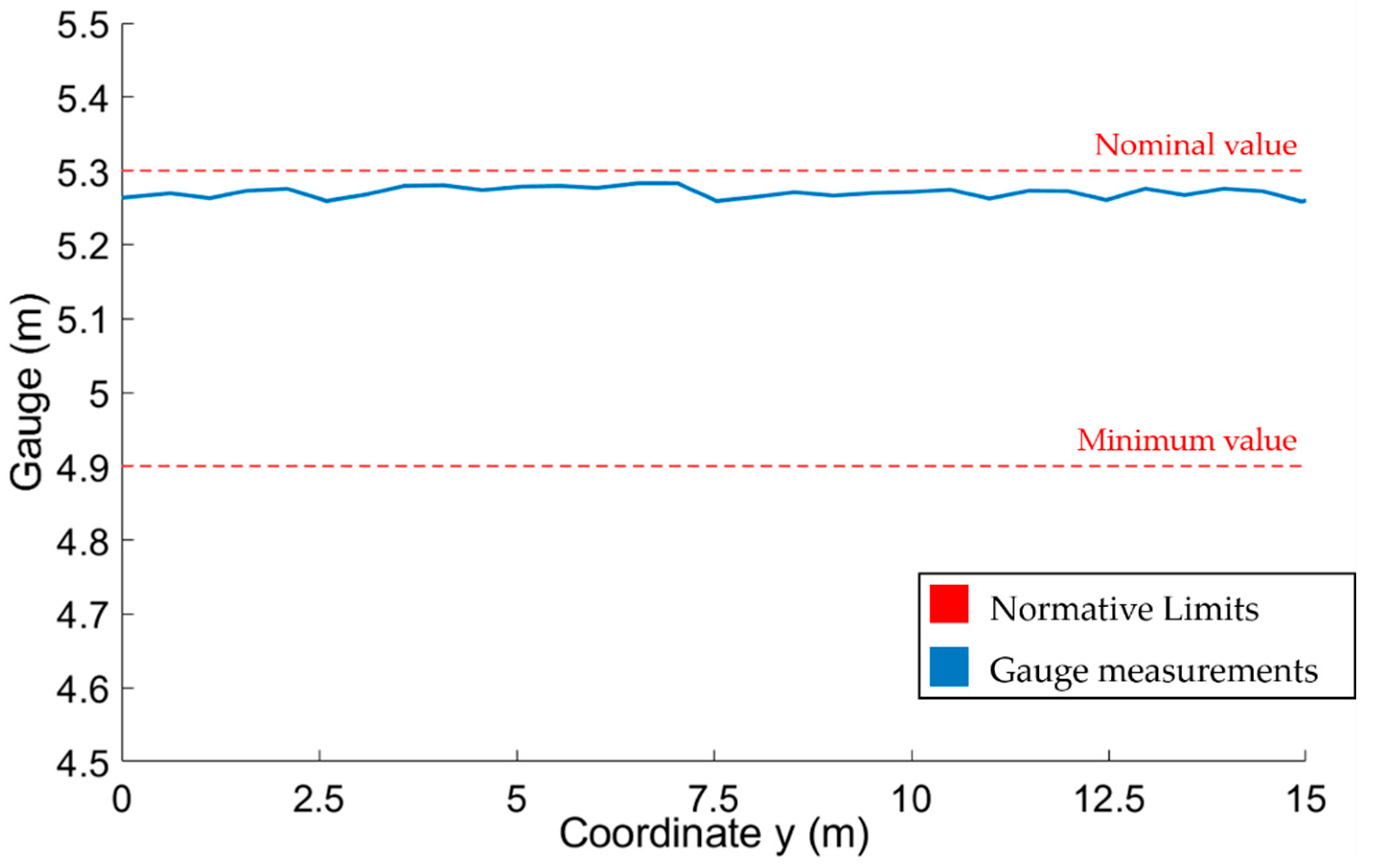
Figure 8 shows the gauge measurements, with a maximum difference of 0.0252 m. They must be within the range of 4.6 and 6 m, although the general norm is to use 5.3 m as nominal value and 4.9 as the minimum (the most restrictive one according to Table 1), as stated in ADIF’s current affairs files [2]. This is complementary with the obligation of 4.9 m as the minimum contact wire’s height in tunnels [3]. The deflection needs to be inferior than 0.853 m (Table 1), taking it as the most restrictive value for a span of 50 m, in this case. Every tunnel section studied in this work comply with this obligation and two results are presented as an example in Table 6.
From the results obtained for the one hundred sections (20-m point clouds) studied concerning gauge and deflection measurements, it can be said that the three tunnels comply with the measurement limitations of the standard summarized in Table 1.
5.4. Global Discussion
This paper proposes two different contributions concerning the work with railway tunnels’ point clouds: to evaluate the specific application of point clouds for classifying aerial contact lines; and to prove the validity of LiDAR data for performing automatic inspections of the railway network. Concerning point clouds classification (tunnel power line), a simple approach was adopted, showing high accuracies in the results. However, it is noticeable that point clouds with the lowest performance metrics belong to the suspension wires. This is caused by the difficulty for distinguishing this type of cables from the ‘fake suspension wires’ hanging by their side. Since they are too close with each other and because of their geometry, the way of labelling points in these areas is very dependent on the person manually carrying out this task. In addition, the classification results obtained were compared with the ones in the state of the art also in charge of differencing catenary and suspension wires from the rest [11,12]. In this relation, an improvement of the performance metrics is observed for both the contact and the catenary cables. Concerning the automatic inspection of the power line, none of the works in the state of the art work with point clouds in the 3D space to perform these measures.
Apart from the conclusions extracted taking into account the quantitative results in Table 5, and comparing the results with the state of the art, it can be concluded that is feasible to automatically classify aerial contact lines’ point clouds into their specific elements for a later automatic inspection.
5.5. Error Analysis
Different causes may affect the effectiveness of the proposed method, and some are subsequently presented: (i) The resolution of the available point clouds could be improved, in such a way that the number of points forming the aerial contact wire increases; (ii) some occlusions may be corrected in accordance with the previous point; and (iii) the bounding boxes established using standardized measurements could be adjusted depending on the location of the tunnels. Although the classification results presented in this section seem good, some noisy points are wrongly classified as valid, which could be avoided by improving the method as proposed.
6. Conclusions
This paper presents an automatic methodology for the inspection of two important parameters in the railway’s aerial contact line, using 3D point cloud data extracted with a mobile mapping system (MMS). The methodology is divided into three main parts, being: classification of points, distances measurement and standards’ compliance. This is considered a first approach to start defining a methodology for highlighting conflictive areas in the railway network. Conceptually, the aim of this work is to offer a preliminary method for the automation of the railway network inspection that nowadays is conducted manually and subjected to the operator’s criteria. In addition, the results presented show a good performance in terms of point cloud classification and distance measurement. It is important to highlight that there is no benchmark that allows comparing these results, so the proposed methodology has been tested under three private sets of data. This work can be considered as a proof that mobile mapping systems are valid for surveying and inspecting railway environments.
Future work may have different aspects into consideration. Working with LiDAR data, every methodology developed has room for improvement. With the trend of deep learning, the classification of points may also be done by applying specialized neural networks (PointNet, PointNet++, fpnn, splatnet, kpconv, etc.). Concerning the inspection of the aerial contact line, some other parameters are also required for a complete inspection of the line, as can be the eccentricity of the contact wire, the system’s height, the slope of the tracks, etc.
Author Contributions
Conceptualization: A.S.-R. and M.S.; methodology: A.S.-R. and M.S.; software: M.C.; validation: A.S.-R., M.S., and M.C.; formal analysis: M.C.; investigation: A.S.-R.; resources: P.A.; data curation: M.C.; writing—original draft preparation: A.S.-R.; writing—review and editing: A.S.-R., M.S., and M.C.; visualization: M.C.; supervision: P.A.; project administration: P.A.; funding acquisition: P.A.
Funding
This work has been partially supported by University of Vigo through the grant Axudas Predoutorais para a formación de Doutores 2018 (grant number 00VI 131H 6410211). This project has received funding from the European Union’s Horizon 2020 research and innovation programme under grant agreement no. 769255.
Acknowledgments
Neither of the funding bodies, the Innovation and Networks Executive Agency (INEA), nor the European Commission is in any way responsible for any use that may be made of the information it contains.
Conflicts of Interest
The authors declare no conflict of interest.
References
- FaroArm®|FARO SPAIN, S.L.U. Available online: https://www.faro.com/es-es/productos/3d-manufacturing/faroarm/ (accessed on 12 August 2019).
- Adif. Ministerio de Fomento, Gobierno de España. Available online: http://www.adif.es/ (accessed on 6 February 2019).
- Gil Calvo, M.A.; Jiménez Cano, A.; Estévez Cárdenas, F. Línea Aérea de Contacto unificado para Catenarias CA-160 y CA-220, 2nd ed.; ADIF: Madrid, Spain, 2008. [Google Scholar]
- Arastounia, M. An Enhanced Algorithm for Concurrent Recognition of Rail Tracks and Power Cables from Terrestrial and Airborne LiDAR Point Clouds. Infrastructures 2017, 2, 8. [Google Scholar] [CrossRef]
- Soni, A.; Robson, S.; Gleeson, B. Extracting Rail Track Geometry from Static Terrestrial Laser Scans for Monitoring Purposes. ISPRS—Int. Arch. Photogramm. Remote Sens. Spat. Inf. Sci. 2014, XL–5, 553–557. [Google Scholar] [CrossRef]
- Collin, B.; Carreaud, P.; Lançon, H. High Efficiency Techniques for the Assessment of Railways Infrastructures and Buildings. In Proceedings of the Transportation Research Procedia, Shanghai, China, 10–15 July 2016; pp. 1865–1874. [Google Scholar]
- Soilán, M.; Sánchez-Rodríguez, A.; del Río-Barral, P.; Perez-Collazo, C.; Arias, P.; Riveiro, B. Review of Laser Scanning Technologies and Their Applications for Road and Railway Infrastructure Monitoring. Infrastructures 2019, 4, 58. [Google Scholar] [CrossRef]
- Che, E.; Jung, J.; Olsen, M.J. Object recognition, segmentation, and classification of mobile laser scanning point clouds: A state of the art review. Sensors 2019, 19, 810. [Google Scholar] [CrossRef] [PubMed]
- Leslar, M.; Perry, G.; McNease, K. Using mobile lidar to survey a railway line for asset inventory. In Proceedings of the American Society for Photogrammetry and Remote Sensing Annual Conference 2010: Opportunities for Emerging Geospatial Technologies, San Diego, CA, USA, 26–30 April 2010; pp. 526–533. [Google Scholar]
- Arastounia, M. Automatic Classification of LiDAR Point Clouds in A Railway Environment; University of Twente Faculty of Geo-Information and Earth Observation: Enschede, The Netherlands, 2012. [Google Scholar]
- Arastounia, M. Automated Recognition of Railroad Infrastructure in Rural Areas from LIDAR Data. Remote Sens. 2015, 7, 14916–14938. [Google Scholar] [CrossRef] [Green Version]
- Arastounia, M.; Elberink, S.O. Application of Template Matching for Improving Classification of Urban Railroad Point Clouds. Sensors 2016, 16, 2112. [Google Scholar] [CrossRef] [PubMed]
- Pastucha, E. Catenary System Detection, Localization and Classification Using Mobile Scanning Data. Remote Sens. 2016, 8, 801. [Google Scholar] [CrossRef]
- Zhang, S.; Wang, C.; Yang, Z.; Chen, Y.; Li, J. Automatic railway power line extraction using mobile laser scanning data. In Proceedings of the International Archives of the Photogrammetry, Remote Sensing and Spatial Information Sciences—ISPRS Archives, Prague, Czech, 12–19 July 2016; pp. 615–619. [Google Scholar]
- Guo, B.; Li, Q.; Huang, X.; Wang, C. An Improved Method for Power-Line Reconstruction from Point Cloud Data. Remote Sens. 2016, 8, 36. [Google Scholar] [CrossRef]
- Wang, Y.; Chen, Q.; Liu, L.; Li, K. A Hierarchical unsupervised method for power line classification from airborne LiDAR data. Int. J. Digit. Earth 2018, 1–17. [Google Scholar] [CrossRef]
- Blug, A.; Baulig, C.; Wolfelschneider, H.; Hofler, H. Fast fiber coupled clearance profile scanner using real time 3D data processing with automatic rail detection. In Proceedings of the IEEE Intelligent Vehicles Symposium, Parma, Italy, 14–17 June 2004; pp. 658–663. [Google Scholar]
- Mikrut, S.; Kohut, P.; Pyka, K.; Tokarczyk, R.; Barszcz, T.; Uhl, T. Mobile Laser Scanning Systems for Measuring the Clearance Gauge of Railways: State of Play, Testing and Outlook. Sensors 2016, 16, 683. [Google Scholar] [CrossRef] [PubMed]
- Luo, C.; Jwa, Y.; Sohn, G. Context based multiple railway object recognition from mobile laser scanning data. Int. Geosci. Remote Sens. Symp. 2014, 3602–3605. [Google Scholar]
- Sánchez-Rodríguez, A.; Riveiro, B.; Soilán, M.; González-deSantos, L.M. Automated detection and decomposition of railway tunnels from Mobile Laser Scanning Datasets. Autom. Constr. 2018, 96, 171–179. [Google Scholar] [CrossRef]
- Qi, C.R.; Su, H.; Mo, K.; Guibas, L.J. PointNet: Deep Learning on Point Sets for 3D Classification and Segmentation. IEEE Conf. Comput. Vis. Pattern Recognit. 2016, 601–610. [Google Scholar]
- Qi, C.R.; Yi, L.; Su, H.; Guibas, L.J. PointNet++: Deep Hierarchical Feature Learning on Point Sets in a Metric Space. In Proceedings of the Neural Information Processing Systems, Long Beach, CA, USA, 4–9 December 2017. [Google Scholar]
- Tatarchenko, M.; Dosovitskiy, A.; Brox, T. Octree Generating Networks: Efficient Convolutional Architectures for High-Resolution 3D Outputs. In Proceedings of the IEEE International Conference on Computer Vision, Venice, Italy, 22–29 October 2017. [Google Scholar]
- Su, H.; Jampani, V.; Sun, D.; Maji, S.; Kalogerakis, E.; Yang, M.H.; Kautz, J. SPLATNet: Sparse Lattice Networks for Point Cloud Processing. In Proceedings of the IEEE Computer Society Conference on Computer Vision and Pattern Recognition, Salt Lake City, UT, USA, 18–22 June 2018. [Google Scholar]
- Balado, J.; Arias, P.; Díaz-Vilariño, L.; González-Desantos, L.M. Automatic CORINE land cover classification from airborne LIDAR data. Procedia Comput. Sci. 2018, 126, 186–194. [Google Scholar] [CrossRef]
- Balado, J.; Martínez-sánchez, J.; Arias, P.; Novo, A. Road Environment Semantic Segmentation with Deep Learning from MLS Point Cloud Data. Sensors 2019, 19, 3466. [Google Scholar] [CrossRef] [PubMed]
- Luo, Z.; Li, J.; Xiao, Z.; Mou, Z.G.; Cai, X.; Wang, C. Learning high-level features by fusing multi-view representation of MLS point clouds for 3D object recognition in road environments. ISPRS J. Photogramm. Remote Sens. 2019, 150, 44–58. [Google Scholar] [CrossRef]
- Kumar, B.; Pandey, G.; Lohani, B.; Misra, S.C. A multi-faceted CNN architecture for automatic classification of mobile LiDAR data and an algorithm to reproduce point cloud samples for enhanced training. ISPRS J. Photogramm. Remote Sens. 2019, 147, 80–89. [Google Scholar] [CrossRef]
- Hemández Puertas, J. Cálculo de Esfuerzos y Desplazamientos sobre Pórticos CA-220 con Matlab; Universidad Pontificia Comillas: Madrid, Spain, 2016. [Google Scholar]
- Soilán, M.; Riveiro, B.; Martínez-Sánchez, J.; Arias, P. Traffic sign detection in MLS acquired point clouds for geometric and image-based semantic inventory. ISPRS J. Photogramm. Remote Sens. 2016, 114, 92–101. [Google Scholar] [CrossRef]
- MathWorks-Makers of MATLAB and Simulink. Available online: https://es.mathworks.com/ (accessed on 17 Januarey 2018).
- Teledyne Optech © Teledyne Optech. Available online: http://www.teledyneoptech.com/en/home/ (accessed on 11 June 2019).
- Puente, I.; González-Jorge, H.; Riveiro, B.; Arias, P. Accuracy verification of the Lynx Mobile Mapper system. Opt. Laser Technol. 2013, 45, 578–586. [Google Scholar] [CrossRef]
- Díaz, O. Understanding Accuracy in Laser Scanners|SmartGeoMetrics. Available online: http://www.smartgeometrics.com/2013/08/28/understanding-accuracy-in-laser-scanners-2/ (accessed on 30 January 2019).
- RIEGL—RIEGL Laser Measurement Systems. Available online: http://www.riegl.com/ (accessed on 1 November 2019).
- Filgueira, A.; González-Jorge, H.; Lagüela, S.; Díaz-Vilariño, L.; Arias, P. Quantifying the influence of rain in LiDAR performance. Meas. J. Int. Meas. Confed. 2017, 95, 143–148. [Google Scholar] [CrossRef]
Figure 1.
Tunnel point cloud classification (preliminary).

Figure 2.
Flow diagram of the aerial contact line classification method.

Figure 3.
Suspension wire detection (schema).

Figure 4.
Schema of the distances to be measured.

Figure 5.
Flow diagram of the distances measurement procedure. (a) Gauge; (b) deflection.

Figure 6.
Fitted line and cantilevers: Example.

Figure 7.
Power line system, example: Tunnel A, Section 10. (a) Original cloud; (b) classification results.
Figure 7.
Power line system, example: Tunnel A, Section 10. (a) Original cloud; (b) classification results.

Figure 8.
Gauge measurements, example: Tunnel A.


Table 1.
Most used catenary models in Spain [3].
Table 1.
Most used catenary models in Spain [3].
| Characteristic | Wire Type | Catenary Model | |
|---|---|---|---|
| CA-160 | CA-220 | ||
| Section | Suspension | Cu 150 mm2 | Cu 185 mm2 |
| Contact | 2× Cu 107 mm2 | 2× Cu-Ag 0.1–150 mm2 | |
| Nominal height | Contact | 5.30 m | 5.30 m |
| System | 1.4 m | 1.4 m | |
| Minimum height | Contact | 4.60 m | 4.90 m |
| Maximum Span | Suspension | 60 m | 60 m |
| Maximum deflection 1 | Suspension | 0.853 m | 0.853 m |
1 Inside railway tunnels.
Table 2.
Acquisition parameters for Lynx Mobile Mapper [32].
Table 2.
Acquisition parameters for Lynx Mobile Mapper [32].
| Manufacturer | LiDAR Model | Maximum Range | Range Precision | PRF (Pulse Repetition Frequency) | Scan Frequency | Field of View |
|---|---|---|---|---|---|---|
| Teledyne Optech | Lynx M1 | 200 m | 8 mm | 75–500 kHz | 80–200 Hz | 360° |
Table 3.
Case study data.
| Dataset | No. of Sections (20 m Long) | No. of Points | Longitudinal Length (m) |
|---|---|---|---|
| Tunnel A | 42 | 332,646,619 | 877 |
| Tunnel B | 54 | 168,437,020 | 1151 |
| Tunnel C | 4 | 45,788,061 | 51.3 |
Table 4.
Sections selected for classification.
| Tunnel | Dataset Number | No. of Points (Total) | No. of Points (Power Line 1) |
|---|---|---|---|
| A | 10 | 7,241,901 | 36,516 |
| B | 11 | 2,955,005 | 12,146 |
| C | 4 | 19,687,427 | 61,075 |
1 Without cantilevers.
Table 5.
Segmentation results and performance metrics.
| Tunnel | Element | TP | FP | FN | Precision | Recall | F-score |
|---|---|---|---|---|---|---|---|
| A | Contact wire | 2011 | 818 | 761 | 0.9609 | 0.9636 | 0.9622 |
| Suspension wire | 7269 | 411 | 379 | 0.9465 | 0.9504 | 0.9485 | |
| B | Contact wire | 6578 | 244 | 305 | 0.9642 | 0.9557 | 0.9599 |
| Suspension wire | 3053 | 220 | 193 | 0.9328 | 0.9405 | 0.9366 | |
| C | Contact wire | 26371 | 1344 | 1028 | 0.9515 | 0.9625 | 0.9570 |
| Suspension wire | 15900 | 870 | 1322 | 0.9481 | 0.9232 | 0.9355 |
Table 6.
Deflection measurements (specifically selected sections).
| Tunnel | Dataset Number | No. of Points (Suspension Wire) | Deflection (m) |
|---|---|---|---|
| A | 8-10 | 57,750 | 0.59 |
| B | 8-11 | 26,482 | 0.67 |
© 2019 by the authors. Licensee MDPI, Basel, Switzerland. This article is an open access article distributed under the terms and conditions of the Creative Commons Attribution (CC BY) license (http://creativecommons.org/licenses/by/4.0/).
Share and Cite
MDPI and ACS Style
Sánchez-Rodríguez, A.; Soilán, M.; Cabaleiro, M.; Arias, P. Automated Inspection of Railway Tunnels’ Power Line Using LiDAR Point Clouds. Remote Sens. 2019, 11, 2567. https://doi.org/10.3390/rs11212567
AMA Style
Sánchez-Rodríguez A, Soilán M, Cabaleiro M, Arias P. Automated Inspection of Railway Tunnels’ Power Line Using LiDAR Point Clouds. Remote Sensing. 2019; 11(21):2567. https://doi.org/10.3390/rs11212567
Chicago/Turabian StyleSánchez-Rodríguez, Ana, Mario Soilán, Manuel Cabaleiro, and Pedro Arias. 2019. "Automated Inspection of Railway Tunnels’ Power Line Using LiDAR Point Clouds" Remote Sensing 11, no. 21: 2567. https://doi.org/10.3390/rs11212567
Note that from the first issue of 2016, this journal uses article numbers instead of page numbers. See further details here.