Article

Detection of Pine Shoot Beetle (PSB) Stress on Pine Forests at Individual Tree Level using UAV-Based Hyperspectral Imagery and Lidar

Key Laboratory for Silviculture and Conservation of Ministry of Education, Beijing Forestry University, Beijing 100083, China
*
Author to whom correspondence should be addressed.
Remote Sens. 2019, 11(21), 2540; https://doi.org/10.3390/rs11212540
Submission received: 26 September 2019 / Revised: 25 October 2019 / Accepted: 25 October 2019 / Published: 29 October 2019
(This article belongs to the Section Forest Remote Sensing)

Abstract

:
In recent years, the outbreak of the pine shoot beetle (PSB), Tomicus spp., has caused serious shoots damage and the death of millions of trees in Yunnan pine forests in southwestern China. It is urgent to develop a convincing approach to accurately assess the shoot damage ratio (SDR) for monitoring the PSB insects at an early stage. Unmanned airborne vehicles (UAV)-based sensors, including hyperspectral imaging (HI) and lidar, have very high spatial and spectral resolutions, which are very useful to detect forest health. However, very few studies have utilized HI and lidar data to estimate SDRs and compare the predictive power for mapping PSB damage at the individual tree level. Additionally, the data fusion of HI and lidar may improve the detection accuracy, but it has not been well studied. In this study, UAV-based HI and lidar data were fused to detect PSB. We systematically evaluated the potential of a hyperspectral approach (only-HI data), a lidar approach (only-lidar data), and a combined approach (HI plus lidar data) to characterize PSB damage of individual trees using the Random Forest (RF) algorithm, separately. The most innovative point is the proposed new method to extract the three dimensional (3D) shadow distribution of each tree crown based on a lidar point cloud and the 3D radiative transfer model RAPID. The results show that: (1) for the accuracy of estimating the SDR of individual trees, the lidar approach (R2 = 0.69, RMSE = 12.28%) performed better than hyperspectral approach (R2 = 0.67, RMSE = 15.87%), and in addition, it was useful to detect dead trees with an accuracy of 70%; (2) the combined approach has the highest accuracy (R2 = 0.83, RMSE = 9.93%) for mapping PSB damage degrees; and (3) when combining HI and lidar data to predict SDRs, two variables have the most contributions, which are the leaf chlorophyll content (Cab) derived from hyperspectral data and the return intensity of the top of shaded crown (Int_Shd_top) from lidar metrics. This study confirms the high possibility to accurately predict SDRs at individual tree level if combining HI and lidar data. The 3D radiative transfer model can determine the 3D crown shadows from lidar, which is a key information to combine HI and lidar. Therefore, our study provided a guidance to combine the advantages of hyperspectral and lidar data to accurately measure the health of individual trees, enabling us to prioritize areas for forest health promotion. This method may also be used for other 3D land surfaces, like urban areas.

Graphical Abstract

1. Introduction

The disturbances of forest insects severely destroy forest health, carbon dynamics, ecosystem stability, and increase their vulnerability to natural disturbances [1,2,3,4]. In southwestern China, the Yunnan Pine forests have infested around 1.5 million hectares over the past 20 years. The most damage was attributed to the pine shoot beetle (PSB) insects (e.g., Tomicus spp.) [5]. Thus, it is urgent to develop an accurate and efficient approach to detect PSB damage for protecting forest health sustainability management.
The effective detection and monitoring of forest insects have long been a central focus in remote sensing and forest management communities [6,7,8]. Generally, forest insects can be classified into two groups including folivorous (e.g., defoliators) and xylophagous insects (e.g., woodborers) [9]. Defoliators feeding on leaves or needles have a clear damage mechanism. Numerous remote sensing-based approaches such as vegetation indices [7,10], spectral mixture analysis [11], image classification [12,13], and time series approaches [14,15] have been successfully used to map defoliation due to the defoliators infection causing obviously visible symptoms of forest cover and leaf discoloration [14]. However, woodborers (e.g., mountain pine beetle (MPB) and PSB) attack is much more vague and complex [5,16]. The MPB has an annual life cycle with four stages including egg, larva, pupa, and adult [17], which is much clearer than the PSB. Infected forests exhibit unique and visible characteristics at each stage of a MPB attack [18,19]. During the attacking, infected trees changes from green to yellow, to red, and finally to gray. At the gray attack stage, most trees lose all their needles at that time [18,19]. There are detailed field data of the MPB including aerial detection surveys and ground surveys from local agencies, such as the USDA (United States Department of Agriculture) Forest Service [19,20,21]. Therefore, remotely sensed methods have been effectively detecting and mapping MPB infestations based on the clear life cycle, obvious attack stage, and detailed field data [17,22,23,24,25].
As for PSB (Tomicus spp.), the life cycle is still unclear. The process of the Tomicus spp. attack can only be roughly divided into two stages, which are the trunk-shoot stage and the shoot-trunk stage [5]. At the trunk-shoot stage, beetles coming out of trunks attack the vigorous shoots of the Yunnan Pine. Then, at the shoot-trunk stage, there is a visible symptom of PSB attack, which is the change of needles color from green to red [5]. However, shoots discoloration symptoms may have a lag of several weeks since the initial attack. The spread mode of beetles from one tree to another is also unknown. These critical knowledge gaps make it more difficult to monitor PSB damage. There are some studies attempted to measure PSB damage using satellite data, for example, Yu et al. [5], using the indicator of shoot damage ratio (SDR) to define forest damage severity by PSB attack, and employing multi-temporal Landsat images to map PSB outbreak time and spread direction. Lin et al. [26] explored the inversion using a radiative transfer model (RTM) against Sentinel 2A imagery at 20 m spatial resolution (8 bands) for retrieval of SDRs for measuring PSB damage. However, the above mentioned satellite image-based remote sensing methods focused on stand level at the outbreak stage of PSB attack. At early stage of PSB attack, a forest stand may only contain a few infected trees, which have a diversity of health conditions with high spatial heterogeneity. The traditional mulitspectral satellite images (e.g., Landsat) were difficult to distinguish damaged tree crowns from health tree crowns at around 30 m resolution for the early stage of forest insect attack [27]. Moreover, mid- and low-resolution remote sensing data are not readily applicable for forest health studies at the individual tree level due to limitations in the capacity of satellite imagery to detect suppressed trees that were barely seen [28,29]. Especially, the slightly infected Yunan Pine trees only have several damaged shoots within crowns. It needs very high spatial and even high spectral resolution to distinguish the slight difference between healthy and damaged tree crowns. Therefore, it is urgent to develop an accurate and cost-efficient method to measure PBS damage at individual tree level for early monitoring. To our knowledge, there is no previous study on mapping PSB damage severity at individual tree level.
With the fast development of unmanned airborne vehicles (UAV) platforms and light sensors, UAV-based imaging technologies using very high resolution optical imaging spectroscopy (IS) and light detection and ranging (lidar) have great potential in forest health monitoring at individual tree level [29,30,31,32]. IS features such as hyperspectral imagery (HI) provided continuous narrowband spectral information, which greatly enhanced the capability to extract forest health information [11,33]. Lidar data, being able to retrieve detailed three dimensional (3D) information about tree canopies with a high density of laser pulses, are useful in characterizing the spatial arrangement of foliage [34,35]. In combination with the 3-D coordinates of each laser point, laser return intensity could be used for measuring the reflection characteristic in the near infrared (NIR) region and spatial arrangement of foliage in a tree crown [36,37], which provides new opportunities for monitoring forest health in the context of the detection and mapping of forest infestations [38,39,40]. However, there are some limitation on measuring individual tree health status when using HI and lidar data alone. For example, HI is difficult to accurately delineate the crown structure (especially the height), and in addition, the shadow of the tree crown causes spectral variation problems like the reduction of spectral information and change in the spectral shape [41], and should be either eliminated in HI analysis or compensated using extra data (e.g., lidar). Potentials on data combination of lidar and IS data have not been sufficiently assessed for mapping forest health at crown scale. Furthermore, many studies focused on the herbivorous insects and MPB, but very few works have been found on exploring the utility of HI or lidar data for measuring PSB damage.
Therefore, our objective is to explore the potential of integrating UAV-based lidar and HI to quantify the tree crown damage severity by PSBs. The SDR is used as an indicator for assessing tree crown damage severity by PSB attack. Furthermore, we investigated the impact of lidar and HI data information complementation for shadowed crowns on measuring PSB damage. To achieve that goal, a 3D radiative transfer model, RAPID [42], is introduced and used. By combing HI and lidar datasets, as well as corresponding field measurements, we are trying to answer the following research questions: (1) At individual tree level, what are the most sensitive spectral and structural signatures of canopies reflecting the tree crown damage severity by PSB insects? (2) What are the differences in predictive power of airborne HI and lidar data for mapping the tree crown damage severity by PSB insects? (3) Can the combined use of IS and lidar data improve mapping accuracy?

2. Materials and Methods

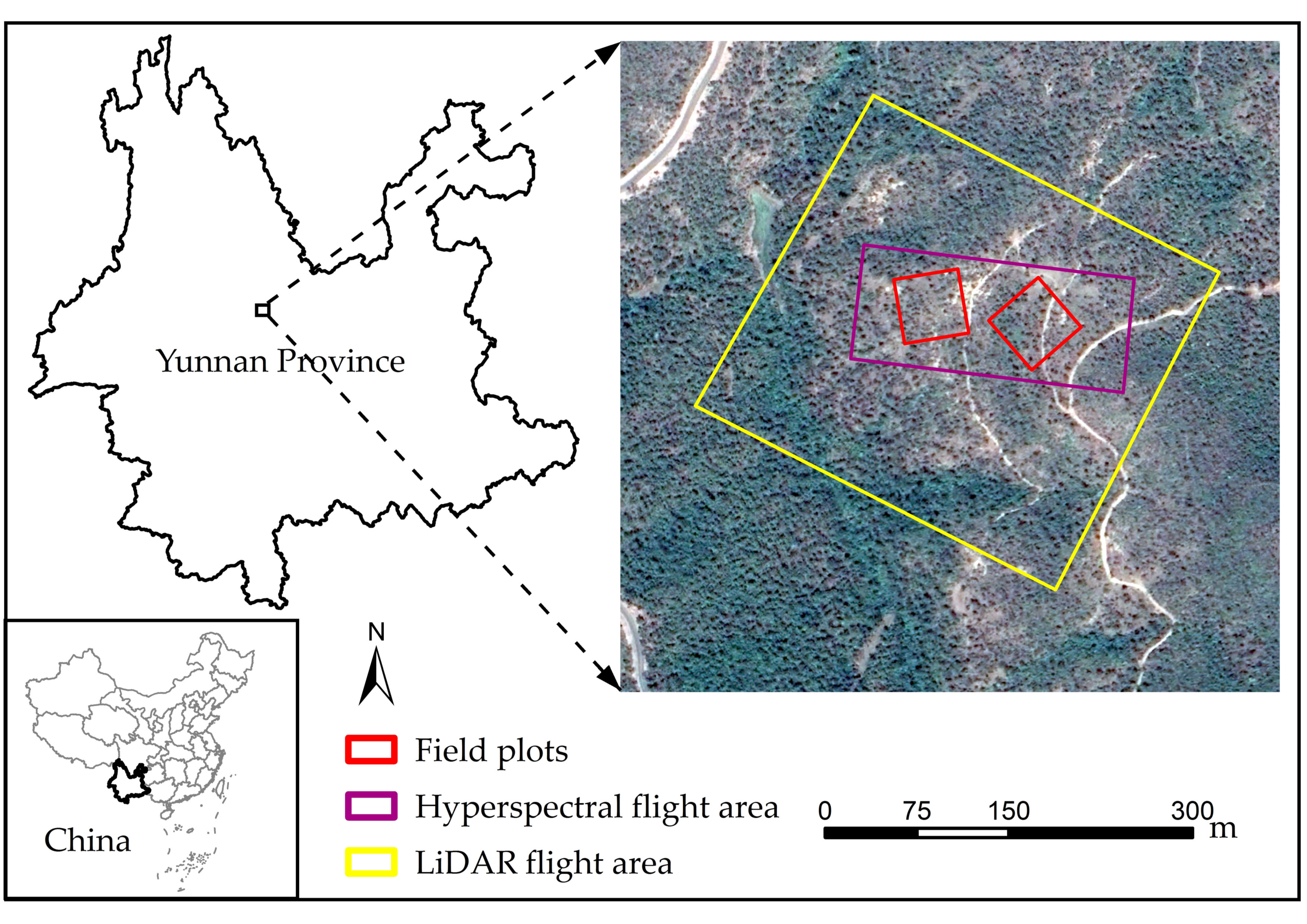
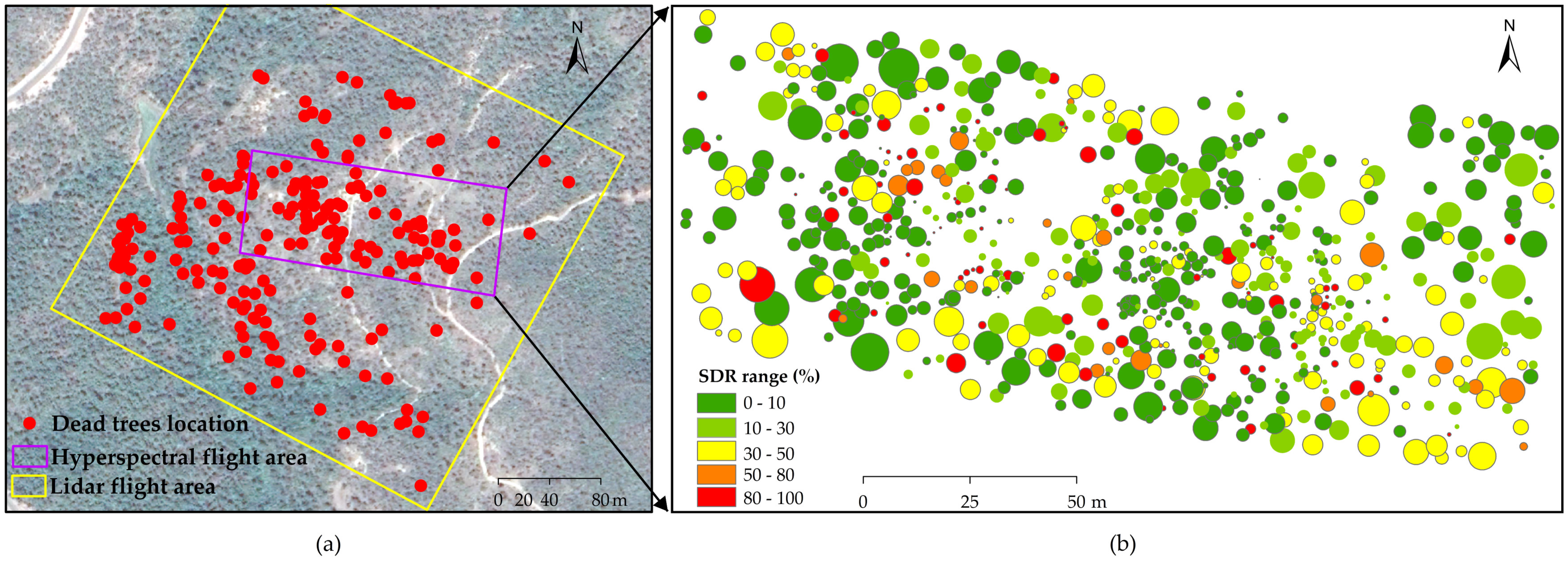
2.1. Study Area and Field Measurements

The study site (25°14′–25°29′N, 100°48′-101°3′E), is located in the Tianfeng Mountain, Yunnan Province, of southwestern China (Figure 1). In this area, the species of plantation forests is dominated by the Yunnan Pine (Pinus yunnanensis) with an area of about 1000 ha. According to the records of the local Forestry Administration, the pine shoot beetles (PSB), Tomicus spp. (including two members of Tomicus yunnanensis and Tomicus minor), boring into shoots and usually beginning at the top of tree crowns, have been causing the death of tens of thousands of pine trees since the outbreaks in 2013 [5].
Field measurements were conducted in September 2018. Two plots were set with the size of 50 m x 50 m in the area (Figure 1). The boundary coordinates of each plot and tree locations were measured using a real-time kinematic (RTK) GPS device (HI-TARGET A8 GNSS) with an accuracy of approximately ±2.5 mm. In each plot, tree variables including tree height (H), crown base height (CBH), diameter at breast height (DBH), crown diameter (CD), and SDR were measured. The SDR was defined as the proportion of damaged shoots number to total shoots number for each tree crown [5,26]. Each SDR was between 0% and 100%. We divided tree damage degrees into five levels: healthy tree (SDR: 0–10%), slightly infected tree (SDR: 10–30%), moderately infected tree (SDR: 30–50%), severely infected tree (SDR: 50–80%), and dead tree (SDR: 80–100%). Moreover, the biochemical parameters such as the leaf chlorophyll content (Cab) of single trees were derived by averaging four level shoots Cab using a calibrated CCM-300 Chlorophyll Content Meter [26]. Summary statistics of two plots are given in Table 1.

2.2. Remote Sensing Data Acquisition and Processing

2.2.1. Hyperspectral Imagery

The HI (purple rectangle in Figure 1) data were acquired using the pushbroom Nano-Hyperspec (Headwall Photonics Inc., Germany) with a vertical downward observation mode from 13:00 to 13:30 P.M., 21 September 2018. The sky was clear during the flight campaign. The HI sensor is with a field of view of 8° and a focal length of 17 mm. The imagery consisted of 270 spectral channels from visible to NIR (VNIR) regions (400–1000 nm). The flight was at a height of 70 m and the paths were designed to be at 60% across-track overlapping. Radiometric calibration and reflectance correction of all sub-imageries were performed using a 3 m2 carpet reference and the Headwall’s SpectralView software. Images geometric corrections were performed using 10 ground control points (GCPs). The positions of GCPs were measured by an RTK GPS device. The spatial resolution of HI were produced to be 0.2 m.

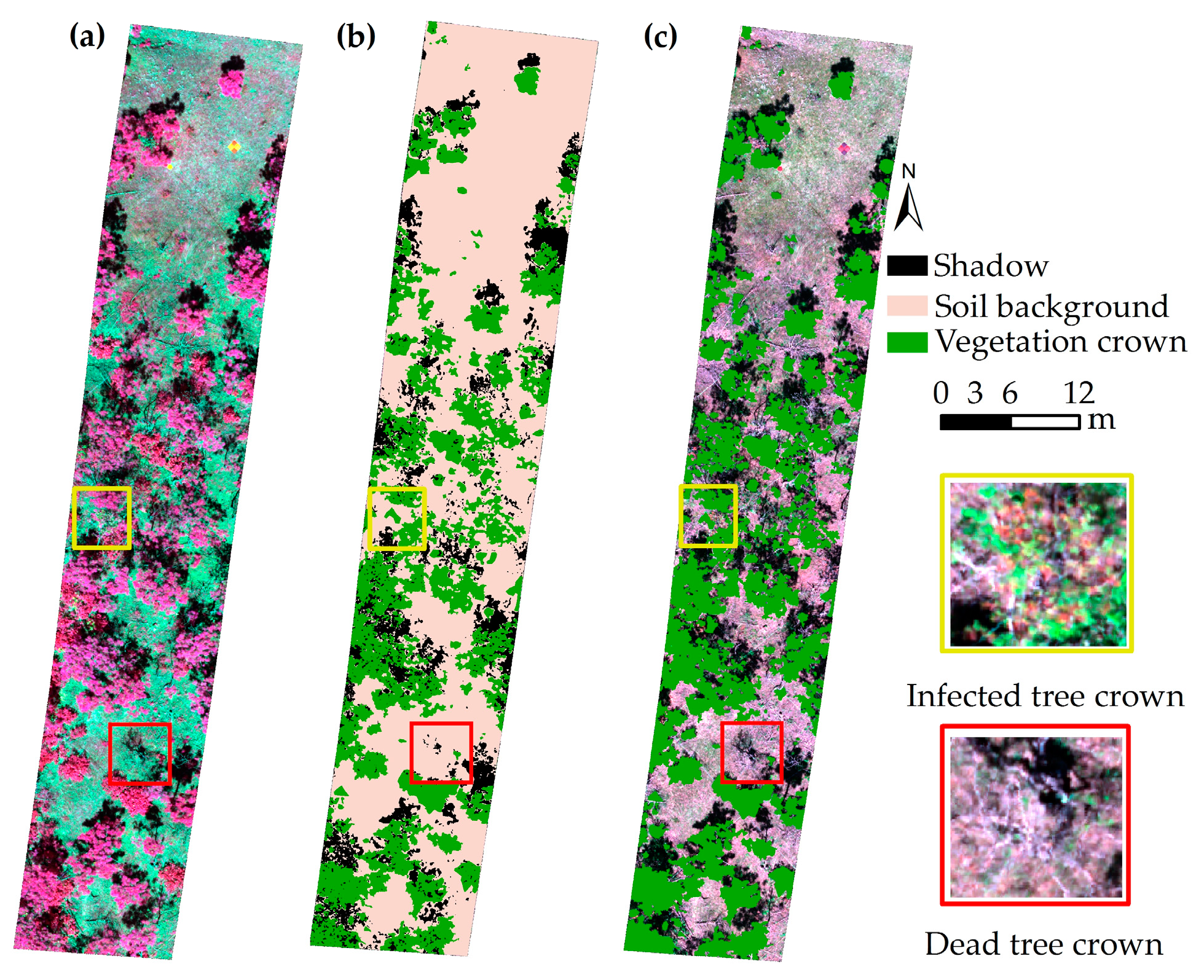
2.2.2. Tree Crowns Segmentation from Hyperspectral Imagery

The crowns segmentation from HI images were implemented in three steps. Firstly, the object-based segmentation method was applied on HI using combined spectral and texture features to separate crowns from soil background and shadows [43]. Secondly, the binary watershed analysis and the Euclidian distance were used to separate overlapping crowns [44,45]. The segmentation accuracy was assessed by the single tree detection rate (STDR), which is the ratio between detected tree crown numbers and measured true value. The object-based segmentation method successfully separated vegetation from non-vegetation (bare soil) and shadow components, but was difficult to distinguish tree from understory (Figure 2b). Furthermore, partially infected tree crown and dead (SDR = 100%) tree crown were unable to be distinguished from soil. Finally, the shadow components were discarded, and the remaining sunlit crowns were selected (Figure 2c) for further analysis. As a result, a total of 215 trees were segmented with an STDR of 48.0% for HI segmentation.

2.2.3. Lidar Data

UAV-lidar data in the same region (yellow rectangle in Figure 1) were collected on 4 September 2018, using the LiAir 200 UAV-mounted system (GreenValley Inc., China) with integrates a 40-channel Pandar40 laser sensor. The flight campaign operated at a mean flight altitude of 70 m above ground level, with a laser pulse rate of 10HZ, a maximum 10°off-nadir viewing angle (from 2-channel to 30-channel). The point density ranges from 200 to 1000 points per m2. Lidar data were georeferenced in the Universal Transverse Mercator (UTM) 50N and coordinate system is based on the WGS84 datum. The improved progressive TIN densification (IPTD) algorithm [46] was applied to classify the raw lidar point data into ground and above-ground points, which was conducted by the lidar360 software (GreenValley Inc., China). The 0.5 m raster products, including digital elevation model (DEM), digital surface model (DSM) and canopy height model (CHM) were derived from the classified point cloud. The normalized lidar data were then derived using the DEM product.

2.2.4. Individual Tree Segmentation from Lidar

A point cloud segmentation (PCS) algorithm [47] from the top-down way was adopted to separate tree crowns. PCS treated the seed points as the tree top in a point cluster (the global highest point), which can be derived from CHM with a watershed algorithm. The points below the tree top were sequentially classified to a nearest tree using a spacing threshold rule. When all trees have been segmented, the tree locations, heights, crown areas, and crown volumes were estimated from the individual tree point cloud. As for lidar segmentation, a total of 395 trees were segmented with an STDR of 88.2%.

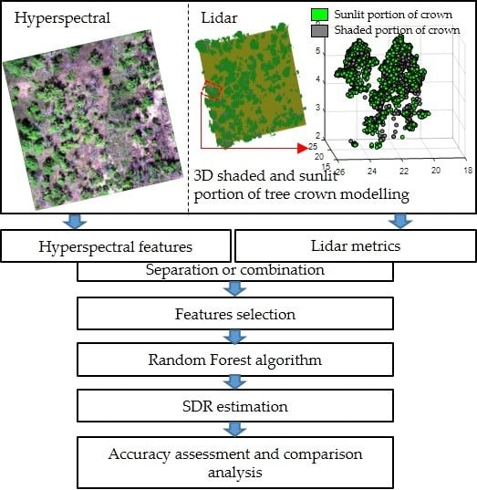
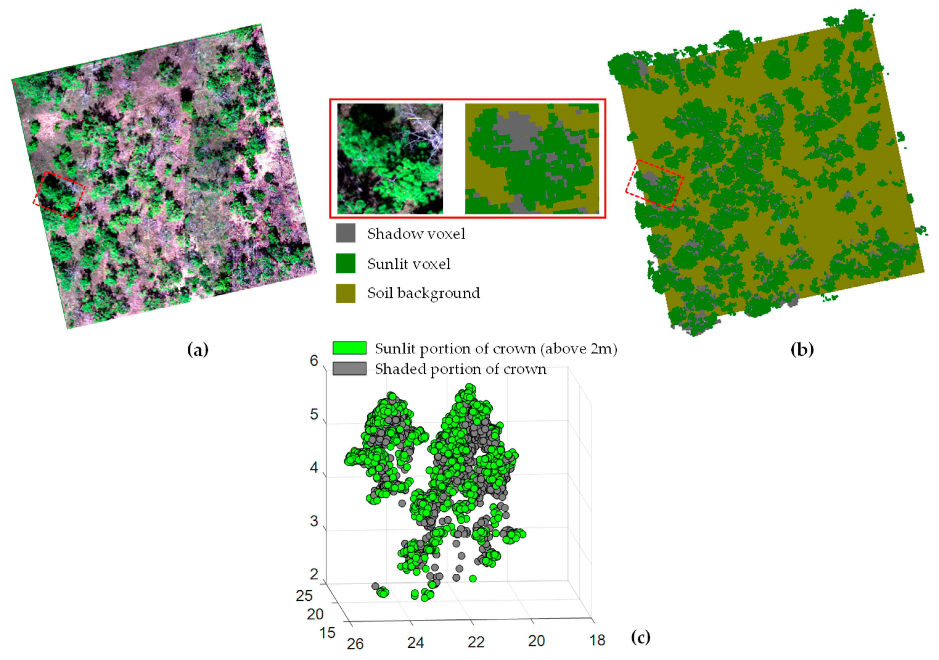
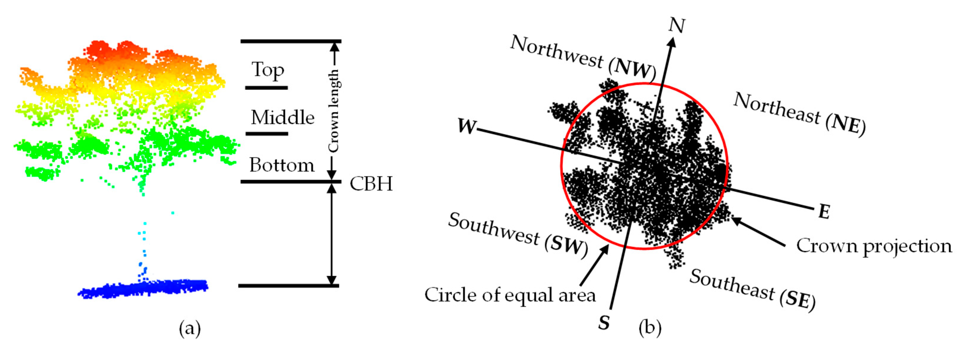
2.2.5. 3D Shaded and Sunlit Portions of Tree Crown Modelling

Optical images only measure the 2D (or horizontal) information of crowns in one observation direction. High density lidar pulses can accurately measure the 3D geometric (horizontal plus vertical) information of forest canopies. Therefore, the integration of lidar data into HI analysis could provide critical information on the shadow distribution of a tree crown [29]. The lighting conditions in tree crown pixels of HI were determined using a combination of lidar point cloud and solar geometry at the acquisition time of HI [29]. Three dimensional RTMs can be used to simulate the light conditions of tree crowns for a forest scene structure (created by lidar data). In this study, we only considered intra-canopy mutual shadowing. To model 3D sunlit or shaded portions of tree crowns, we proposed a new method as below:
(1) Voxelization:
All segmented lidar point cloud data were converted into voxels. The 0.3 m was considered as the most suitable voxel size, which simplifies the lidar point data, and effectively depicts shoots distribution within a crown and crown envelope [48].
(2) Estimation of transmission rate and leaf area density (LAD):
We assume that each lidar pulse travels near vertically due to a narrow range off-nadir viewing angle and low flight altitude. Within each 0.3 × 0.3 × 0.3 m3 voxel, the transmission rate could be estimated by counting the number of lidar pulses that enter (pulse.in) and pass through (pulse.out) it in a given vertical column, and LAD was calculated using the MacArthur–Horn equation [49]:
L A D i = ln ( p u l s e . i n p u l s e . o u t ) 1 k Δ z
where Δz is the vertical resolution (set at a constant value 1 m), and k is an adjustment factor that represents a Beer–Lambert Law extinction coefficient. We fixed k = 1 with reference to the previous study [50]. Finally, the empty and occluded (pulse.in = 0 or pulse.out = 0) voxels were removed.
(3) Construction of 3D forest scene and simulation of direct light cast fraction (fdirect):
A computer graphics method based on line-of-sight analysis was used to determine whether the tree crowns were illuminated or not in a forest scene. The 3D RTM model Radiosity Applicable to Porous IndiviDual objects (RAPID) [42] was used in this study. It uses many parallel porous objects to represent the tree crowns. The tree crowns were voxelized as many 0.3 × 0.3 × 0.3 m3 voxels. Each voxel is a porous object with several properties including length (0.3 m), thickness (0.3 m), transmission rate, and LAD. The porous objects above 2 m height (the understory was ignored) were used to generate a 3D forest scene for RAPID (Figure 3b). Since we only need the shadow distribution, we only executed the direct light simulation. The direct light cast fraction (fdirect) represents the ratio of sunlit pixel number to all-facet pixel number for each porous object. The fdirect of each porous object was simulated at a given solar and viewing angle within the 3D forest scene. In this study, the porous objects with fdirect less than 0.4 were regarded as shadow objects. That means the corresponding point cloud voxels are also shadowed, thus defined as the shaded portion of tree crowns (Figure 3). The threshold of fdirect effect was addressed in detail in the discussion section.

2.3. Features Extraction

2.3.1. Hyperspectral Features Extraction

Due to issues such as the shadow of tree crowns, it has often been advantageous to use only sunlit pixels for vegetation functional traits retrieval [51,52]. For each segmented tree crown, the sunlit pixels of crowns were selected for further analysis. A principal component analysis (PCA) was applied to reduce the data dimensionality of HI for each crown. Two principal components with the cumulative proportion of 97% were derived. In addition, we computed two groups of hyperspectral indices including normalized differential vegetation indices (NDVI), and leaf pigment activity related indices (such as: chlorophyll and anthocyanin) from the VNIR (400–1000 nm) region within each crown based on previous research.

2.3.2. Lidar Metrics Extraction

After individual tree crowns were segmented, lidar metrics depicting the spatial structure signatures of tree crowns were derived. According to [53], lidar metrics could be classified into two groups: geometric metrics (e.g., tree height, crown shape, and crown transparency) and radiometric metrics (e.g., laser return intensity). Based on the geometric metrics presented by [36,54], we calculated five metrics, including tree height, proportion of crown length to tree height, ratio between crown length to crown diameter, crown density within a circle (shown in Figure 4b) with area equal to the tree crown cover, and gap fraction. For radiometric metrics, we selected the variables based on laser return intensity, including the mean, numbers, skewness, standard deviation, coefficient of variation, nth (i.e., 25th, 50th, and 75th) percentile and cumulative percentile of laser return intensity from first or all return points of tree crowns with height above 0.5 m. In addition, we considered the distribution of damaged shoots within the tree crowns. The spatial arrangement of the tree crowns were divided into four horizontal directions (Northeast (NE), Northwest (NW), Southwest (SW), and Southeast (SE)) and three vertical heights (top, middle, and bottom) (Figure 4). Besides, the shadow fractions of the tree crowns in different vertical levels were calculated. Finally, the variables of laser return intensity were derived from different spatial arrangement and shaded portions of each tree crown.

2.3.3. Retrieval of Leaf Chlorophyll Content (Cab) from Hyperspectral Images

RTMs inversion is considered as an accurate and robust method to retrieve biophysical parameters from Earth observation data [55,56]. According to previous studies [52,57], RTMs also can be used for structural and chemical properties retrieval for individual tree crowns. Thus, the leaf biochemical (e.g., Cab) and canopy biophysical parameters were retrieved by inverting two coupled physically-based RTMs using the Lookup-table (LUT)-based method.
In this study, the widely used PROSAIL [58], linking leaf-optical model PROSPECT [59] and 4SAIL [60] canopy reflectance model, was used in a forward mode to generate the LUT. We selected the latest version PROSPECT-D [61] to update PROSAIL because it completely considered multiple plant pigments and has good accuracy in simulating realistic leaf optical properties for different physiological conditions of leaf. It is suitable for simulating the optical properties of stressed leaves.
A LUT containing 1375000 simulations was generated from the uniform distribution of input parameter combinations. The range of leaf chlorophyll (Cab) and leaf area index (LAI) were defined from field data, while soil reflectance, viewing geometry and solar zenith angle were extracted from the hyperspectral image metadata. Others parameters (shown in Table 2) include, leaf mass per area (Cm), equivalent water thickness (Cw), leaf structure parameter (N), carotenoid content (Car), anthocyanin content (Canth), average leaf angle (ALA), and hot spot size were set according to the similar literature [45,52,62]. The parametrization of the LUT was based on the input parameters and range described in Table 2.
Because PROSAIL simulates homogeneous canopies, we only used the spectral information of selected sunlit pixels to minimize the shadow influences [45,52]. In the process of LUT-based inversion, Cab was estimated by comparing the simulated spectra and UAV canopy spectra using root mean square error (RMSE) as the cost function, and each Cab estimation was based on the average of the 3000 closest matching LUT entries.
R M S E = i = 1 n ( R m e a s u r e d λ R L U T λ ) n
where Rmeasured λ is a measured canopy reflectance at wavelength λ; RLUT λ is the simulated canopy reflectance at wavelength λ in the LUT; and n is the number of wavelength.

2.4. Features Selection and Prediction Model for SDR

A Random Forest (RF) [63] regression model, using a bagging method based on the CART regression tree, was used to estimate SDR. In the RF regression, each tree was built using a deterministic algorithm by selecting a random set of variables and a random sample from the training dataset (i.e., the calibration data set) [64]. In the RF algorithm, the mean decrease accuracy (MDA) index of each variable is determined during the out-of-bag (OOB) error calculation. OOB error produces a measure of the importance of the variables by comparing how much OOB error of estimate increases when a variable is excluded and others are left unchanged [65,66,67]. Therefore, the higher MDA values of a variable is, the more importance it is [36,52,68]. Before these variables were chosen for building a regression model to predict tree crown SDR, the stepwise regression method was applied with a 95% level of confidence (p < 0.05) to test the multicollinearity between variables and eliminate the unnecessary variables. Finally, a total of 25 variables including 11 hyperspectral features (including Cab and 10 hyperspectral indices) (Table 3) and 14 lidar metrics (Table 4) were selected for SDR estimation.
To compare the predictive capabilities of HI and lidar data for mapping SDR using the RF regression model at the crown scale, there are three predicted approaches:
(1)
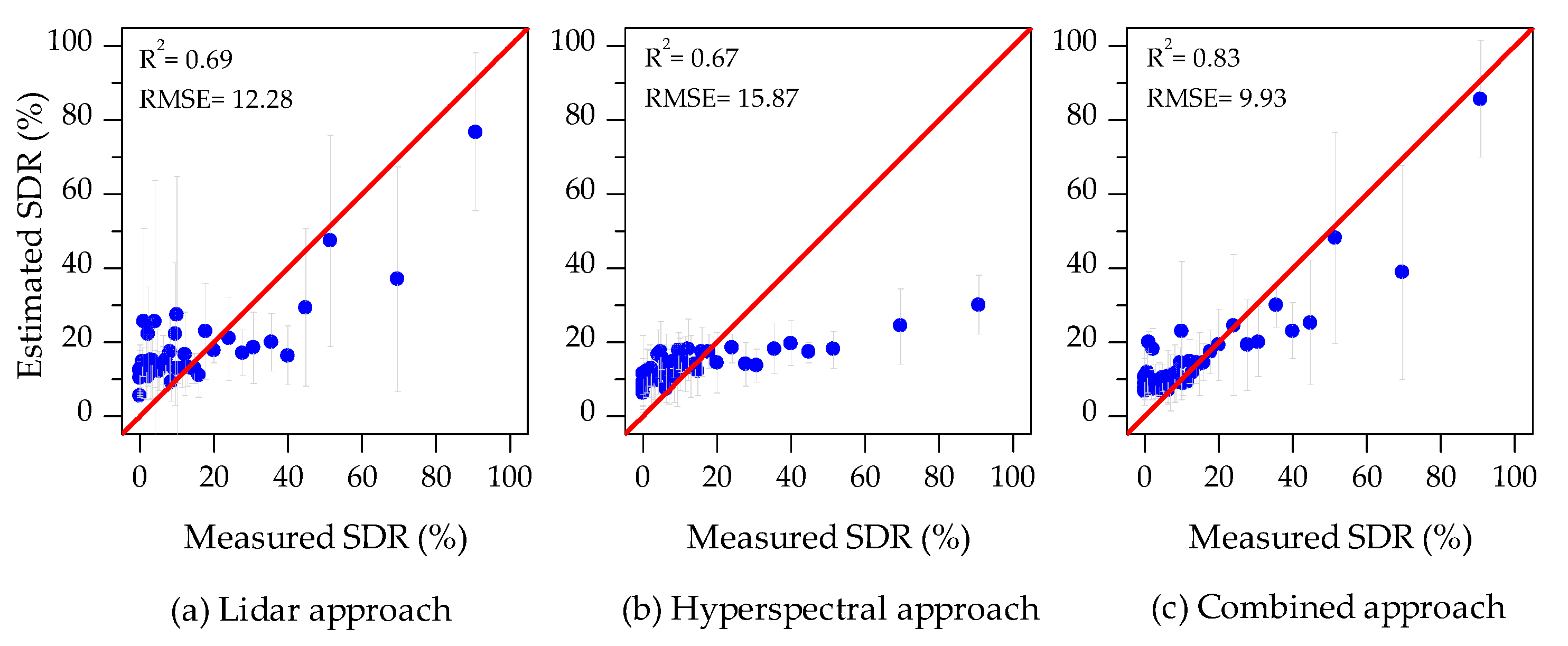
Hyperspectral approach (using only-HI variables for prediction): the tree crowns were segmented only using HI data; then 11 hyperspectral indices and Cab were derived from the selected sunlit pixels within each tree crown. Finally, 11 hyperspectral features were chosen for estimating SDR.
(2)
Lidar approach (using only-lidar variable for prediction): The trees crown were segmented using lidar data. Then, 14 lidar metrics were chosen for estimating the SDR for each tree crown.
(3)
Combined approach (using both HI and lidar variables): the crown delineation from lidar segmentation was used for hyperspectral images. For each tree crown, both lidar metrics and hyperspectral features were derived. A combination of 11 hyperspectral features and 14 lidar metrics were chosen for estimating the SDR.
Because the detected trees using lidar or HI were different, only the intersections of the segmented tree crowns (215 samples) were used for comparisons among the three approaches. For each approach, the RF regression was applied using a maximum of 1000 decision trees and a minimum OOB error to select the best regression model. All the 215 samples were used for RF regression model training, and a 10-fold cross-validation method was used for model accuracy assessment. The regression procedure was implemented using the R package “randomForest” [69]. The coefficient of determination (R2) and RMSE between measured and estimated values, as well as the STDR, were used to compare different approaches in mapping the SDR accuracy. To further assess the additional accuracy contribution of lidar on the dead trees mapping, 395 trees from lidar segmentation were used to compare the lidar and combined approaches by repeating the RF regression process again.

3. Results

3.1. Inversion Results of Tree Crown Cab

Figure 5 shows the performance of Cab retrieval from the tree crowns using different individual tree crown segmentation from HI and lidar data, respectively. The accuracy of Cab retrieval using tree crown segmentation from lidar data (R2 = 0.89, RMSE = 6.03 ug/cm2) was better than using tree crown segmentation from HI (R2 = 0.54, RMSE = 8.92 ug/cm2). Figure 5a shows that Cab below 30 ug/cm2 was mostly overestimated. This result demonstrates the evidence of impossibility detection Cab lower than 30 ug/cm2 if only using hyperspectral data at single tree level. Additionally, Figure 5b shows that Cab below 30 ug/cm2 also performed not good enough, although the tree crown delineation from lidar segmentation was used. It means that inversion of 1-D PROSAIL model was still difficult to accurately extract Cab for damaged tree crowns.

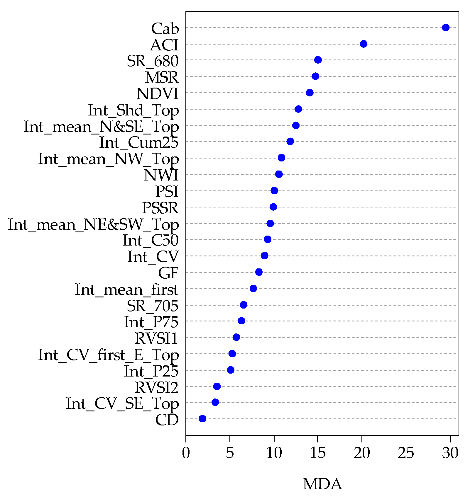
3.2. Features Selection

Figure 6 shows the average reflectance curves of different damage levels of the SDR of trees crowns from 400 to 1000 nm. As expected, the reflectance of trees crown was decreasing with the increasing of the SDR. Among the different damage levels of SDR, the differences in spectral reflectance were most evident in the red edge (660–750 nm), NIR shoulder, and plateau (750–1000 nm).
The responses of a number of hyperspectral variables and lidar metrics to SDR were shown in Figure 7. The hyperspectral indices such as MSR values significantly decreased with the increasing of the SDR. However, ACI and NWI increased with the increasing of the SDR. Almost all lidar metrics showed small change for the slight to severe infection trees. It indicated that lidar metrics were practically impossible to detect the SDR for the damaged trees (SDR < 80%). However, the dead trees (SDR ≥ 80%) showed significant differences from other damage levels for each lidar metrics. In brief, the hyperspectral variables were more sensitive than lidar metrics to the biochemical and biophysical characteristic change for different damage trees.

3.3. Estimation of Shoot Damaged Ratio (SDR)

Figure 8 shows the comparison of the tree crown SDR estimation accuracy using different methods, including the hyperspectral approach, lidar approach, and combined approach. The corresponding STDRs are 88.2%, 48.0%, and 88.2%, separately. The tree crown SDR prediction using the lidar approach (R2 = 0.69, RMSE = 12.28%) performed better than using the hyperspectral approach (R2 = 0.67, RMSE = 15.87%). However, the tree crown SDR greater than 30% was underestimated in hyperspectral approach. The best results (R2 = 0.83, RMSE = 9.93%) of tree crown SDR estimation was from the combined approach using both hyperspectral variables and lidar metrics. But for the lidar and combined approaches, the standard deviation (SD) of SDR estimations are larger than hyperspectral approach for the damaged trees with a SDR larger than 40%.
Table 5 shows the comparison results of the accuracies at different levels of tree damage for lidar and combined approaches (395 samples). The combined approach (R2 = 0.90, RMSE = 9.16%) performed better than lidar approach (R2 = 0.81, RMSE = 14.20%) for mapping the damaged degree of trees at crown scale due to the contribution of hyperspectral variables. For either the combined approach or lidar approach, the predictions on slightly infected trees and dead trees performed better than those of moderately to severely infected trees. For the lidar approach, the best performance of SDR estimation is with an accuracy of 70%, which was obtained for the dead trees. It means that lidar data have a good ability to detect dead tree crowns caused by PSB insects.
Figure 9 shows the importance rankings of 25 features from the RF regression using the MDA index for the combined approach. It can be understood that Cab and spectral indices play greater importance than most lidar metrics. Thus, the five most importance variables are from hyperspectral variables; while there are still ten of the top 20 variables from the lidar metrics. In these lidar metrics, the laser intensities have better importance than the structure variables for SDR estimation. Specifically, Int_Shd_top and Cab were the two top important variables of lidar and hyperspectral data, respectively.

3.4. Shoot Damaged Ratio (SDR) Mapping

Figure 10 shows the best mapping results of dead trees and SDRs. The trained RF regression model using combined hyperspectral variables and lidar metrics was used for the SDR mapping. In addition, the dead trees (SDR ≥ 80%) and their locations were mapped employing the lidar approach (red symbols in Figure 10a) in lidar flight area (yellow rectangle). Figure 10b shows the result of individual tree crown segmentation and SDR mapping using the combined approach in the hyperspectral flight area (purple rectangle in Figure 10a).

4. Discussion

In this study, we employed three approaches including the hyperspectral approach (using only-HI data), lidar approach (using only-lidar data), and combined approach (using both lidar and HI data), to evaluate the capacity of airborne hyperspectral and lidar remote sensing data in SDR estimation at individual tree level. The results reveal that the combined approach yielded an improved SDR estimation, with RMSE of 9.93% compared to the lidar approach (RMSE = 12.28%) or hyperspectral approach (RMSE = 15.87%). Specifically, the combined approach has good performance (the accuracy larger than 65%) to predict SDRs when tree crown SDRs ranged from 0 to 30% or 80% to 100% (Table 5).
The hyperspectral variables (Table 3) and lidar metrics (Table 4) showed different capabilities to estimate SDRs. Hyperspectral variables such as ACI behaved more sensitive to the SDR changes than most lidar metrics. It is understandable because the hyperspectral images have 270 bands, where some of them are very sensitive to canopy bio-physiological conditions. On the contrary, lidar has only one NIR wavelength. Therefore, most lidar metrics alone were practically impossible to distinguish the damaged tree crowns with SDRs ranging from 10% to 80%. However, the lidar metrics Int_Shd_top contributed a lot to improve the SDR accuracy.

4.1. Error Sources

However, three approaches all failed to accurately estimate SDR ranging from 30% to 80% (Table 5). It may be mainly caused by the overestimation of field SDRs as the shoots were measured by empirical counting. During the ground survey, as long as a shoot had several yellow needles, it would be counted as damaged shoots.
Many researches have shown that hyperspectral remote sensing data are greatly effective in measuring forest health [28,77,78]. However, there are still great challenges in estimating SDRs at individual tree level when using HI data alone in our study area. There are three major reasons:
(1)
The poor performance of individual tree crown segmentation using HI data only (STDR = 48%) caused the increase of uncertainty of hyperspectral features extraction. Without vertical information, it was difficult for tree crown segmentation to use hyperspectral images to separate overlapping crowns and distinguish trees from understory [79]. Furthermore, it was hard to distinguish the damaged parts of tree crown, red-attack tree crowns, and gray-attack tree crowns from bare soil using images classification technology.
(2)
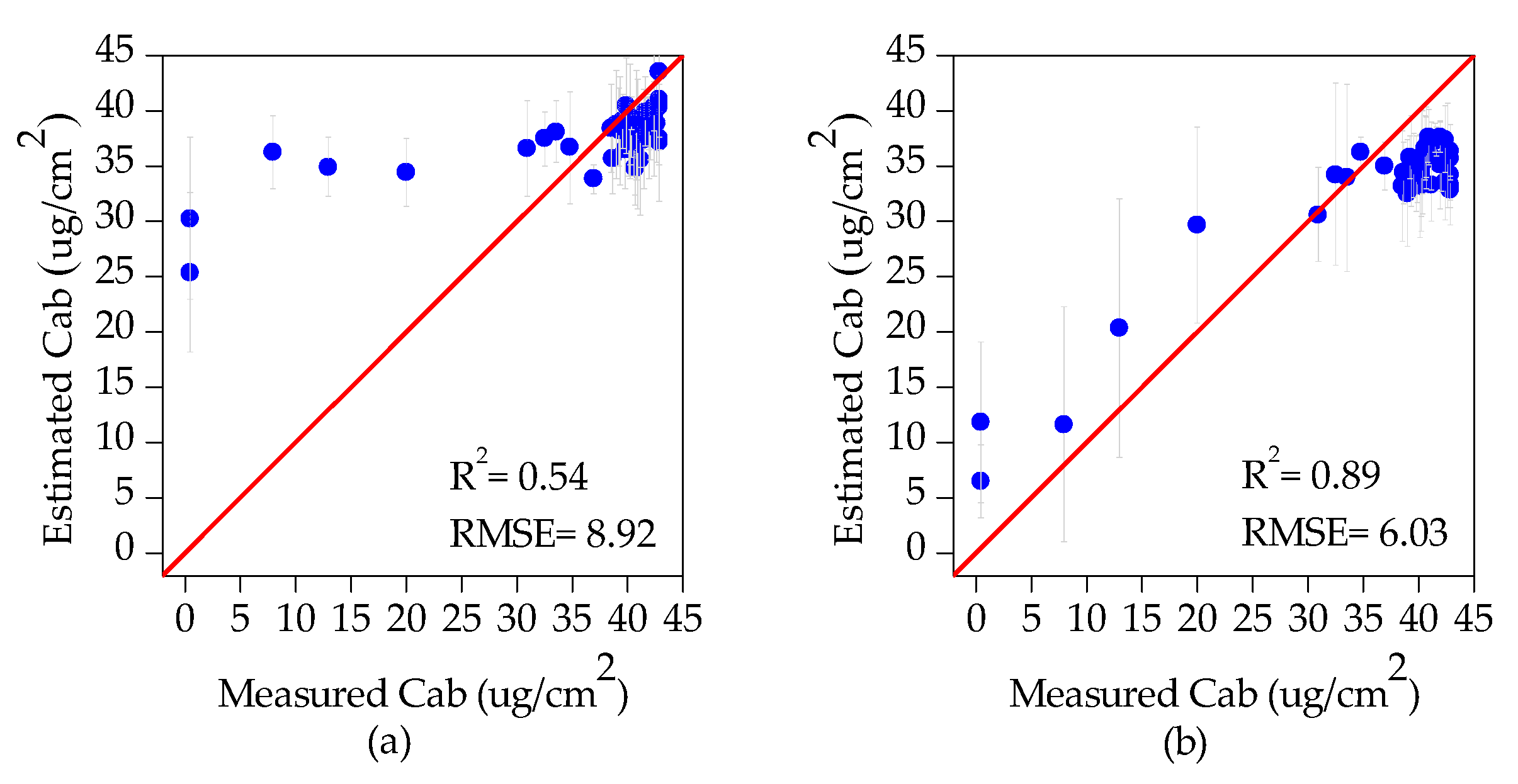
The underestimation of tree crown SDR was mainly caused by the overestimation of Cab (Figure 5a). During the tree crown delineation process using HI data, the damaged part of tree crown was severely underestimated, leading to the canopy reflectance change. This change caused the canopy reflectance characteristics of damaged trees to be similar (or close) to those of health tree crowns.
(3)
The exclusion of shaded pixels of tree crowns may cause the underestimation of tree damage severity by PSB insects because the shaded pixels may contain the damaged shoots.
In this study, lidar data were acquired on 4 September 2018, while the hyperspectral data were acquired on 21 September 2018. In the shoot-feeding time period, the shoot beetles should be more active. That means additional shoots may be attacked in this short time, resulting in more damaged trees than lidar data.

4.2. Contributions of Lidar

Lidar metrics were unable to effectively separate tree damage levels from slight to severe degrees (Figure 7). It is understandable that lidar data were difficult to accurately measure the biochemical characteristics of tree crowns [29,36,52]. However, it can be used as a supplementary information to provide accurate 3D tree crown structures (such as individual tree segmentation) [29]. Furthermore, the return intensity information can be used for estimating the reflection characteristics in the NIR region and spatial arrangement of different parts of the tree crown. More importantly, lidar data were useful for detecting dead trees (SDR > 80%) and their locations (Figure 10). Accurate detecting and mapping single dead trees is important to understand the spread direction and dynamics of the outbreak [80,81]. For example, a newly infested or dead tree may spread pests to neighbor trees leading to an infestation hot-spot in a short time. Due to climate change issues, the number of observed bark beetle generations are increasing [82]. Comprehensive utilization of high resolution remote sensing data may improve the ability to quickly estimate the scale of an outbreak in a large forest area, and consequently initiate appropriate activities to stop or at least limit its spread [80,83].
The intensity of lidar metrics calculated from first or all returns of tree crowns also played an additional contribution in estimating SDRs. Especially, the Int_Shd_top variable has the most importance in comparison to the other lidar metrics, if combined with hyperspectral variables. The lidar metric Int_Shd_top was determined by the shaded portions of tree crowns modeling. The voxel size and the threshold fdirect may also influence the accuracy of SDR estimation. A suitable voxel size (e.g., 0.3 m) could accurately depict the sunlit or shaded portions of shoots distribution within a crown. To test the best threshold, we defined a series of fdirect thresholds and calculated SDRs using RF (395 samples) with combined hyperspectral variable and lidar metrics. The results suggested that the fdirect threshold of 0.4 was the best performance for SDR estimation (Figure 11).

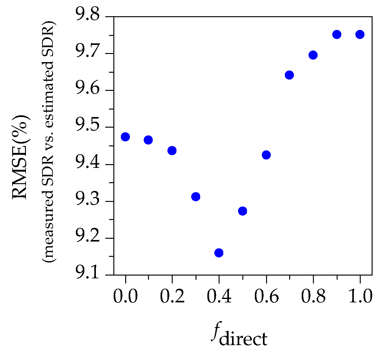
4.3. Possible Improvements of Inversion

According to the RF variable importance analysis, Cab and ACI are the two most important variables for the SDR estimation of individual tree crowns when hyperspectral data were combined with lidar metrics (Figure 9). Especially, Cab showed the highest sensitivity to tree crown stress, and thus contributed much more than other hyperspectral variables for measuring PSB damage. PROSAIL was regarded as a robust 1-D model to retrieve biochemical and biophysical parameters. However, PROSAIL still has limitations on simulating heterogeneous canopies (e.g., damaged canopy and shadow) [52]. Moreover, in the inversion of RTMs, the ill-posed problem always existed because the different combination of parameters have compensation effects on canopy reflectance, leading to very similar solutions if using the simplified assumptions of canopy model (e.g., 1-D model) [55,56]. These limitations and uncertainty problems may result in overestimation of Cab during the retrievals for damaged tree crowns (Figure 5). A promising way to improve Cab retrieval performance is to directly use 3D RTMs like RAPID to consider canopy heterogeneity with a given spatial arrangement of damaged shoots or leaves. This approach will be our next study.

4.4. SDR at Individual Tree Level

SDR was a useful indicator for detecting forest stand scale infection caused by shoot beetles [5]. This study provided a comprehensive knowledge of using an RF model to predict SDRs at individual tree level, at a more detailed scale. It provides a guidance on how to combine the advantages between hyperspectral and lidar data to assess single tree health using SDR indicators for forest management and conservation. Furthermore, this method can predict the damaged trees and their locations, as well as the special output of dead trees. It can then guide the forest managers to remove the potential outbreak sources at early stages to protect forest health.

5. Conclusions

In this study, we explored the potential of mapping tree crown damage severity by PSB insects using UAV-based HI and lidar measurements at individual tree level. We confirm that combing HI and lidar data reduced the SDR prediction errors from 15.87% or 12.28% to 9.93%. The proposed new shadow indicators contribute a lot to this improvement. This UAV-based approach provides critical information on tree crown damage severity at very small scales (e.g., crown scale), improving the possibility of PSB detection at early stage, and providing accurate single tree health measurement to prevent PSB insects spreading before the outbreak. In our next study, PROSAIL will be replaced by 3D RTMs to further improve the accuracy.

Author Contributions

Q.L. and H.H. conceived and designed the experiments; Q.L., J.W., K.H., and Y.L. conducted the field experiments; Q.L. analyzed the data; Q.L. wrote the paper.

Funding

This research was funded by National Natural Science Foundation of China: 41571332.

Acknowledgments

The authors would like to thank L. F. Yu and Huaguo Huang for the valuable advice on improving this paper.

Conflicts of Interest

The authors declare no conflict of interest.

References

  1. Waring, R.H.; Pitman, G.B. Modifying Lodgepole Pine Stands to Change Susceptibility to Mountain Pine Beetle Attack. Ecology 1985, 66, 889–897. [Google Scholar] [CrossRef]
  2. Ayres, M.P.; Lombardero, M.J. Assessing the consequences of global change for forest disturbance from herbivores and pathogens. Sci. Total Environ. 2000, 262, 263–286. [Google Scholar] [CrossRef]
  3. Wingfield, M.J.; Brockerhoff, E.G.; Wingfield, B.D.; Slippers, B. Planted forest health: The need for a global strategy. Science 2015, 349, 832–836. [Google Scholar] [CrossRef] [PubMed]
  4. Kautz, M.; Anthoni, P.; Meddens, A.J.H.; Pugh, T.A.M.; Arneth, A. Simulating the recent impacts of multiple biotic disturbances on forest carbon cycling across the United States. Glob. Chang. Biol. 2017, 24, 2079–2092. [Google Scholar] [CrossRef] [Green Version]
  5. Yu, L.; Huang, J.; Zong, S.; Huang, H.; Luo, Y. Detecting Shoot Beetle Damage on Yunnan Pine Using Landsat Time-Series Data. Forests 2018, 9, 39. [Google Scholar] [Green Version]
  6. Coulson, R.N.; Mcfadden, B.A.; Pulley, P.E.; Lovelady, C.N.; Fitzgerald, J.W.; Jack, S.B. Heterogeneity of forest landscapes and the distribution and abundance of the southern pine beetle. For. Ecol. Manag. 1999, 114, 471–485. [Google Scholar] [CrossRef]
  7. Townsend, P.A.; Singh, A.; Foster, J.R.; Rehberg, N.J.; Kingdon, C.C.; Eshleman, K.N.; Seagle, S.W. A general Landsat model to predict canopy defoliation in broadleaf deciduous forests. Remote Sens. Environ. 2012, 119, 255–265. [Google Scholar] [CrossRef]
  8. Foster, J.R.; Mladenoff, D.J. Spatial dynamics of a gypsy moth defoliation outbreak and dependence on habitat characteristics. Landsc. Ecol. 2013, 28, 1307–1320. [Google Scholar] [CrossRef]
  9. Senf, C.; Seidl, R.; Hostert, P. Remote sensing of forest insect disturbances: Current state and future directions. Int. J. Appl. Earth Obs. 2017, 60, 49–60. [Google Scholar] [CrossRef] [Green Version]
  10. Spruce, J.P.; Sader, S.; Ryan, R.E.; Smoot, J.; Kuper, P.; Ross, K.; Prados, D.; Russell, J.; Gasser, G.; McKellip, R.; et al. Assessment of MODIS NDVI time series data products for detecting forest defoliation by gypsy moth outbreaks. Remote Sens. Environ. 2011, 115, 427–437. [Google Scholar] [CrossRef]
  11. Somers, B.; Verbesselt, J.; Ampe, E.M.; Sims, N.; Verstraeten, W.W.; Coppin, P. Spectral mixture analysis to monitor defoliation in mixed-aged Eucalyptus globulus Labill plantations in southern Australia using Landsat 5-TM and EO-1 Hyperion data. Int. J. Appl. Earth Observ. Geoinf. 2010, 12, 270–277. [Google Scholar] [CrossRef]
  12. Kantola, T.; Vastaranta, M.; Yu, X.W.; Lyytikainensaarenmaa, P.; Holopainen, M.; Talvitie, M.; Kaasalainen, S.; Solberg, S.; Hyyppa, J. Classification of defoliated trees using tree-level airborne laser scanning data combined with aerial images. Remote Sens. Basel 2010, 2, 2665–2679. [Google Scholar] [CrossRef]
  13. Oumar, Z.M. Onisimo Integrating environmental variables and WorldView-2 image data to improve the prediction and mapping of Thaumastocoris peregrinus (bronze bug) damage in plantation forests. J. Photogramm. Remote Sens. 2014, 87, 39–46. [Google Scholar] [CrossRef]
  14. Meigs, G.W.; Kennedy, R.E.; Cohen, W.B. A Landsat time series approach to characterize bark beetle and defoliator impacts on tree mortality and surface fuels in conifer forests. Remote Sens. Environ. 2011, 115, 3707–3718. [Google Scholar] [CrossRef]
  15. Senf, C.; Pflugmacher, D.; Wulder, M.A.; Hostert, P. Characterizing spectral–temporal patterns of defoliator and bark beetle disturbances using Landsat time series. Remote Sens. Environ. 2015, 170, 166–177. [Google Scholar] [CrossRef]
  16. Amman, G.D. Mountain pine beetle—Identification, biology, causes of outbreaks, and entomological research needs. In BC-X-Canadian Forestry Service; Pacific Forest Research Centre: Victoria, BC, USA, 1982. [Google Scholar]
  17. Coops, N.C.; Johnson, M.; Wulder, M.A.; White, J.C. Assessment of QuickBird high spatial resolution imagery to detect red attack damage due to mountain pine beetle infestation. Remote Sens. Environ. 2006, 103, 67–80. [Google Scholar] [CrossRef]
  18. Wulder, M.A.; Dymond, C.C.; White, J.C.; Leckie, D.G.; Carroll, A.L. Surveying mountain pine beetle damage of forests: A review of remote sensing opportunities. For. Ecol. Manag. 2006, 221, 27–41. [Google Scholar] [CrossRef]
  19. Assal, T.J.; Sibold, J.; Reich, R. Modeling a Historical Mountain Pine Beetle Outbreak Using Landsat MSS and Multiple Lines of Evidence. Remote Sens. Environ. 2014, 155, 275–288. [Google Scholar] [CrossRef]
  20. Walter, J.A.; Platt, R.V. Multi-temporal analysis reveals that predictors of mountain pine beetle infestation change during outbreak cycles. For. Ecol. Manag. 2013, 302, 308–318. [Google Scholar] [CrossRef]
  21. West, D.R.; Briggs, J.S.; Jacobi, W.R.; Negrón, J.F. Mountain pine beetle-caused mortality over eight years in two pine hosts in mixed-conifer stands of the southern Rocky Mountains. For. Ecol. Manag. 2014, 334, 321–330. [Google Scholar] [CrossRef]
  22. Sprintsin, M.; Jing, M.C.; Czurylowicz, P. Combining land surface temperature and shortwave infrared reflectance for early detection of mountain pine beetle infestations in western Canada. J. Appl. Remote Sens. 2011, 5, 53566. [Google Scholar] [CrossRef]
  23. Coops, N.C.; Gillanders, S.N.; Wulder, M.A.; Gergel, S.E.; Nelson, T.; Goodwin, N.R. Assessing changes in forest fragmentation following infestation using time series Landsat imagery. For. Ecol. Manag. 2010, 259, 2355–2365. [Google Scholar] [CrossRef]
  24. Wulder, M.A.; White, J.C.; Coops, N.C.; Butson, C.R. Multi-temporal analysis of high spatial resolution imagery for disturbance monitoring. Remote Sens. Environ. 2008, 112, 2729–2740. [Google Scholar] [CrossRef]
  25. Wulder, M.A.; Ortlepp, S.M.; White, J.C.; Coops, N.C.; Coggins, S.B. Monitoring the impacts of mountain pine beetle mitigation. For. Ecol. Manag. 2009, 258, 1181–1187. [Google Scholar] [CrossRef]
  26. Lin, Q.; Huang, H.; Yu, L.; Wang, J. Detection of shoot beetle stress on yunnan pine forest using a coupled LIBERTY2-INFORM simulation. Remote Sens. Basel 2018, 10, 1133. [Google Scholar] [CrossRef]
  27. Meddens, A.J.H.; Hicke, J.A.; Vierling, L.A. Evaluating the potential of multispectral imagery to map multiple stages of tree mortality. Remote Sens. Environ. 2011, 115, 1632–1642. [Google Scholar] [CrossRef]
  28. Näsi, R.; Honkavaara, E.; Lyytikäinen-Saarenmaa, P.; Blomqvist, M.; Litkey, P.; Hakala, T.; Viljanen, N.; Kantola, T.; Tanhuanpää, T.; Holopainen, M. Using UAV-Based Photogrammetry and Hyperspectral Imaging for Mapping Bark Beetle Damage at Tree-Level. Remote Sens. Basel 2015, 7, 15467–15493. [Google Scholar] [CrossRef] [Green Version]
  29. Shendryk, I.; Broich, M.; Tulbure, M.G.; McGrath, A.; Keith, D.; Alexandrov, S.V. Mapping individual tree health using full-waveform airborne laser scans and imaging spectroscopy: A case study for a floodplain eucalypt forest. Remote Sens. Environ. 2016, 187, 202–217. [Google Scholar] [CrossRef]
  30. Cook, B.D.; Corp, L.A.; Nelson, R.F.; Middleton, E.M.; Morton, D.C.; Mccorkel, J.T.; Masek, J.G.; Ranson, K.J.; Ly, V.; Montesano, P.M. NASA goddard’s lidar, hyperspectral and thermal (G-LiHT) airborne imager. Remote Sens. Basel 2013, 5, 4045–4066. [Google Scholar] [CrossRef]
  31. Asner, G.P.; Martin, R.E.; Knapp, D.E.; Tupayachi, R.; Anderson, C.B.; Sinca, F.; Vaughn, N.R.; Llactayo, W. Airborne laser-guided imaging spectroscopy to map forest trait diversity and guide conservation. Science 2017, 355, 385. [Google Scholar] [CrossRef]
  32. Meng, R.; Dennison, P.E.; Zhao, F.; Shendryk, I.; Rickert, A.; Hanavan, R.P.; Cook, B.D.; Serbin, S.P. Mapping canopy defoliation by herbivorous insects at the individual tree level using bi-temporal airborne imaging spectroscopy and lidar measurements. Remote Sens. Environ. 2018, 215, 170–183. [Google Scholar] [CrossRef]
  33. Hanavan, R.P.; Jennifer, P.; Richard, H. A 10-Year Assessment of Hemlock Decline in the Catskill Mountain Region of New York State Using Hyperspectral Remote Sensing Techniques. J. Econ. Entomol. 2015, 108, 339–349. [Google Scholar] [CrossRef] [Green Version]
  34. Donoghue, D.N.M.; Watt, P.J.; Cox, N.J.; Wilson, J. Remote sensing of species mixtures in conifer plantations using lidar height and intensity data. Remote Sens. Environ. 2007, 110, 509–522. [Google Scholar] [CrossRef]
  35. Hovi, A.; Korhonen, L.; Vauhkonen, J.; Korpela, I. Lidar waveform features for tree species classification and their sensitivity to tree- and acquisition related parameters. Remote Sens. Environ. 2016, 173, 224–237. [Google Scholar] [CrossRef]
  36. Liu, L.; Coops, N.C.; Aven, N.W.; Pang, Y. Mapping urban tree species using integrated airborne hyperspectral and lidar remote sensing data. Remote Sens. Environ. 2017, 200, 170–182. [Google Scholar] [CrossRef]
  37. Höfle, B.; Pfeifer, N. Correction of laser scanning intensity data: Data and model-driven approaches. J. Photogramm. Remote Sens. 2007, 62, 415–433. [Google Scholar] [CrossRef]
  38. Solberg, S.; Næsset, E.; Hanssen, K.H.; Christiansen, E. Mapping defoliation during a severe insect attack on Scots pine using airborne laser scanning. Remote Sens. Environ. 2006, 102, 364–376. [Google Scholar] [CrossRef]
  39. Hanssen, H.K.; Solberg, S. Assessment of defoliation during a pine sawfly outbreak: Calibration of airborne laser scanning data with hemispherical photography. For. Ecol. Manag. 2007, 250, 9–16. [Google Scholar] [CrossRef]
  40. Senf, C.; Campbell, E.M.; Pflugmacher, D.; Wulder, M.A.; Hostert, P. A multi-scale analysis of western spruce budworm outbreak dynamics. Landsc. Ecol. 2017, 32, 501–514. [Google Scholar] [CrossRef]
  41. Ashton, E.A.; Wemett, B.D.; Leathers, R.A.; Downes, T.V. A novel method for illumination suppression in hyperspectral images. Proc. SPIE 2008, 6966, 69660C. [Google Scholar]
  42. Huang, H.; Qin, W.; Liu, Q. RAPID: A Radiosity Applicable to Porous IndiviDual Objects for directional reflectance over complex vegetated scenes. Remote Sens. Environ. 2013, 132, 221–237. [Google Scholar] [CrossRef]
  43. Yuan, J.; Wang, D.L.; Li, R. Remote Sensing Image Segmentation by Combining Spectral and Texture Features. IEEE Trans. Geosci. Remote Sens. 2014, 52, 16–24. [Google Scholar] [CrossRef]
  44. Sauvola, J.; Pietikäinen, M. Adaptive document image binarization. Pattern Recogn. 2000, 33, 225–236. [Google Scholar] [CrossRef] [Green Version]
  45. Zarco-Tejadaa, P.J.; Hornerob, A.; Becka, P.S.A.; Kattenbornd, T.; Kempeneersa, P. Chlorophyll content estimation in an open-canopy conifer forest with Sentinel-2A and hyperspectral imagery in the context of forest decline. Remote Sens. Environ. 2019, 223, 320–335. [Google Scholar] [CrossRef]
  46. Zhao, X.; Guo, Q.; Su, Y.; Xue, B. Improved progressive TIN densification filtering algorithm for airborne lidar data in forested areas. J. Photogramm. Remote Sens. 2016, 117, 79–91. [Google Scholar] [CrossRef]
  47. Li, W.; Guo, Q.; Jakubowski, M.K.; Kelly, M. A new method for segmenting individual trees from the lidar point cloud. Photogramm. Eng. Remote Sens. 2012, 78, 75–84. [Google Scholar] [CrossRef]
  48. Janoutová, R.; Homolová, L.; Malenovský, Z.; Hanuš, J.; Lauret, N.; Gastellu-Etchegorry, J. Influence of 3D Spruce Tree Representation on Accuracy of Airborne and Satellite Forest Reflectance Simulated in DART. Forests 2019, 10, 292. [Google Scholar] [CrossRef]
  49. MacArthur, R.H.; Horn, H.S. Foliage profile by vertical measurements. Ecology 1969, 50, 802–804. [Google Scholar] [CrossRef]
  50. Almeida, D.R.A.D.; Stark, S.C.; Shao, G.; Schietti, J.; Nelson, B.W.; Silva, C.A.; Gorgens, E.B.; Valbuena, R.; Papa, D.D.A.; Brancalion, P.H.S. Optimizing the Remote Detection of Tropical Rainforest Structure with Airborne lidar: Leaf Area Profile Sensitivity to Pulse Density and Spatial Sampling. Remote Sens. Basel 2019, 11, 92. [Google Scholar] [CrossRef]
  51. Martin, R.; Chadwick, K.; Brodrick, P.; Carranza-Jimenez, L.; Vaughn, N.; Asner, G. An Approach for Foliar Trait Retrieval from Airborne Imaging Spectroscopy of Tropical Forests. Remote Sens. Basel 2018, 10, 199. [Google Scholar] [CrossRef]
  52. Shi, Y.; Skidmore, A.K.; Wang, T.; Holzwarth, S.; Heiden, U.; Pinnel, N.; Zhu, X.; Heurich, M. Tree species classification using plant functional traits from lidar and hyperspectral data. Int. J. Appl. Earth Obs. 2018, 73, 207–219. [Google Scholar] [CrossRef]
  53. Shi, Y.; Wang, T.; Skidmore, A.K.; Heurich, M. Important lidar metrics for discriminating forest tree species in Central Europe. ISPRS J. Photogramm. Remote Sens. 2018, 137, 163–174. [Google Scholar] [CrossRef]
  54. Lin, Y.; Hyyppä, J. A comprehensive but efficient framework of proposing and validating feature parameters from airborne lidar data for tree species classification. Int. J. Appl. Earth Obs. 2016, 46, 45–55. [Google Scholar] [CrossRef]
  55. Rivera, J.; Verrelst, J.; Leonenko, G.; Moreno, J. Multiple Cost Functions and Regularization Options for Improved Retrieval of Leaf Chlorophyll Content and LAI through Inversion of the PROSAIL Model. Remote Sens. Basel 2013, 5, 3280–3304. [Google Scholar] [CrossRef] [Green Version]
  56. Verrelst, J.; Rivera, J.P.; Leonenko, G.; Alonso, L.; Moreno, J. Optimizing LUT-Based RTM Inversion for Semiautomatic Mapping of Crop Biophysical Parameters from Sentinel-2 and -3 Data: Role of Cost Functions. IEEE T Geosci. Remote 2014, 52, 257–269. [Google Scholar] [CrossRef]
  57. Ferreira, M.P.; Féret, J.; Grau, E.; Gastellu-Etchegorry, J.; Do Amaral, C.H.; Shimabukuro, Y.E.; de Souza Filho, C.R. Retrieving structural and chemical properties of individual tree crowns in a highly diverse tropical forest with 3D radiative transfer modeling and imaging spectroscopy. Remote Sens. Environ. 2018, 211, 276–291. [Google Scholar] [CrossRef]
  58. Jacquemoud, S.; Verhoef, W.; Baret, F.; Bacour, C.; Zarco-Tejada, P.J.; Asner, G.P.; François, C.; Ustin, S.L. PROSPECT+SAIL models: A review of use for vegetation characterization. Remote Sens. Environ. 2009, 113, S56–S66. [Google Scholar] [CrossRef]
  59. Jacquemoud, S.; Baret, F. PROSPECT: A model of leaf optical properties spectra. Remote Sens. Environ. 1990, 34, 75–91. [Google Scholar] [CrossRef]
  60. Verhoef, W.; Jia, L.; Xiao, Q.; Su, Z. Unified Optical-Thermal Four-Stream Radiative Transfer Theory for Homogeneous Vegetation Canopies. IEEE Trans. Geosci. Remote 2007, 45, 1808–1822. [Google Scholar] [CrossRef]
  61. Féret, J.B.; Gitelson, A.A.; Noble, S.D.; Jacquemoud, S. PROSPECT-D: Towards modeling leaf optical properties through a complete lifecycle. Remote Sens. Environ. 2017, 193, 204–215. [Google Scholar] [CrossRef] [Green Version]
  62. Ali, A.M.; Skidmore, A.K.; Darvishzadeh, R.; Duren, I.V.; Holzwarth, S.; Mueller, J. Retrieval of forest leaf functional traits from HySpex imagery using radiative transfer models and continuous wavelet analysis. ISPRS J. Photogramm. Remote Sens. 2016, 122, 68–80. [Google Scholar] [CrossRef] [Green Version]
  63. Breiman, L. Random Forests. Mach. Learn. 2001, 45, 5–32. [Google Scholar] [CrossRef] [Green Version]
  64. Mutanga, O.; Adam, E.; Cho, M.A. High density biomass estimation for wetland vegetation using WorldView-2 imagery and random forest regression algorithm. Int. J. Appl. Earth Obs. 2012, 18, 399–406. [Google Scholar] [CrossRef]
  65. Archer, K.J.; Kimes, R.V. Empirical characterization of random forest variable importance measures. Comput. Stat. Data Ann. 2008, 52, 2249–2260. [Google Scholar] [CrossRef]
  66. Verikas, A.; Gelzinis, A.; Bacauskiene, M. Mining data with random forests: A survey and results of new tests. Pattern Recogn. 2011, 44, 330–349. [Google Scholar] [CrossRef]
  67. Abdel-Rahman, E.M.; Ahmed, F.B.; Ismail, R. Random forest regression and spectral band selection for estimating sugarcane leaf nitrogen concentration using EO-1 Hyperion hyperspectral data. Int. J. Remote Sens. 2013, 34, 712–728. [Google Scholar] [CrossRef]
  68. Immitzer, M.; Atzberger, C.; Koukal, T. Tree Species Classification with Random Forest Using Very High Spatial Resolution 8-Band WorldView-2 Satellite Data. Remote Sens. Basel 2012, 4, 2661–2693. [Google Scholar] [CrossRef] [Green Version]
  69. Liaw, A.; Wiener, M. Classification and Regression by RandomForest. R. News 2002, 2, 18–22. [Google Scholar]
  70. Chen, J.M. Evaluation of Vegetation Indices and a Modified Simple Ratio for Boreal Applications. Can. J. Remote Sens. 1996, 22, 229–242. [Google Scholar] [CrossRef]
  71. Sims, D.A.; Gamon, J.A. Relationships between leaf pigment content and spectral reflectance across a wide range of species, leaf structures and developmental stages. Remote Sens. Environ. 2002, 81, 337–354. [Google Scholar] [CrossRef]
  72. Rouse, J.W., Jr.; Haas, R.H.; Schell, J.A.; Deering, D.W. Monitoring Vegetation Systems in the Great Plains with ERTS. NASA Spec. Publ. 1974, 1, 309–317. [Google Scholar]
  73. Gamon, J.A.; Surfus, J.S. Assessing Leaf Pigment Content and Activity with a Reflectometer. N. Phytol. 2010, 143, 105–117. [Google Scholar] [CrossRef]
  74. Carter, G.A.; Miller, R.L. Early detection of plant stress by digital imaging within narrow stress-sensitive wavebands. Remote Sens. Environ. 1994, 50, 295–302. [Google Scholar] [CrossRef]
  75. Blackburn, G.A. Quantifying Chlorophylls and Caroteniods at Leaf and Canopy Scales: An Evaluation of Some Hyperspectral Approaches. Remote Sens. Environ. 1998, 66, 273–285. [Google Scholar] [CrossRef]
  76. Babar, M.A.; Reynolds, M.P.; van Ginkel, M.; Klatt, A.R.; Raun, W.R.; Stone, M.L. Spectral Reflectance Indices as a Potential Indirect Selection Criteria for Wheat Yield under Irrigation. Crop. Sci. 2006, 46, 578. [Google Scholar] [CrossRef]
  77. Pontius, J.; Martin, M.; Plourde, L.; Hallett, R. Ash decline assessment in emerald ash borer-infested regions: A test of tree-level, hyperspectral technologies. Remote Sens. Environ. 2008, 112, 2665–2676. [Google Scholar] [CrossRef]
  78. Ma, Y.; Min, H.; Bao, Y.; Zhu, Q. Automatic threshold method and optimal wavelength selection for insect-damaged vegetable soybean detection using hyperspectral images. Compute. Electr. Agricult. 2014, 106, 102–110. [Google Scholar] [CrossRef]
  79. Tochon, G.; Féret, J.B.; Valero, S.; Martin, R.E.; Knapp, D.E.; Salembier, P.; Chanussot, J.; Asner, G.P. On the use of binary partition trees for the tree crown segmentation of tropical rainforest hyperspectral images. Remote Sens. Environ. 2015, 159, 318–331. [Google Scholar] [CrossRef] [Green Version]
  80. Stereńczak, K.; Mielcarek, M.; Modzelewska, A.; Kraszewski, B.; Fassnacht, F.E.; Hilszczański, J. Intra-annual Ips typographus outbreak monitoring using a multi-temporal GIS analysis based on hyperspectral and ALS data in the Białowieża Forests. For. Ecol. Manag. 2019, 442, 105–116. [Google Scholar] [CrossRef]
  81. Wermelinger, B. Ecology and management of the spruce bark beetle Ips typographus—A review of recent research. For. Ecol. Manag. 2004, 202, 67–82. [Google Scholar] [CrossRef]
  82. Jonsson, A.M.; Appelberg, G.; Harding, S.; Barring, L. Spatio-temporal impact of climate change on the activity and voltinism of the spruce bark beetle. IPS. Typogr. 2009, 15, 486–499. [Google Scholar] [CrossRef]
  83. Kautz, M.; Kai, D.; Gruppe, A.; Schopf, R. Quantifying spatio-temporal dispersion of bark beetle infestations in epidemic and non-epidemic conditions. For. Ecol. Manag. 2011, 262, 598–608. [Google Scholar] [CrossRef]
Figure 1. The location of the study sites and unmanned airborne vehicles (UAV) flight areas. The red rectangle represents two field plots locations, and the purple and yellow rectangles represent hyperspectral and lidar flight areas, respectively.
Remotesensing 11 02540 g001
Figure 2. Image segmentation results: (a) the original hyperspectral imaging (HI) (false color composition); (b) the segmentation of the crowns, soil and shadows; and (c) the segmented sunlit crowns.
Remotesensing 11 02540 g002
Figure 3. (a) HI data; (b) 3D forest scene with sunlit and shaded tree crowns modelling by RAPID (top-view); (c) classifying cloud points into sunlit and shaded portions (side-view).
Remotesensing 11 02540 g003
Figure 4. The different spatial arrangement of tree crowns; (a) the vertical height; and (b) the horizontal direction.
Remotesensing 11 02540 g004
Figure 5. Measured vs. estimated Cab (215 samples) using different tree crown delineations: (a) from only hyperspectral segmentation; and (b) from only lidar segmentation.
Remotesensing 11 02540 g005
Figure 6. The mean reflectance value of different SDR at 400–1000 nm wavelengths.
Remotesensing 11 02540 g006
Figure 7. Comparison of different SDR ranges of ten variables derived from hyperspectral variables and lidar metrics.
Remotesensing 11 02540 g007
Figure 8. Measured vs. estimated SDR (215 samples) using three different approaches: (a) lidar approach, (b) hyperspectral approach, and (c) combined approach; each point represents the mean (and associated ± 1SD bar) of SDR parameter that yielded the five nearest measured values of the individual tree crown.
Remotesensing 11 02540 g008
Figure 9. The mean decrease accuracy (MDA) of each variable for SDR estimation, with a combination of hyperspectral variables and lidar metrics.
Remotesensing 11 02540 g009
Figure 10. (a) Dead trees and their locations mapping using the lidar approach in the lidar flight area; (b) tree crown SDR mapping using the combined approach in the hyperspectral flight area.
Remotesensing 11 02540 g010
Figure 11. The impact of threshold fdirect on the RMSE of SDR estimation.
Remotesensing 11 02540 g011
Table 1. Statistics of two plots variables (tree numbers = 448). H: Tree height; CBH: Crown base height; DBH: Diameter at breast height; CD: Crown diameter; Cab: Leaf chlorophyll content; SDR: Shoot damage ratio.
MeanStandard DeviationMaximum Minimum Range
H (m)4.51.69.81.28.6
CBH (cm)2.51.25.80.55.3
DBH (cm)8.94.0252.522.5
CD (m)2.21.07.30.56.8
Cab (mg/cm2)32.314.942.80.542.3
SDR (%)26351000100
Table 2. Input parameters and ranges of PROSAIL used for generating the LUT.
ParametersUnitRange
NStructure parameter-1.5–2.5
CmLeaf mass per areag cm−20.005–0.035
CabLeaf chlorophyll contentμg cm−20.5–43
CwEquivalent water thicknesscm0.01
CarCarotenoid contentμg cm−23–12
CanthAnthocyanin content μg cm−20.1–4
LAILeaf area index-0.25–3.5
ALAAverage leaf angledegree30–70
hspotHot spot size-0.01
ttsSolar zenith angledegree25
ttoObserver zenith angledegree0
psiRelative azimuth angledegree0
Table 3. Features selection of hyperspectral variables.
VariablesIndex or DescriptionFormulaReference
MSRModified simple ratioMSR = ((R800/R670) − 1) / sqrt ((R800/R670) + 1)[70]
SR _680Narrowband simple ratio 680SR _680 = R800 / R680[71]
SR _705Narrowband simple ratio 705SR _705 = R750 / R705[71]
NDVINormalized Difference Vegetation IndexNDVI = (R800− R670)/(R800+ R670)[72]
ACIAnthocyanin content index A C I = i = 600 i = 700 R i / i = 500 i = 600 R i [73]
PSIPlant stress indexPSI = R695/R760[74]
RVSI1Ratio vegetation stress indexRVSI1 = R600/ R760[74]
RVSI2Ratio vegetation stress indexRVSI2 = R710/ R760[74]
PSSRPigment specific simple ratioPSSR = R800/ R635[75]
NWINormalized water indexNWI = (R970 − R850) / (R970+R850)[76]
CabLeaf chlorophyll content
where Ri is the reflectance at the i wavelength, and sqrt is square root.
Table 4. Features selection of lidar metrics.
VariablesDefinition
Int_mean_firstMean value of crown first return intensity
Int_CVCoefficient of variation of crown return intensity
Int_P2525th percentile of crown return intensity
Int_P7575th percentile of crown return intensity
Int_C2525h cumulative percentile of crown return intensity
Int_C5050h cumulative percentile of crown return intensity
Int_CV_SE_TopCoefficient of variation of the top of SE crown return intensity
Int_mean_NW_TopMean value of the top of NW crown return intensity
Int_mean_NE&SW_TopMean value of the top of NE and SW crown return intensity
Int_CV_first_E_TopCoefficient of variation of the top of E crown first return intensity
Int_mean_N&SE_TopMean value of the top of N and SE crown return intensity
Int_Shd_TopMean value of the top of shaded crown return intensity
CDCrown density
GFGap fraction
Table 5. Comparison of the lidar and combined approach on the classification accuracy of different damaged degrees.
Healthy SlightlyModeratelySeverelyDead
SDR: 0–10%SDR: 10–30%SDR: 30–50%SDR: 50–80%SDR: 80–100%
Combined approach7069162988
Lidar approach4166 82170
Note: a total of 395 samples from lidar segmentation were used for accuracy assessment.

