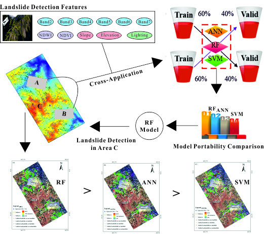
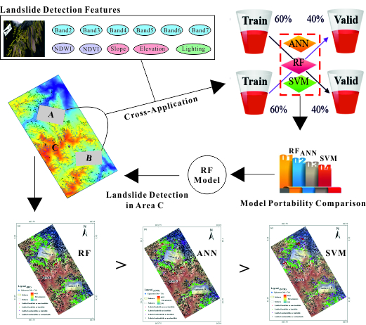
Improving the Accuracy of Landslide Detection in “Off-site” Area by Machine Learning Model Portability Comparison: A Case Study of Jiuzhaigou Earthquake, China

Abstract
:
1. Introduction
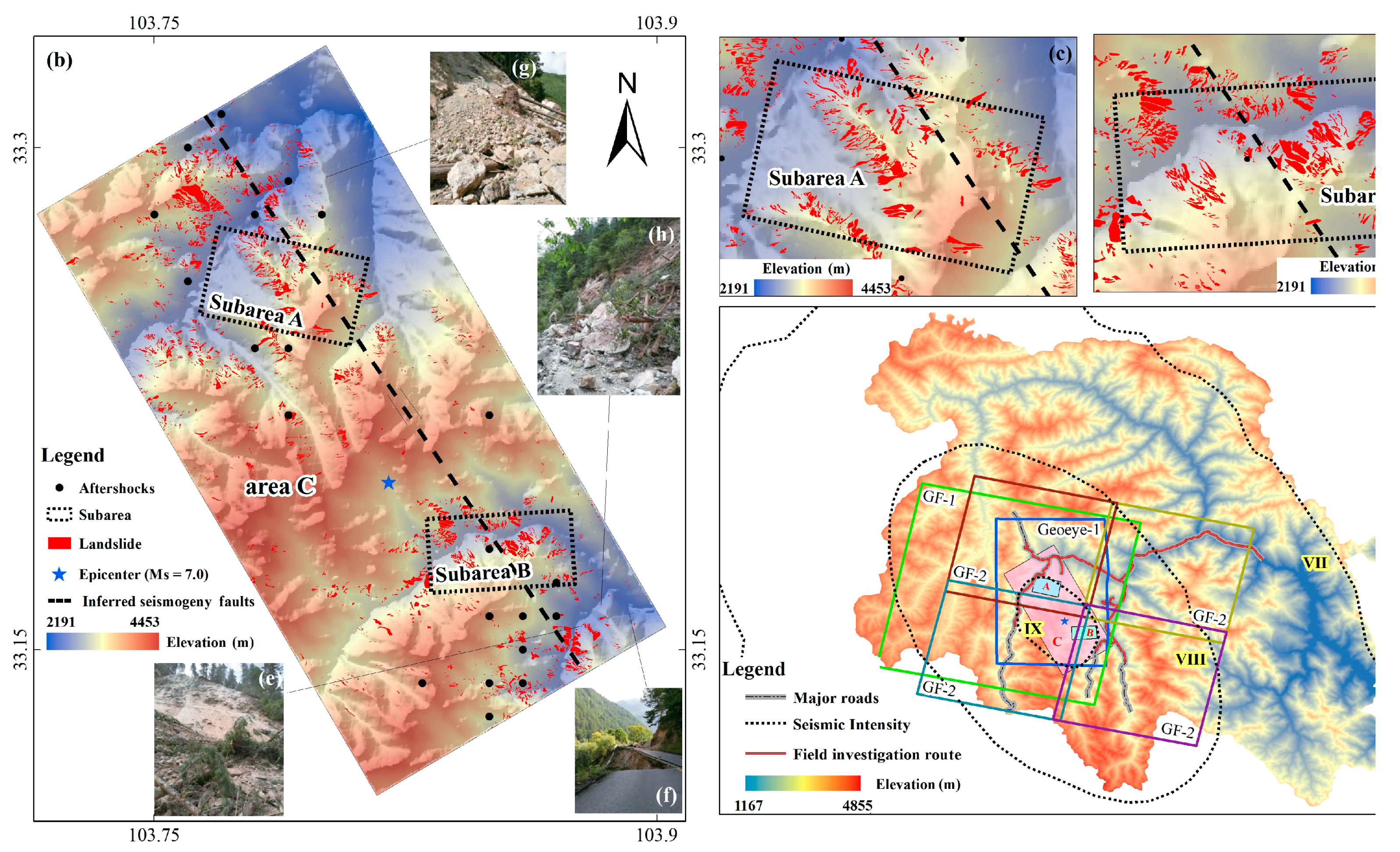
2. Study Area
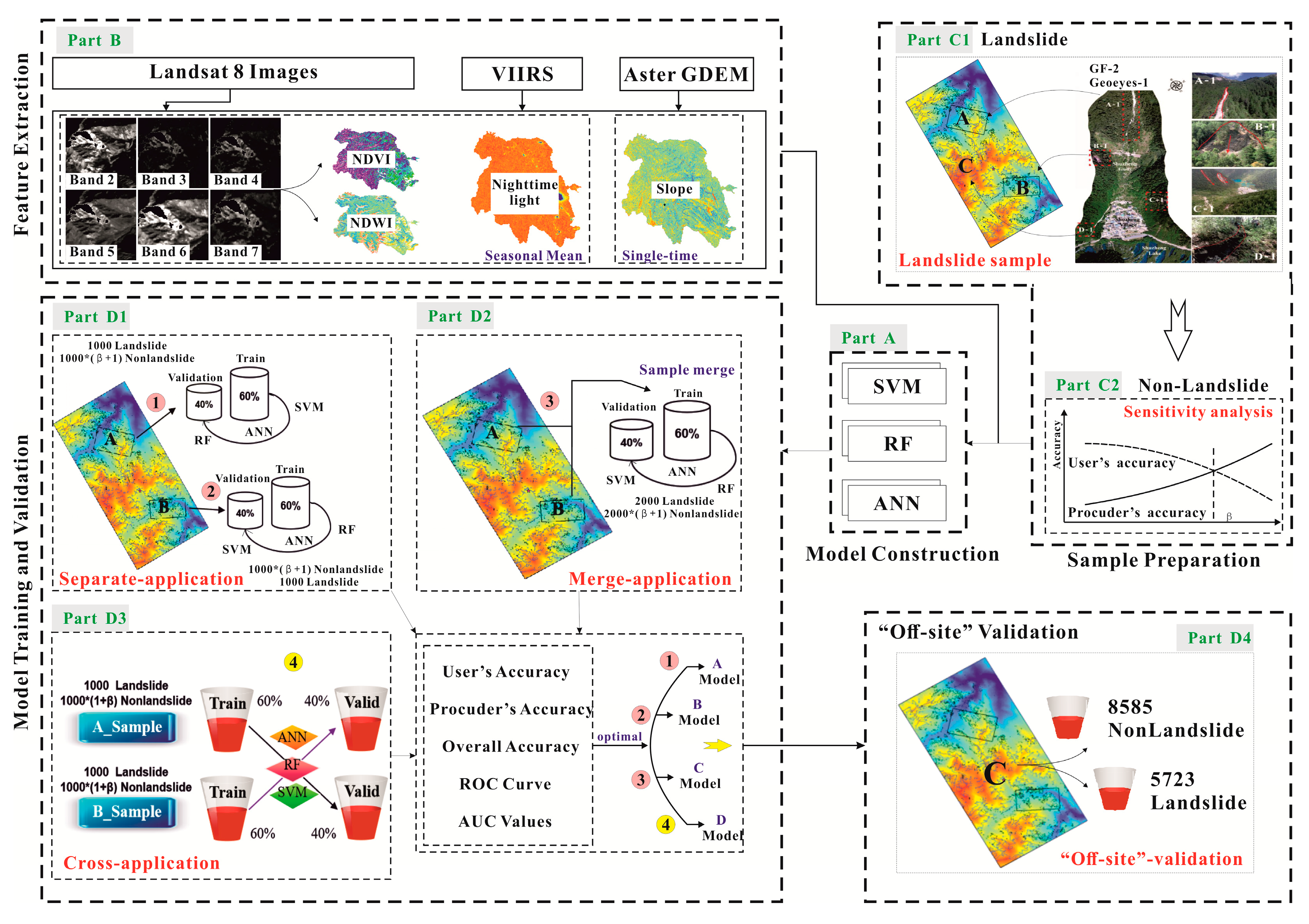
3. Materials and Methods
3.1. Applied ML Model
3.1.1. SVM Model
3.1.2. ANN Model
3.1.3. RF Model
3.2. Data Used
3.2.1. Image Features for Landslide Detection
3.2.2. Landslide Inventory
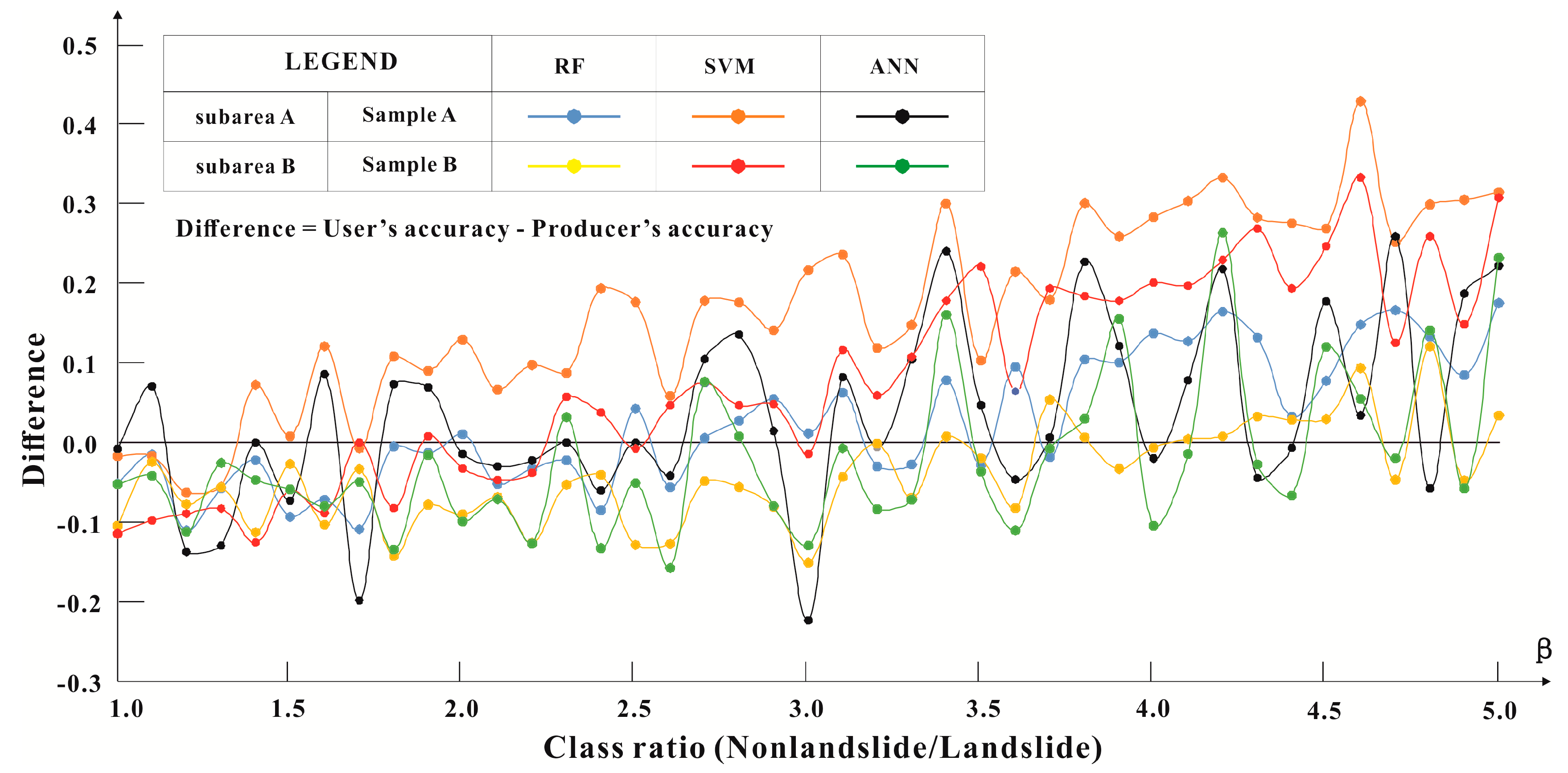
3.3. Sensitivity Analysis
4. Results
4.1. Separated-Application
4.2. Merged-Application
4.3. Cross-Application
4.3.1. Portability of the Three Models to Subarea B
4.3.2. Portability of the Three Models to Subarea A
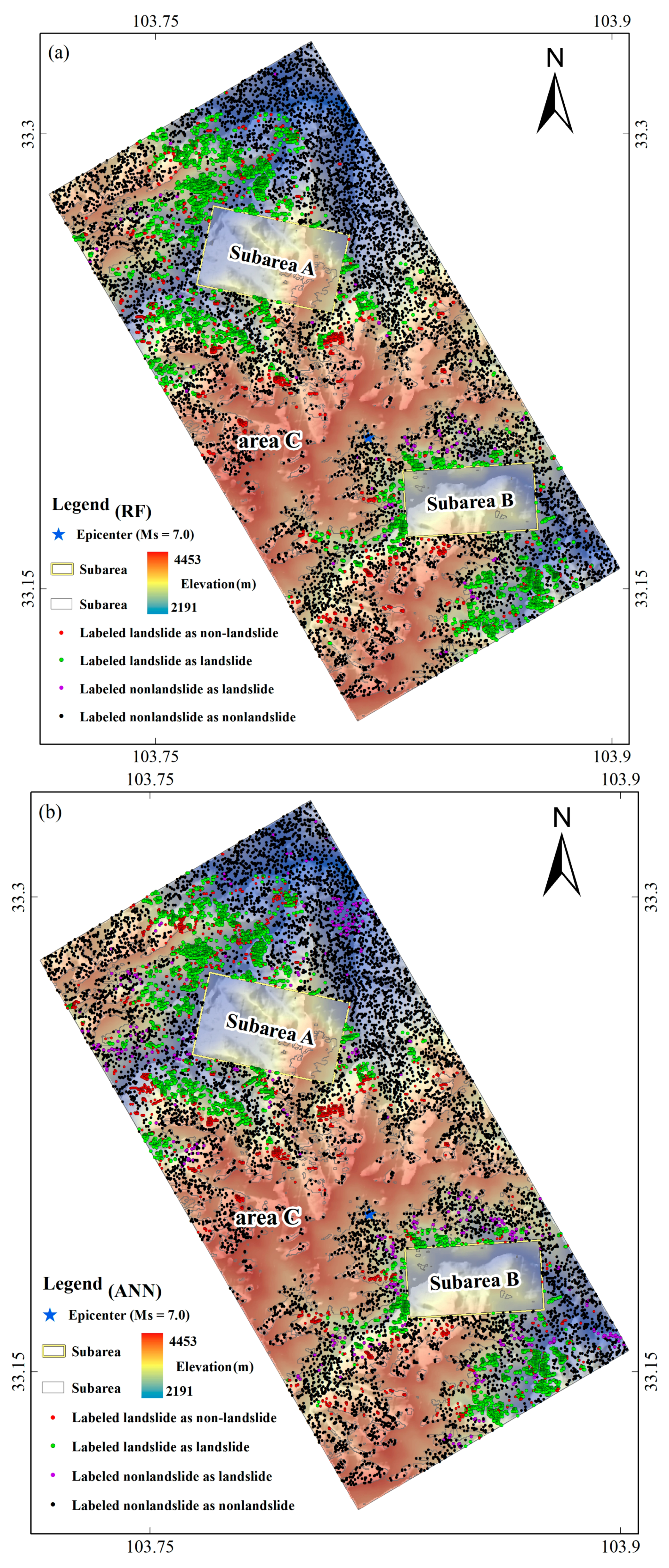
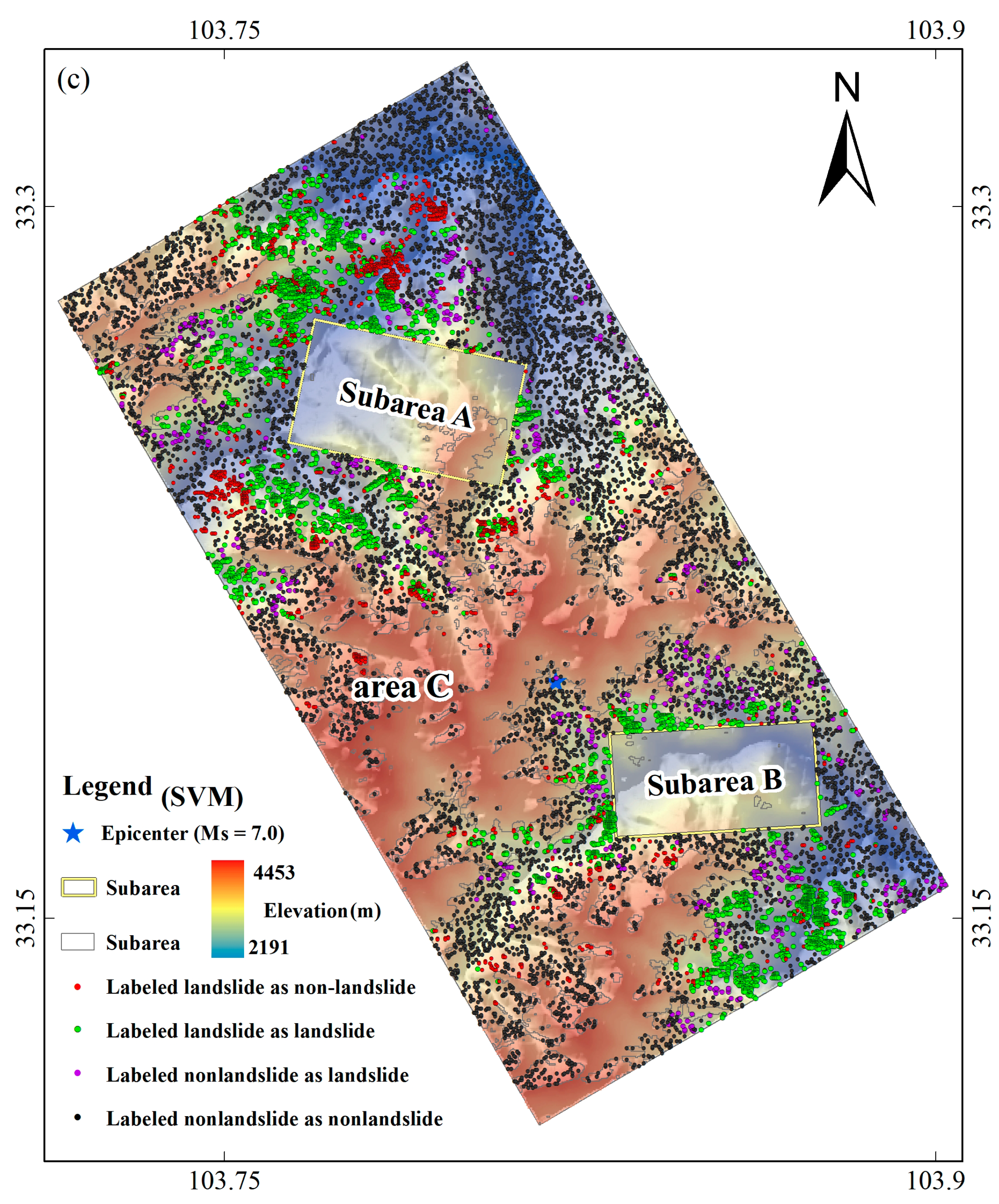
4.4. “Off-site” Area Application and Validation
5. Discussions
6. Conclusions
Author Contributions
Funding
Acknowledgments
Conflicts of Interest
Appendix A

| β | Subarea A | Subarea B | Standard Deviation | Distance Index | ||||
|---|---|---|---|---|---|---|---|---|
| RF | SVM | ANN | RF | SVM | ANN | |||
| 1.2 | −0.11 | −0.06 | −0.14 | −0.08 | −0.09 | −0.11 | 0.027 | 0.248 |
| 1.3 | −0.06 | −0.06 | −0.13 | −0.06 | −0.08 | −0.03 | 0.035 | 0.184 |
| 1.5 | −0.09 | 0.01 | −0.07 | −0.03 | −0.06 | −0.06 | 0.036 | 0.147 |
| 1 | −0.05 | −0.02 | −0.01 | −0.10 | −0.11 | −0.05 | 0.044 | 0.172 |
| 2.1 | −0.05 | 0.07 | −0.03 | −0.07 | −0.05 | −0.07 | 0.051 | 0.141 |
| 2.3 | −0.02 | 0.09 | 0.00 | −0.05 | 0.06 | 0.03 | 0.052 | 0.123 |
| 1.1 | −0.02 | −0.02 | 0.07 | −0.02 | −0.10 | −0.04 | 0.054 | 0.131 |
| 1.9 | −0.01 | 0.09 | 0.07 | −0.08 | 0.01 | −0.02 | 0.061 | 0.139 |
| 3.2 | −0.03 | 0.12 | −0.01 | 0.00 | 0.06 | −0.08 | 0.071 | 0.160 |
| 1.4 | −0.02 | 0.07 | 0.00 | −0.11 | −0.13 | −0.05 | 0.074 | 0.191 |
| 1.7 | −0.11 | −0.01 | −0.20 | −0.03 | 0.00 | −0.05 | 0.075 | 0.234 |
| 2.7 | 0.01 | 0.18 | 0.10 | −0.05 | 0.08 | 0.08 | 0.079 | 0.237 |
| 2.2 | −0.03 | 0.10 | −0.02 | −0.13 | −0.04 | −0.13 | 0.082 | 0.210 |
| 2 | 0.01 | 0.13 | −0.01 | −0.09 | −0.03 | −0.10 | 0.083 | 0.190 |
| 2.8 | 0.03 | 0.18 | 0.14 | −0.06 | 0.05 | 0.01 | 0.085 | 0.235 |
| 2.9 | 0.05 | 0.14 | 0.01 | −0.08 | 0.05 | −0.08 | 0.085 | 0.195 |
| 2.6 | −0.06 | 0.06 | −0.04 | −0.13 | 0.05 | −0.16 | 0.088 | 0.226 |
| 4.5 | 0.08 | 0.27 | 0.18 | 0.03 | 0.25 | 0.12 | 0.095 | 0.430 |
| 3.7 | −0.02 | 0.18 | 0.01 | 0.05 | 0.19 | −0.01 | 0.095 | 0.270 |
| 3.9 | 0.10 | 0.26 | 0.12 | −0.03 | 0.18 | 0.15 | 0.097 | 0.385 |
| 3.1 | 0.06 | 0.24 | 0.08 | −0.04 | 0.12 | −0.01 | 0.098 | 0.285 |
| 1.6 | −0.07 | 0.12 | 0.09 | −0.10 | −0.09 | −0.08 | 0.099 | 0.227 |
| 3.3 | −0.03 | 0.15 | 0.10 | −0.07 | 0.11 | −0.07 | 0.099 | 0.234 |
| 3.5 | −0.03 | 0.10 | 0.05 | −0.02 | 0.22 | −0.04 | 0.100 | 0.253 |
| 2.5 | 0.04 | 0.18 | 0.00 | −0.13 | −0.01 | −0.05 | 0.102 | 0.228 |
| 5 | 0.17 | 0.31 | 0.22 | 0.03 | 0.31 | 0.23 | 0.103 | 0.572 |
| 3.4 | 0.08 | 0.30 | 0.24 | 0.01 | 0.18 | 0.16 | 0.106 | 0.459 |
| 1.8 | 0.00 | 0.11 | 0.07 | −0.14 | −0.08 | −0.13 | 0.106 | 0.249 |
| 4.2 | 0.16 | 0.33 | 0.22 | 0.01 | 0.23 | 0.26 | 0.110 | 0.553 |
| 3.8 | 0.10 | 0.30 | 0.23 | 0.01 | 0.18 | 0.03 | 0.115 | 0.432 |
| 2.4 | −0.08 | 0.19 | −0.06 | −0.04 | 0.04 | −0.13 | 0.116 | 0.262 |
| 4.1 | 0.13 | 0.30 | 0.08 | 0.00 | 0.20 | −0.01 | 0.120 | 0.391 |
| 3.6 | 0.09 | 0.21 | −0.05 | −0.08 | 0.06 | −0.11 | 0.124 | 0.283 |
| 4.8 | 0.13 | 0.30 | −0.06 | 0.12 | 0.26 | 0.14 | 0.125 | 0.459 |
| 4.4 | 0.03 | 0.27 | −0.01 | 0.03 | 0.19 | −0.07 | 0.130 | 0.345 |
| 4.7 | 0.17 | 0.25 | 0.26 | −0.05 | 0.13 | −0.02 | 0.131 | 0.419 |
| 4.9 | 0.08 | 0.30 | 0.19 | −0.05 | 0.15 | −0.06 | 0.140 | 0.403 |
| 4.3 | 0.13 | 0.28 | −0.04 | 0.03 | 0.27 | −0.03 | 0.144 | 0.415 |
| 4 | 0.14 | 0.28 | −0.02 | −0.01 | 0.20 | −0.10 | 0.148 | 0.387 |
| 3 | 0.01 | 0.22 | −0.22 | −0.15 | −0.01 | −0.13 | 0.156 | 0.369 |
| 4.6 | 0.15 | 0.43 | 0.03 | 0.09 | 0.33 | 0.05 | 0.161 | 0.573 |
| Landslide_Related Features | Weight Calculated by RF Model |
|---|---|
| summer_ndvi | 0.29301622 |
| autumn_ndvi | 0.10382754 |
| elevation | 0.10074204 |
| summer_band 4 | 0.06635309 |
| summer_band 7 | 0.06287415 |
| winter_ndvi | 0.04509334 |
| slope | 0.03764887 |
| summer_band 2 | 0.03555093 |
| summer_ndwi | 0.02913229 |
| summer_band 5 | 0.02501019 |
| winter_band 2 | 0.02171738 |
| autumn_ndwi | 0.01790977 |
| spring_nighttime light | 0.01509238 |
| summer_nighttime light | 0.01455534 |
| winter_nighttime light | 0.01375868 |
| autumn_nighttime light | 0.01205927 |
| winter_band 4 | 0.01161285 |
| summer_band 3 | 0.0115633 |
| winter_ndwi | 0.00959292 |
| winter_band 3 | 0.00868868 |
| summer_band 6 | 0.00812666 |
| winter_band 5 | 0.00747098 |
| autumn_band 2 | 0.00738832 |
| autumn_band 3 | 0.00720624 |
| autumn_band 5 | 0.00719601 |
| autumn_band 7 | 0.00568052 |
| winter_band 7 | 0.00559739 |
| autumn_band 4 | 0.00524157 |
| autumn_band 6 | 0.00519584 |
| winter_band 6 | 0.00509723 |
References
- Guzzetti, F.; Mondini, A.C.; Cardinali, M.; Fiorucci, F.; Santangelo, M.; Chang, K.T. Landslide inventory maps: New tools for an old problem. Earth. Sci. Rev. 2012, 112, 42–66. [Google Scholar] [CrossRef] [Green Version]
- Pradhan, A.M.S.; Tarolli, P.; Kang, H.S.; Lee, J.S.; Kim, Y.T. Shallow landslide susceptibility modeling incorporating rainfall statistics: A case study from the Deokjeok-ri Watershed, South Korea. Int. J. Erosion. Control. Eng. 2016, 9, 18–24. [Google Scholar] [CrossRef]
- Guzzetti, F.; Cardinali, M.; Reichenbach, P.; Cipolla, F.; Sebastiani, C.; Galli, M.; Salvati, P. Landslides triggered by the 23 November 2000 rainfall event in the Imperia Province, Western Liguria, Italy. Eng. Geol. 2004, 73, 229–245. [Google Scholar] [CrossRef]
- Mondini, A.C.; Guzzetti, F.; Reichenbach, P.; Rossi, M.; Cardinali, M.; Ardizzone, F. Semi-automatic recognition and mapping of rainfall induced shallow landslides using optical satellite images. Remote Sens. Environ. 2011, 115, 1743–1757. [Google Scholar] [CrossRef]
- Guzzetti, F.; Ardizzone, F.; Cardinali, M.; Galli, M.; Rossi, M.; Valigi, D. Landslide volumes and landslide mobilization rates in Umbria, central Italy. Earth Planet. Sci. Lett. 2009, 279, 222–229. [Google Scholar] [CrossRef]
- Fiorucci, F.; Cardinali, M.; Carlà, R.; Rossi, M.; Mondini, A.C.; Santurri, L.; Ardizzone, F.; Guzzetti, F. Seasonal landslides mapping and estimation of landslide mobilization rates using aerial and satellite images. Geomorphology 2011, 129, 59–70. [Google Scholar] [CrossRef]
- Van Westen, C.J.; Castellanos, E.; Kuriakose, S.L. Spatial data for landslide susceptibility, hazard, and vulnerability assessment: An overview. Eng. Geol. 2008, 102, 112–131. [Google Scholar] [CrossRef]
- Althuwaynee, O.F.; Pradhan, B.; Park, H.J.; Lee, J.H. A novel ensemble bivariate statistical evidential belief function with knowledge-based analytical hierarchy process and multivariate statistical logistic regression for landslide susceptibility mapping. Catena 2014, 114, 21–36. [Google Scholar] [CrossRef]
- Pradhan, B.; Jebur, M.N.; Shafri, H.Z.M.; Tehrany, M.S. Data fusion technique using wavelet transform and Taguchi methods for automatic landslide detection from airborne laser scanning data and quickbird satellite imagery. IEEE Trans. Geosci. Remote Sens. 2016, 54, 1610–1622. [Google Scholar] [CrossRef]
- Keefer, D.K. Investigating landslides caused by earthquakes—A historical review. Surv. Geophys. 2002, 23, 473–510. [Google Scholar] [CrossRef]
- Wang, Q.; Wang, Y.; Niu, R.Q.; Peng, L. Integration of information theory, k-means cluster analysis and the logistic regression model for landslide susceptibility mapping in the Three Gorges Area, China. Remote Sens. 2017, 9, 938. [Google Scholar] [CrossRef]
- Zhu, A.X.; Miao, Y.; Wang, R.X.; Zhu, T.X.; Deng, Y.C.; Liu, J.Z.; Yang, L.; Qin, C.Z.; Hong, H.Y. A comparative study of an expert knowledge-based model and two data-driven models for landslide susceptibility mapping. Catena 2018, 166, 317–327. [Google Scholar] [CrossRef]
- Mondini, A.C.; Chang, K.T. Combining spectral and geoenvironmental information for probabilistic event landslide mapping. Geomorphology 2014, 213, 183–189. [Google Scholar] [CrossRef]
- Mezaal, M.R.; Pradhan, B.; Shafri, H.Z.M.; Yusoff, Z.M. Automatic landslide detection using dempster–shafer theory from lidar-derived data and orthophotos. Geomat. Nat. Haz. Risk. 2017, 8, 1935–1954. [Google Scholar] [CrossRef]
- Ghorbanzadeh, O.; Blaschke, T.; Gholamnia, K.; Meena, S.; Tiede, D.; Aryal, J. Evaluation of different machine learning methods and deep-learning convolutional neural networks for landslide detection. Remote Sens. 2019, 11, 196. [Google Scholar] [CrossRef]
- Metternicht, G.; Hurni, L.; Gogu, R. Remote sensing of landslides: An analysis of the potential contribution to geo-spatial systems for hazard assessment inmountainous environments. Remote Sens. Environ. 2005, 98, 284–303. [Google Scholar] [CrossRef]
- Keefer, D.K.; Larsen, M.C. Assessing landslide hazards. Science 2007, 316, 1136–1138. [Google Scholar] [CrossRef]
- Kirschbaum, D.B.; Adler, R.; Hong, Y.; Kumar, S.; Peters-Lidard, C.; Lerner-Lam, A. Advances in landslide nowcasting: Evaluation of a global and regional modeling approach. Environ. Earth Sci. 2012, 66, 1683–1696. [Google Scholar] [CrossRef]
- Khatami, R.; Mountrakis, G.; Stehman, S.V. A meta-analysis of remote sensing research on supervised pixel-based land-cover image classification processes: General guidelines for practitioners and future research. Remote Sens. Environ. 2016, 177, 89–100. [Google Scholar] [CrossRef] [Green Version]
- Keyport, R.N.; Oommen, T.; Martha, T.R.; Sajinkumar, K.; Gierke, J.S. A comparative analysis of pixel-and object-based detection of landslides from very high resolution images. Int. J. Appl. Earth Obs. Geoinf. 2018, 64, 1–11. [Google Scholar] [CrossRef]
- Stumpf, A.; Kerle, N. Object-oriented mapping of landslides using random forests. Remote Sens. Environ. 2011, 115, 2564–2577. [Google Scholar] [CrossRef]
- Holbling, D.; Friedl, B.; Eisank, C. An object-based approach for semi-automated landslide change detection and attribution of changes to landslide classes in northern Taiwan. Earth Sci. Inf. 2015, 8, 327–335. [Google Scholar] [CrossRef] [Green Version]
- Li, X.; Cheng, X.; Chen, W.; Chen, G.; Liu, S. Identification of forested landslides using LiDAR data, object-based image analysis, and machine learning algorithms. Remote Sens. 2015, 7, 9705–9726. [Google Scholar] [CrossRef]
- Yu, B.; Chen, F. A new technique for landslide mapping from a large-scale remote sensed image: A case study of Central Nepal. Comput. Geosci. 2017, 100, 115–124. [Google Scholar] [CrossRef] [Green Version]
- Chen, T.-H.K.; Prishchepov, A.V.; Fensholt, R.; Sable, C.E. Detecting and monitoring long-term landslides in urbanized areas with nighttime light data and multi-seasonal Landsat imagery across Taiwan from 1998 to 2017. Remote Sens. Environ. 2019, 225, 317–327. [Google Scholar] [CrossRef]
- Lang, S. Object-based image analysis for remote sensing applications: Modeling reality–dealing with complexity. In Object-Based Image Analysis; Springer: Berlin/Heidelberg, Germany, 2008; pp. 3–27. [Google Scholar]
- Singh, K.K.; Singh, A. Detection of 2011 Sikkim earthquake-induced landslides using neuro-fuzzy classifier and digital elevation model. Nat. Hazards 2016, 83, 1027–1044. [Google Scholar] [CrossRef]
- Chen, T.H.; Lin, K.H.E. Distinguishing the windthrow and hydrogeological effects of typhoon impact on agricultural lands: An integrative OBIA and PPGIS approach. Int. J. Remote Sens. 2018, 39, 131–148. [Google Scholar] [CrossRef]
- Barlow, J.; Martin, Y.; Franklin, S. Detecting translational landslide scars using segmentation of Landsat ETM+ and DEM data in the northern Cascade Mountains, British Columbia. Can. J. Remote Sens. 2003, 29, 510–517. [Google Scholar] [CrossRef]
- Behling, R.; Roessner, S.; Kaufmann, H.; Kleinschmit, B. Automated spatiotemporal landslide mapping over large areas using rapideye time series data. Remote Sens. 2014, 6, 8026–8055. [Google Scholar] [CrossRef]
- Golovko, D.; Roessner, S.; Behling, R.; Kleinschmit, B. Automated derivation and spatio-temporal analysis of landslide properties in southern Kyrgyzstan. Nat. Hazards 2017, 85, 1461–1488. [Google Scholar] [CrossRef]
- Cheng, G.; Guo, L.; Zhao, T.; Han, J.; Li, H.; Fang, J. Automatic landslide detection from remote-sensing imagery using a scene classification method based on BoVW and pLSA. Int. J. Remote Sens. 2013, 34, 45–59. [Google Scholar] [CrossRef]
- Duro, D.C.; Franklin, S.E.; Dubé, M.G. A comparison of pixel-based and object-based image analysis with selected machine learning algorithms for the classification of agricultural landscapes using Spot-5 HRG imagery. Remote Sens. Environ. 2012, 118, 259–272. [Google Scholar] [CrossRef]
- Pal, M.; Mather, P. Support vector machines for classification in remote sensing. Int. J. Remote Sens. 2005, 26, 1007–1011. [Google Scholar] [CrossRef]
- Roodposhti, M.S.; Aryal, J.; Bryan, B.A. A novel algorithm for calculating transition potential in cellular automata models of land-use/cover change. Environ. Model. Softw. 2019, 112, 70–81. [Google Scholar] [CrossRef]
- Bui, D.T.; Tuan, T.A.; Klempe, H.; Pradhan, B.; Revhaug, I. Spatial prediction models for shallow landslide hazards: A comparative assessment of the efficacy of support vector machines, artificial neural networks, kernel logistic regression, and logistic model tree. Landslides 2016, 13, 361–378. [Google Scholar] [CrossRef]
- Hong, H.; Pradhan, B.; Jebur, M.N.; Bui, D.T.; Xu, C.; Akgun, A. Spatial prediction of landslide hazard at the Luxi area (China) using support vector machines. Environ. Earth Sci. 2016, 75, 40. [Google Scholar] [CrossRef]
- Danneels, G.; Pirard, E.; Havenith, H.-B. Automatic landslide detection from remote sensing images using supervised classification methods. In Proceedings of the IEEE International Geoscience and Remote Sensing Symposium (IGARSS 2007), Barcelona, Spain, 23–28 July 2007; IEEE: Barcelona, Spain, 2007; pp. 3014–3017. [Google Scholar] [CrossRef]
- Pradhan, B.; Lee, S. Delineation of landslide hazard areas on Penang Island, Malaysia, by using frequency ratio, logistic regression, and artificial neural networkmodels. Environ. Earth Sci. 2010, 60, 1037–1054. [Google Scholar] [CrossRef]
- Chen, W.; Li, X.; Wang, Y.; Chen, G.; Liu, S. Forested landslide detection using LiDAR data and the random forest algorithm: A case study of the Three Gorges, China. Remote Sens. Environ. 2014, 152, 291–301. [Google Scholar] [CrossRef]
- Chang, K.T.; Chiang, S.H.; Hsu, M.L. Modeling typhoon-and earthquake-induced landslides in a mountainous watershed using logistic regression. Geomorphology 2007, 89, 335–347. [Google Scholar] [CrossRef]
- Chen, S.C.; Chang, C.C.; Chan, H.C.; Huang, L.M.; Lin, L.L. Modeling typhoon event-induced landslides using GIS-based logistic regression: A case study of Alishan forestry railway, Taiwan. Math. Probl. Eng. 2013, 2013, 728304. [Google Scholar] [CrossRef]
- Mondini, A.C.; Marchesini, I.; Rossi, M.; Chang, K.T.; Pasquariello, G.; Guzzeti, F. Bayesian framework for mapping and classifying shallow landslides exploiting remote sensing and topographic data. Geomorphology 2013, 201, 135–147. [Google Scholar] [CrossRef]
- Hu, X.D.; Hu, K.H.; Tang, J.B.; You, Y.; Wu, C.H. Assessment of debris-flow potential dangers in the Jiuzhaigou Valley following the August 8, 2017, Jiuzhaigou earthquake, western China. Eng. Geol. 2019, 256, 57–66. [Google Scholar] [CrossRef]
- Dai, L.X.; Xu, Q.; Fan, X.M.; Yang, Q.; Yang, F.; Ren, J. A preliminary study on remote sensing interpretation of landslides triggered by Jiuzhaigou earthquake in Sichuan on August 8th, 2017, and their spatial distribution patterns. J. Eng. Geol. 2017, 25, 1151–1164. (In Chinese) [Google Scholar]
- Vapnik, V. Statistical Learning Theory; Wiley: New York, NY, USA, 1998. [Google Scholar]
- Bui, D.T.; Pradhan, B.; Lofman, O.; Revhaug, I.; Dick, O.B. Landslide susceptibility mapping at Hoa Binh province (Vietnam) using an adaptive neuro-fuzzy inference system and GIS. Comput. Geosci. 2012, 45, 199–211. [Google Scholar] [CrossRef]
- Marjanović, M.; Kovačević, M.; Bajat, B.; Voženílek, V. Landslide susceptibility assessment using SVM machine learning algorithm. Eng. Geol. 2011, 123, 225–234. [Google Scholar] [CrossRef]
- Huang, Y.; Zhao, L. Review on landslide susceptibility mapping using support vector machines. Catena 2018, 165, 520–529. [Google Scholar] [CrossRef]
- Yilmaz, I. Comparison of landslide susceptibility mapping methodologies for Koyulhisar, Turkey: Conditional probability, logistic regression, artificial neural networks, and support vector machine. Environ. Earth Sci. 2010, 61, 821–836. [Google Scholar] [CrossRef]
- Aditian, A.; Kubota, T.; Shinohara, Y. Comparison of GIS-based landslide susceptibility models using frequency ratio, logistic regression, and artificial neural network in a tertiary region of Ambon, Indonesia. Geomorphology 2018, 318, 101–111. [Google Scholar] [CrossRef]
- Polykretis, C.; Chalkias, C. Comparison and evaluation of landslide susceptibility maps obtained from weight of evidence, logistic regression, and artificial neural network models. Nat. Hazards 2018, 93, 249–274. [Google Scholar] [CrossRef]
- Lee, S.; Ryu, J.H.; Lee, M.J.; Won, J.S. Use of an artificial neural network for analysis of the susceptibility to landslides at Boun, Korea. Environ. Geol. 2003, 44, 820–833. [Google Scholar] [CrossRef]
- Breiman, L. Random forests. Mach. Learn. 2001, 45, 5–32. [Google Scholar] [CrossRef]
- Belgiu, M.; Drăguţ, L. Random forest in remote sensing: A review of applications and future directions. ISPRS J. Photogramm. Remote Sens. 2016, 114, 24–31. [Google Scholar] [CrossRef]
- Masetic, Z.; Subasi, A. Congestive heart failure detection using random forest classifier. Comput. Methods Prog. Biomed. 2016, 130, 54–64. [Google Scholar] [CrossRef] [PubMed]
- Martha, T.R.; Kerle, N.; van Westen, C.J.; Jetten, V.; Kumar, K.V. Segment optimization and data-driven thresholding for knowledge-based landslide detection by object-based image analysis. IEEE Trans. Geosci. Remote Sens. 2011, 49, 4928–4943. [Google Scholar] [CrossRef]
- Wu, X.; Niu, R.; Ren, F.; Peng, L. Landslide susceptibility mapping using rough sets and back-propagation neural networks in the Three Gorges, China. Environ. Earth Sci. 2013, 70, 1307–1318. [Google Scholar] [CrossRef]
- Nichol, J.; Wong, M. Satellite remote sensing for detailed landslide inventories using change detection and image fusion. Int. J. Remote Sens. 2005, 26, 1913–1926. [Google Scholar] [CrossRef]
- Doll, C.N.; Muller, J.P.; Morley, J.G. Mapping regional economic activity from night-time light satellite imagery. Ecol. Econ. 2006, 57, 75–92. [Google Scholar] [CrossRef]
- Jean, N.; Burke, M.; Xie, M.; Davis, W.M.; Lobell, D.B.; Ermon, S. Combining satellite imagery and machine learning to predict poverty. Science 2016, 353, 790–794. [Google Scholar] [CrossRef] [Green Version]
- Tian, Y.Y.; Xu, C.; Ma, S.Y.; Xu, X.W.; Wang, S.Y.; Zhang, H. Inventory and spatial distribution of landslides triggered by the 8th August 2017 Mw 6.5 Jiuzhaigou earthquakes, China. J. Earth Sci. 2019, 30, 206–217. [Google Scholar] [CrossRef]
- Xu, C.; Wang, S.Y.; Xu, X.W.; Zhang, H.; Tian, Y.Y.; Ma, S.Y.; Fang, L.H.; Lu, R.Q.; Chen, L.C.; Tan, X.B. A panorama of landslides triggered by the 8 August 2017 Jiuzhaigou, Sichuan MS 7.0 earthquake. Seismol. Geol. 2018, 40, 232–259. (In Chinese) [Google Scholar]
- Dalponte, M.; Orka, H.O.; Gobakken, T.; Gianelle, D.; Næsset, E. Tree species classification in Boreal forests with hyperspectral data. IEEE Trans. Geosci. Remote Sens. 2013, 51, 2632–2645. [Google Scholar] [CrossRef]
- Lee, J.H.; Sameen, M.I.; Pradhan, B.; Park, H.J. Modeling landslide susceptibility in data-scarce environments using optimized data mining and statistical methods. Geomorphology 2018, 303, 284–298. [Google Scholar] [CrossRef]
- Vorpahl, P.; Elsenbeer, H.; Märker, M.; Schröder, B. How can statistical models help to determine driving factors of landslides? Ecol. Model. 2012, 239, 27–39. [Google Scholar] [CrossRef]
- Kalantar, B.; Pradhan, B.; Naghibi, S.A.; Motevalli, A.; Mansor, S. Assessment of the effects of training data selection on the landslide susceptibility mapping: A comparison between support vector machine (SVM), logistic regression (LR) and artificial neural networks (ANN). Geomat. Nat. Haz. Risk. 2018, 9, 49–69. [Google Scholar] [CrossRef]
- Dhakal, A.S.; Amada, T.; Aniya, M. Landslide hazard mapping and the application of GIS in the Kulekhani watershed, Nepal. Mt. Res. Dev. 1999, 19, 3–16. [Google Scholar] [CrossRef]
- Reichenbach, P.; Rossi, M.; Malamud, B.D.; Mihir, M.; Guzzetti, F. A review of statistically-based landslide susceptibility models. Earth-Sci. Rev. 2018, 180, 60–91. [Google Scholar] [CrossRef]


| Models | Indices | Separated-Application | Merged-Application | Cross-Application | |||||
|---|---|---|---|---|---|---|---|---|---|
| AtAt | AtAv | BtBt | BtBv | MtMt | MtMv | AtBv | BtAv | ||
| RF | UA | 90.61% | 87.98% | 98.81% | 96.44% | 92.83% | 90.54% | 95.47% | 77.90% |
| PA | 99.67% | 97.00% | 97.00% | 94.75% | 98.17% | 95.75% | 84.25% | 85.50% | |
| AUC | 0.993 | 0.983 | 0.999 | 0.994 | 0.992 | 0.984 | 0.974 | 0.918 | |
| F1-score | 0.949 | 0.923 | 0.979 | 0.956 | 0.954 | 0.931 | 0.895 | 0.815 | |
| ANN | UA | 94.71% | 91.38% | 97.64% | 96.46% | 96.50% | 94.61% | 89.55% | 68.98% |
| PA | 98.50% | 98.00% | 96.33% | 95.25% | 96.58% | 96.50% | 98.50% | 94.50% | |
| AUC | 0.994 | 0.993 | 0.994 | 0.995 | 0.994 | 0.993 | 0.988 | 0.843 | |
| F1-score | 0.966 | 0.946 | 0.970 | 0.959 | 0.965 | 0.956 | 0.938 | 0.798 | |
| SVM | UA | 98.68% | 90.87% | 99.83% | 95.87% | 98.83% | 92.89% | 95.35% | 41.45% |
| PA | 99.67% | 94.50% | 99.83% | 98.75% | 98.67% | 96.38% | 61.50% | 100% | |
| AUC | 0.999 | 0.983 | 1.000 | 0.998 | 0.999 | 0.990 | 0.968 | 0.849 | |
| F1-score | 0.992 | 0.926 | 0.998 | 0.973 | 0.987 | 0.946 | 0.748 | 0.586 | |
| Indices | RF | ANN | SVM |
|---|---|---|---|
| User’s accuracy | 98.48% | 91.61% | 87.02% |
| Producer’s accuracy | 82.72% | 72.29% | 68.79% |
| AUC | 0.935 | 0.921 | 0.885 |
| F1 Score | 0.899 | 0.808 | 0.768 |
© 2019 by the authors. Licensee MDPI, Basel, Switzerland. This article is an open access article distributed under the terms and conditions of the Creative Commons Attribution (CC BY) license (http://creativecommons.org/licenses/by/4.0/).
Share and Cite
Hu, Q.; Zhou, Y.; Wang, S.; Wang, F.; Wang, H. Improving the Accuracy of Landslide Detection in “Off-site” Area by Machine Learning Model Portability Comparison: A Case Study of Jiuzhaigou Earthquake, China. Remote Sens. 2019, 11, 2530. https://doi.org/10.3390/rs11212530
Hu Q, Zhou Y, Wang S, Wang F, Wang H. Improving the Accuracy of Landslide Detection in “Off-site” Area by Machine Learning Model Portability Comparison: A Case Study of Jiuzhaigou Earthquake, China. Remote Sensing. 2019; 11(21):2530. https://doi.org/10.3390/rs11212530
Chicago/Turabian StyleHu, Qiao, Yi Zhou, Shixing Wang, Futao Wang, and Hongjie Wang. 2019. "Improving the Accuracy of Landslide Detection in “Off-site” Area by Machine Learning Model Portability Comparison: A Case Study of Jiuzhaigou Earthquake, China" Remote Sensing 11, no. 21: 2530. https://doi.org/10.3390/rs11212530