Regional Atmospheric Aerosol Pollution Detection Based on LiDAR Remote Sensing


1
State Key Laboratory of Information Engineering in Surveying, Mapping and Remote Sensing, Wuhan 430079, China
2
School of Geodesy and Geomatics, Wuhan University, Wuhan 430079, China
3
School of Remote Sensing and Information Engineering, Wuhan University, Wuhan 430079, China
4
School of Electronic Information, Wuhan University, Wuhan 430072, China
5
State Grid Hubei Information & Telecommunication Co, Ltd., Wuhan 430077, China
*
Author to whom correspondence should be addressed.
Remote Sens. 2019, 11(20), 2339; https://doi.org/10.3390/rs11202339
Submission received: 21 August 2019
/
Revised: 7 October 2019
/
Accepted: 8 October 2019
/
Published: 9 October 2019
(This article belongs to the Special Issue Application of Ground and Space Based Remote Sensing for Air Pollution)
Abstract
:Atmospheric aerosol is one of the major factors that cause environmental pollution. Light detection and ranging (LiDAR) is an effective remote sensing tool for aerosol observation. In order to provide a comprehensive understanding of the aerosol pollution from the physical perspective, this study investigated regional atmospheric aerosol pollution through the integration of measurements, including LiDAR, satellite, and ground station observations and combined the backward trajectory tracking model. First, the horizontal distribution of atmospheric aerosol wa obtained by a whole-day working scanning micro-pulse LiDAR placed on a residential building roof. Another micro-pulse LiDAR was arranged at a distance from the scanning LiDAR to provide the vertical distribution information of aerosol. A new method combining the slope and Fernald methods was then proposed for the retrieval of the horizontal aerosol extinction coefficient. Finally, whole-day data, including the LiDAR data, the satellite remote sensing data, meteorological data, and backward trajectory tracking model, were selected to reveal the vertical and horizontal distribution characteristics of aerosol pollution and to provide some evidence of the potential pollution sources in the regional area. Results showed that the aerosol pollutants in the district on this specific day were mainly produced locally and distributed below 2.0 km. Six areas with high aerosol concentration were detected in the scanning area, showing that the aerosol pollution was mainly obtained from local life, transportation, and industrial activities. Correlation analysis with the particulate matter data of the ground air quality national control station verified the accuracy of the LiDAR detection results and revealed the effectiveness of LiDAR detection of atmospheric aerosol pollution.
1. Introduction
The rapid development of the Chinese economy, the fast expansion of urban areas, and the large increase in urban populations have led to complex regional air pollution problems caused by atmospheric aerosols. With their increasing prominence, this development has seriously affected the health of the people and simultaneously restricted the sustainable development of the social economy. Atmospheric aerosol refers to a liquid or solid particulate matter (PM) suspended in the atmosphere with a diameter of 0.001–100 μm, is composed of a mixture of PMs from different sources, and is the main pollutant affecting the urban air quality in China. The effects of aerosols on the atmosphere, climate, and public health are among the central topics in current environmental research, and it is of central importance for climate and public health [1]. On one hand, some PMs can enter the human body, even the lungs or the alveoli, thereby harming human health due to its own toxicity or the toxic substances they carry [2,3,4,5,6]. On the other hand, atmospheric aerosol pollution is the fundamental cause of haze [7,8,9,10,11,12,13], reduces atmospheric visibility, and increases the incidence of traffic accidents. Besides, aerosol pollution not only has an impact on health and radiation balance, but also has a large impact on quantitative atmospheric remote sensing [14,15,16,17]. Therefore, effectively monitoring atmospheric aerosols in cities can help identify the location of pollution sources, thus providing an important analytical basis and identifying problems in environmental management to develop targeted air pollution control programs. Regulating the atmospheric environment is of great significance.
Light detection and ranging (LiDAR) is an effective means of remote sensing for aerosols, and has a large range of detection, continuous monitoring, and high spatial and temporal resolution, and is widely used in the field of atmospheric aerosol and environmental pollution monitoring [18,19,20]. Many studies have focused on LiDAR application in aerosol monitoring. Sun et al. [21] studied the monthly variation and interaction of aerosol direct radiative forcing and aerosol vertical structure in the Yangtze River Delta during 2013–2015. Matthias et al. [22] used the Raman LiDAR data of 10 European aerosol research LiDAR network stations to analyze the vertical distribution characteristics of aerosols in Europe. Niranjan et al. [23] studied winter aerosol characteristics in the Kharagpur region of northern India. Xia Haiyun et al. [24] presented remote micro-pulse aerosol LiDAR combined with upconversion detectors that continuously monitor the visibility of the atmosphere for more than 24 h. The results were consistent with the weather forecast and achieved continuous day and night detection of aerosols. Lu Xianyang et al. [25] used the horizontal data detected by the micro-pulse LiDAR in combination with the particle counter and the visibility meter to calculate the horizontal path distribution of the near-surface aerosol in the city. Lv Yang et al. [26] utilized a ground-based micro-pulse LiDAR to organize a scanning observation experiment in Hebei Province and determined the location of the scattered pollution source according to the aerosol extinction coefficient.
Recent studies have mainly focused on the vertical or horizontal observation of aerosols by using LiDAR, for example, two-dimensional results in horizontal observation [27,28,29] and one-dimensional results in vertical observation [30,31,32]. The acquisition of one or two-dimensional data limits the study on aerosol distribution and transmission. Although vertical observation can establish the movement of a certain air mass, the regional aerosol distribution cannot be obtained. The horizontal observation can be used to discern the aerosol distribution of the region, but it will be affected by the low time resolution if the complete scanning data is needed. It is also impossible to judge the trajectory of the air mass and the data continuity is not high. Considering the above problems, we wanted to change the single vertical or horizontal observation mode when using LiDAR to detect aerosols. Thus, this work used two LiDARs for atmospheric vertical and horizontal scanning detection to observe the complete aerosol distribution in urban areas in three dimensions.
First, a micro-pulse LiDAR for horizontal scanning observations that works throughout the day in Wuqing District, Tianjin, was used to obtain the horizontal distribution data of atmospheric particulate matter. Another micro-pulse LiDAR was arranged at a distance from the above LiDAR for continuous vertical detection to obtain vertical distribution data of atmospheric particulate matter. Data on continuous satellite remote sensing were then used to preliminarily determine the diffusion trend of atmospheric aerosol pollution. Finally, the correlation between the PM data monitored by the ground station and the retrieved extinction coefficient of the LiDAR horizontal observation data is combined with the meteorological data and the backward trajectory tracking model to reveal the three-dimensional distribution of particulate matter in the area and provide some evidence of the potential sources.
2. LiDARs and Study Area
This vertical observation of aerosol adopted micro-pulse LiDAR with small volume, convenient movement, and human eye safety to obtain the vertical and horizontal distribution data of atmospheric aerosol. The horizontal scanning observation was achieved by using a vertical and horizontal scanning outdoor integrated LiDAR. The additional vertical and horizontal rotation structure of the LiDAR can realize all-round scanning and has the advantages of being remote-controlled, unattended, all-weather, and all-day functioning. The technical indicators of vertical observation and horizontal scanning LiDAR are shown in Table 1.
In August 2018, the LiDAR observation test was conducted in Wuqing District located at the central point of the two municipalities, directly under the Central Government of Beijing and Tianjin. This district is the intersection of the three provinces and cities of Beijing, Tianjin, and Hebei (Jing-Jin-Ji area, China) and is one of the main industrial areas in Tianjin. Thus, atmospheric aerosol pollution is evident in this area. This study aimed to provide data support for aerosol pollution control and treatment using LiDAR detection methods. Serious areas, key sources, and distribution of aerosol pollution were determined.
The roof of the central residential building in Wuqing City (117.041741E, 39.385506N, 110 m above the ground) was selected as the horizontal observation LiDAR layout point to address the requirements of non-obstacles in the horizontal field of view. Another micro-pulse LiDAR aimed at continuous vertical detection was placed at a distance not far from the horizontal LiDAR. The distribution of the two LiDARs is shown in Figure 1.
3. Methods
LiDAR is effectively used to remotely observe atmospheric particulate matter pollution. The extinction coefficient is an important physical quantity in characterizing the optical properties of atmospheric aerosols. Methods for retrieving the atmospheric aerosol extinction coefficient using LiDAR observation data include the Klett [33,34,35], the Fernald [36], and the Collis slope methods [37]. The premise of the slope method is that the atmosphere is evenly distributed. The main problem of the Klett and Fernald methods is the determination of the initial values of the reference height and the reference extinction coefficient at that height.
3.1. Vertical Retrieval Method
In this paper, the vertical observation LiDAR data used the Fernald method to retrieve the extinction coefficient. The backward integral formula of Fernald is as follows:
The forward integral formula is:
where is the atmospheric aerosol extinction coefficient; is the atmospheric molecular extinction coefficient; and is the LiDAR ratio of aerosol varied in the range of 10 to 100 Sr, which is defined as the ratio of atmospheric aerosol extinction coefficient and backscattering coefficient [38]. The study area of this paper was a typical urban near-surface aerosol, so the S was determined to be 50 [39,40]; is the ratio of molecule extinction coefficient to backscattering coefficient, taking a constant of 8π/3; is the initial value of the extinction coefficient of the atmospheric aerosol at the reference height; and is the initial value of the extinction coefficient of the atmospheric molecules at the reference height. The reference height is the height almost free of aerosols.
3.2. Horizontal Retrieval Method
The segmented Collis slope method and the Fernald method are generally used in the retrieval of horizontal aerosol extinction coefficient. However, the premise of the Collis slope method is that the atmosphere is evenly distributed. That is, the retrieval error is large when the non-uniform distribution of the atmosphere is evident on the horizontal path. In addition, different segmentation distances affect the retrieval results. By contrast, when the Fernald method is used to retrieve the horizontal aerosol extinction coefficient, the selection of the reference height and the extinction coefficient will considerably affect the retrieval results. A new horizontal retrieval algorithm based on the Fernald and Collis slope algorithms was proposed to reduce the error. The specific ideas are shown in Figure 2, and the specific steps were as follows:
- Determined the signal with uniform distribution in each LiDAR signal. The judging criteria indicated that, within a certain distance (taking 19 detection points as an example), the range-corrected signal was approximately linear with the distance change, and the goodness of fit (R2) was larger than 0.9.
- Calculated the mean extinction coefficient of the segmented LiDAR signal by using the Collis slope method.
- The extinction coefficient calculated in (B) was used as the initial value , and the midpoint of the distance in (A) was used as the reference point The two values were then incorporated into the Fernald formula to retrieve the atmospheric aerosol extinction coefficient.
- The aerosol extinction coefficients at the distance exceeding and those at the distance shorter than were obtained by Equations (1) and (2), respectively.
It should be noted that, when the vertical LiDAR signal is retrieved by the Fernald forward integration method, the result will be sensitive to the calibration value and the retrieval result is unstable. However, the atmospheric backscatter signal profile received by the horizontal LiDAR was significantly different from the vertical one. For the horizontal detection LiDAR, the Fernald forward integral was integrated from the calibration point to the detection point. Thus, the expansion effect in the horizontal LiDAR of the backscattering coefficient of aerosol at the distance r caused by the differential of the calibration value would be mitigated, and the calibration error was not as sensitive as the vertical observation. Meanwhile, the calibration value determined by the slope method was small, so the error introduced by the forward integration in the horizontal detection was also small.
The basic equation of LiDAR is as follows:
where is the LiDAR transmission power; C is the LiDAR constant; β(R) is the atmospheric backscatter coefficient at distance R; and α(R) is the aerosol extinction coefficient at distance R.
When setting , Equation (3) could be converted to − 2. After the differential calculation, the following can be obtained:
In the case of uniform aerosol distribution, dβ/dR = 0, the least square liner fit can be performed on S and R. The slope of the fitted curve is, generally, the atmospheric extinction coefficient. During the retrieval of the horizontal observation data, the mean value of the extinction coefficient of the approximate uniform segment of the LiDAR signal was calculated by the Collis method, and the data can be treated as the reference value in the Fernald method. The horizontal atmospheric aerosol extinction coefficient could be retrieved by using Equations (1) and (2).
4. Results
This paper selected the vertical and horizontal observed LiDAR data on 17 August 2018 for analysis. Vertical observation was used to analyze the transport and sedimentation of particulate pollutants. The horizontal distribution of the aerosol was determined by horizontal LiDAR scanning. The vertical and horizontal distribution characteristics and potential sources of the aerosol in this area were revealed by combining the weather data of the day, the backward trajectory tracking model, and the satellite remote sensing monitoring results. Correlation analysis of the particulate matter monitoring data of the ground air quality national control station was conducted to verify the accuracy of the LiDAR detection results.
4.1. Analysis of Aerosol Vertical Distribution
The aerosol extinction coefficient can directly reflect the concentration of atmospheric aerosol. This paper selected the continuous vertical observation LiDAR data on 15–19 August 2018 and used the Fernald algorithm for the retrieval of the aerosol extinction coefficient. The reference height was selected at an altitude of 10 km. Figure 3a shows the continuous aerosol extinction coefficient observed by vertical LiDAR in Wuqing District on 15–19 August 2018. We can see that the particulate matter (PM) mainly accumulated below 2.0 km, and the boundary layer height also changed around 1 to 2 km. From 1:00 on August 15 (local time, the same below), the concentration of PM continued to increase until 3:00, then decreased sharply, and began to decrease after a slight increase from 8:00 to 12:00. From 13:00 on the 15 August 2018 to 12:00 on 16 August 2018, the PM concentration fluctuated up and down with small amplitude. Clouds were detected at noon on 16 August 2018, then the aerosol began to spread until noon, and increased until 24:00 on 17 August 2018. From the change chart of the aerosol extinction coefficient on 18 August, we can clearly see that the aerosols were mainly divided into three layers in the morning and began to gather on the ground in the afternoon. August 19 was the opposite of August 18.
Given that Wuqing District is located at the intersection of Beijing, Tianjin, and Hebei provinces, with busy traffic and developed industry, additional construction sites were found around the vertical LiDAR. The analysis of vertical distribution and the change characteristics of aerosol based on the vertical detection LiDAR data in Wuqing District on 15–19 August 2018 indicated that the atmospheric aerosol pollution in Wuqing District was mainly comprised of local sources. Meanwhile, the particulate pollutants mainly came from the pollution caused by traffic, construction, and the exhaust gas emitted by industrial production. From Figure 3a, we can clearly see that there was no transmission of pollutants at high altitude, which proved the feature of local pollution. Meanwhile, considering the observation characteristics of the LiDAR, the hourly averaged AOD on 15–19 August 2018, as shown in Figure 3b, and it was compared with the ground PM concentration, as shown in Figure 4. The AOD is the integration result of the aerosol extinction coefficients. It can be seen from Figure 3b that the AODs had five obvious numerical peaks, which showed a good agreement with that of the PM concentration, as shown in Figure 4. When comparing the two figures, we can see that the change in AOD and PM concentrations had a relative strong consistency. This high correlation verified the feasibility of detecting PM concentration by LiDAR.
Figure 5 is the wind rose of Wuqing District from 15–19 August 2018. The reanalysis data is provided by ECMWF (European Centre for Medium-Range Weather Forecasts). This figure shows that during this period, the east wind dominated in Tianjin. On the other hand, according to information on the official website of the Tianjin Meteorological Bureau (www.tjqx.gov.cn), on 17 August, the dominant east wind speed in Wuqing District was about 23 m/s. Considering the deviation in geography, wind effect may be the main reason for the incomplete synchronization of the monitor results of the vertical LiDAR and the air quality national control station.
4.2. Horizontal Scanning to Monitor the Distribution of Aerosol Pollution Sources
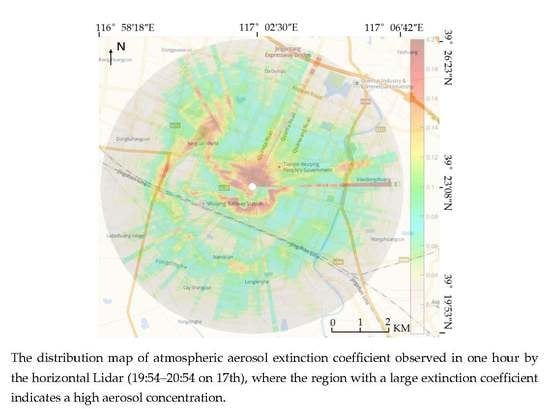
The horizontal distribution of the aerosol was detected by the horizontal scanning LiDAR positioned at the top of the residential building. The single scan time was set to 20 s, the scan step angle was 2°, the horizontal direction scan could be finished in 1 hour, and the clockwise rotation was continuously scanned from the north direction to ensure the signal-to-noise ratio. Extinction coefficient retrieval was performed by the proposed horizontal retrieval algorithm. Figure 6a shows a distribution map of the atmospheric aerosol extinction coefficient observed in one hour in the horizontal direction (19:54–20:54 on 17 August), where the region with a large extinction coefficient indicates a high aerosol concentration. During this period, the aerosol pollution was mainly concentrated within 1 km of the observation point and a band of contaminated area with high concentration was observed in the direction of the northwest.
Figure 6b shows the fused results after 24 h of consecutive observations. This figure reflects the distribution of heavily polluted areas in the area within 24 h. The method adopted involved the extraction of aerosol data in highly polluted areas, removal of low pollution parts, and fusion of these parts into a single map. Six heavily polluted areas were observed on 17 August 2018. According to field investigation, area 1 is an industrial area and industrial activities were the main cause of high aerosol concentration. Areas 2 to 6 are densely populated and have heavy traffic. Industrial production, living, and transportation were the main causes of high aerosol concentration in these regions.
Comparing the results in Figure 3 and Figure 6b, the source of local pollutants in Wuqing District on 17 August 2018 was mainly the areas with serious pollution seen in Figure 6b. For the meteorological data, the wind in Wuqing District blows from north or northeast at a speed of level 1 to 3. Therefore, industrial area 1 may be one of the main sources of pollutants.
Under normal circumstances, the aerosol extinction coefficient cannot be directly converted to absolute particle mass concentration; however, there is evidence showing that a certain linear relationship exists between the particle concentration and the extinction coefficient obtained by LiDAR detection [41]. Fitting research and correlation analysis between the LiDAR horizontal scanning results and the ground station hourly averaged PM10 data, as well as PM2.5, were conducted to initially verify the accuracy of LiDAR detection results. The fitting results are shown in Figure 7. The aerosol extinction coefficients of the horizontal LiDAR in Figure 7 are the LiDAR results at the position of the air quality national control station (point C in Figure 1). We set the single data integration time as 20 s and the step angle as 2°, thus a complete scan took one hour. Therefore, we believed that the aerosol extinction coefficient at such point was also hourly averaged.
The empirical fitting formula for the PM10 concentration and the retrieved aerosol extinction coefficient is as follows:
where Y is the PM10 particle concentration in μg/m3 and X is the aerosol extinction coefficient observed by horizontal LiDAR in the unit of km−1.
Y = 499.63 × X + 5.78,
The goodness of fit between the aerosol extinction coefficient and the PM10 concentration monitored by the air quality national control station was 0.84, and the number of samples was N = 334, collected in 14 days. As for PM2.5, the goodness of linear fit was 0.69, which was less than that of PM10. Thus, we believe that, in this experiment, the fitting result of PM10 shows a relatively high degree of linearity. Therefore, the LiDAR can be utilized when obtaining the empirical formula for a certain time period, and the horizontal distribution map of the aerosol extinction coefficient detected by the LiDAR can directly reflect concentration of the particulate matter, especially for PM10, in the scanning area.
5. Discussion
For a more comprehensive analysis, we added the satellite remote sensing monitoring results and backward trajectory model analysis. The satellite remote sensing data used in this paper was the hourly observation data of surface PM2.5 concentration of the Himawari-8 satellite in Jing-Jin-Ji area, China, from 15–19 August 2018 [42]. The hourly surface PM2.5 mass concentrations were obtained from the official website of the China Environmental Monitoring Center (CEMC: http://106.37.208.233:20035). Satellite remote sensing monitoring has the advantage of wide coverage and can use large-scale satellite remote sensing to scan the distribution of atmospheric pollutants and determine the overall diffusion trend of pollutants [43,44,45]. According to the backward trajectory model and monitoring results, the pollution source in Wuqing District could be determined as an extraterritorial pollution source or a pollution source within the domain.
Figure 8 shows the spatial distribution of PM2.5 daily concentration of fine particulate matter retrieved from satellite remote sensing monitoring data from 15–19 August 2018. The blue marked area is Wuqing District, Tianjin. The PM2.5 pollution level in the entire Jing-Jin-Ji region, including Wuqing District, was low from 15–16 August. On 17 August, slight pollution was observed in the north of the Jing-Jin-Ji region and was further strengthened on 18 August, resulting in the two heavily polluted areas centered on Shijiazhuang City and Tangshan City and increased pollution level in Wuqing District. On 19 August 19, the PM2.5 pollution level in the Jing-Jin-Ji region significantly decreased.
Figure 9 shows the distribution of the daily trajectory of the air mass from 15–19 August 2018, in Wuqing District, Tianjin. The backward trajectory model we mentioned in this paper was generated by using the HYSPLIT-4 model [46]. It was developed by the National Oceanic and Atmospheric Administration. This model simulation uses 1° × 1° global meteorological data from the NCEP Global Data Assimilation System. On 15 August, the near-surface air mass route to Wuqing District was from Inner Mongolia, Liaoning, and other places. The high-rise air masses originated from the Bohai Sea and the Yellow Sea. Therefore, the main airflow to Wuqing was clean air. On 16 to 17 August, the air mass reached the Wuqing through long-distance transportation and passed through Heilongjiang, Liaoning, and other places, affecting the air quality in the northern part of Beijing, Tianjin, and Hebei to some extent. On 18 August, the air mass was mainly from the interior of the Jing-Jin-Ji region and was introduced into Wuqing from the northeast, resulting in the accumulation of fine particulate pollutants in the area. On 19 August, the air masses arriving in Wuqing originated from the adjacent Bohai Sea and the Yellow Sea. The clean air flow improved the air quality in Wuqing District and the entire Jing-Jin-Ji region.
The results from of Figure 3a, Figure 4, Figure 5, Figure 6 and Figure 8 and Figure 9 indicate that the particulate matter pollutants affecting the air quality of Wuqing District on the 15–19 August were mainly generated by local sources, including pollution from the production of residents, life, transportation, and industrial production activities.
6. Conclusions
This study observed the atmospheric aerosol pollution in Wuqing District through the integration of sky and ground measurement (LiDAR, satellite, and ground observation station) and combined the backward trajectory model trace to reveal the vertical and horizontal distribution characteristics and provide some evidence of potential sources of the aerosol pollution in the area. The calibration and correlation fitting analysis of the particulate matter data of the ground air quality national control station showed that LiDAR can effectively detect atmospheric aerosol pollution.
- On 17–19 August 2018, the particulate matter pollutants in Wuqing District were mainly from the local area. The particulate matter mainly accumulated at 2.0 km and the boundary layer height also changed around 1 to 2 km.
- The distribution of aerosol pollution in the scanning area was obtained by using the horizontal scanning LiDAR positioned on the top of a building to obtain the horizontal distribution result of aerosol.
- Using the LiDAR network observation and combining the satellite and ground-integrated observation mode in a certain area was conducive to the study of the regional distribution characteristics of pollutants and the cross-boundary transport of pollutant air masses. Providing reliable data support for regional atmospheric defense joint control policies and means was also beneficial to this study.
Author Contributions
Methodology, C.W. and Y.M.; Supervision, W.G.; Validation, G.H., S.L., and J.C.; Writing—original draft, X.M. All authors read the manuscript, contributed to the discussion, and gave valuable suggestions to improve the manuscript.
Funding
This work was partially supported by the National Natural Science Foundation of China [Grant numbers 41801261, 41827801, 41601351]; the National Key Research and Development Program of China [Grant number 2017YFC0212600]; Postdoctoral Science Foundation of China [Grant numbers 2017T100580, 2016M602362, 2016M600612]; the National Science and Technology Major Project [Grant numbers 11-Y20A12-9001-17/18, 42-Y20A11-9001-17/18]; the LIESMARS Special Research Funding.
Conflicts of Interest
The authors declare no conflict of interest.
References
- Pöschl, U. Atmospheric aerosols: Composition, transformation, climate and health effects. Angew. Chem. Int. Ed. 2005, 44, 7520–7540. [Google Scholar] [CrossRef] [PubMed]
- Heal, M.R.; Kumar, P.; Harrison, R.M. Particles, air quality, policy and health. Chem. Soc. Rev. 2012, 41, 6606–6630. [Google Scholar] [CrossRef] [PubMed] [Green Version]
- Kampa, M.; Castanas, E. Human health effects of air pollution. Environ. Pollut. 2008, 151, 362–367. [Google Scholar] [CrossRef] [PubMed]
- Vandyck, T.; Keramidas, K.; Kitous, A.; Spadaro, J.V.; Van Dingenen, R.; Holland, M.; Saveyn, B. Air quality co-benefits for human health and agriculture counterbalance costs to meet Paris Agreement pledges. Nat. Commun. 2018, 9, 4939. [Google Scholar] [CrossRef] [PubMed]
- Zhang, Q.; Jiang, X.; Tong, D.; Davis, S.J.; Zhao, H.; Geng, G.; Feng, T.; Zheng, B.; Lu, Z.; Streets, D.G. Transboundary health impacts of transported global air pollution and international trade. Nature 2017, 543, 705–709. [Google Scholar] [CrossRef] [PubMed] [Green Version]
- Chan, K.L.; Wiegner, M.; Flentje, H.; Mattis, I.; Wagner, F.; Gasteiger, J.; Geiß, A. Evaluation of ECMWF-IFS (version 41R1) operational model forecasts of aerosol transport by using ceilometer network measurements. Geosci. Model Dev. 2018, 11, 3807–3831. [Google Scholar] [CrossRef] [Green Version]
- Huang, R.-J.; Zhang, Y.; Bozzetti, C.; Ho, K.-F.; Cao, J.-J.; Han, Y.; Daellenbach, K.R.; Slowik, J.G.; Platt, S.M.; Canonaco, F. High secondary aerosol contribution to particulate pollution during haze events in China. Nature 2014, 514, 218–222. [Google Scholar] [CrossRef] [Green Version]
- Guo, S.; Hu, M.; Zamora, M.L.; Peng, J.; Shang, D.; Zheng, J.; Du, Z.; Wu, Z.; Shao, M.; Zeng, L. Elucidating severe urban haze formation in China. Proc. Natl. Acad. Sci. USA 2014, 111, 17373–17378. [Google Scholar] [CrossRef] [Green Version]
- Wang, Y.; Yao, L.; Wang, L.; Liu, Z.; Ji, D.; Tang, G.; Zhang, J.; Sun, Y.; Hu, B.; Xin, J. Mechanism for the formation of the January 2013 heavy haze pollution episode over central and eastern China. Sci. China Earth Sci. 2014, 57, 14–25. [Google Scholar] [CrossRef]
- Chan, K. Biomass burning sources and their contributions to the local air quality in Hong Kong. Sci. Total Environ. 2017, 596, 212–221. [Google Scholar] [CrossRef]
- Chan, K. Aerosol optical depths and their contributing sources in Taiwan. Atmos. Environ. 2017, 148, 364–375. [Google Scholar] [CrossRef]
- Xing, C.; Liu, C.; Wang, S.; Chan, K.; Gao, Y.; Huang, X.; Su, W.; Zhang, C.; Dong, Y.; Fan, G. Observations of the summertime atmospheric pollutants vertical distributions and the corresponding ozone production in Shanghai, China. Atmos. Chem. Phys. Discuss. 2017, 2017, 14275–14289. [Google Scholar] [CrossRef]
- Taylor, M.; Retalis, A.; Flocas, H.A. Particulate matter estimation from photochemistry: A modelling approach using neural networks and synoptic clustering. Aerosol Air Qual. Res. 2016, 16, 2067–2084. [Google Scholar] [CrossRef]
- Han, G.; Xu, H.; Gong, W.; Liu, J.; Du, J.; Ma, X.; Liang, A. Feasibility Study on Measuring Atmospheric CO2 in Urban Areas by Using Spaceborne CO2-IPDA LIDAR. Remote Sens. 2018, 10, 985. [Google Scholar] [CrossRef]
- Han, G.; Ma, X.; Liang, A.; Zhang, T.; Zhao, Y.; Zhang, M.; Gong, W. Performance Evaluation for China’s Planned CO2-IPDA. Remote Sens. 2017, 9, 768. [Google Scholar] [CrossRef]
- Dong, Y.; Du, B.; Zhang, L.; Hu, X. Hyperspectral Target Detection via Adaptive Information-Theoretic Metric Learning with Local Constraints. Remote Sens. 2018, 10, 1415. [Google Scholar] [CrossRef]
- Dong, Y.; Du, B.; Zhang, L.; Zhang, L. Dimensionality Reduction and Classification of Hyperspectral Images Using Ensemble Discriminative Local Metric Learning. IEEE Trans. Geosci. Remote Sens. 2017, 55, 2509–2524. [Google Scholar] [CrossRef]
- Ma, X.; Shi, T.; Xu, H.; He, B.; Qiu, R.; Han, G.; Gong, W. On-line wavenumber optimization for a ground-based CH4-DIAL. J. Quant. Spectrosc. Radiat. Transf. 2019, 229, 106–119. [Google Scholar] [CrossRef]
- Dai, G.; Wu, S.; Song, X. Depolarization ratio profiles calibration and observations of aerosol and cloud in the Tibetan Plateau based on polarization Raman lidar. Remote Sens. 2018, 10, 378. [Google Scholar] [CrossRef]
- Mao, F.; Liu, J.; Wang, L.; Chen, S.; Li, C. Denoising and retrieval algorithm based on a dual ensemble Kalman filter for elastic lidar data. Opt. Commun. 2019, 433, 137–143. [Google Scholar] [CrossRef]
- Sun, T.; Che, H.; Qi, B.; Wang, Y.; Dong, Y.; Xia, X.; Wang, H.; Gui, K.; Zheng, Y.; Zhao, H. Characterization of vertical distribution and radiative forcing of ambient aerosol over the Yangtze River Delta during 2013–2015. Sci. Total Environ. 2019, 650, 1846–1857. [Google Scholar] [CrossRef] [PubMed]
- Matthias, V.; Balis, D.; Bösenberg, J.; Eixmann, R.; Iarlori, M.; Komguem, L.; Mattis, I.; Papayannis, A.; Pappalardo, G.; Perrone, M. Vertical aerosol distribution over Europe: Statistical analysis of Raman lidar data from 10 European Aerosol Research Lidar Network (EARLINET) stations. J. Geophys. Res. Atmos. 2004, 109. [Google Scholar] [CrossRef]
- Niranjan, K.; Sreekanth, V.; Madhavan, B.; Krishna Moorthy, K. Wintertime aerosol characteristics at a north Indian site Kharagpur in the Indo-Gangetic plains located at the outflow region into Bay of Bengal. J. Geophys. Res. Atmos. 2006, 111. [Google Scholar] [CrossRef] [Green Version]
- Xia, H.; Shentu, G.; Shangguan, M.; Xia, X.; Jia, X.; Wang, C.; Zhang, J.; Pelc, J.S.; Fejer, M.; Zhang, Q. Long-range micro-pulse aerosol lidar at 1.5 μm with an upconversion single-photon detector. Opt. Lett. 2015, 40, 1579–1582. [Google Scholar] [CrossRef] [PubMed]
- Lu, X.; Li, X.; Qin, W.; Cui, S.; Liu, Q.; Xu, Q. Retrieval of horizontal distribution of aerosol mass concentration by micro pulse lidar. Opt. Precis. Eng. 2017, 25, 1697–1704. [Google Scholar]
- Lv, Y.; Li, Z.; Xie, J.; Zhang, F.; Liu, X.; Liu, Z.; Xie, Y.; Xu, H.; Chen, X. Monitoring the distributed point pollution sources based on a scanning Lidar. China Environ. Sci. 2017, 37, 4078–4084. [Google Scholar]
- Xian, J.; Han, Y.; Huang, S.; Sun, D.; Zheng, J.; Han, F.; Zhou, A.; Yang, S.; Xu, W.; Song, Q. Novel Lidar algorithm for horizontal visibility measurement and sea fog monitoring. Opt. Express 2018, 26, 34853–34863. [Google Scholar] [CrossRef] [PubMed]
- Zeng, X.; Xia, M.; Ge, Y.; Guo, W.; Yang, K. On-site ocean horizontal aerosol extinction coefficient inversion under different weather conditions on the Bo-hai and Huang-hai Seas. Atmos. Environ. 2018, 177, 18–27. [Google Scholar] [CrossRef]
- Bo, G.; Xu, C.; Li, A.; Wang, Y.; Chen, H.; Jiang, Y. Optical and hygroscopic properties of Asian dust particles based on a horizontal Mie lidar: Case study at Hefei, China. Chin. Opt. Lett. 2017, 15, 020102. [Google Scholar]
- Zhang, M.; Wang, L.; Bilal, M.; Gong, W.; Zhang, Z.; Guo, G. The Characteristics of the Aerosol Optical Depth within the Lowest Aerosol Layer over the Tibetan Plateau from 2007 to 2014. Remote Sens. 2018, 10, 696. [Google Scholar] [CrossRef]
- Lee, K.H.; Wong, M.S. Vertical Profiling of Aerosol Optical Properties From LIDAR Remote Sensing, Surface Visibility, and Columnar Extinction Measurements. Remote Sensing of Aerosols, Clouds, and Precipitation; Academic Press, Elsevier: Amsterdam, The Netherlands, 2018; pp. 23–43. [Google Scholar]
- Liu, D.; Zhao, T.; Boiyo, R.; Chen, S.; Lu, Z.; Wu, Y.; Zhao, Y. Vertical Structures of Dust Aerosols over East Asia Based on CALIPSO Retrievals. Remote Sens. 2019, 11, 701. [Google Scholar] [CrossRef]
- Kaestner, M. Lidar inversion with variable backscatter/extinction ratios: Comment. Appl. Opt. 1986, 25, 833–835. [Google Scholar] [CrossRef] [PubMed]
- Klett, J.D. Lidar inversion with variable backscatter/extinction ratios. Appl. Opt. 1985, 24, 1638–1643. [Google Scholar] [CrossRef] [PubMed]
- Klett, J.D. Stable analytical inversion solution for processing lidar returns. Appl. Opt. 1981, 20, 211–220. [Google Scholar] [CrossRef] [PubMed] [Green Version]
- Fernald, F.G. Analysis of atmospheric lidar observations: Some comments. Appl. Opt. 1984, 23, 652–653. [Google Scholar] [CrossRef] [PubMed]
- Kunz, G.J.; de Leeuw, G. Inversion of lidar signals with the slope method. Appl. Opt. 1993, 32, 3249–3256. [Google Scholar] [CrossRef] [PubMed]
- Sasano, Y.; Nakane, H. Significance of the extinction/backscatter ratio and the boundary value term in the solution for the two-component lidar equation. Appl. Opt. 1984, 23, 11–13. [Google Scholar] [CrossRef] [PubMed]
- Jorg, A. The extinction-to-backscatter ratio of tropospheric aerosol: A numerical study. J. Atmos. Ocean. Technol. 1998, 15, 1043–1050. [Google Scholar]
- Pan, Y.; Lu, D.; Pan, W. A New Method for Aerosol Retrieval Based on Lidar Observations in Beijing. Atmos. Ocean. Sci. Lett. 2014, 7, 203–209. [Google Scholar]
- Miffre, A.; Chacra, M.; Geffroy, S. Aerosol load study in urban area by Lidar and numerical model. Atmos. Environ. 2010, 44, 1152–1161. [Google Scholar] [CrossRef]
- Wang, W.; Mao, F.; Du, L.; Pan, Z.; Gong, W.; Fang, S. Deriving hourly PM2.5 concentrations from himawari-8 aods over beijing–tianjin–hebei in China. Remote Sens. 2017, 9, 858. [Google Scholar] [CrossRef]
- Wang, Y.; Wang, Z.; Yu, C.; Zhu, S.; Cheng, L.; Zhang, Y.; Chen, L. Validation of OMI HCHO Products Using MAX-DOAS observations from 2010 to 2016 in Xianghe, Beijing: Investigation of the Effects of Aerosols on Satellite Products. Remote Sens. 2019, 11, 203. [Google Scholar] [CrossRef]
- Pan, Z.; Mao, F.; Wang, W.; Logan, T.; Hong, J. Examining Intrinsic Aerosol-Cloud Interactions in South Asia Through Multiple Satellite Observations. J. Geophys. Res. Atmos. 2018, 123, 11–210. [Google Scholar] [CrossRef]
- Zang, L.; Mao, F.; Guo, J.; Wang, W.; Pan, Z.; Shen, H.; Zhu, B.; Wang, Z. Estimation of spatiotemporal PM1.0 distributions in China by combining PM2.5 observations with satellite aerosol optical depth. Sci. Total Environ. 2019, 658, 1256–1264. [Google Scholar] [CrossRef] [PubMed]
- Lu, X.; Mao, F.; Pan, Z.; Gong, W.; Wang, W.; Tian, L.; Fang, S. Three-dimensional physical and optical characteristics of aerosols over central China from long-term CALIPSO and HYSPLIT Data. Remote Sens. 2018, 10, 314. [Google Scholar] [CrossRef]
Figure 1.
Distribution of the two LiDARs (light detection and ranging) and the air quality national control station. The base map in the satellite figure is a high-definition map. The red dots A, B, and C are the locations of the horizontal LiDAR, the vertical LiDAR, and the air quality national control station, respectively. The distance between A and B is 752 m. The distance between B and C is 803 m. The distance between A and C is 1147 m.

Figure 2.
Flow chart of the retrieval method for the horizontal light detection and ranging (LiDAR) signal.
Figure 2.
Flow chart of the retrieval method for the horizontal light detection and ranging (LiDAR) signal.

Figure 3.
(a) Aerosol extinction coefficient results for 24-hour continuous vertical observation by light detection and ranging (LiDAR) on 15–19 August 2018. (b) Hourly averaged AOD (Aerosol Optical Depth) observed by LiDAR on 15–19 August 2018.
Figure 3.
(a) Aerosol extinction coefficient results for 24-hour continuous vertical observation by light detection and ranging (LiDAR) on 15–19 August 2018. (b) Hourly averaged AOD (Aerosol Optical Depth) observed by LiDAR on 15–19 August 2018.


Figure 4.
Hourly averaged PM10 and PM2.5 (particulate matter) observed by the air quality national control station on 15–19 August 2018.
Figure 4.
Hourly averaged PM10 and PM2.5 (particulate matter) observed by the air quality national control station on 15–19 August 2018.

Figure 5.
The wind rose of Wuqing District on 15–19 August 2018.

Figure 6.
Aerosol extinction coefficient detected by the horizontal light detection and ranging (LiDAR). The top figure (a)—aerosol extinction coefficient detection result by horizontal LiDAR scanning in one hour—illustrates the results covering an area with a radius of 5 km after one hour of continuous observation, and the bottom figure (b)—aerosol extinction coefficient fused results in 24 h—shows the fused results highlighting areas with heavy pollution.

Figure 7.
Linear fitting relationship between the aerosol extinction coefficient with PM10 and PM2.5 concentrations monitored by the air quality national control station in 14 days, respectively. The black squares represent PM10 and the red dots represent the PM2.5. PM: particulate matter.
Figure 7.
Linear fitting relationship between the aerosol extinction coefficient with PM10 and PM2.5 concentrations monitored by the air quality national control station in 14 days, respectively. The black squares represent PM10 and the red dots represent the PM2.5. PM: particulate matter.

Figure 8.
Spatial distribution of fine particulate PM2.5 concentration in Beijing-Tianjin-Hebei region from 15–19 August (daytime) 2018. PM: particulate matter.
Figure 8.
Spatial distribution of fine particulate PM2.5 concentration in Beijing-Tianjin-Hebei region from 15–19 August (daytime) 2018. PM: particulate matter.


Figure 9.
Backward trajectory map of the Wuqing District of Tianjin from 15–19 August 2018.


Table 1.
Technical parameters of the two light detection and ranging (LiDARs).
| Parameter | Vertical LiDAR | Horizontal LiDAR |
|---|---|---|
| Wavelength | 1064 nm | 1064 nm |
| Pulse energy | >100 μJ | >20 μJ |
| Pulse repetition frequency | 2.5 kHz | 10 kHz |
| Telescope diameter | 100 mm | 100 mm |
| FOV | <1 mrad | <0.2 mrad |
| Range resolution | 30 m | 15 m |
| Detection blind zone | 100 m | 150 m |
LiDAR: Light Detection and Ranging; FOV: Field of View.
© 2019 by the authors. Licensee MDPI, Basel, Switzerland. This article is an open access article distributed under the terms and conditions of the Creative Commons Attribution (CC BY) license (http://creativecommons.org/licenses/by/4.0/).
Share and Cite
MDPI and ACS Style
Ma, X.; Wang, C.; Han, G.; Ma, Y.; Li, S.; Gong, W.; Chen, J. Regional Atmospheric Aerosol Pollution Detection Based on LiDAR Remote Sensing. Remote Sens. 2019, 11, 2339. https://doi.org/10.3390/rs11202339
AMA Style
Ma X, Wang C, Han G, Ma Y, Li S, Gong W, Chen J. Regional Atmospheric Aerosol Pollution Detection Based on LiDAR Remote Sensing. Remote Sensing. 2019; 11(20):2339. https://doi.org/10.3390/rs11202339
Chicago/Turabian StyleMa, Xin, Chengyi Wang, Ge Han, Yue Ma, Song Li, Wei Gong, and Jialin Chen. 2019. "Regional Atmospheric Aerosol Pollution Detection Based on LiDAR Remote Sensing" Remote Sensing 11, no. 20: 2339. https://doi.org/10.3390/rs11202339
Note that from the first issue of 2016, this journal uses article numbers instead of page numbers. See further details here.