Removal of Covariant Errors from Altimetric Wave Height Data


EOSA, Plymouth Marine Laboratory, Plymouth PL1 3DH, UK
Remote Sens. 2019, 11(19), 2319; https://doi.org/10.3390/rs11192319
Submission received: 2 September 2019
/
Revised: 27 September 2019
/
Accepted: 3 October 2019
/
Published: 5 October 2019
(This article belongs to the Section Ocean Remote Sensing)
Abstract
:The echo waveforms received by conventional radar altimeters are interpreted by retracking algorithms to give estimates of range, wave height, and backscatter strength. However, in response to fading noise on the waveform leading edge, common retrackers, such as MLE-3 and MLE-4, show correlated errors in wave height and range. This correlation is used to develop a correction to the wave height data that reduces the high-frequency variability by ∼22%, without affecting the global distribution of values. This correction also results in a closer matchup of Jason-2 and Jason-3 data during their tandem phase. Although the correction is quite straightforward in practice, the appropriate conversion factor has to be determined for each combination of altimeter and retracker. There are also remaining open questions concerning the needed low-pass filtering.
1. Introduction
There are now more than three decades of near-continuous wave height data from satellites, which have been used to describe the regional wave climate and its trends [1]. Altimeter data can also be used to give the broad scale picture across storms, and for ingestion into wave forecasting models. However, wave height data from altimeters are less frequently analysed at their finer scale because of short-scale noise within the data records. We investigate how these data can be improved to potentially enable studies of wave–current interaction and better comparisons between different altimeters and with wave buoys.
Satellite-borne radar altimeters are principally designed to accurately record range information (in order to determine sea level), but their return signals are also widely interpreted to give significant wave height (SWH) and wind speed, and information on other atmospheric or oceanic conditions [2]. Most radar altimeters to date have been “low resolution measurement“ (LRM), with the only information recorded being the time series of power level within the radar echo. Instruments operating in this LRM mode typically produce signals as illustrated in Figure 1a. The expected signal has a simple functional form (Figure 1b), corresponding to the mathematical convolution of three terms [3,4]. However, the signal received is beset by “fading noise“ in that the vector summation from multiple small reflecting facets on the sea surface will have a mean power, P, as shown in Figure 1b, but with a random variation governed by statistics such that the standard deviation (S.D.) of multiple realizations is , where N is the number of independent pulses averaged. As the instrument sampling permits only a limited number of pulses to be averaged, this fading noise will be present in all signals analysed. Consequently, algorithms designed to fit a model waveform to the observations and to derive its key parameters must be designed to minimise their sensitivity to this noise term. A number of these “retracker“ algorithms are commonly used, including MLE-4 [5] and ALES [6].
Several papers have shown that there is “cross-talk“ between the estimation of wave height (Hs) and range, as both are derived from information on the leading edge, and thus a particular realization of fading noise can lead to covariant errors in these two terms. Similarly, for those algorithms that fit both amplitude () and mispointing (), which are both terms related to the power distribution in the trailing edge (see Figure 1b), there is a strong connection between their errors [7,8]. Quartly [7] showed how this property could be used to significantly improve the estimates from the MLE-4 algorithm and, more recently, Zaron and deCarvalho [9] and then Quartly et al. [10] have demonstrated how the Hs data can be utilised to provide smoother (more realistic) variations in range, and thus ultimately in sea level. Here, we take those ideas and explore the potential for the range information to be used instead to improve the quality of wave height estimates.
In the majority of waveform-fitting algorithms, the slope of the leading edge is governed by a term , which combines the effect of the width of the emitted pulse, and of the spread of reflecting facets governed by significant wave height, Hs:
where and are expressed in travel time and c is the speed of light. On occasions, the random fading noise may result in a steeper leading edge than would be expected for a flat surface, i.e., . Often in such circumstances, the derived estimate for Hs is set to zero, potentially leading to multiple neighbouring values being the same, resulting in a spike in the probability distribution function, and an unreasonably low estimate of the variability within a 1 Hz record (denoted ). Alternate coding of the information is possible, whereby the Hs value reflects the fact that was less than its theoretical minimum.
2. Covariant Errors of Properties of Leading Edge
In simulation work, involving a retracker algorithm applied to a waveform with appropriate fading noise, Sandwell and Smith [11] had shown there was a very strong correlation between the errors in the derived slope and in the epoch (position of the mid-power point). In their work, the error was well-defined since the true position without noise was known. In a practical implementation neither the true epoch nor the range is known, so we approximate this by the anomaly about the local mean. In a preliminary study, Smith et al. [12] examined the cross-spectra of sea surface height and SWH, noting that the magnitude squared coherence (equivalent to the correlation coefficient, ) was high (around 0.4) for all scales smaller than 50 km. These results have been corroborated more recently by Tran et al. [13] in a detailed analysis of the MLE-4 retracker (4-parameter Maximum Likelihood Estimator) on Jason-3.
We explore the potential for improving the quality of altimeter wave height data through reducing these covariant errors, applying our ideas to Jason-3 products from both MLE-4 and MLE-3 retrackers (the latter not fitting the 4th term, ). For practical purposes, we use = altitude minus range, ignoring all the geophysical and instrumental corrections that vary on scales >50 km.
To examine the covariant properties, we consider individual 1-second records of data, containing twenty 20 Hz measurements. These correspond to overlapping circular footprints between 2 and 10 km in diameter depending upon wave height [14,15], but spaced at intervals of 330 m along track—thus, there should be minimal real physical change between neighbouring data points. Following Quartly et al. [10], we detrend both the and Hs measurements to emphasise the high-frequency variations which are due to the fading noise. In their work, they determined , the slope of the red line in Figure 2a governing the portion of anomaly explained by SWH anomaly. Here, we perform the regression the other way (corresponding to the green line) to give the proportionality value, , indicating how the anomaly affects Hs. (Clearly, if the two parameters were perfectly correlated, then would be the reciprocal of .)
We calculate the slope of the relationship for all fully marine 1 Hz records having a full complement of 20 observations. (To obtain data on the covariance due to fading noise alone, we avoid contamination by land, ice, and rain by using, respectively, thresholds on proximity to land, latitude outside polar regions, and negligible differential attenuation between its two radar frequencies.) Individual 1-second ensembles will yield a wide range of values for and the associated statistic detailing the fraction of variance explained. Figure 3a shows that the spread of values for is indicated by the 5th and 95th percentiles of the distribution, but the median value is close to −4 for a wide range of Hs values, although with significant change at low sea states. The median value is typically greater than 0.40 (Figure 3c), with an increase at low sea states. The analysis of the output of the MLE-3 retracker yields a similar distribution for , as did MLE-4, but the values of explained variance are slightly lower.
As the composite width, , is the variable that best describes the width of the leading edge (rather than Hs), we perform a similar analysis linking anomalies in to those in (Figure 2b) and noting how its relationship varies with Hs (Figure 3b). For large wave heights (Hs > 2m), approximates to , and thus the regression statistics show the same value with the derived values differing by a factor of 1.67 (if Hs is in metres and in nanoseconds). The curves differ at low Hs, where Equation (1) is nonlinear, but the utilization of does not give a much simpler form.
3. Implementation of SWH Adjustment and Its Evaluation
This understanding of the covariant errors can be used to implement an empirical adjustment to the default Hs estimates:
where and are the original and adjusted estimates of wave height, and is the local anomaly in . To enable a continuous correction over large segments of data, we calculate relative to a running 21-point median, viz:
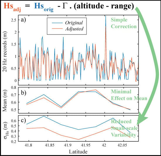
Within our implementation (Figure 4), the appropriate adjustment factor, , could be defined from Figure 3a, based on an average Hs value for that segment, although that approach is slightly circular given that Hs is the parameter to be improved. For simplicity, here we use the mean value () in all circumstances (and for the MLE-3 retracker); the Appendix shows that there is minimal benefit (in this particular case) in implementing a lookup table characterizing as a function of Hs. Figure 5 shows an example of the effective improvement in 20 Hz Hs data—the top panel shows the change for individual values, whilst the middle panel shows that the mean is little affected, since the mean of 20 consecutive records of is close to zero. Figure 5c quantifies how much the variability is reduced for this example.
The global view of this reduction in variability is illustrated in Figure 6. The left-hand panel illustrates the probability distribution function of for 300 Jason-3 tracks (∼12 days), with this measure of variability only tallied when present for all four retrackers (MLE-4 and MLE-3 on the GDR, and the “adjusted“ versions of each). The distributions for “adjusted MLE-4“ and “adjusted MLE-3“ almost coincide, but the latter does have more large values ( m). The median value for each retracker is highlighted by the solid vertical lines: 0.534 m for MLE-4, 0.511 m for MLE-3, and 0.405 m for both adjusted versions, corresponding to changes in of 24% and 21% respectively, and thus reductions in variance of about 40%. The dashed lines show the 95th percentiles, as these are sometimes used as a threshold for discarding unreliable data. Variability in Hs estimates is known to be greater in high wave height conditions, suggesting that the flagging of Hs data based on should be done using a threshold that varies with Hs—Figure 6b shows this variation to be common to both MLE-4 and MLE-3 retrackers and the adjusted versions of them. (Large values of coherence between range and Hs have been reported at all scales below ∼50 km [12,13], so we have investigated calculating relative to a 101-point running median filter, corresponding to ∼33 km along track. However, the results were not appreciably different.)
A further validation of the usefulness of this adjustment is provided in Figure 7, which matches up the 20 Hz records of Jason-2 and Jason-3 data during the tandem phase at the beginning of Jason-3’s mission. The two satellites were flying along the same ground track, with Jason-2 between 81 and 83 s ahead of Jason-3, and the match-ups agree in latitude to within 0.001. The mean offset between the two (blue line in Figure 6a) shows some variation with Hs (most noticeably below 1.5 m). The spread of values in their difference is shown by the standard deviation (Figure 7b)—the values for MLE-4 are consistent with times the variability for one instrument (Figure 6b). Implementing the adjustment for both Jason-2 and Jason-3 has negligible impact on the mean offset between the two instruments, but reduces the S.D. of the differences by ∼22%.
Similar to the analysis for improving and sea surface heights () data [10], the pertinent value of will vary with both altimeter and retracker applied. Figure 8 provides a synopsis of similar analysis for MLE-4 processing of data from AltiKa, the Ka-band altimeter on the SARAL spacecraft. That altimeter produces 40 average waveforms and thus 40 separate estimates of the parameters per second [16]—individual 1-second ensembles from 500 passes (∼17.5 days) are used to determine the appropriate value of and the associated . In this case, the median value of is −5.06, slightly larger in magnitude than for Jason-3. It also has a more marked variation at low Hs, suggesting that implementation using a variable may be beneficial. The median value is 0.44, slightly higher than that for Jason-3. Implementation of an adjustment, simply using the mean value of and the anomaly relative to a 41-point (1-second) running median, leads to a significant reduction in the values, with the median value reducing by 18% from 0.33 m to 0.27 m.
4. Conclusion and Discussion
Since both estimates of range and wave height are derived from a few waveform bins on the leading edge of an LRM waveform, their estimates are sensitive to the existence of fading noise affecting the power levels within this section of the waveform (Figure 1b). Sandwell and Smith [11] showed that there was a correlation between the noise-induced anomalies in these two parameters, and Zaron and deCarvalho [9] and Quartly et al. [10] have used this empirical connection to reduce the errors in range. The present paper demonstrates that the reverse procedure is equally applicable: using local anomalies in (altitude minus range) to reduce the associated errors in SWH.
The coefficient, , linking the anomalies in these two terms is found to vary slightly with Hs, with the nonuniformity being most marked for Hs < 1.5 m (Figure 3a)—recasting the empirical link so as to be between and (a term better describing the width of the waveform leading edge) did not improve this (Figure 3c). As noted for the analysis on improving and [10], the coefficient to improve Hs depends upon both the altimeter and the retracking algorithm used. The appropriate values of for MLE-4 and MLE-3 are very similar, whereas a different value is needed for ALES applied to Jason data (not shown). In the same way, MLE-4 applied to AltiKa data needs a different value (see Figure 8a). This paper only shows results for LRM altimeters. A brief analysis has been carried out for Sentinel-3 when the altimeter was operating in SAR mode, and the reduction in variance was much smaller than for LRM operations [17]. This is because the SAR waveform has a different shape, with a sharp drop in the trailing edge that depends upon wave height (see Figure 9b of Ardhuin et al. [18])—as more waveform bins are sensitive to Hs, the noise level on its initial estimate is lower, with less cross-talk with the range estimate, which is in effect only extracted from the SAR waveform’s leading edge.
In this paper, we demonstrated the implementation of an “adjustment“ to Hs using a constant value of as an approximation to the variation shown in Figure 3a. In a similar analysis, which only focused on MLE-4 applied to Jason-3, Tran et al. [13] modelled the variation as a simple linear function of Hs. With their adjustment, they achieved a reduction in of 38% at Hs = 2 m, which is larger than the 22% achieved here (see Figure 6, for example). Their analysis used altitude minus range minus mean sea surface, with that field smoothed by a low-pass Lanczos filter of width 140 km, i.e., ∼20 times broader than that implemented here, and also showed a significant reduction in SWH spectra for all wavelengths up to 70 km. However, the results in the present paper showed negligible change when the width of the median filter was changed from 21 to 101 points. Possibly their inclusion of a detailed mean sea surface (MSS) has removed stationary anomalies not associated with the effect of fading noise. Thus, the importance of incorporating MSS may need to be evaluated in the future.
A further demonstration of the efficacy of the proposed adjustment was the improved agreement between two independent (but very similar) altimeter systems. With adjustments to the Hs values for both Jason-2 and Jason-3, the S.D. of the discrepancy between the two reduces by ∼22%, in line with the change in estimated noise for one instrument. Note that as the two follow the same track within a very narrow deadband, the effect of omitting the MSS term should be similar for both instruments.
The advocated procedure removes an error contribution associated with the retracking of fading noise. Other sources of error will remain, so this adjustment may be combined with along-track smoothing or empirical mode decomposition [19] to further reduce errors at the scales of interest. As the implementation uses the anomaly in relative to its local median, there is no impact on the large scale statistics of SWH. Consequently, the accuracy of the adjusted Hs field when compared with buoys or models will be as for the underlying retracker if the analysis uses averages computed over tens of kilometres along track.
There are three main potential lines of application: (i) Comparisons with buoys that only use the few nearest good waveforms; (ii) investigation of change in wave conditions on altimeter tracks running towards the coast, where wave refraction and shoaling bathymetry may be expected to make a big impact; and (iii) studies of wave-current interaction, where the presence of strong current shear is expected to manifest itself in a modulation of the wave field [20]. The method is predicated on the received waveform being a noisy version of that expected by the original retracking algorithm. Therefore, the correction is unlikely to be appropriate if the waveform is significantly affected by small-scale rain events, for example, as these change the overall waveform shape. In such circumstances, information from the relatively unaffected C-band channel may be useful [21], if fitted.
Author Contributions
The analysis and writing of the manuscript was carried out by G.D.Q.
Funding
This research was funded by the European Space Agency (ESA) through the Sea State Climate Change Initiative (Contract no. 4000123651/18/I-NB).
Acknowledgments
The author acknowledges the contribution of Marcello Passaro and Walter Smith through various discussions, and the encouragement of ESA to investigate this phenomenon.
Conflicts of Interest
The author declares no conflict of interest. The funder provided constructive feedback on the analysis, but did not sponsor any particular interpretation of the data or the writing of the manuscript.
Abbreviations
The following abbreviations are used in this manuscript:
| ALES | Adaptive Leading Edge Sub-waveform |
| GDR | Geophysical Data Record |
| LRM | Low Rate Measurement |
| MLE-3(4) | Maximum Likelihood Estimator (with 3 or 4 free parameters) |
| MSS | Mean Sea Surface |
| SAR | Synthetic Aperture Radar |
| S.D. | Standard Deviation |
| SWH | Significant Wave Height |
Appendix A. Implementation of Variable Γ
According to Figure 3a, the most appropriate value for is not a constant but a variable function of Hs, with the departure from the mean value being most pronounced at low sea states. However, it is to be recognised that the constant value of −4.26 is well within the band of commonly determined values denoted by the dashed lines in Figure 3a. To evaluate the benefits of using variable , the implementation was carried out as in Figure 4, but utilising a lookup table defining in 0.2 m wide bins of Hs. Then, the variability within each 1-second ensemble, , was calculated, as had been done for evaluating the original adjustment. The histograms of for the two versions were almost identical (not shown). In Figure A1, we tease out the slight differences between the two implementations at low sea state. For Hs, using a larger magnitude correction does make a minuscule improvement for the best 5% of cases, but this larger multiplier exacerbates the other sources of measurement noise for the largest 5%. There are many causes of Hs measurement error, so while there is a clearly demonstrated benefit in minimising the effect of the terms covariant with range, other causes remain and the processing chain must take care not to enhance them.
Figure A1.
Variation of as a function of Hs for two implementations of the adjustment, firstly using a constant value for and then utilising the functional form displayed in Figure 3a. The various percentiles are calculated for bins 0.2 m wide.
Figure A1.
Variation of as a function of Hs for two implementations of the adjustment, firstly using a constant value for and then utilising the functional form displayed in Figure 3a. The various percentiles are calculated for bins 0.2 m wide.

References
- Young, I.R.; Zieger, S.; Babanin, A.V. Global Trends in Wind Speed and Wave Height. Science 2011, 332, 451–455. [Google Scholar] [CrossRef] [PubMed]
- Fu, L.L.; Cazenave, A. Satellite Altimetry and Earth Sciences; Academic Press: San Diego, CA, USA, 2001. [Google Scholar]
- Brown, G. The average impulse response of a rough surface and its applications. IEEE Trans. Antennas Propag. 1977, 25, 67–74. [Google Scholar] [CrossRef]
- Hayne, G. Radar altimeter mean return waveforms from near-normal-incidence ocean surface scattering. IEEE Trans. Antennas Propag. 1980, 28, 687–692. [Google Scholar] [CrossRef] [Green Version]
- Amarouche, L.; Thibaut, P.; Zanife, O.Z.; Dumont, J.P.; Vincent, P.; Steunou, N. Improving the Jason-1 ground retracking to better account for attitude effects. Mar. Geod. 2004, 27, 171–197. [Google Scholar] [CrossRef]
- Passaro, M.; Cipollini, P.; Vignudelli, S.; Quartly, G.D.; Snaith, H.M. ALES: A multi-mission adaptive subwaveform retracker for coastal and open ocean altimetry. Remote. Sens. Environ. 2014, 145, 173–189. [Google Scholar] [CrossRef] [Green Version]
- Quartly, G.D. Optimizing σ0 information from the Jason-2 altimeter. IEEE Geosci. Remote Sens. Lett. 2009, 6, 398–402. [Google Scholar] [CrossRef]
- Quartly, G.D. Improving the intercalibration of σ0 values for the Jason-1 and Jason-2 altimeters. IEEE Geosci. Remote Sens. Lett. 2009, 6, 538–542. [Google Scholar] [CrossRef]
- Zaron, E.D.; de Carvalho, R. Identification and reduction of retracker-related noise in altimeter-derived sea surface height measurements. J. Atmos. Ocean Technol. 2016, 33, 201–210. [Google Scholar] [CrossRef]
- Quartly, G.D.; Smith, W.H.F.; Passaro, M. Removing Intra-1-Hz Covariant Error to Improve Altimetric Profiles of σ0 and Sea Surface Height. IEEE Trans. Geosci. Remote Sens. 2019, 57, 3741–3752. [Google Scholar] [CrossRef]
- Sandwell, D.T.; Smith, W.H.F. Retracking ERS-1 altimeter waveforms for optimal gravity field recovery. Geophys. J. Int. 2005, 163, 79–89. [Google Scholar] [CrossRef] [Green Version]
- Smith, W.H.F.; Leuliette, E.W.; Passaro, M.; Quartly, G.; Cipollini, P. Covariant errors in ocean retrackers evaluated using along-track cross-spectra. In Proceedings of the OSTST, Miami, FL, USA, 23–27 October 2017. [Google Scholar]
- Tran, N.; Vandemark, D.; Zaron, E.D.; Thibaut, P.; Dibarboure, G.; Picot, N. Assessing the effects of sea-state related errors on the precision of high-rate Jason-3 altimeter sea level data. Adv. Space Res. 2019. submitted. [Google Scholar]
- Chelton, D.B.; Walsh, E.J.; MacArthur, J.L. Pulse Compression and Sea Level Tracking in Satellite Altimetry. J. Atmos. Ocean. Technol. 1989, 6, 407–438. [Google Scholar] [CrossRef] [Green Version]
- Quartly, G.D. Determination of oceanic rain rate and rain cell structure from altimeter waveform data. Part I: Theory. J. Atmos. Ocean. Technol. 1998, 15, 1361–1378. [Google Scholar] [CrossRef]
- Steunou, N.; Desjonquères, J.D.; Picot, N.; Sengenes, P.; Noubel, J.; Poisson, J.C. AltiKa altimeter: Instrument description and in flight performance. Mar. Geod. 2015, 38, 22–42. [Google Scholar] [CrossRef]
- Quartly, G.; Smith, W.; Passaro, M. Improving the Agreement between Altimeters by Suppressing Covariant Errors (Presented at Living Planet Symposium 2019). 2019. Available online: Available online: https://www.researchgate.net/publication/335491917_Improving_the_Agreement_between_Altimeters_by_Suppressing_Covariant_Errors (accessed on 4 October 2019).
- Ardhuin, F.; Stopa, J.E.; Chapron, B.; Collard, F.; Husson, R.; Jensen, R.E.; Johannessen, J.; Mouche, A.; Passaro, M.; Quartly, G.D.; et al. Observing Sea States. Front. Mar. Sci. 2019, 6, 124. [Google Scholar] [CrossRef]
- Quilfen, Y.; Yurovskaya, M.; Chapron, B.; Ardhuin, F. Storm waves focusing and steepening in the Agulhas current: Satellite observations and modeling. Remote. Sens. Environ. 2018, 216, 561–571. [Google Scholar] [CrossRef] [Green Version]
- Romero, L.; Lenain, L.; Melville, W.K. Observations of surface wave–current interaction. J. Phys. Oceanogr. 2017, 47, 615–632. [Google Scholar] [CrossRef]
- Quartly, G. Achieving Accurate Altimetry across Storms: Improved Wind and Wave Estimates from C Band. J. Atmos. Ocean. Technol. 1997, 14, 705–715. [Google Scholar] [CrossRef]
Figure 1.
(a) Typical radar returns from a LRM altimeter (here, 20 Hz waveforms from Jason-3). (b) Brown–Hayne shape model used to fit to the waveforms, and its interpretation.
Figure 1.
(a) Typical radar returns from a LRM altimeter (here, 20 Hz waveforms from Jason-3). (b) Brown–Hayne shape model used to fit to the waveforms, and its interpretation.

Figure 2.
Scatter plot of local anomalies. (a) Hs versus . (b) versus . The red fitted lines show the regression assuming all error is in the y term, and the green ones assuming all the error is in the x term.
Figure 2.
Scatter plot of local anomalies. (a) Hs versus . (b) versus . The red fitted lines show the regression assuming all error is in the y term, and the green ones assuming all the error is in the x term.

Figure 3.
Statistics on the intra-1-Hz covariance of range and wave height anomalies as a function of wave height. (a) Proportionality constant, . (b) Derived when using as the dependent variable. (c) statistic, showing fraction of Hs variance explained. (d) Same for . In all cases, the data are sorted into 0.2 m wide bins, and the solid line shows the median relationship whilst the dashed lines are the 5th and 95th percentiles, indicating the spread of individual observations.

Figure 4.
Flowchart describing the implementation. In this work, for MLE-4 is −4.26 (with other values for other retrackers); alternatively, this could be a lookup table as a function of Hs, as chosen by Tran et al. [13] and discussed in the Appendix of this paper.

Figure 5.
Effect of implementing adjustment. (a) Short example section (7 secs) showing variability in original Jason-3 MLE-4 Hs estimates, and in that of the adjusted estimate. (b) Mean Hs values at 1 Hz. (c) Variability (S.D.) within each 1-second group.
Figure 5.
Effect of implementing adjustment. (a) Short example section (7 secs) showing variability in original Jason-3 MLE-4 Hs estimates, and in that of the adjusted estimate. (b) Mean Hs values at 1 Hz. (c) Variability (S.D.) within each 1-second group.

Figure 6.
Distribution of values from 300 pole-to-pole tracks of Jason-3. (a) Histograms of all 1 Hz values, with vertical lines indicating the position of the median (solid line) and 95th percentile (dashed line). (b) Variation of median (solid lines) and 95th percentiles (dashed lines) as a function of Hs.

Figure 7.
Comparison of near-simultaneous 20 Hz measurements by Jason-2 and Jason-3. (a) Bias of Jason-2 relative to Jason-3. (b) Scatter (S.D.) of the measurements in each 0.2 m wide Hs bin.
Figure 7.
Comparison of near-simultaneous 20 Hz measurements by Jason-2 and Jason-3. (a) Bias of Jason-2 relative to Jason-3. (b) Scatter (S.D.) of the measurements in each 0.2 m wide Hs bin.

Figure 8.
Analysis of covariant errors for AltiKa. (a) Variation of sensitivity parameter, as a function of Hs. Lines from bottom up show 5th, 50th, and 95th percentiles. (b) Same for (fraction of variance explained) (c) Variability in 1 Hz record of original Hs data, and that adjusted using a value of of −5.06.

© 2019 by the author. Licensee MDPI, Basel, Switzerland. This article is an open access article distributed under the terms and conditions of the Creative Commons Attribution (CC BY) license (http://creativecommons.org/licenses/by/4.0/).
Share and Cite
MDPI and ACS Style
Quartly, G.D. Removal of Covariant Errors from Altimetric Wave Height Data. Remote Sens. 2019, 11, 2319. https://doi.org/10.3390/rs11192319
AMA Style
Quartly GD. Removal of Covariant Errors from Altimetric Wave Height Data. Remote Sensing. 2019; 11(19):2319. https://doi.org/10.3390/rs11192319
Chicago/Turabian StyleQuartly, Graham D. 2019. "Removal of Covariant Errors from Altimetric Wave Height Data" Remote Sensing 11, no. 19: 2319. https://doi.org/10.3390/rs11192319
Note that from the first issue of 2016, this journal uses article numbers instead of page numbers. See further details here.