Conditional Generative Adversarial Networks (cGANs) for Near Real-Time Precipitation Estimation from Multispectral GOES-16 Satellite Imageries—PERSIANN-cGAN

Abstract

In this paper, we present a state-of-the-art precipitation estimation framework which leverages advances in satellite remote sensing as well as Deep Learning (DL). The framework takes advantage of the improvements in spatial, spectral and temporal resolutions of the Advanced Baseline Imager (ABI) onboard the GOES-16 platform along with elevation information to improve the precipitation estimates. The procedure begins by first deriving a Rain/No Rain (R/NR) binary mask through classification of the pixels and then applying regression to estimate the amount of rainfall for rainy pixels. A Fully Convolutional Network is used as a regressor to predict precipitation estimates. The network is trained using the non-saturating conditional Generative Adversarial Network (cGAN) and Mean Squared Error (MSE) loss terms to generate results that better learn the complex distribution of precipitation in the observed data. Common verification metrics such as Probability Of Detection (POD), False Alarm Ratio (FAR), Critical Success Index (CSI), Bias, Correlation and MSE are used to evaluate the accuracy of both R/NR classification and real-valued precipitation estimates. Statistics and visualizations of the evaluation measures show improvements in the precipitation retrieval accuracy in the proposed framework compared to the baseline models trained using conventional MSE loss terms. This framework is proposed as an augmentation for PERSIANN-CCS (Precipitation Estimation from Remotely Sensed Information using Artificial Neural Network- Cloud Classification System) algorithm for estimating global precipitation.

1. Introduction

Near-real-time satellite-based precipitation estimation is of great importance for hydrological and meteorological applications due to its high spatiotemporal resolution and global coverage. The accuracy of precipitation estimates can likely be enhanced with implementation of the recent developments in technologies and data with higher temporal, spatial and spectral resolution. Another important factor to more efficiently and accurately characterize these natural phenomena and their future behavior is the use of the proper methodologies to extract applicable information and exploit it in the precipitation estimation task [1].

Despite having high-quality information, precipitation estimation from remotely sensed information still suffers from methodological deficiencies [2]. For example, the application of a single spectral band of information does not provide comprehensive information for accurate precipitation retrieval [3,4,5]. However, the combination of multiple channels of data has been shown to be valuable for cloud detection and improving precipitation estimation [6,7,8,9]. Another popular source of satellite-based information is passive microwave (PMW) images from sensors onboard Low-Earth-Orbiting (LEO) satellites. This information is more relevant to the vertical hydrometeor distribution and surface rainfall, due to the microwave frequencies response to ice particles or droplets associated with precipitation. Although PMW observations from LEO satellites have broader spatial and spectral resolutions, less frequent sensing can result in uncertainty for the spatial and temporal accumulation of rainfall estimation [10,11]. Data from GEO satellites are a unique means to provide cloud-rain information continuously over space and time for weather forecasting and precipitation nowcasting.

An example of using LEO-PMW satellite data along with the GEO-IR-based data to provide global precipitation estimation at near real-time is the Global Precipitation Measurement (GPM) mission. The NASA GPM program provides a key dataset called Integrated Multi-satellite Retrievals for GPM (IMERG). IMERG has been developed to provide half-hourly global precipitation monitoring at 0.1${}^{\circ }$ × 0.1${}^{\circ }$[12]. The satellite-based estimation of IMERG consists of three groups of algorithms including the Climate Prediction Center (CPC) morphing technique (CMORPH) from NOAA Climate Prediction Center (CPC) [10], the Tropical Rainfall Measuring Mission (TRMM) Multi-satellite Precipitation Analysis from NASA Goddard Space Flight Center (TMPA) [13] and microwave-calibrated Precipitation Estimation from Remotely Sensed Information using Artificial Neural Networks-Cloud Classification System (PERSIANN-CCS) [14]. PERSIANN-CCS is a data-driven algorithm and is based on an unsupervised neural network. This algorithm uses exponential regression to estimate the precipitation from cloud patches at 0.04${}^{\circ }$ by 0.04${}^{\circ }$ spatial resolution [14].

Effective use of the available big data from multi-sensors is one direction to improve the accuracy of precipitation estimation products [15]. Recent developments of Machine Learning (ML) techniques from the fields of computer science have been extended to the geosciences community and is another direction to improve the accuracy of satellite-based precipitation estimation products [9,15,16,17,18,19,20,21,22,23]. Deep Neural Networks (DNNs) are a specific type of ML model framework with great capability to handle a huge amount of data. DNNs make it possible to extract high-level features from raw input data and obtain desired output through a neural network end-to-end training process [24]. This is an important superiority of DNNs over simpler models to better extract and utilize the spatial and temporal structures from huge amounts of geophysical data available from a wide variety of sensors and satellites [25,26].

Application of DNNs in science and weather/climate studies is expanding and has been implemented in some studies including, short term precipitation forecast [22], statistical downscaling for climate models [27], precipitation estimation from Bispectral Satellite Information [28], extreme weather detection [29], precipitation nowcasting [30] and precipitation estimation [8,28]. Significant advances of DNNs include Convolutional Neural Networks (CNNs) LeCun et al. [31], Recurrent Neural Networks (RNNs) Elman [32], Jordan [33] and generative models. Each of the networks has strength in dealing with different types of datasets. CNNs benefit from convolution transformation to deal with spatially and temporally coherent datasets [31,34]. RNNs can effectively process information in the form of time-series and learn from a range of temporal dependencies in datasets. Generative models are capable of producing detailed results from limited information and provide a better match to observation data distribution by updating conventional loss function in DNNs. Variational AutoEncoder (VAE) [35,36] and Generative Adversarial Network (GAN) [37] are among the popular types of generative models. In this paper, the conventional loss functions to train DNNs is replaced by a combination of cGAN and MSE to specifically provide a proof that generative models are capable to better handle the complex properties of the precipitation.

This study explores the application of the conditional GANs as a type of Generative Neural Networks to estimate precipitation using multiple sources of inputs including multispectral geostationary satellite information. This paper is an investigation for the development of an advanced satellite-based precipitation estimation product driven by state-of-the-art deep learning algorithms and using information from multiple sources. The objectives of this study are to report on: (1) application of CNNs instead of fully connected networks in extracting useful features from GEO satellite imagery to better capture the spatial and temporal dependencies in images; (2) demonstrating the advantage of using more sophisticated loss function to better capture the complex structure of precipitation; (3) evaluating the performance of the proposed algorithm considering different scenarios of multiple channel combinations and elevation data as input; and (4) evaluate the effectiveness of the proposed algorithm by comparing its performance with PERSIANN-CCS as an operational product and a baseline model with a conventional type of loss function. The remainder of this paper is organized as follows. Section 2 briefly describes the study region and the datasets used for this study. Section 3 explains the methodologies and details about the experiments in each step of the process. Section 4 presents the results and discussion and finally, Section 5 discusses the conclusions.

2. Materials and Study Region

The primary data sets used in this research include different channels and combinations of bands from the Advanced Baseline Imager (ABI) onboard GOES-16 (NOAA/NASA). GOES-16 is the next generation of the Geostationary Operational Environmental Satellite (GOES) with the Advanced Baseline Imager (ABI; Schmit et al. [38]), with 16 channels. Compared to five spectral bands available on the preceding generations of GOES, the ABI provides four times higher spatial resolution and almost five times faster temporal coverage than the previous system. Providing much greater detail, ABI enables more accurate monitoring of weather and climate. Each of the bands from GOES satellite is most sensitive to a certain part of clouds and will give a better insight on structure and properties of cloud patches and might have different applications. In this study, the emissive bands of GOES-16 satellite with approximate central wavelengths of 3.9, 6.18, 6.95, 7.34, 8.5, 9.6, 10.35, 11.2, 12.3, 13.3 $\mathsf{\mu }$m are implemented due to their continuous availability both for daytime and nighttime. The data covers the time period from 2017 to the present at the temporal resolutions of 30 s to 15 min and are hosted by NOAA’s Comprehensive Large Array-data Stewardship System [39]. More information about GOES-16 can be found in Schmit et al. [40].

The target data in this study is the National Severe Storms Laboratory (NSSL) Multi-Radar Multi-Sensor (MRMS) system which is developed by NSSL and recently activated by NOAA’s National Weather Service (NWS). MRMS data is obtained from GPM Ground Validation Data Archive [41]. In this work, the MRMS data is processed to be used over the United States (24.35${}^{\circ }$ to 49.1${}^{\circ }$N, −124.4${}^{\circ }$ to −66.7${}^{\circ }$W) for every 30 min with 4 km spatial resolution in order to match with PERSIANN-CCS product. To keep the consistency of the nadir spatial resolution of the ABI channels and MRMS data implemented in this study with the PERSIANN-CCS operational product all the measurements mapped to the same resolution of 4 km. In our experiments, we also include elevation data from the Global 30 Arc-Second Elevation Data Set (GTOPO30) provided by the USGS [42].

3. Methodology

With the constellation of a new generation of satellites, an enormous amount of remotely sensed measurements is available. However, it is still a challenge to understand how these measurements should best be used to improve the precipitation estimation task. Specifically, here we explored the application of CNNs and GANs in step-by-step phases of our experiment to provide a data-driven framework for near real-time precipitation estimation. 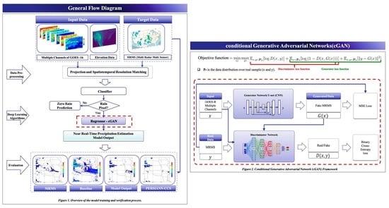Figure 1 illustrates an overview of our framework, which consists of three main components: data pre-processing, deep learning algorithms and evaluation.

Data pre-processing is an essential part of our framework as measurements collected from different spectral bands have different value ranges. For example, 0.86 $\mathsf{\mu }$m (“reflective”) band contains measurements ranging from 0 to 1 while 8.4 $\mathsf{\mu }$m (“cloud-top phase”) band contains measurements ranging from 181 to 323. Normalizing the input is common practice in machine learning as models tend to be biased towards data with the largest value ranges. We make the assumption that all remotely sensed measurements are equally important, so we normalize the data of each channel to range from 0 to 1. Observations of each channel are normalized using the parameters as shown in

Table 1. Parameters for channel normalization applied using the formula: $\frac{value-\min }{\max -\min }$.

Band Number-Wavelength ($\mathsf{\mu }\mathbf{m}$)	$\mathbf{min}$	$\mathbf{max}$
8–6.2	187	260
9–6.9	181	270
10–7.3	171	277
11–8.4	181	323
13–10.3	181	330
14–11.2	172	330

, by subtracting the min value from the channel value and dividing by the difference between the min and max values. Moreover, all the datasets are matched in terms of spatiotemporal resolution to qualify for image-to-image translation. As a result, both the MRMS and imageries from GOES-16 were up-scaled to match the PERSIANN-CCS as the baseline with 30 min temporal and 4 km by 4 km spatial resolution.

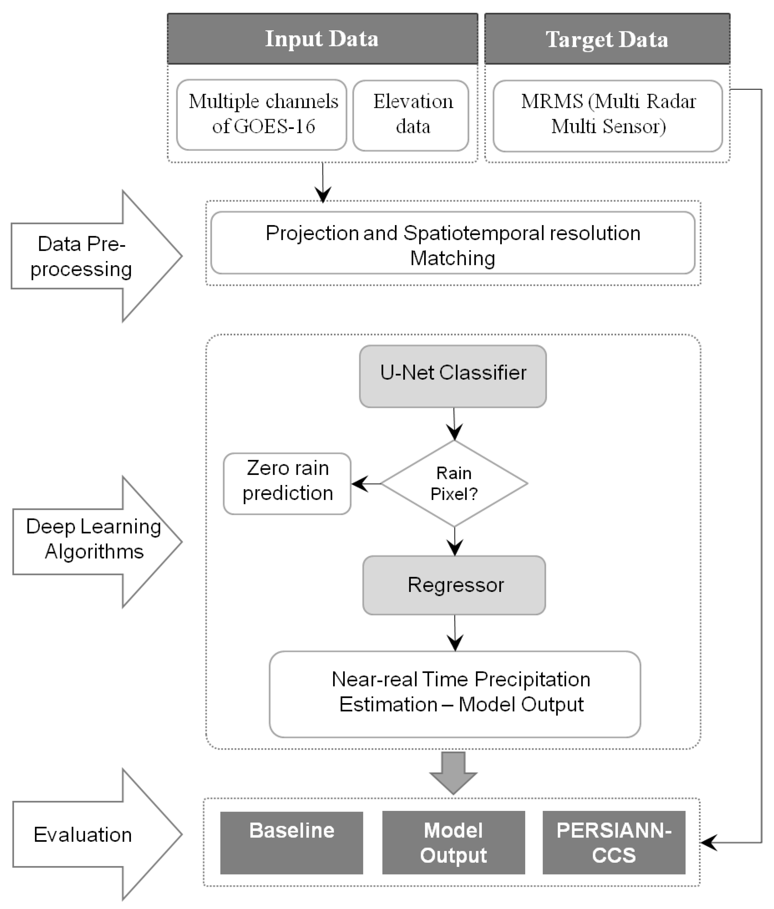
The pre-processed data is then used as input for deep learning algorithms. In this paper, we explore the application of CNNs to learn the relation between input satellite imagery and target precipitation observations. Specifically, we use the U-net architecture that has become popular in recent years in the computer vision—with applications ranging from image-to-image translation to biomedical image segmentation. An illustration of the U-net architecture is presented in Figure 2, which shows an encoder-decoder network but with additional “skip” connections between the encoder and decoder. The bottle-necking of information in the encoder helps capture global spatial information, however, local spatial information is lost in the process. The idea behind the U-net architecture is that decoder accuracy can be improved by passing the lost local spatial information through the skip connections. Accurately capturing local information is important for precipitation estimation as rainfall is generally quite sparse—making pixel-level accuracy that much more important. For more information regarding U-nets please refer to Ronneberger et al. [43].

U-net is used to extract features from the pre-processed input data, which are then used to predict the quantity of rainfall and the classification of rain/no-rain for each pixel. Each extracted feature is the same height and width as the input and target data, and is a single channel; the number of channels was selected through separate cross-validation experiments not discussed in this paper. The single channel feature is then fed into a shallow regression network that predicts a quantity of rain for each pixel. The specific details of each network are shown in

Table 2. Details of network architectures. Each layer of the encoder feeds sequentially into the next layer, from top to bottom (i.e., “conv1” top, so the output of the ”conv7” layer feeds into the “convt1” layer. Additionally, “convt2” and “conv8” layers take not only as input the output from their previous decoder layers but also concatenates the output of the encoder layer of the same row (skip connection). This means the input of the “convt2” layer is the concatenated outputs of the “conv5” and “convt1” layers. The output of the “conv8” layer is the input for the classifier and regressor.

Feature Extractor
Encoder				Decoder
layer	Kernel Size, Stride, Padding	Activation	Batch Norm	layer	Kernel Size, Stride, Padding	Activation	Batch Norm
conv1	$3\times 3\times C\times 64$, 1, 1	ReLU	Yes
conv2	$3\times 3\times 64\times 64$, 1, 1	ReLU	Yes	conv8	$5\times 5\times 65\times 1$, 1, 2	None	No
conv3	$3\times 3\times 64\times 64$, 2, 0	ReLU	Yes
conv4	$3\times 3\times 64\times 128$, 1, 1	ReLU	Yes
conv5	$3\times 3\times 128\times 128$, 1, 1	ReLU	Yes	convt2	$3\times 3\times 129\times 1$, 2, 0	None	No
conv6	$3\times 3\times 128\times 128$, 2, 0	ReLU	Yes
conv7	$3\times 3\times 128\times 128$, 1, 1	ReLU	Yes	convt1	$3\times 3\times 128\times 1$, 2, 0	None	No
Classifier				Regressor
Layer	Kernel Size, Stride, Padding	Activation	Batch Norm	Layer	Kernel Size, Stride, Padding	Activation	Batch Norm
conv1	$3\times 3\times 1\times 1$, 1, 1	Sigmoid	No	conv1	$3\times 3\times 1\times 1$, 1, 1	ReLU	No

C = number of input channels.

.

Performance verification measurements for precipitation amount estimation and rain/no-rain (R/NR) classification are presented in

Table 3. Description of the verification metrics. TP denotes the number of true positive events, MS denotes the number of missing events, FP denotes the number of false-positive events, TN denotes the number of true-negative events.

Verification Measures	Formulas	Range and Desirable Value
Probability of Detection	$\mathrm{POD}=\frac{\mathrm{TP}}{(\mathrm{TP}+\mathrm{MS})}$	Range: 0 to 1; desirable value: 1
False Alarm Ratio	$\mathrm{FAR}=\frac{\mathrm{FP}}{(\mathrm{TP}+\mathrm{FP})}$	Range: 0 to 1; desirable value: 0
Critical Success Index	$\mathrm{CSI}=\frac{\mathrm{TP}}{(\mathrm{TP}+\mathrm{FP}+\mathrm{MS})}$	Range: 0 to 1; desirable value: 1

and

Table 4. Common verification measures for the satellite-based precipitation estimation products.

Verification Measures	Formulas	Range and Desirable Value
Bias	$\mathrm{Bias}=\overline{x}-\overline{y}$	Range: $-\infty$ to $+\infty$; desired value: 0
Mean Squared Error	$\mathrm{MSE}=\frac{1}{N}\sum {(x_i-y_i)}^2$	Range: 0 to $+\infty$; desired value: 0
Pearson’s Correlation Coefficient	$\mathrm{COR}=\frac{\sum (x_i-\overline{x})(y_i-\overline{y})}{\sqrt{\sum {(x_i-\overline{x})}^2}\sqrt{\sum {(y_i-\overline{y})}^2}}$	Range: $-1$ to $+1$; desired value: 1

respectively.

Two baselines are used to be compared to the output of our framework. The first one is the operational product of PERSIANN-CCS and the other one is a framework with the same structure as the proposed one, except that the loss term is calculated using only MSE. The reason to pick this baseline model is to show the superiority of the application of cGAN term in the objective function to better train the network for the task of precipitation estimation.

First phase of the methodology considers the most common scenario: one channel of IR from GOES-16 satellite is used as input to predict target precipitation estimates. In this phase, the networks in our framework (feature extractor and regressor) are trained using the mean squared error (MSE) loss, optimizing the objective:

$$\underset{G_{reg}}{min}{\mathbb{E}}_{x,y\sim \mathbf{Pr}}\left[\parallel y-G_{reg}{\left(x\right)\parallel }_2^2\right],$$

(1)

where Pr is the data distribution over real sample (x and y), $G_{reg}$ is the feature extractor and regressor, x is the input GOES satellite imagery, and y is the target precipitation observation. According to this phase experiments, the regressor predicts small quantities of rain when the target indicates no-rain pixels. Instead of deciding on an arbitrary threshold to truncate values with, we follow the work of Tao et al. [15] and use a shallow classification network to predict a rain/no-rain label for each pixel—a binary mask. Tao et al. (2018) applied Stacked Denoising Autoencoders (SDAEs) to delineate the rain/no-rain precipitation regions from bispectral satellite information. SDAEs are common and simple DNNs consisting of an autoencoder to extract representative features and learn from input to predict the output. The binary mask in our study is used to update the regression network’s prediction—pixels where the classification network predicts no-rain is updated to zero. The classifier uses the same single channel feature from the feature extractor as the regressor (details of the classifier are shown in Table 2). This gives us an updated objective of:

$$\begin{array}{cc}\hfill & \underset{G_{reg},G_{cls}}{min}{\mathbb{E}}_{x,y\sim \mathbf{Pr}}\left[\parallel y-G_{reg}\left(x\right)·G_{cls}{\left(x\right)\parallel }_2^2\right]+\hfill \\ \hfill & {\mathbb{E}}_{x,\widehat{y}\sim \mathbf{Pr}}\left[\widehat{y}·log\left(G_{cls}\left(x\right)\right)+(1-\widehat{y})·log(1-G_{cls}\left(x\right))\right],\hfill \end{array}$$

(2)

where $G_{cls}$ is the feature extractor and classifier and $\widehat{y}$ is the binarized version of y. Here the feature extractor in $G_{cls}$ share the same weights as those in $G_{reg}$.

As mean squared error (MSE) is a commonly used objective for the task of precipitation estimation, we use it as our optimization objective in the first phase. Using MSE, however, we find the outputs from precipitation estimators to be highly skewed toward smaller values due to the dominance of no-rain pixels, as well as, the rarity of pixels with heavy rain. This means that MSE by itself is insufficient in driving the model to capture the true underlying distribution of precipitation values. And since one of the main purposes of satellite-based precipitation estimation is to specifically track extreme events with negative environmental consequences, this behavior is problematic.

The second phase of our methodology looks to address this problematic behavior. We follow along the same line as Tao et al. [15], who tried to remedy this behavior with the addition of a Kullback-Leibler (KL) divergence term to the optimization objective. KL divergence measures how one probability distribution p diverges from a second expected probability distribution q:

$$D_{KL}(p\parallel q)={\int }_{x}p\left(x\right)log\frac{p\left(x\right)}{q\left(x\right)}dx$$

(3)

$D_{KL}$ achieves the minimum zero when $p\left(x\right)$ and $q\left(x\right)$ are equal everywhere. It is noticeable according to the formula that KL divergence is asymmetric. In cases where $p\left(x\right)$ is close to zero but $q\left(x\right)$ is significantly non-zero, then the effect of q is disregarded. This makes optimizing difficult when using gradient methods as there is no gradient to update parameters in such cases [44].

We consider instead a different measure, the Jensen-Shannon (JS) divergence:

$$D_{JS}(p\parallel q)=\frac{1}{2}{D}_{KL}(p\parallel \frac{p+q}{2})+\frac{1}{2}{D}_{KL}(q\parallel \frac{p+q}{2})$$

(4)

JS divergence is not only symmetric but is a smoother function compared to KL divergence, making it better suited to use with gradient methods. Huszár [45] have demonstrated the superiority of JS divergence over the KL divergence for quantifying the similarity between two probability distributions. An implementation of JS divergence is a generative adversarial network (GAN), which adds a discriminator network that works against a generator network. The discriminator network discriminates whether the given input is a real sample from the true distribution (ground truth) or is a fake sample from a fake distribution (output from the generative network) and the generator network attempts to fool the discriminator. The GAN concept is illustrated in Figure 3, where G is a generator network and D is a discriminator network. For further detail on GANs structure please refer to the papers by Goodfellow et al. [37] and Goodfellow [46].

In our setup, the generator consist of the previously mentioned networks (feature extractor, classifier and regressor) and a fake sample is an output from the regressor that has been updated using the binary mask from the classifier. Updating Equation (2) to include the discriminator network for GAN gives the following equation:

$$\begin{array}{cc}\hfill \underset{G_{reg},G_{cls}}{min}\underset{D}{max}& {\mathbb{E}}_{x,y\sim \mathbf{Pr}}\left[\parallel y-G_{reg}\left(x\right)·G_{cls}{\left(x\right)\parallel }_2^2\right]+\hfill \\ \hfill & {\mathbb{E}}_{x,\widehat{y}\sim \mathbf{Pr}}\left[\widehat{y}·log\left(G_{cls}\left(x\right)\right)+(1-\widehat{y})·log(1-G_{cls}\left(x\right))\right]+\hfill \\ \hfill & {\mathbb{E}}_{x,y\sim \mathbf{Pr}}\left[log\left(D\right(x,y\left)\right)\right]+{\mathbb{E}}_{x\sim \mathbf{Pr}}\left[log(1-D(x,G_{reg}\left(x\right)·G_{cls}\left(x\right)\right],\hfill \end{array}$$

(5)

where D is the discriminator. Unlike the previously discussed discriminator that only looks at the target y or simulated target $G_{reg}·G_{cls}$, here we use a discriminator that also looks at the corresponding input x as reference. This is known as a conditional generative adversarial network (cGAN), as now the discrimination of the true or fake distribution is conditioned on the input x. cGANs have been shown to perform even better than GANs but requires paired $x,y$ data, which is not always readily available Mirza and Osindero [47]. However, in this study, the paired data is provided by spatiotemporal resolution matching of the inputs (GOES-R bands) and the observation data (MRMS). Our setup follows closely to that of Isola et al. [48] as we consider pixel-wise precipitation estimation from satellite imagery as the image-to-image translation problem from computer vision. The notable differences between our setup and that of Isola et al. [48] are the generator network structure and objective function. While the objective function of Isola et al. [48] contains only two parts: L1 on the generator and binary cross-entropy on the discriminator, our final objective function (Equation (5)) contains three parts: L2 on the generator, binary cross-entropy on the discriminator and binary cross-entropy on the output of the classifier. The optimal point for the min-max equation is known from game theory, which is when the discriminator and the generator reach a Nash equilibrium. That’s the point when the discriminator is not able to tell the difference between the fake samples and the ground truth data anymore.

The last phase of the methodology considers the infusion of other channels of GOES-16 satellite data and GTOPO30 elevation information as an ancillary data. We first evaluate selected channels of GOES-16 individually with and without inclusion of elevation data to establish a baseline for how informative each individual channel is for precipitation estimation. We then evaluate combinations of GOES-16 channels to see how well different channels complement each other.

4. Results

In this section, we evaluate the performance of the proposed algorithm over the verification period for the continental United States. We compare the operational product PERSIANN-CCS, in addition to a baseline model that is trained using conventional and commonly used metric MSE as its objective function. The MRMS data is used as the ground truth data to investigate the performance improvement in both detecting the rain/no-rain pixels and the estimates.

Table 5. Statistical evaluation metrics values for different scenarios using single spectral bands

Sc.	Band Number/Wavelength ($\mathsf{\mu }$m)	MSE (mm h${}^{-1}$ )${}^2$	COR	BIAS	POD	FAR	CSI	MSE	COR	BIAS	POD	FAR	CSI
cGAN Model Output
		Without Elevation						With Elevation
1	8–6.2	1.410	0.270	−0.030	0.356	0.734	0.174	1.096	0.311	−0.017	0.363	0.726	0.180
2	9–6.9	1.452	0.271	−0.044	0.371	0.725	0.182	1.107	0.317	−0.032	0.428	0.736	0.190
3	10–7.3	1.536	0.281	−0.090	0.474	0.755	0.188	1.105	0.313	−0.037	0.450	0.727	0.200
4	11–8.4	1.310	0.271	−0.034	0.507	0.714	0.219	1.053	0.326	−0.047	0.599	0.726	0.229
5	13–10.3	1.351	0.262	−0.041	0.518	0.718	0.220	1.037	0.323	−0.039	0.594	0.731	0.224
PERSIANN-CCS
		MSE		COR		BIAS		POD		FAR		CSI
	10.8 $\mathsf{\mu }$m	2.174		0.220		−0.046		0.284		0.622		0.193

provides the overall statistic performances of the cGAN model compared to PERSIANN-CCS with reference to the MRMS data. Multiple channels are considered stand-alone and as the input to the proposed model including channel 13 with similar wavelength to PERSIANN-CCS to make the comparison fair.

The elevation data is also considered as another input to the model along with single bands of ABI GOES-16 to investigate the effect of infusing elevation data as auxiliary information. All evaluation metrics show improved results for the proposed cGAN model over the operational PERSIANN-CCS product during the verification period using band number 13. Specifically, the application of elevation data combined with single spectral bands indicates further performance improvement. Beside channel 13 as input to the model, utilization of channel 11 (“Cloud Top Phase”) as a stand-alone input to the model also shows good performance due to the statistics from evaluation metrics. It could be concluded that channel 11 is also playing an important role as channel 13 in providing useful information for the task of precipitation estimation either utilized as stand-alone or combined with elevation information.

Multiple scenarios are considered as shown in

Table 6. Statistical evaluation metrics values for different scenarios using multiple spectral bands.

Sc.	Band Number/Wavelength ($\mathsf{\mu }$m)	MSE (mm h${}^{-1}$)${}^2$	COR	BIAS	POD	FAR	CSI
cGAN Model Output
1	8,11–6.2, 8.4	1.349	0.353	−0.094	0.635	0.683	0.266
2	9,11–6.9, 8.4	1.317	0.345	−0.088	0.627	0.667	0.275
3	10,11–7.3, 8.4	1.385	0.343	−0.119	0.668	0.681	0.274
4	8,9,10,11–6.2, 6.9, 7.3, 8.4	1.170	0.319	−0.064	0.601	0.658	0.275
5	8,13–6.2, 10.3	1.350	0.348	−0.100	0.644	0.689	0.264
6	9,13–6.9, 10.3	1.410	0.344	−0.124	0.661	0.678	0.275
7	10,13–7.3, 8.4	1.408	0.337	−0.129	0.665	0.676	0.277
8	8,9,10,13–6.2, 6.9, 7.3, 10.3	1.258	0.317	−0.077	0.594	0.655	0.274
9	8,9,10,11,12,13,14–6.2, 6.9, 7.3, 8.4, 9.6, 10.3, 11.2	1.178	0.359	−0.086	0.706	0.681	0.278
PERSIANN-CCS
		MSE (mm h${}^{-1}$)${}^2$	COR	BIAS	POD	FAR	CSI
	10.8 $\mathsf{\mu }$m	2.174	0.220	−0.046	0.284	0.622	0.193

to investigate the benefit that channels 11 and 13 provide for the model in combination with some other spectral bands including different levels of water vapor. The evaluation metrics values indicate that the utilization of more spectral bands as input to the proposed model (Sc. 9), leads to lower MSE and higher correlation and CSI.

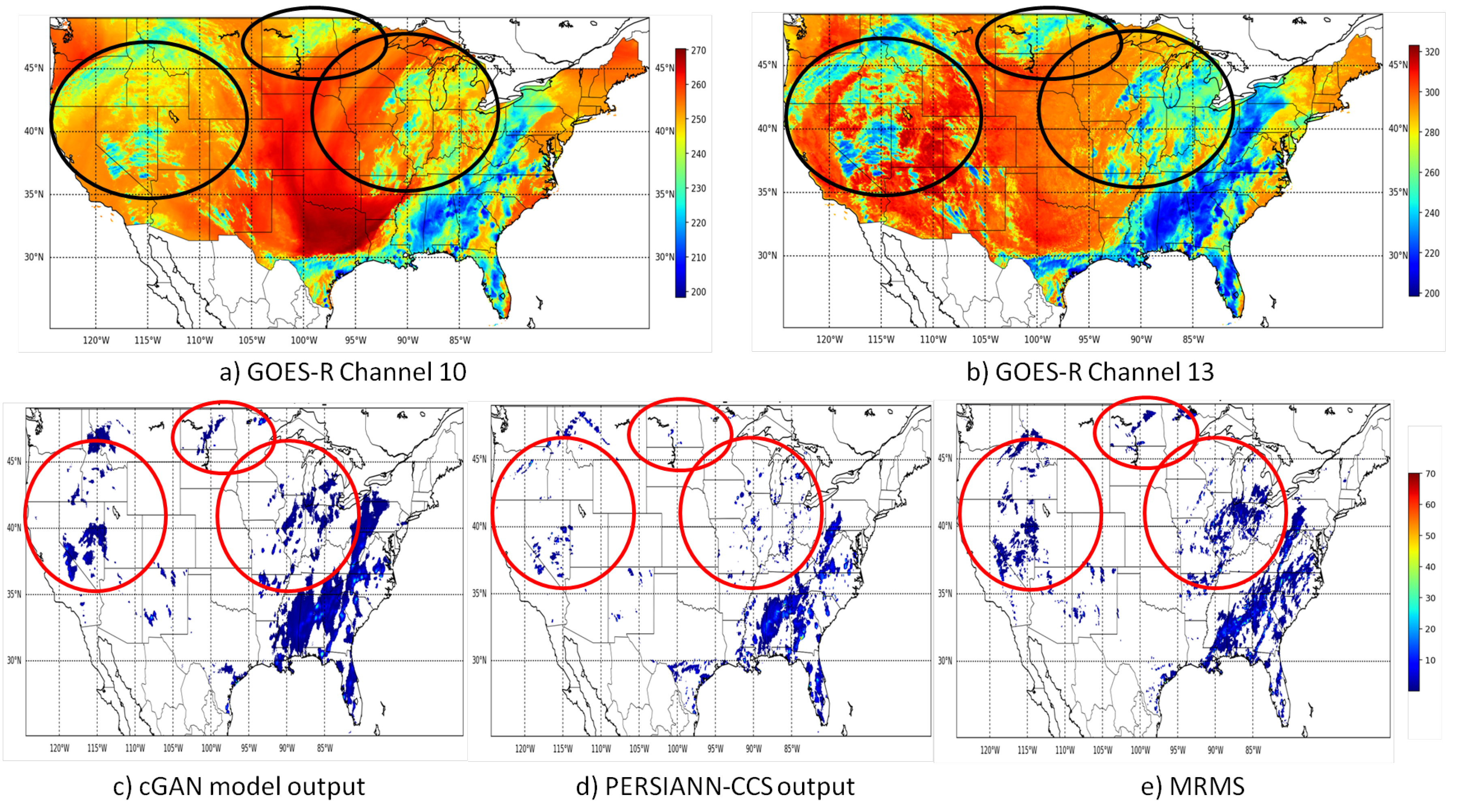
Visualization of predicted precipitation values for the proposed cGAN model and operational PERSIANN-CCS product are shown in Figure 4 to emphasize the performance improvement specifically over the regions covered with warm clouds. Capturing clouds with higher temperature associated with rainfall is an important issue that is considered as the main drawback for precipitation retrieval algorithms such as PERSIANN-CCS. This inherent shortcoming is associated with the temperature threshold based segmentation part of the algorithm incapable of fully extracting warm raining clouds [9]. Figure 4 is showing two sample IR band types and the half-hourly precipitation maps from the proposed model using the inputs listed in the scenario number 9 in Table 6 for 31 July at 22:00—UTC along with the PERSIANN-CCS output and MRMS data for the same time step.

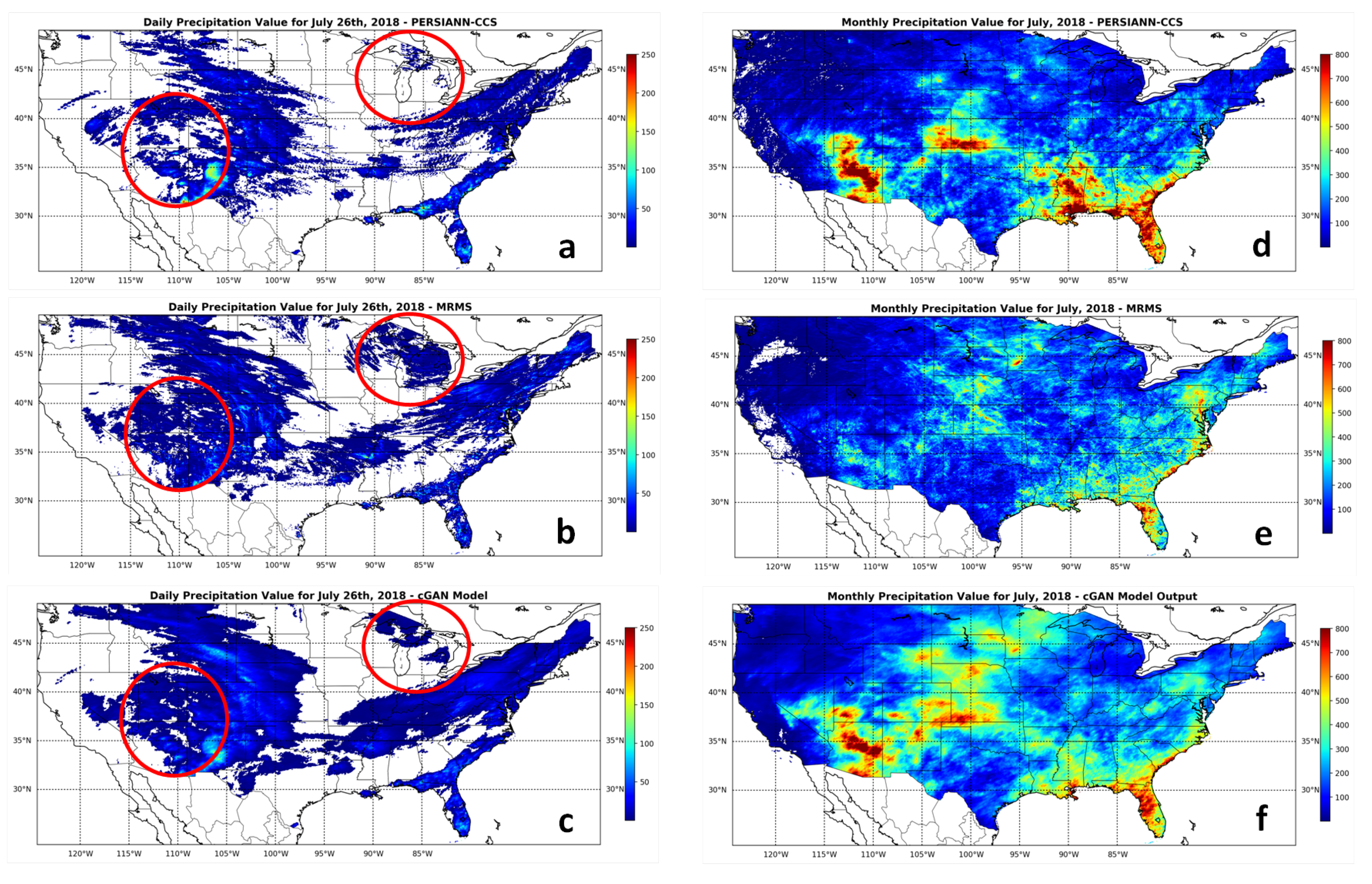
Daily and monthly values for all the models are also provided in Figure 5. As shown in the red circled regions for the precipitation values with daily scale in the left panel, the proposed cGAN model output is capturing more of the precipitation as compared to PERSIANN-CCS output. Although both models are showing overestimation compared to MRMS in monthly scale, precipitation values from the proposed model are closer to the ground truth extreme values than PERSIANN-CCS.

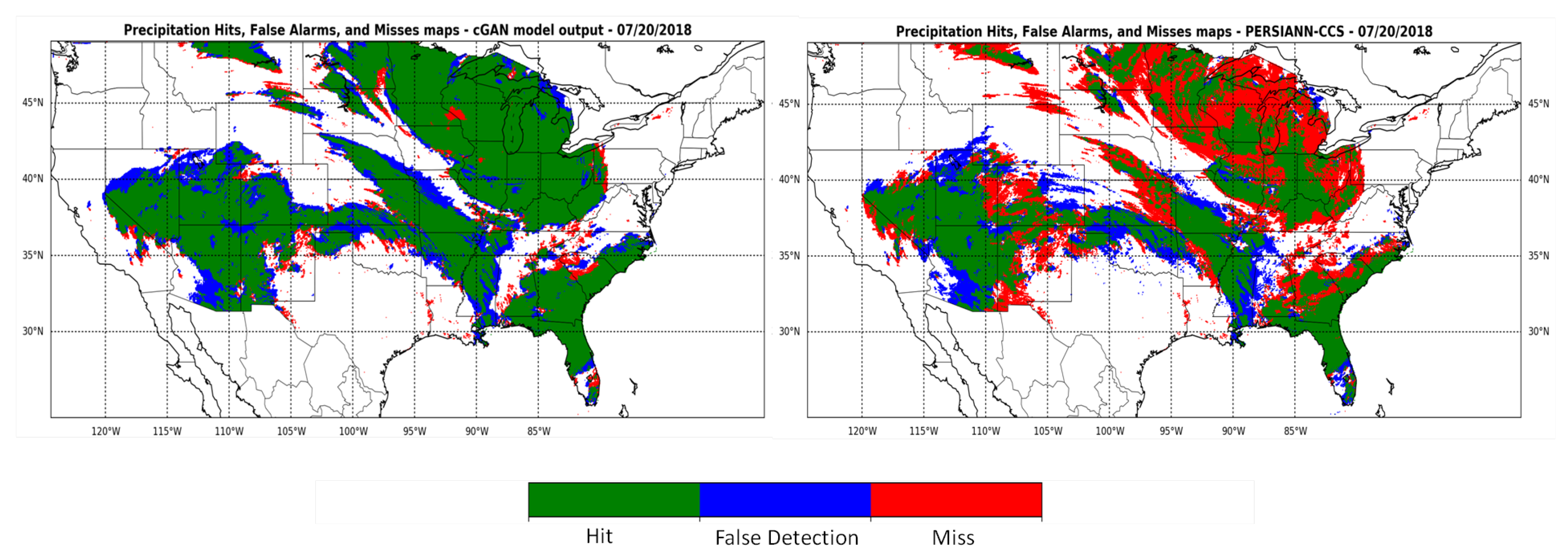
Figure 6 presents R/NR identification results for the proposed cGAN model and the PERSIANN-CCS models for the 20th of July 2018. It is obvious that only small sections of rainfall are correctly identified by PERSIANN-CCS while cGAN model is able to reduce the missing rainy pixels and shows a significant improvement in delineating the precipitation area, represented by green pixels. More pixels with false detection of rainfall are observed in cGAN model output than PERSIANN-CCS which are insignificant compared to much higher detection and lower miss of rainy pixels.

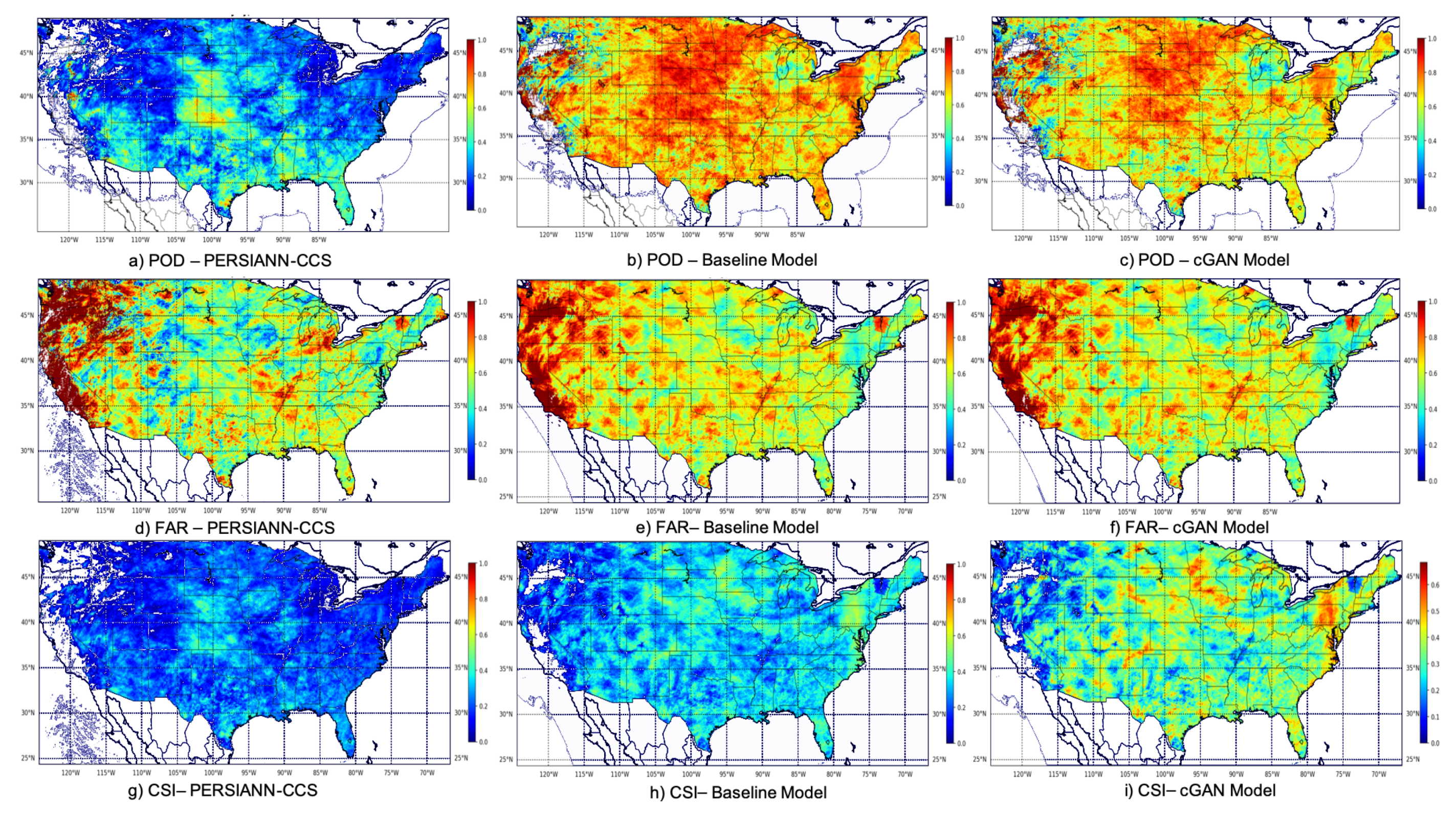
Figure 7 presents the maps of POD, FAR and CSI values for the cGAN model compared to PERSIANN-CCS and the baseline model with MSE as the loss function. As explained in the methodology section, the cGAN model’s loss term consists of an additional part other than MSE that has to be optimized as a min-max problem in order to better capture complex precipitation distribution. Figure 7 indicates the common verification measurements in Table 3 for regression performance of all three models during the verification period. High measurement values are represented by warm colors and low measurement values are indicated by cold colors. Note that high values are desirable for POD and CSI, while lower values are desirable for FAR. Figure 7 shows that the cGAN model outperforms the PERSIANN-CCS almost all over the CONUS and is showing better performance over the baseline model as well. For FAR, higher values observed for cGAN model are negligible considering the significant improvement of POD over the baseline model and PERSIANN-CCS. An ascending order can be observed in the maps of CSI of PERSIANN-CCS, the baseline model and the cGAN model.

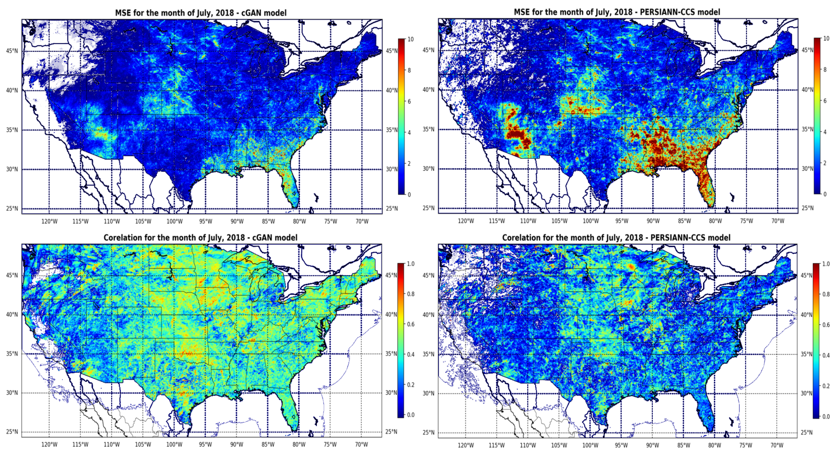
Correlation and MSE values are also visualized to help to better explain the performance improvement of the cGAN model over PERSIANN-CCS over the verification period in Figure 8.

5. Conclusions

This paper takes advantage of advanced deep learning techniques, to investigate their capability of effectively and automatically learning the relation between multiple sources of inputs and observation. A two-stage framework using a more complex objective function for training a CNN from multiple channels of latest generation of geostationary satellites is introduced to better capture the complex properties of precipitation. The effectiveness of the proposed model is investigated by comparing it with an operational satellite-based precipitation product (PERSIANN-CCS) and a baseline model with a conventional type of objective function. The first stage is based on a classification model to delineate precipitation regions and the second stage is a precipitation amount estimation model. The model is calibrated and evaluated over the continental United States.

The evaluation metrics are compared for different scenarios defined to investigate the benefit that each channel provides for the model individually or in combination with other spectral bands. The experimental results demonstrated the general effectiveness of the cGAN two-stage deep learning framework over the PERSIANN-CCS and the baseline model. The proposed model shows the best performance with the application of most of the emissive channels from GOES-16, listed in scenario 9 in Table 6 over the verification period which is July 2018 in this study.

The overall performance is improved compared to the baseline model and operational product of PERSIANN-CCS even with the application of IR channel solely as the input of cGAN model to make the comparison fair. The model is capable of capturing the relationship between the satellite information and the precipitation even at locations covered with warm clouds, which is an important drawback associated with satellite-based precipitation estimation products with global coverage. Moreover, the application of elevation data combined with low number of spectral bands used as input showed performance improvement. We conclude that the model’s performance will be improved using the elevation data as an ancillary information to each channel of the satellite and helps the precipitation estimation task to be more accurate and generalized on a larger scale.

The current investigation is a preliminary step as a proof of concept for global application and toward supporting NASA’s GPM mission to develop effective multi-satellite precipitation retrieval algorithms for the fusion of precipitation information from multi-satellite platforms. Future works include organizing a data-driven software package capable of exploiting NASA data sets, usable in different study regions and for other geoscience applications. Further experiments are required for the preparation of the model to serve as an operational product.

References

1. Sorooshian, S.; AghaKouchak, A.; Arkin, P.; Eylander, J.; Foufoula-Georgiou, E.; Harmon, R.; Hendrickx, J.M.; Imam, B.; Kuligowski, R.; Skahill, B.; et al. Advanced concepts on remote sensing of precipitation at multiple scales. Bull. Am. Meteorol. Soc. 2011, 92, 1353–1357. [Google Scholar] [CrossRef]
2. Nguyen, P.; Shearer, E.J.; Tran, H.; Ombadi, M.; Hayatbini, N.; Palacios, T.; Huynh, P.; Braithwaite, D.; Updegraff, G.; Hsu, K.; et al. The CHRS Data Portal, an easily accessible public repository for PERSIANN global satellite precipitation data. Sci. Data 2019, 6, 180296. [Google Scholar] [CrossRef] [PubMed] [Green Version]
3. Ba, M.B.; Gruber, A. GOES multispectral rainfall algorithm (GMSRA). J. Appl. Meteorol. 2001, 40, 1500–1514. [Google Scholar] [CrossRef]
4. Behrangi, A.; Imam, B.; Hsu, K.; Sorooshian, S.; Bellerby, T.J.; Huffman, G.J. REFAME: Rain estimation using forward-adjusted advection of microwave estimates. J. Hydrometeorol. 2010, 11, 1305–1321. [Google Scholar] [CrossRef]
5. Behrangi, A.; Hsu, K.l.; Imam, B.; Sorooshian, S.; Huffman, G.J.; Kuligowski, R.J. PERSIANN-MSA: A precipitation estimation method from satellite-based multispectral analysis. J. Hydrometeorol. 2009, 10, 1414–1429. [Google Scholar] [CrossRef]
6. Behrangi, A.; Hsu, K.l.; Imam, B.; Sorooshian, S.; Kuligowski, R.J. Evaluating the utility of multispectral information in delineating the areal extent of precipitation. J. Hydrometeorol. 2009, 10, 684–700. [Google Scholar] [CrossRef]
7. Martin, D.W.; Kohrs, R.A.; Mosher, F.R.; Medaglia, C.M.; Adamo, C. Over-ocean validation of the global convective diagnostic. J. Appl. Meteorol. Climatol. 2008, 47, 525–543. [Google Scholar] [CrossRef]
8. Tao, Y.; Gao, X.; Ihler, A.; Hsu, K.; Sorooshian, S. Deep neural networks for precipitation estimation from remotely sensed information. In Proceedings of the 2016 IEEE Congress on Evolutionary Computation (CEC), Vancouver, BC, Canada, 24–29 July 2016; pp. 1349–1355. [Google Scholar]
9. Hayatbini, N.; Hsu, K.L.; Sorooshian, S.; Zhang, Y.; Zhang, F. Effective Cloud Detection and Segmentation Using a Gradient-Based Algorithm for Satellite Imagery: Application to Improve PERSIANN-CCS. J. Hydrometeorol. 2019, 20, 901–913. [Google Scholar] [CrossRef] [Green Version]
10. Joyce, R.J.; Janowiak, J.E.; Arkin, P.A.; Xie, P. CMORPH: A method that produces global precipitation estimates from passive microwave and infrared data at high spatial and temporal resolution. J. Hydrometeorol. 2004, 5, 487–503. [Google Scholar] [CrossRef]
11. Kidd, C.; Kniveton, D.R.; Todd, M.C.; Bellerby, T.J. Satellite rainfall estimation using combined passive microwave and infrared algorithms. J. Hydrometeorol. 2003, 4, 1088–1104. [Google Scholar] [CrossRef]
12. Huffman, G.J.; Bolvin, D.T.; Braithwaite, D.; Hsu, K.; Joyce, R.; Xie, P.; Yoo, S.H. NASA global precipitation measurement (GPM) integrated multi-satellite retrievals for GPM (IMERG). Algorithm Theor. Basis Doc. Version 2015, 4, 30. [Google Scholar]
13. Huffman, G.J.; Bolvin, D.T.; Nelkin, E.J.; Wolff, D.B.; Adler, R.F.; Gu, G.; Hong, Y.; Bowman, K.P.; Stocker, E.F. The TRMM multisatellite precipitation analysis (TMPA): Quasi-global, multiyear, combined-sensor precipitation estimates at fine scales. J. Hydrometeorol. 2007, 8, 38–55. [Google Scholar] [CrossRef]
14. Hong, Y.; Hsu, K.L.; Sorooshian, S.; Gao, X. Precipitation estimation from remotely sensed imagery using an artificial neural network cloud classification system. J. Appl. Meteorol. 2004, 43, 1834–1853. [Google Scholar] [CrossRef]
15. Tao, Y.; Hsu, K.; Ihler, A.; Gao, X.; Sorooshian, S. A two-stage deep neural network framework for precipitation estimation from Bispectral satellite information. J. Hydrometeorol. 2018, 19, 393–408. [Google Scholar] [CrossRef]
16. Bengio, Y. Learning deep architectures for AI. Found. Trends Mach. Learn. 2009, 2, 1–127. [Google Scholar] [CrossRef]
17. Hinton, G.E. Deep belief networks. Scholarpedia 2009, 4, 5947. [Google Scholar] [CrossRef]
18. LeCun, Y.; Bengio, Y.; Hinton, G. Deep learning. Nature 2015, 521, 436. [Google Scholar] [CrossRef] [PubMed]
19. Liu, Z.; Zhou, P.; Chen, X.; Guan, Y. A multivariate conditional model for streamflow prediction and spatial precipitation refinement. J. Geophys. Res. Atmos. 2015, 120. [Google Scholar] [CrossRef]
20. Rasp, S.; Pritchard, M.S.; Gentine, P. Deep learning to represent subgrid processes in climate models. Proc. Natl. Acad. Sci. USA 2018, 115, 9684–9689. [Google Scholar] [CrossRef] [Green Version]
21. Reichstein, M.; Camps-Valls, G.; Stevens, B.; Jung, M.; Denzler, J.; Carvalhais, N.; Prabhat. Deep learning and process understanding for data-driven Earth system science. Nature 2019, 566, 195. [Google Scholar] [CrossRef]
22. Akbari Asanjan, A.; Yang, T.; Hsu, K.; Sorooshian, S.; Lin, J.; Peng, Q. Short-Term Precipitation Forecast Based on the PERSIANN System and LSTM Recurrent Neural Networks. J. Geophys. Res. Atmos. 2018, 123, 12–543. [Google Scholar] [CrossRef]
23. Pan, B.; Hsu, K.; AghaKouchak, A.; Sorooshian, S. Improving Precipitation Estimation Using Convolutional Neural Network. Water Resour. Res. 2019, 55, 2301–2321. [Google Scholar] [CrossRef] [Green Version]
24. Goodfellow, I.; Bengio, Y.; Courville, A. Deep Learning; MIT Press: Cambridge, MA, USA, 2016; Available online: http://www.deeplearningbook.org (accessed on 20 September 2019).
25. Schmidhuber, J. Deep learning in neural networks: An overview. Neural Netw. 2015, 61, 85–117. [Google Scholar] [CrossRef] [PubMed] [Green Version]
26. Shen, D.; Wu, G.; Suk, H.I. Deep learning in medical image analysis. Annu. Rev. Biomed. Eng. 2017, 19, 221–248. [Google Scholar] [CrossRef] [PubMed]
27. Vandal, T.; Kodra, E.; Ganguly, A.R. Intercomparison of machine learning methods for statistical downscaling: The case of daily and extreme precipitation. Theor. Appl. Climatol. 2019, 137, 557–570. [Google Scholar] [CrossRef]
28. Tao, Y.; Gao, X.; Ihler, A.; Sorooshian, S.; Hsu, K. Precipitation identification with bispectral satellite information using deep learning approaches. J. Hydrometeorol. 2017, 18, 1271–1283. [Google Scholar] [CrossRef]
29. Liu, Y.; Racah, E.; Prabhat; Correa, J.; Khosrowshahi, A.; Lavers, D.; Kunkel, K.; Wehner, M.; Collins, W. Application of deep convolutional neural networks for detecting extreme weather in climate datasets. arXiv 2016, arXiv:1605.01156. [Google Scholar]
30. Xingjian, S.; Chen, Z.; Wang, H.; Yeung, D.Y.; Wong, W.K.; Woo, W.C. Convolutional LSTM network: A machine learning approach for precipitation nowcasting. In Advances in Neural Information Processing Systems; The MIT Press: Cambridge, MA, USA, 2015; pp. 802–810. [Google Scholar]
31. LeCun, Y.; Boser, B.; Denker, J.S.; Henderson, D.; Howard, R.E.; Hubbard, W.; Jackel, L.D. Backpropagation applied to handwritten zip code recognition. Neural Comput. 1989, 1, 541–551. [Google Scholar] [CrossRef]
32. Elman, J.L. Finding structure in time. Cogn. Sci. 1990, 14, 179–211. [Google Scholar] [CrossRef]
33. Jordan, M.I. Serial order: A parallel distributed processing approach. In Advances in Psychology; Elsevier: Amsterdam, The Netherlands, 1997; Volume 121, pp. 471–495. [Google Scholar]
34. Krizhevsky, A.; Sutskever, I.; Hinton, G.E. Imagenet classification with deep convolutional neural networks. In Advances in Neural Information Processing Systems; The MIT Press: Cambridge, MA, USA, 2012; pp. 1097–1105. [Google Scholar]
35. Vincent, P.; Larochelle, H.; Bengio, Y.; Manzagol, P.A. Extracting and composing robust features with denoising autoencoders. In Proceedings of the 25th International Conference on Machine Learning, Helsinki, Finland, 5–9 July 2008; ACM: New York, NY, USA, 2008; pp. 1096–1103. [Google Scholar] [Green Version]
36. Pu, Y.; Gan, Z.; Henao, R.; Yuan, X.; Li, C.; Stevens, A.; Carin, L. Variational autoencoder for deep learning of images, labels and captions. In Advances in Neural Information Processing Systems; The MIT Press: Cambridge, MA, USA, 2016; pp. 2352–2360. [Google Scholar]
37. Goodfellow, I.; Pouget-Abadie, J.; Mirza, M.; Xu, B.; Warde-Farley, D.; Ozair, S.; Courville, A.; Bengio, Y. Generative adversarial nets. Advances in Neural Information Processing Systems; The MIT Press: Cambridge, MA, USA, 2014; pp. 2672–2680. [Google Scholar]
38. Schmit, T.J.; Gunshor, M.M.; Menzel, W.P.; Gurka, J.J.; Li, J.; Bachmeier, A.S. Introducing the next-generation Advanced Baseline Imager on GOES-R. Bull. Am. Meteorol. Soc. 2005, 86, 1079–1096. [Google Scholar] [CrossRef]
39. NOAA’s Comprehensive Large Array-data Stewardship System. Available online: https://www.avl.class.noaa.gov/saa/products/welcome/ (accessed on 1 October 2018).
40. Schmit, T.J.; Menzel, W.P.; Gurka, J.; Gunshor, M. The ABI on GOES-R. In Proceedings of the 6th Annual Symposium on Future National Operational Environmental Satellite Systems-NPOESS and GOES-R, Atlanta, GA, USA, 16–21 January 2010. [Google Scholar]
41. GPM Ground Validation Data Archieve. Available online: https://gpm-gv.gsfc.nasa.gov/ (accessed on 1 November 2018).
42. Danielson, J.J.; Gesch, D.B. Global Multi-Resolution Terrain Elevation Data 2010 (GMTED2010), Technical report; US Geological Survey: Reston, VA, USA, 2011. [Google Scholar]
43. Ronneberger, O.; Fischer, P.; Brox, T. U-net: Convolutional networks for biomedical image segmentation. In Proceedings of the International Conference on Medical Image Computing and Computer-Assisted Intervention, Munich, Germany, 5–9 October 2015; Springer: Berlin, Germany, 2015; pp. 234–241. [Google Scholar]
44. Arjovsky, M.; Chintala, S.; Bottou, L. Wasserstein gan. arXiv 2017, arXiv:1701.07875. [Google Scholar]
45. Huszár, F. How (not) to train your generative model: Scheduled sampling, likelihood, adversary? arXiv 2015, arXiv:1511.05101. [Google Scholar]
46. Goodfellow, I. NIPS 2016 tutorial: Generative adversarial networks. arXiv 2016, arXiv:1701.00160. [Google Scholar]
47. Mirza, M.; Osindero, S. Conditional generative adversarial nets. arXiv 2014, arXiv:1411.1784. [Google Scholar]
48. Isola, P.; Zhu, J.Y.; Zhou, T.; Efros, A.A. Image-to-image translation with conditional adversarial networks. In Proceedings of the IEEE Conference on Computer Vision and Pattern Recognition, Honolulu, HI, USA, 21–26 July 2017; pp. 1125–1134. [Google Scholar]
Figure 1. The proposed framework for the Precipitation Estimation.
Remotesensing 11 02193 g001
Figure 2. Visualized structure of U-net network.
Remotesensing 11 02193 g002
Figure 3. Schematic conditional Generative Adversarial Network Structure.
Remotesensing 11 02193 g003
Figure 4. (a) Channels 10 and (b) 13 from ABI GOES-16 imagery; (c) cGAN model half hourly output; (d) PERSIANN-CCS half hourly precipitation values; and (e) The MRMS data for 31 July 2018 at 22:00 UTC over the CONUS.Black circles on GOES-16 satellite imagery represent regions with warm clouds and the red circles are the corresponding regions with the rainfall associated with the warm clouds.
Remotesensing 11 02193 g004
Figure 5. Daily (left panel) and monthly (right panel) precipitation values for (a,d) PERSIANN-CCS; (c,f) cGAN model output compared to the (b,e) Reference data—MRMS. Red circles are highlighting regions with most of the differences.
Remotesensing 11 02193 g005
Figure 6. Visualization of precipitation identification performance of PERSIANN-CCS vs cGAN model output over the United States for 20 July 2018.
Remotesensing 11 02193 g006
Figure 7. POD (top row), FAR (middle row) and CSI (bottom row) of PERSIANN-CCS (left column), the baseline model (middle column) and the cGAN model (right column) over the United States for July 2018.
Remotesensing 11 02193 g007
Figure 8. The Correlation and mean square error (MSE) values (mm h 1 ) 2 for the cGAN and PERSIANN-CCS model over the CONUS and during the validation period (month of July 2018).
Remotesensing 11 02193 g008