A Scheme for the Long-Term Monitoring of Impervious−Relevant Land Disturbances Using High Frequency Landsat Archives and the Google Earth Engine


Abstract
:1. Introduction
- Classification performance is dependent on advanced classification algorithms. Over the past decades, supervised classifiers have especially grown in utility to accommodate complex feature [24,25], such as Random Forests (RF) [26]. These classifiers have been widely used for annual classification to generate time series maps of the informed land covers, in order to determine both the states and trends of the changes [6,11,14,24,27,28,29]. However, sensitivity to training data is a common issue for most supervised classifiers [24,25]. On the other hand, post-classification approaches are indispensable for improving spatial-temporal consistency of the classification results [11,28,29].
- Thresholding-based extraction has been widely employed in identifying specific land covers in the time series [23]. Significant deviations between the target and other land covers are the key to detecting the target. Thus, images need to be transformed into the dimension that is sensitive to the target [21,23], such as the NUACI (Normalized Urban Areas Composite Index) [21], which was proposed for the multi-temporal mapping of global urban lands. Thresholding-based extraction is indeed convenient but highly dependent on the predefined threshold [23].
- Spectral trajectory-based detection is a milestone in monitoring changes with Landsat time series [15,19,23]. Detection approaches using high temporal frequency satellite data have become a frontier of research, enabling a more nuanced understanding of changes on the Earth [15,19], for instance, the vegetation change tracker (VCT) [30], Landsat-based detection of Trends in Disturbance and Recovery (LandTrendr) [31], an algorithm based on statistical quality control charts [32], Continuous Change Detection and Classification (CCDC) [33], Continuous Subpixel Monitoring (CSM) [10], and Continuous monitoring of Land Disturbance (COLD) [34]. These spectral trajectory-based methods are well adopted in diverse thematic domains. However, implementing these methods often requires rigorous data pre-processing, affordable computation, and time-consuming operations, which limits their more extensive applications.
2. Study Area and Data
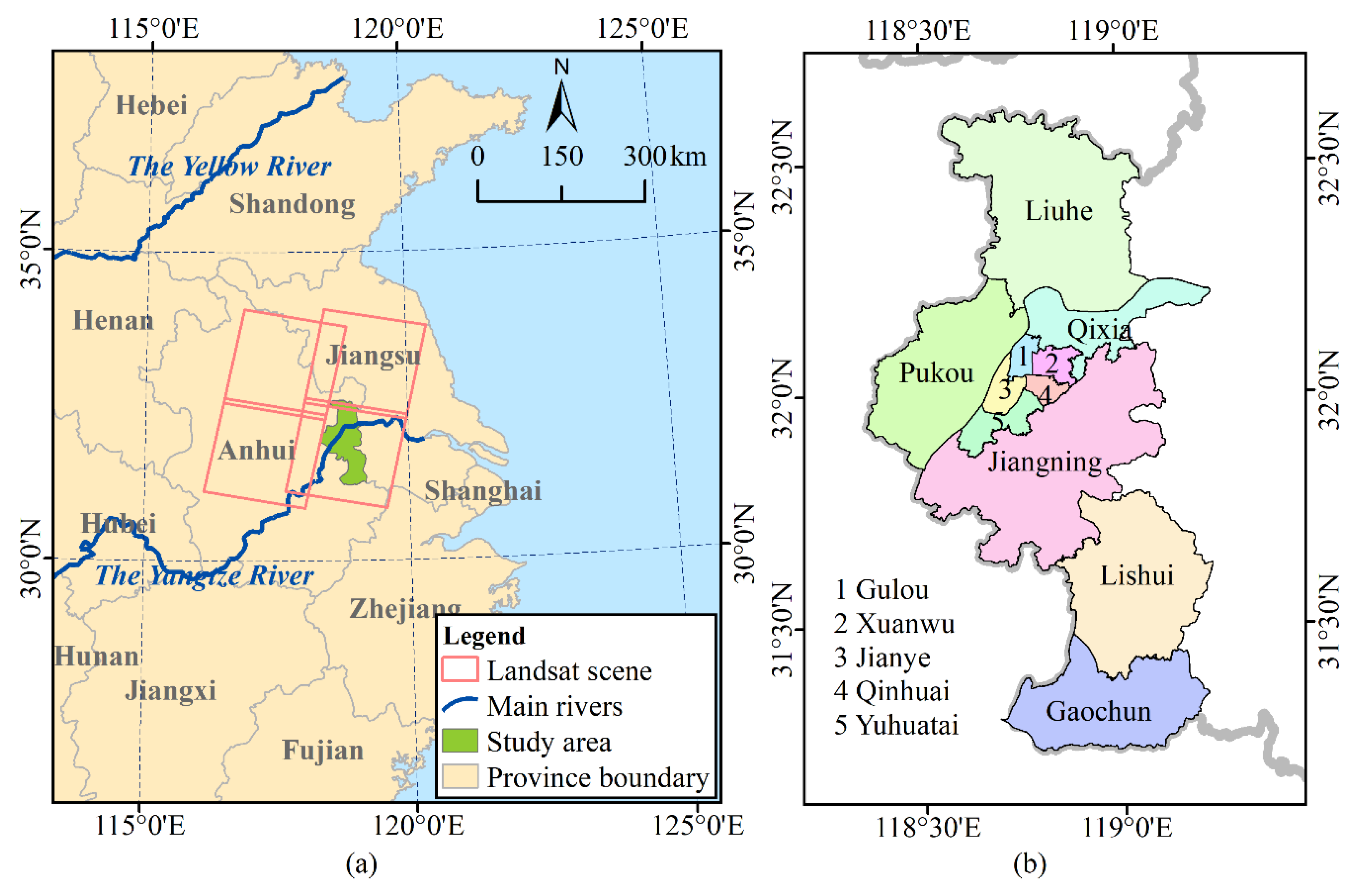
2.1. Study Area
2.2. Data
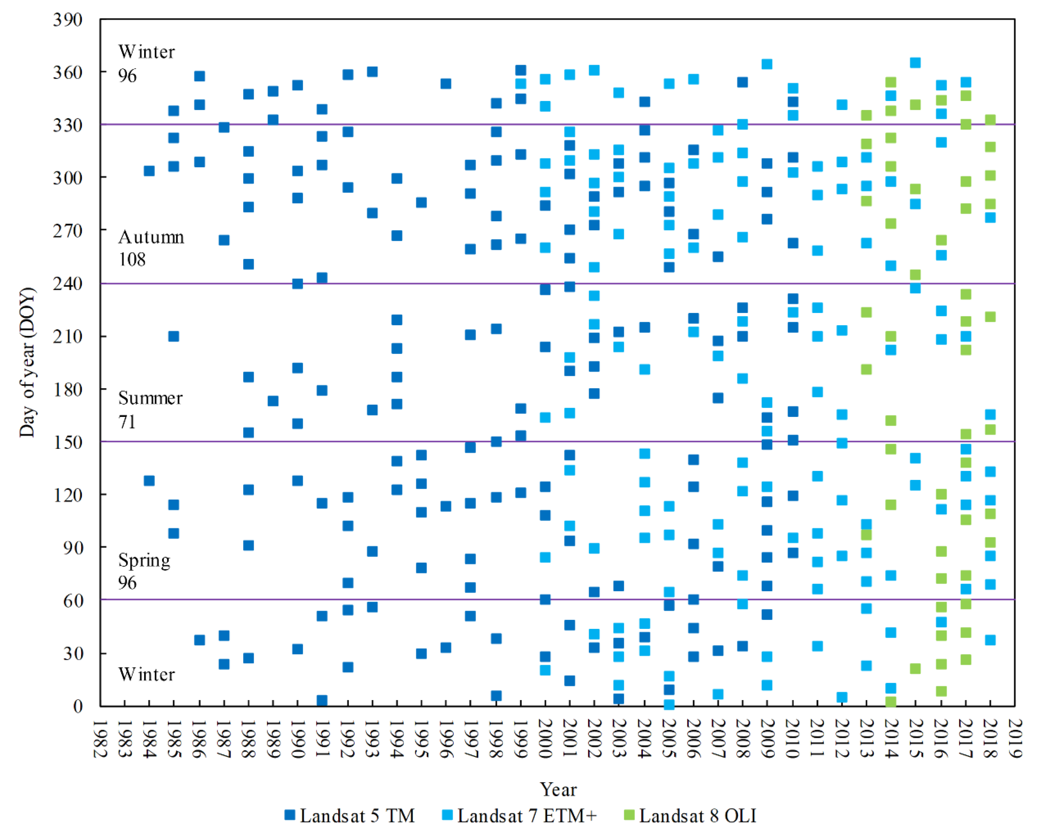
2.2.1. Landsat Data
2.2.2. Auxiliary Data
2.2.3. Other Open-Access Products
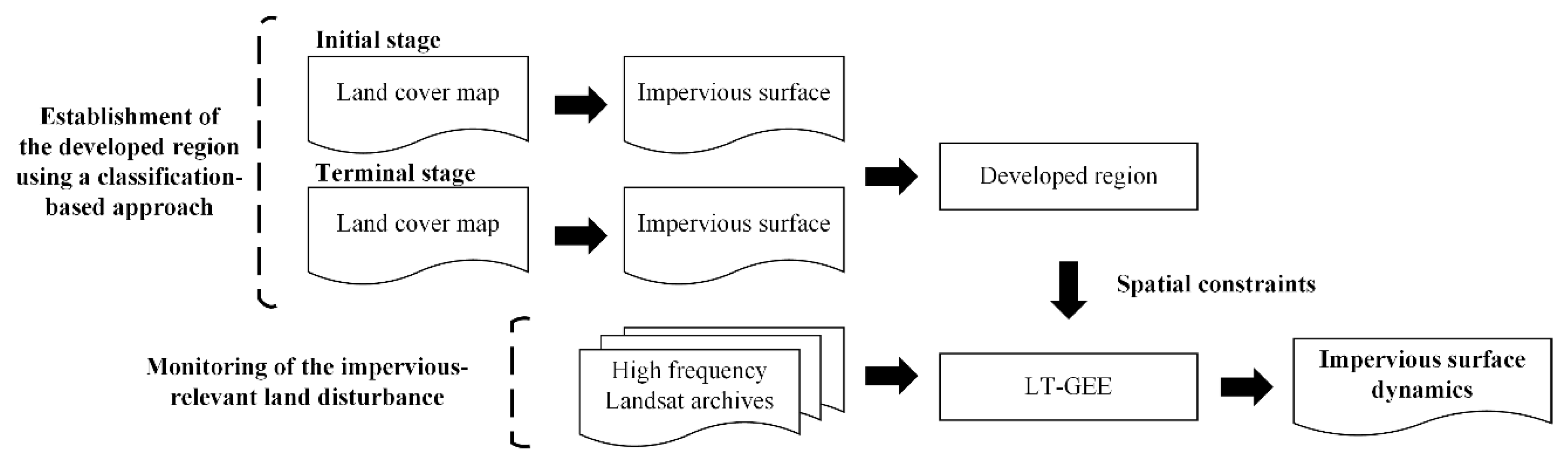
3. Methodology
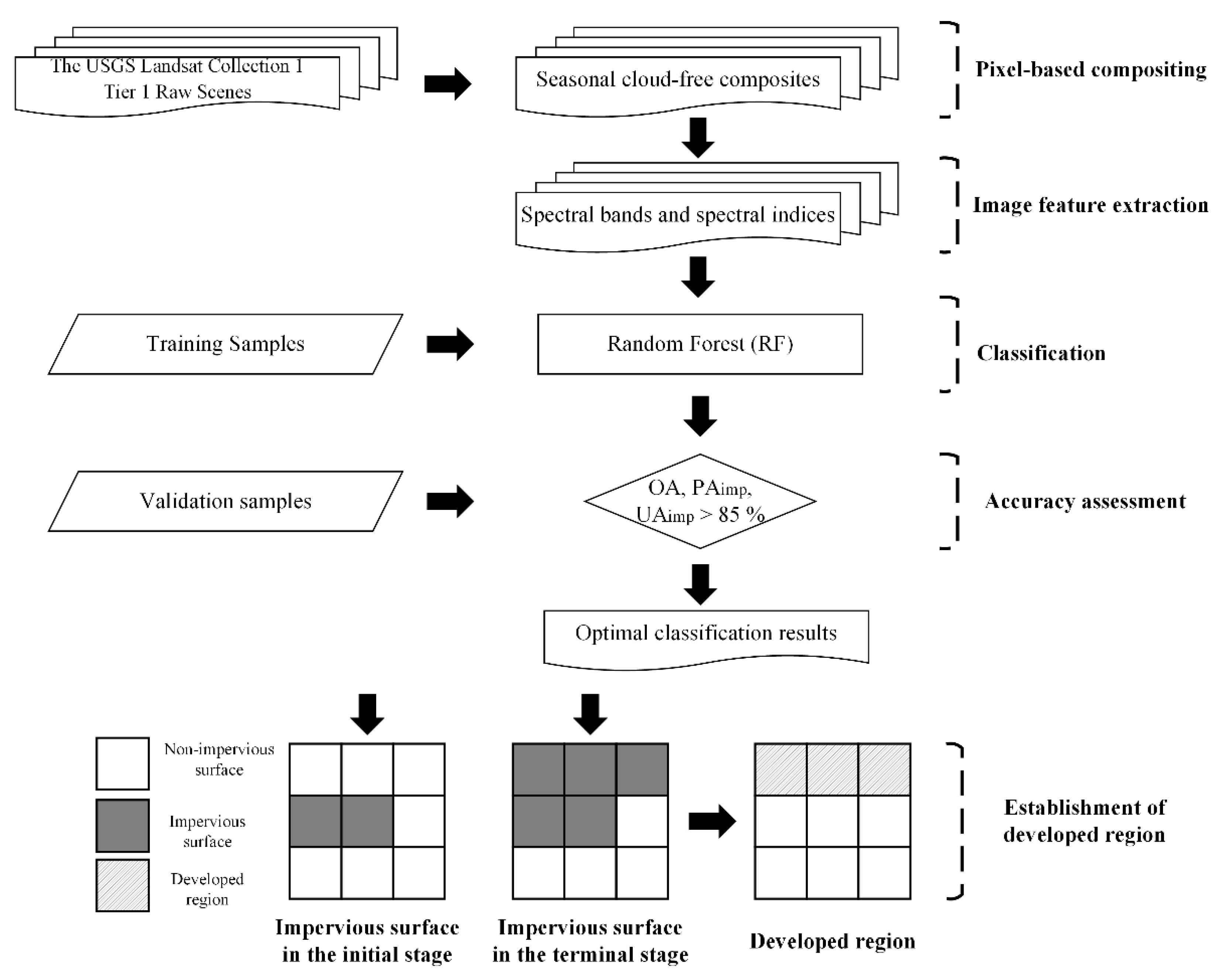
3.1. Establishment of the Developed Region Using a Classification-Based Approach
3.1.1. Pixel-Based Compositing
3.1.2. Feature Extraction and Classification Using RF
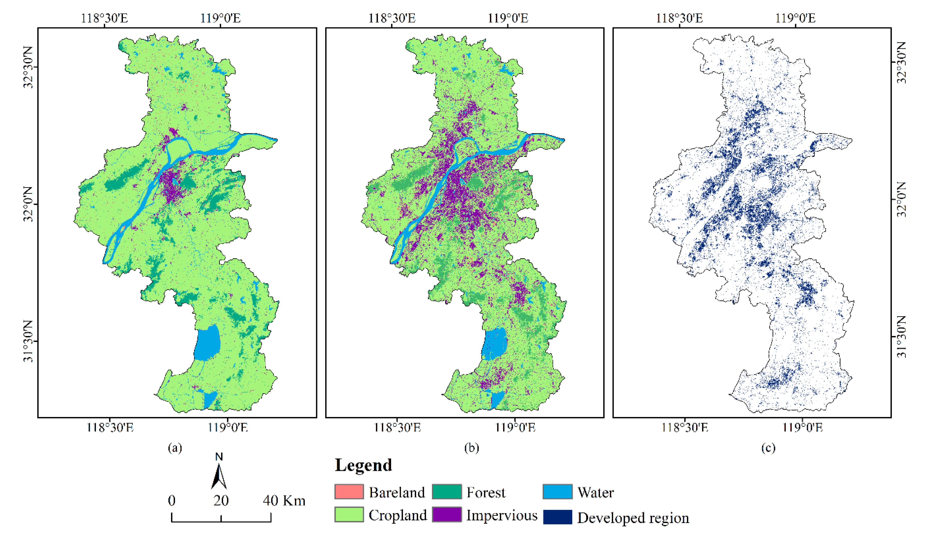
3.1.3. Establishment of the Developed Region
3.2. Monitoring of the Impervious–Relevant Land Disturbance
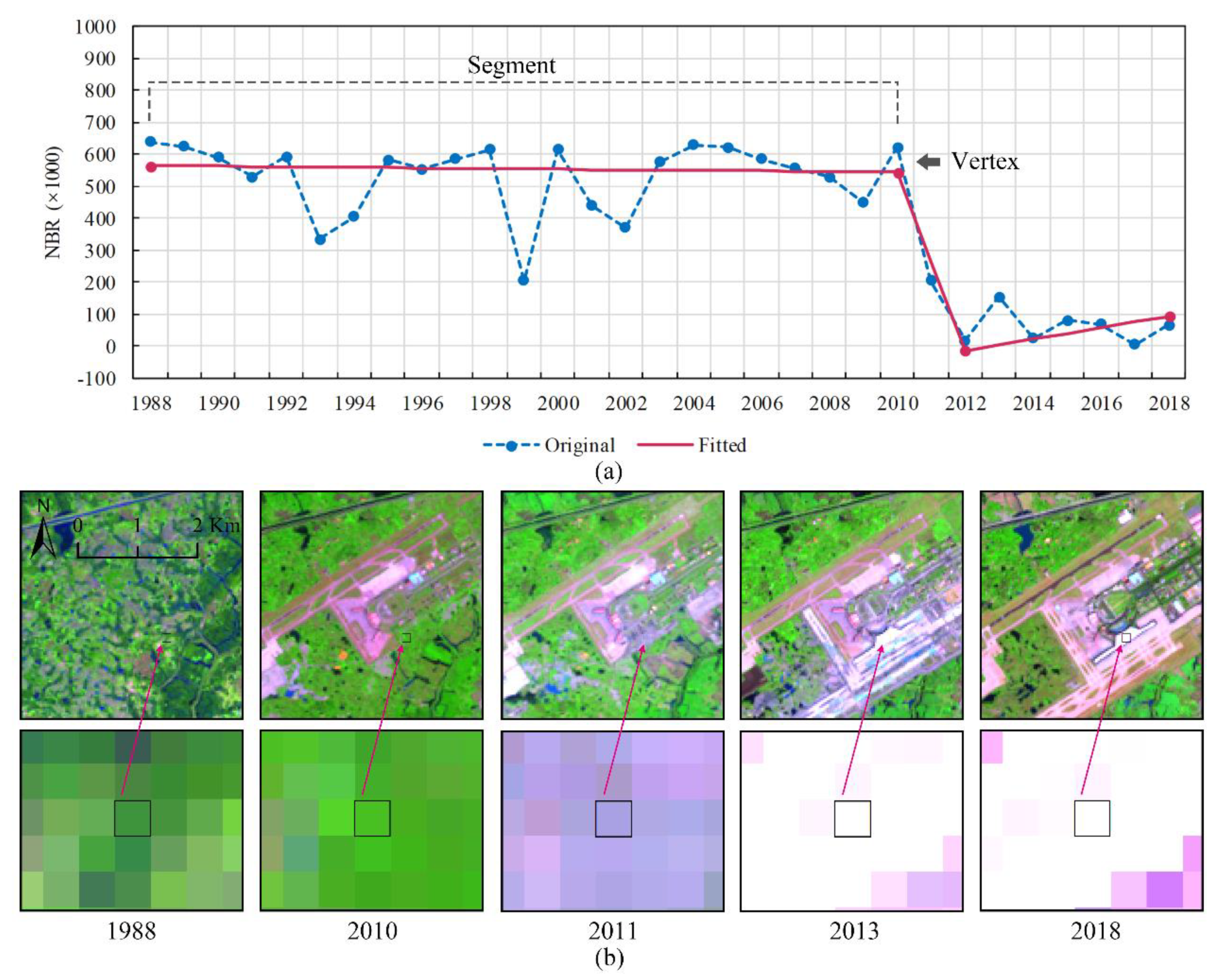
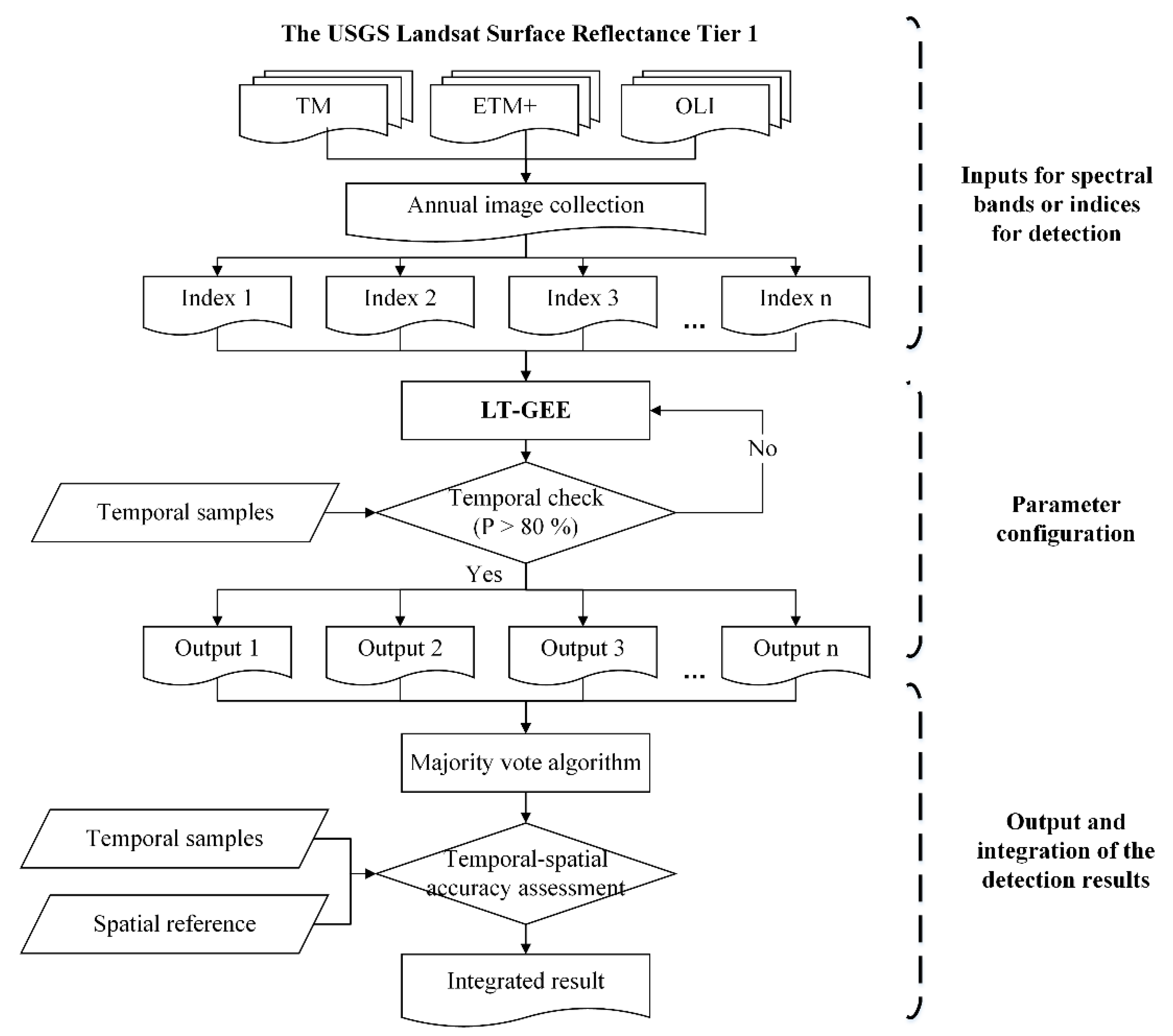
3.2.1. LT-GEE Algorithm
- The construction of an annual image collection:
- Parameter setting and trajectory segmentation:
3.2.2. Change Detection Framework for Impervious–relevant Land Disturbances
3.3. Accuracy Assessment
3.3.1. Accuracy Assessment for Classification
3.3.2. Accuracy Assessment for Change Detection
4. Results
4.1. Classification Results and the Developed Region
4.2. Change Detection Results
4.2.1. Optimal Parameter Configurations
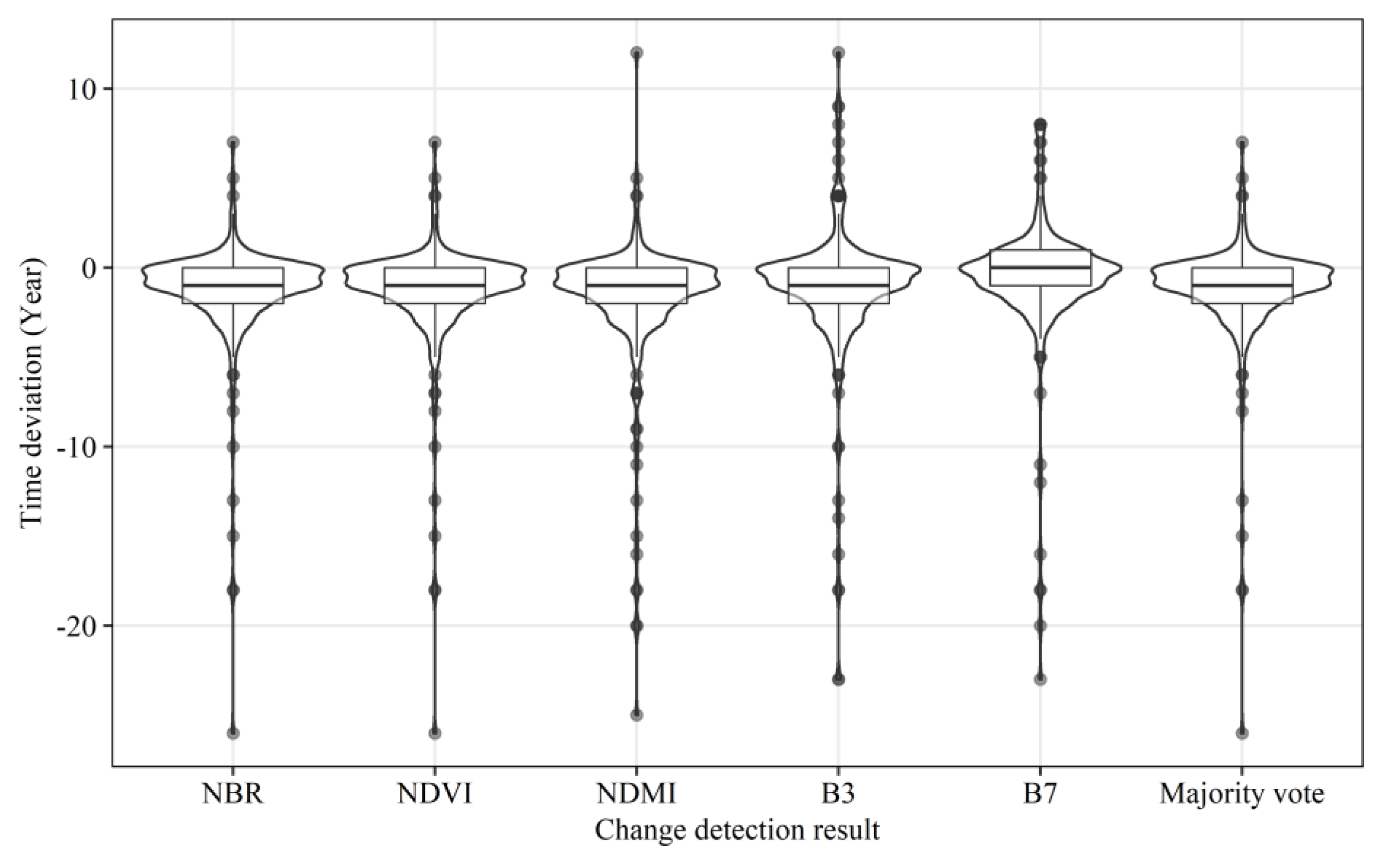
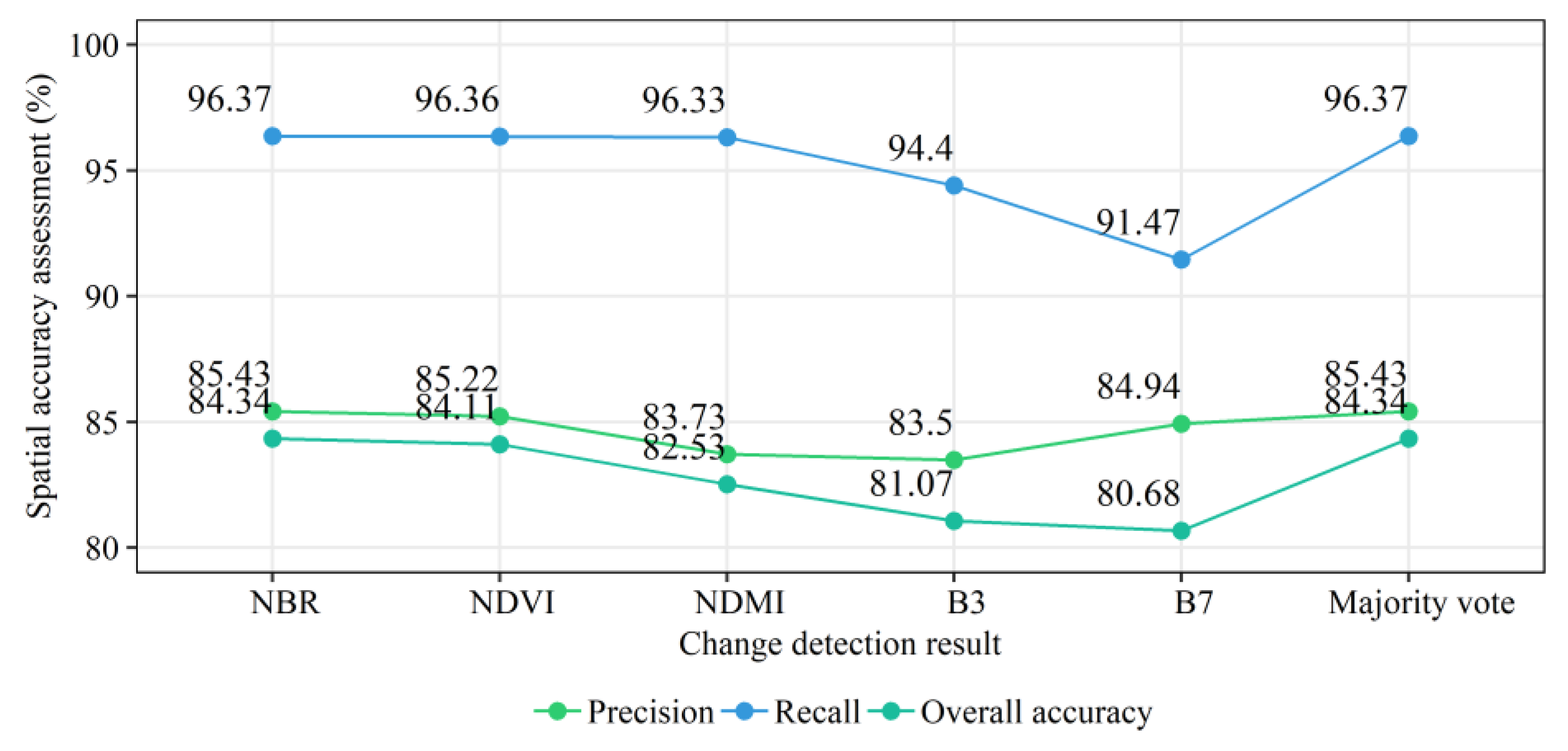
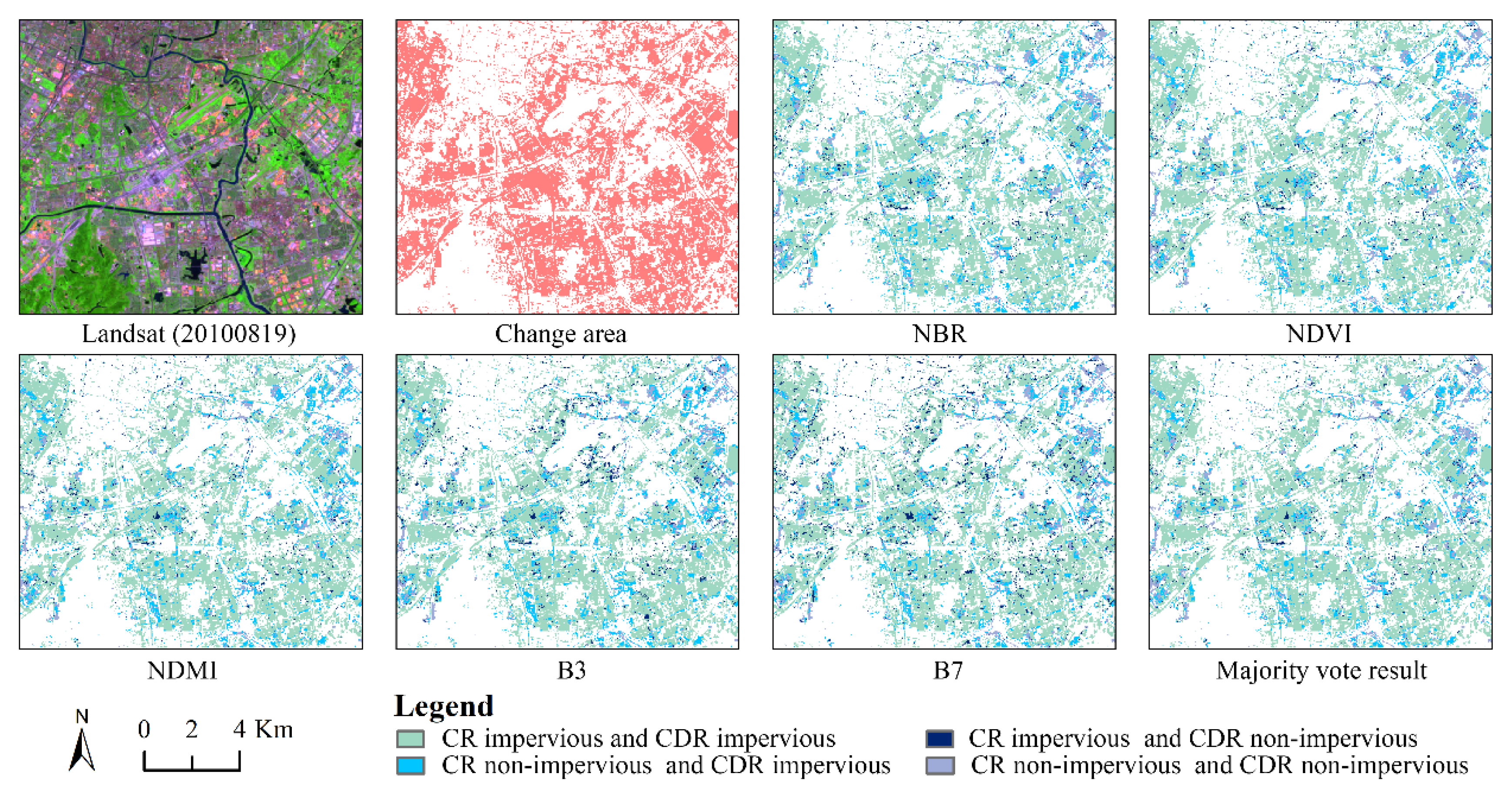
4.2.2. Change Detection Results and Quantitative Evaluations
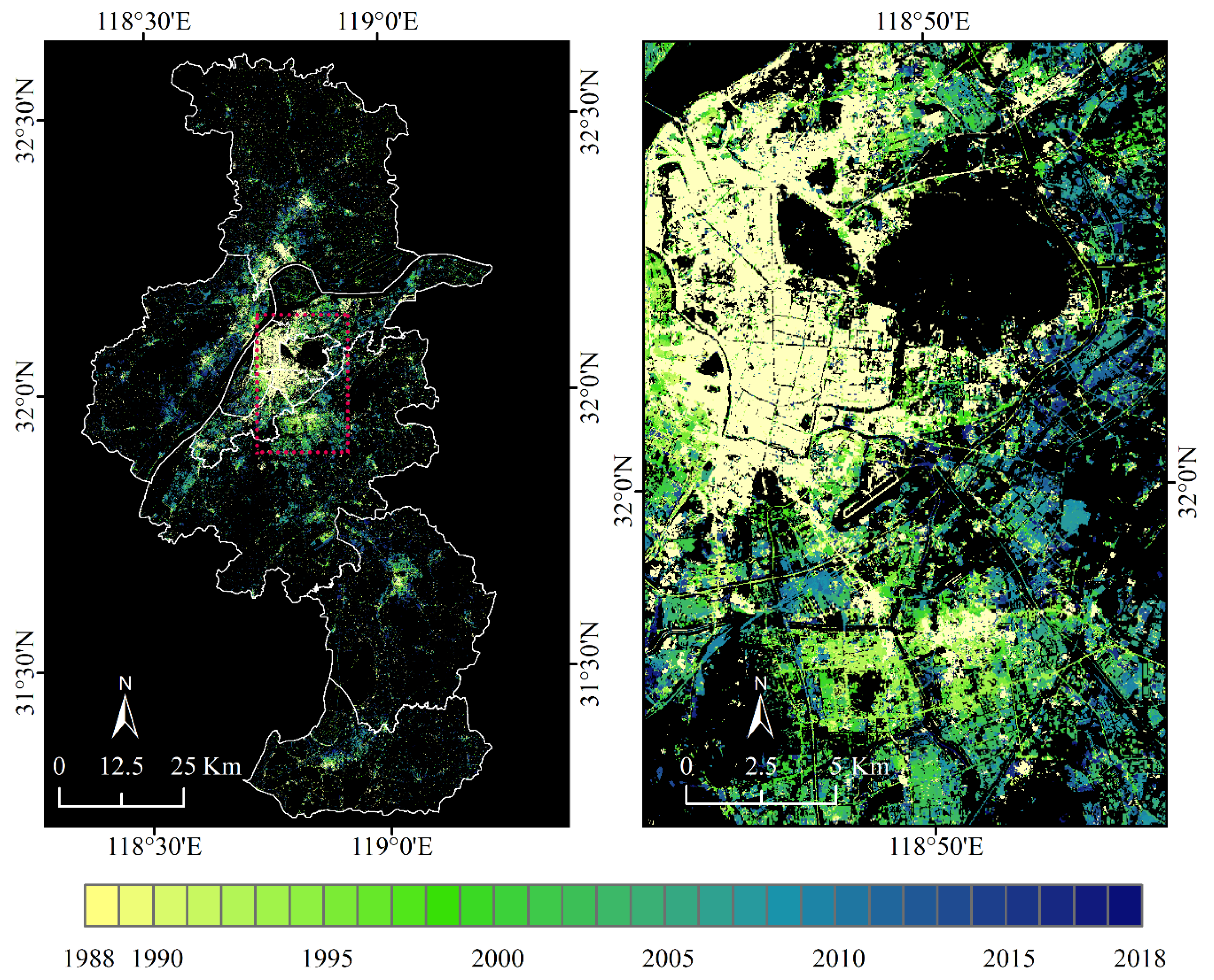
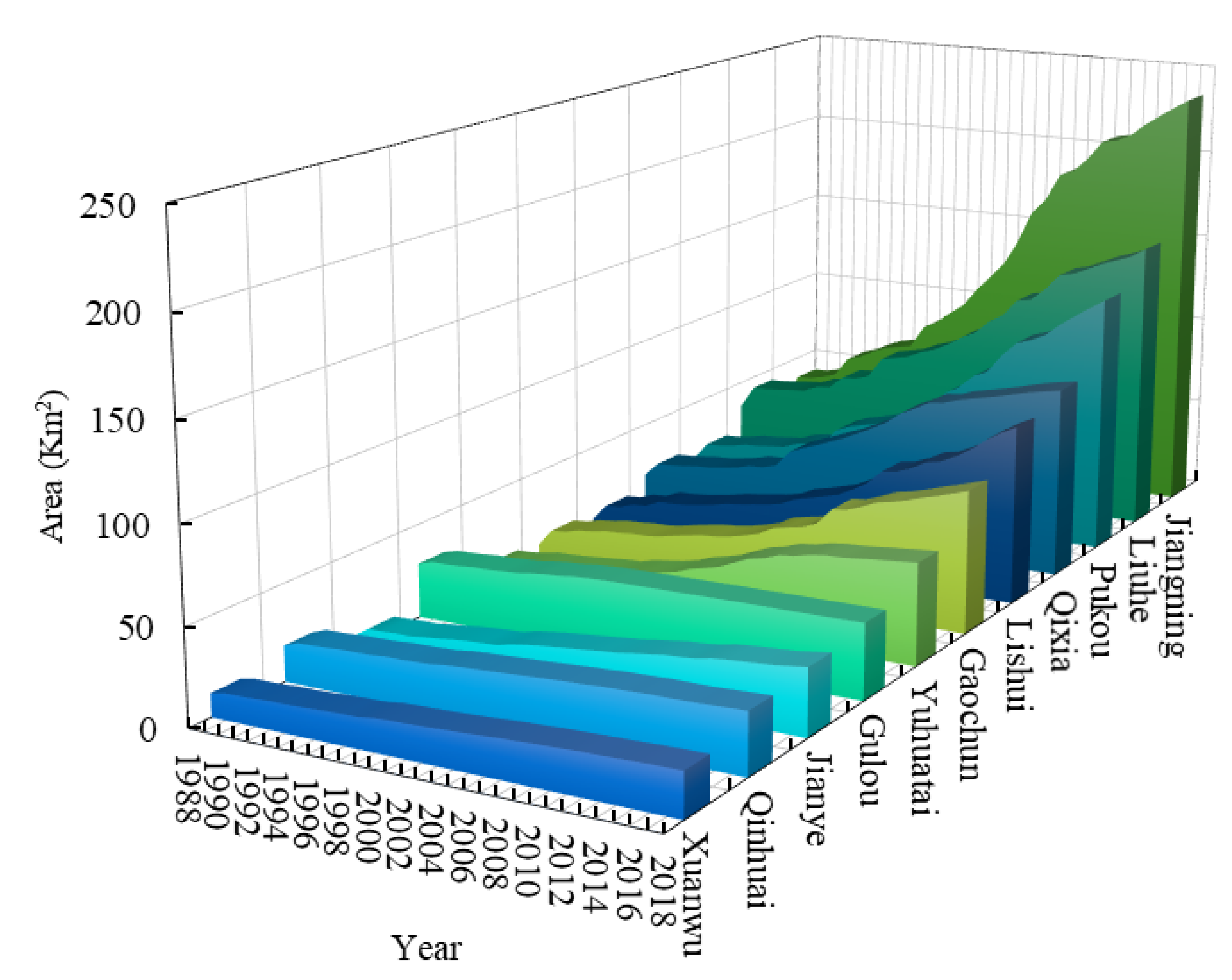
4.3. Expansion of Impervious Surface Dynamics in Nanjing
5. Discussions
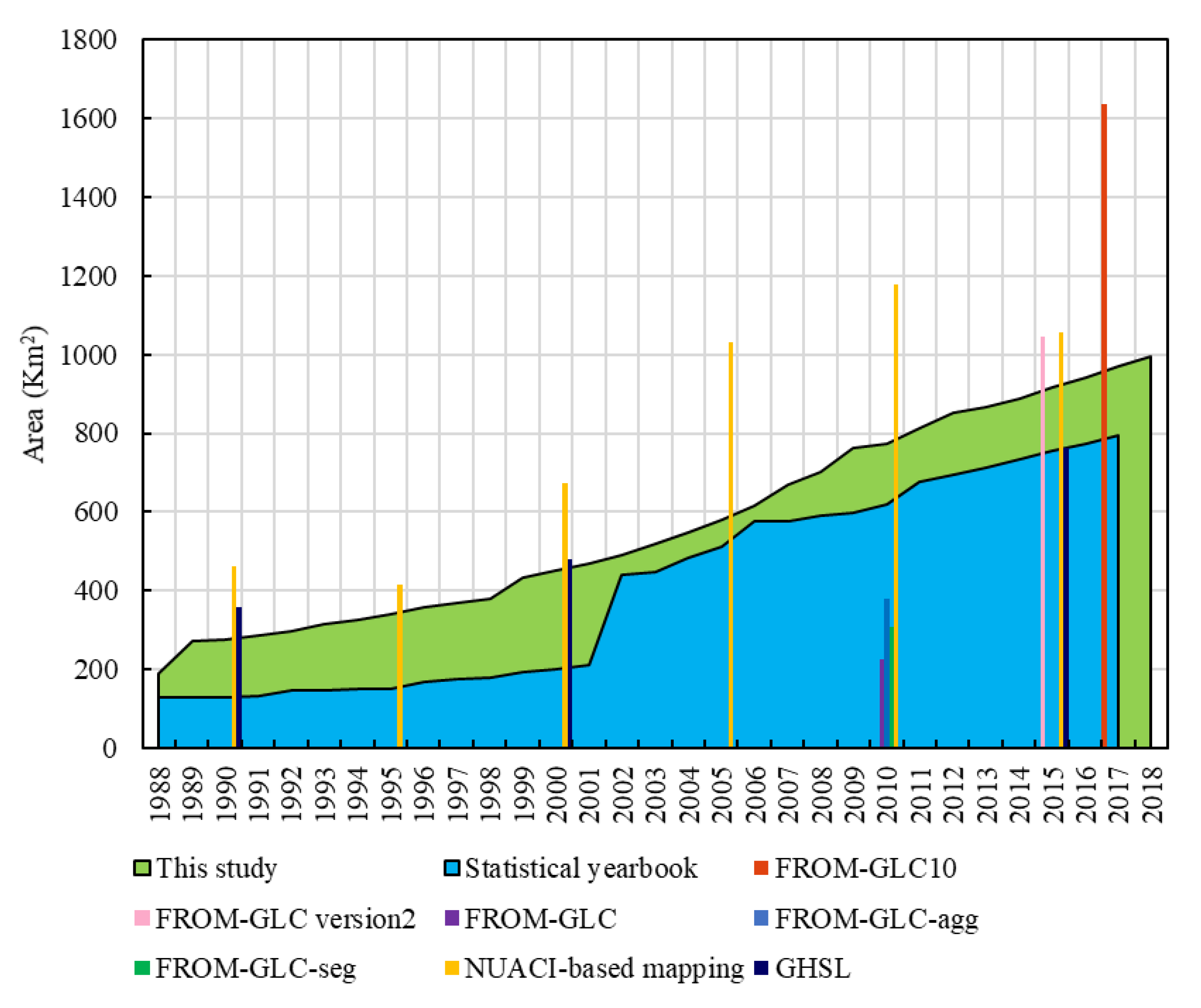
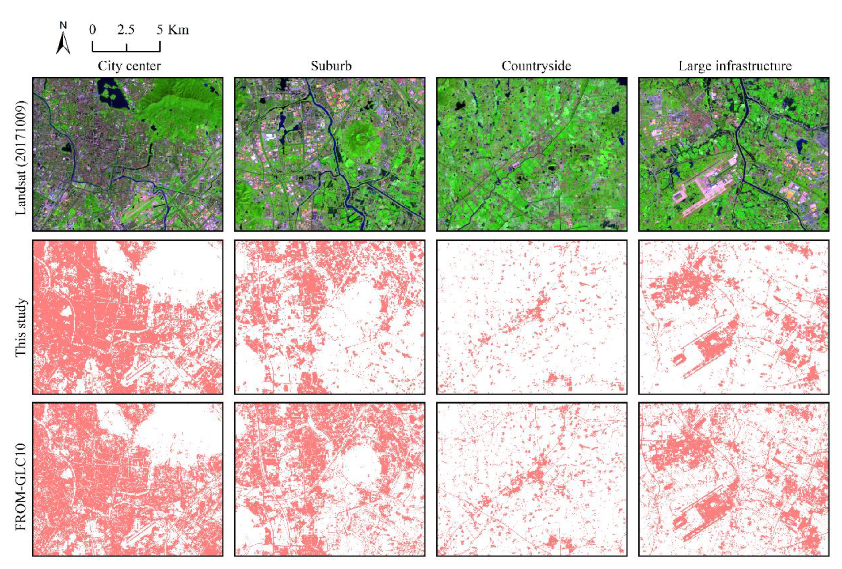
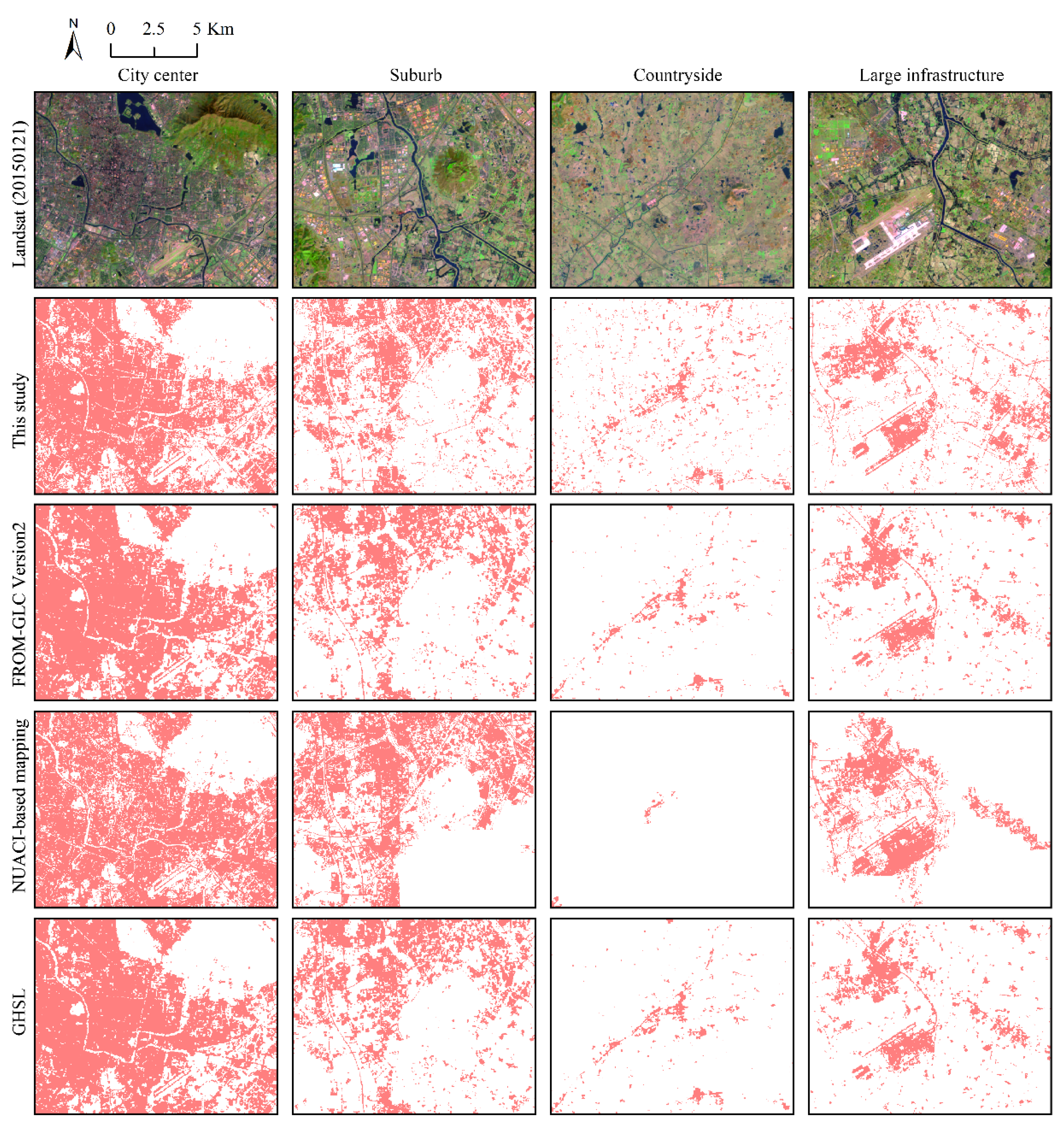
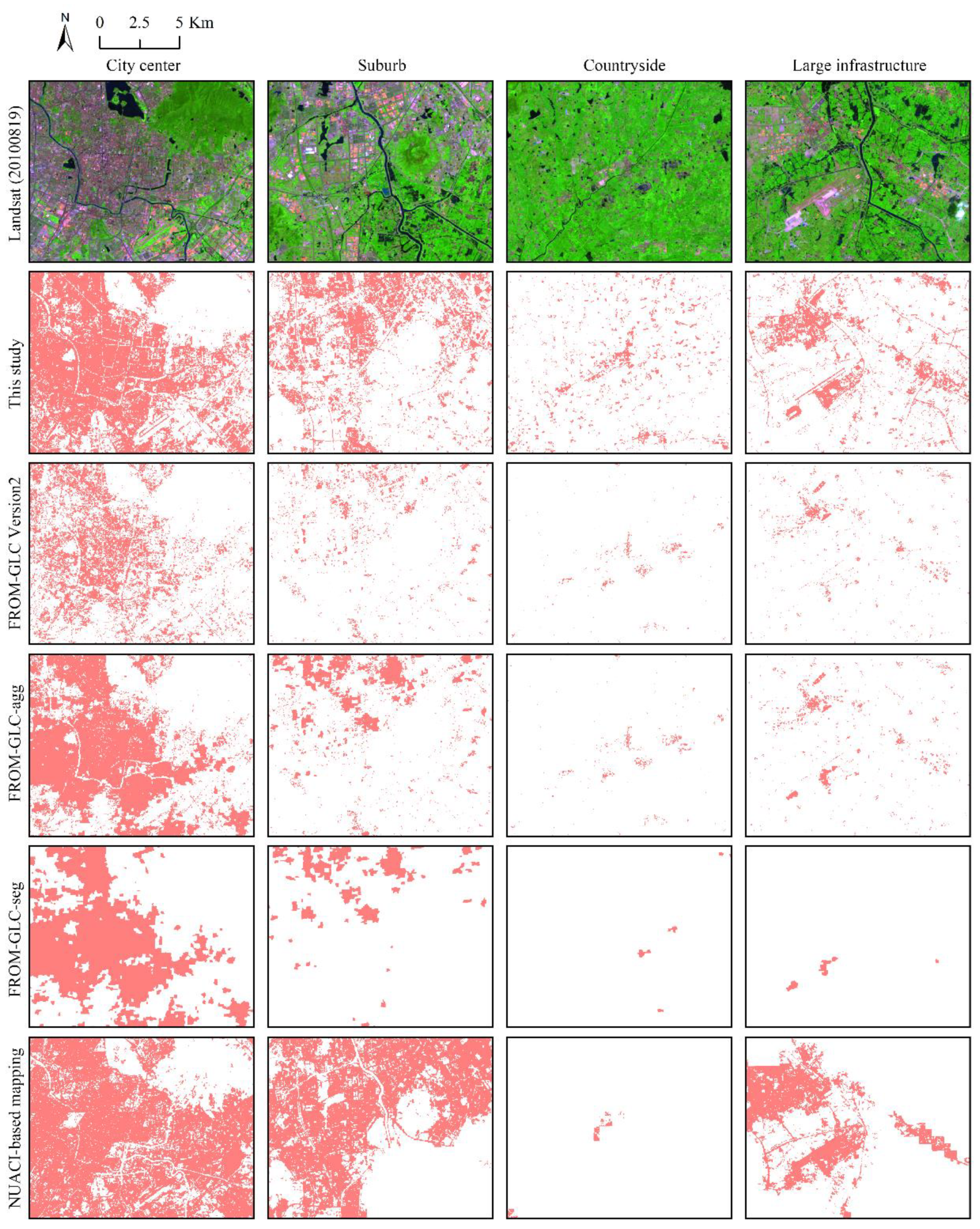
5.1. Comparisons with Other Open-Access Products
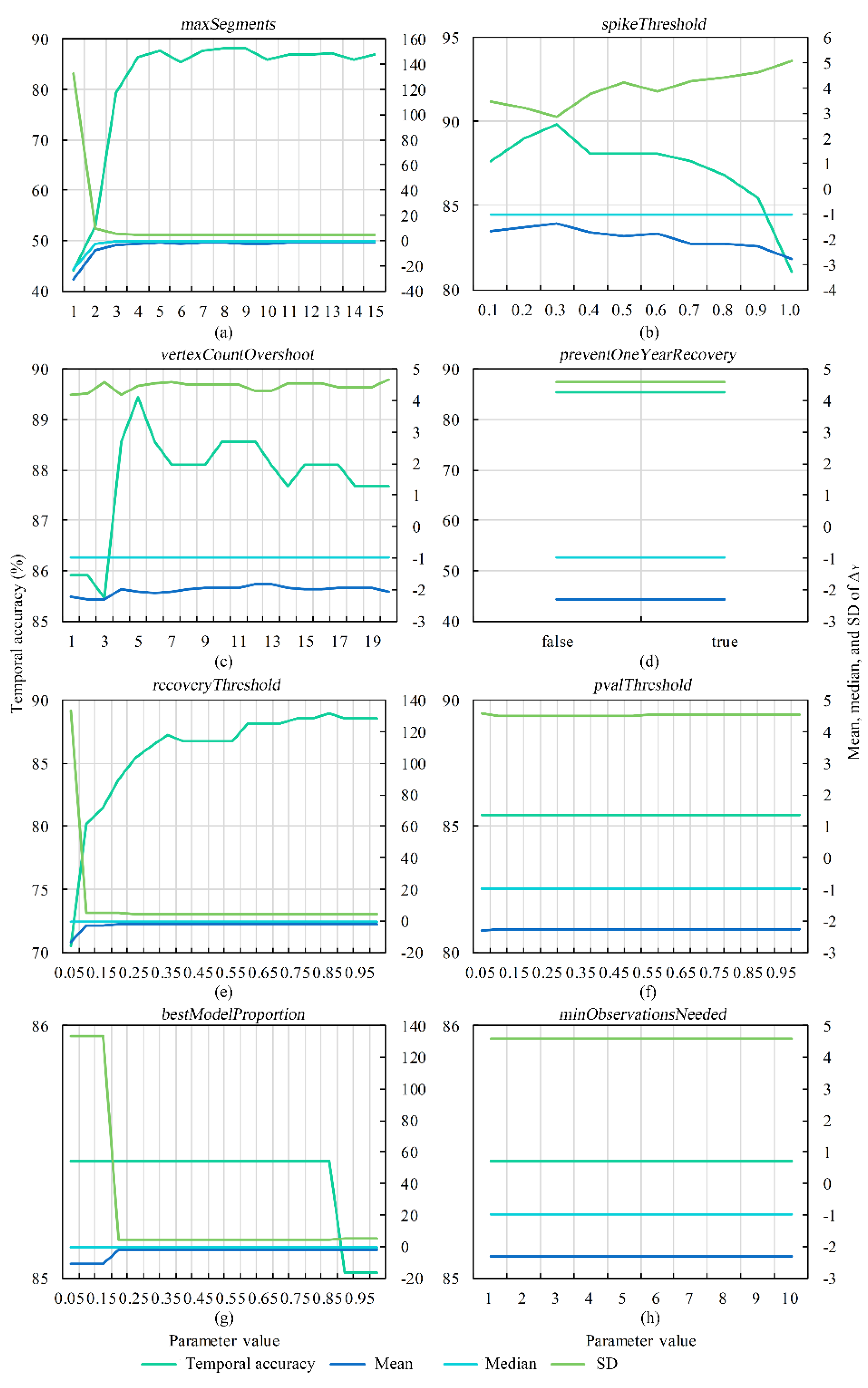
5.2. Parameter Sensitivity to the Output
5.3. The Proposed Scheme and Future Work
6. Conclusions
Author Contributions
Funding
Acknowledgments
Conflicts of Interest
Appendix A

| Data | Year | Data Structures | Method | Coverage | Reference |
|---|---|---|---|---|---|
| FROM-GLC10 | 2017 | Raster (10 m) | Pixel-based Classification | Global | [36] |
| FROM-GLC Version2 | 2015 | Raster (30 m) | Pixel-based Classification | Global | [49] |
| FROM-GLC | 2010 | Raster (30 m) | Pixel-based Classification | Global | [27] |
| FROM-GLC-agg | 2010 | Raster (30 m) | Multisource data aggregation | Global | [48] |
| FROM-GLC-seg | 2010 | Raster (30 m) | A segmentation-based approach | Global | [47] |
| NUACI-based mapping | 1990, 1995, 2000, 2005, 2010, 2015 | Raster (30 m) | NUACI-based classification | Global | [21] |
| GHSL | 1975, 1990, 2000, 2015 | Raster (30 m) | A classification based on symbolic machine learning | Global | [50] |
| China city statistical yearbook | 1985–2010 | Records | Statistical methods | China | [51] |
| Jiangsu statistical yearbook | 2011–2018 | Records | Statistical methods | Jiangsu | [52] |
| Nanjing statistical yearbook | 1978–2018 | Records | Statistical methods | Nanjing | [42] |
| Parameter | Type | Definition | Default |
|---|---|---|---|
| startYear | Integer | The initial year of detection duration | 1984 |
| endYear | Integer | The terminal year of detection duration | 2017 |
| startDay | Integer | The time of initial year | 0620 |
| endDay | Integer | The time of terminal year | 0910 |
| index | String | The first band in the image collection and generate annual fitted-to-vertex (FTV) data for each subsequent band | NBR |
| maxSegments | Integer | Maximum number of segments to be fitted on the time series | 6 |
| spikeThreshold | Float | Threshold for dampening the spikes (1.0 means no dampening) | 0.9 |
| vertexCountOvershoot | Integer | The initial model can overshoot the maxSegments + 1 vertices by this amount. Later, it will be pruned down to maxSegments + 1 | 3 |
| preventOneYearRecovery | Boolean | Prevent segments that represent one year recoveries | true |
| recoveryThreshold | Float | If a segment has a recovery rate faster than 1/recoveryThreshold (in years), then the segment is disallowed | 0.25 |
| pvalThreshold | Float | If the p-value of the fitted model exceeds this threshold, then the current model is discarded and another one is fitted using the Levenberg-Marquardt optimizer | 0.05 |
| bestModelProportion | Float | Takes the model with most vertices that has a p-value that is at most this proportion away from the model with lowest p-value | 0.75 |
| minObservationsNeeded | Integer | Minimum observations needed to perform output fitting | 6 |
| timeSeries | ImageCollection | Collection from which to extract trends (it is assumed that each image in the collection represents one year). The first band is used to find breakpoints, and all subsequent bands are fitted using those breakpoints | |
| delta | String | Vegetation change type, ensure that the band or index to be segmented is oriented with vegetation “loss” and “gain” | lose |
| sort | String | Vegetation change sort, which contains “Least”, “Newest”, “Greatest”, “Oldest”, “Fastest”, and “Slowest” | greatest |
| year | Boolean, Integer | Filter detection result by year of detection | checked: true, start: 1986, end: 2017 |
| mag | Boolean, Integer, String | Filter detection result by magnitude | checked: true, value: 200, operator: ‘>’ |
| dur | Boolean, Integer, String | Filter detection result by change event duration | checked: true, value: 4, operator: ‘<’ |
| preval | Boolean, Integer, String | Filter detection result by pre-change spectral value | checked: true, value: 300, operator: ‘>’ |
| mmu | Boolean, Integer | Filter detection result by minimum mapping patch unit | checked: true, value: 11 |
References
- Montgomery, M.R. The Urban Transformation of the Developing World. Science 2008, 319, 761–764. [Google Scholar] [CrossRef] [PubMed] [Green Version]
- Schneider, A.; Friedl, M.A.; Potere, D. Mapping global urban areas using MODIS 500-m data: New methods and datasets based on ‘urban ecoregions’. Remote Sens. Environ. 2010, 114, 1733–1746. [Google Scholar] [CrossRef]
- Seto, K.C.; Güneralp, B.; Hutyra, L.R. Global forecasts of urban expansion to 2030 and direct impacts on biodiversity and carbon pools. Proc. Natl. Acad. Sci. USA 2012, 109, 16083–16088. [Google Scholar] [CrossRef] [PubMed] [Green Version]
- Schneider, A.; Mertes, C.M.; Tatem, A.J.; Tan, B.; Sulla-Menashe, D.; Graves, S.J.; Patel, N.N.; Horton, J.A.; Gaughan, A.E.; Rollo, J.T.; et al. A new urban landscape in East–Southeast Asia, 2000–2010. Environ. Res. Lett. 2015, 10, 034002. [Google Scholar] [CrossRef]
- Zhou, Y.; Li, X.; Asrar, G.R.; Smith, S.J.; Imhoff, M. A global record of annual urban dynamics (1992–2013) from nighttime lights. Remote Sens. Environ. 2018, 219, 206–220. [Google Scholar] [CrossRef]
- Gong, P.; Li, X.; Zhang, W. 40-year (1978-2017) human settlement changes in China reflected by impervious surfaces from satellite remote sensing. Sci. Bull. 2019, 64, 756–763. [Google Scholar] [CrossRef]
- Arnold, C.L.; Gibbons, C.J. Impervious Surface Coverage: The Emergence of a Key Environmental Indicator. J. Am. Plan. Assoc. 1996, 62, 243–258. [Google Scholar] [CrossRef]
- Weng, Q. Remote sensing of impervious surfaces in the urban areas: Requirements, methods, and trends. Remote Sens. Environ. 2012, 117, 34–49. [Google Scholar] [CrossRef]
- Liu, C.; Zhang, Q.; Luo, H.; Qi, S.; Tao, S.; Xu, H.; Yao, Y. An efficient approach to capture continuous impervious surface dynamics using spatial-temporal rules and dense Landsat time series stacks. Remote Sens. Environ. 2019, 229, 114–132. [Google Scholar] [CrossRef]
- Deng, C.; Zhu, Z. Continuous subpixel monitoring of urban impervious surface using Landsat time series. Remote Sens. Environ. 2018. [Google Scholar] [CrossRef]
- Zhang, L.; Weng, Q. Annual dynamics of impervious surface in the Pearl River Delta, China, from 1988 to 2013, using time series Landsat imagery. ISPRS J. Photogramm. Remote Sens. 2016, 113, 86–96. [Google Scholar] [CrossRef]
- Weng, Q.; Rajasekar, U.; Hu, X. Modeling Urban Heat Islands and Their Relationship with Impervious Surface and Vegetation Abundance by Using ASTER Images. IEEE Trans. Geosci. Remote Sens. 2011, 49, 4080–4089. [Google Scholar] [CrossRef]
- Carlson, T.N.; Arthur, S.T. The impact of land use—Land cover changes due to urbanization on surface microclimate and hydrology: A satellite perspective. Glob. Planet. Chang. 2000, 25, 49–65. [Google Scholar] [CrossRef]
- Qin, Y.; Xiao, X.; Dong, J.; Chen, B.; Liu, F.; Zhang, G.; Zhang, Y.; Wang, J.; Wu, X. Quantifying annual changes in built-up area in complex urban-rural landscapes from analyses of PALSAR and Landsat images. ISPRS J. Photogramm. Remote Sens. 2017, 124, 89–105. [Google Scholar] [CrossRef] [Green Version]
- Zhu, Z.; Zhou, Y.; Seto, K.C.; Stokes, E.C.; Deng, C.; Pickett, S.T.A.; Taubenböck, H. Understanding an urbanizing planet: Strategic directions for remote sensing. Remote Sens. Environ. 2019, 228, 164–182. [Google Scholar] [CrossRef]
- Fu, Y.; Li, J.; Weng, Q.; Zheng, Q.; Li, L.; Dai, S.; Guo, B. Characterizing the spatial pattern of annual urban growth by using time series Landsat imagery. Sci. Total Environ. 2019, 666, 274–284. [Google Scholar] [CrossRef]
- Schneider, A.; Mertes, C.M. Expansion and growth in Chinese cities, 1978–2010. Environ. Res. Lett. 2014, 9, 024008. [Google Scholar] [CrossRef]
- Zhu, Z.; Wulder, M.A.; Roy, D.P.; Woodcock, C.E.; Hansen, M.C.; Radeloff, V.C.; Healey, S.P.; Schaaf, C.; Hostert, P.; Strobl, P.; et al. Benefits of the free and open Landsat data policy. Remote Sens. Environ. 2019, 224, 382–385. [Google Scholar] [CrossRef]
- Wulder, M.A.; Loveland, T.R.; Roy, D.P.; Crawford, C.J.; Masek, J.G.; Woodcock, C.E.; Allen, R.G.; Anderson, M.C.; Belward, A.S.; Cohen, W.B.; et al. Current status of Landsat program, science, and applications. Remote Sens. Environ. 2019, 225, 127–147. [Google Scholar] [CrossRef]
- Woodcock, C.E.; Allen, R.; Anderson, M.; Belward, A.; Bindschadler, R.; Cohen, W.; Gao, F.; Goward, S.N.; Helder, D.; Helmer, E.; et al. Free Access to Landsat Imagery. Science 2008, 320, 1011. [Google Scholar] [CrossRef]
- Liu, X.; Hu, G.; Chen, Y.; Li, X.; Xu, X.; Li, S.; Pei, F.; Wang, S. High-resolution multi-temporal mapping of global urban land using Landsat images based on the Google Earth Engine Platform. Remote Sens. Environ. 2018, 209, 227–239. [Google Scholar] [CrossRef]
- Zhu, Z.; Woodcock, C.E. Object-based cloud and cloud shadow detection in Landsat imagery. Remote Sens. Environ. 2012, 118, 83–94. [Google Scholar] [CrossRef]
- Zhu, Z. Change detection using landsat time series: A review of frequencies, preprocessing, algorithms, and applications. ISPRS J. Photogramm. Remote Sens. 2017, 130, 370–384. [Google Scholar] [CrossRef]
- Wulder, M.A.; Coops, N.C.; Roy, D.P.; White, J.C.; Hermosilla, T. Land cover 2.0. Int. J. Remote Sens. 2018, 39, 4254–4284. [Google Scholar] [CrossRef] [Green Version]
- Belgiu, M.; Drăguţ, L. Random forest in remote sensing: A review of applications and future directions. ISPRS J. Photogramm. Remote Sens. 2016, 114, 24–31. [Google Scholar] [CrossRef]
- Breiman, L. Random Forests. Mach. Learn. 2001, 45, 5–32. [Google Scholar] [CrossRef] [Green Version]
- Gong, P.; Wang, J.; Yu, L.; Zhao, Y.; Zhao, Y.; Liang, L.; Niu, Z.; Huang, X.; Fu, H.; Liu, S.; et al. Finer resolution observation and monitoring of global land cover: First mapping results with Landsat TM and ETM+ data. Int. J. Remote Sens. 2013, 34, 2607–2654. [Google Scholar] [CrossRef]
- Li, X.; Gong, P.; Liang, L. A 30-year (1984–2013) record of annual urban dynamics of Beijing City derived from Landsat data. Remote Sens. Environ. 2015, 166, 78–90. [Google Scholar] [CrossRef]
- Xu, H.; Qi, S.; Gong, P.; Liu, C.; Wang, J. Long-term monitoring of citrus orchard dynamics using time-series Landsat data: A case study in southern China. Int. J. Remote Sens. 2018, 39, 8271–8292. [Google Scholar] [CrossRef]
- Huang, C.; Goward, S.N.; Masek, J.G.; Thomas, N.; Zhu, Z.; Vogelmann, J.E. An automated approach for reconstructing recent forest disturbance history using dense Landsat time series stacks. Remote Sens. Environ. 2010, 114, 183–198. [Google Scholar] [CrossRef]
- Kennedy, R.E.; Yang, Z.; Cohen, W.B. Detecting trends in forest disturbance and recovery using yearly Landsat time series: 1. LandTrendr—Temporal segmentation algorithms. Remote Sens. Environ. 2010, 114, 2897–2910. [Google Scholar] [CrossRef]
- Brooks, E.B.; Wynne, R.H.; Thomas, V.A.; Blinn, C.E.; Coulston, J.W. On-the-Fly Massively Multitemporal Change Detection Using Statistical Quality Control Charts and Landsat Data. IEEE Trans. Geosci. Remote Sens. 2014, 52, 3316–3332. [Google Scholar] [CrossRef]
- Zhu, Z.; Woodcock, C.E. Continuous change detection and classification of land cover using all available Landsat data. Remote Sens. Environ. 2014, 144, 152–171. [Google Scholar] [CrossRef] [Green Version]
- Zhu, Z.; Zhang, J.; Yang, Z.; Aljaddani, A.H.; Cohen, W.B.; Qiu, S.; Zhou, C. Continuous monitoring of land disturbance based on Landsat time series. Remote Sens. Environ. 2019. [Google Scholar] [CrossRef]
- Gorelick, N.; Hancher, M.; Dixon, M.; Ilyushchenko, S.; Thau, D.; Moore, R. Google Earth Engine: Planetary-scale geospatial analysis for everyone. Remote Sens. Environ. 2017, 202, 18–27. [Google Scholar] [CrossRef]
- Gong, P.; Liu, H.; Zhang, M.; Li, C.; Wang, J.; Huang, H.; Clinton, N.; Ji, L.; Li, W.; Bai, Y.; et al. Stable classification with limited sample: Transferring a 30-m resolution sample set collected in 2015 to mapping 10-m resolution global land cover in 2017. Sci. Bull. 2019, 64, 370–373. [Google Scholar] [CrossRef]
- Kennedy, R.E.; Yang, Z.; Gorelick, N.; Braaten, J.; Cavalcante, L.; Cohen, W.B.; Healey, S. Implementation of the LandTrendr Algorithm on Google Earth Engine. Remote Sens. 2018, 10, 691. [Google Scholar] [CrossRef]
- Huang, H.; Chen, Y.; Clinton, N.; Wang, J.; Wang, X.; Liu, C.; Gong, P.; Yang, J.; Bai, Y.; Zheng, Y.; et al. Mapping major land cover dynamics in Beijing using all Landsat images in Google Earth Engine. Remote Sens. Environ. 2017, 202, 166–176. [Google Scholar] [CrossRef]
- Hao, B.; Ma, M.; Li, S.; Li, Q.; Hao, D.; Huang, J.; Ge, Z.; Yang, H.; Han, X. Land Use Change and Climate Variation in the Three Gorges Reservoir Catchment from 2000 to 2015 Based on the Google Earth Engine. Sensors 2019, 19, 2118. [Google Scholar] [CrossRef]
- Cohen, B.W.; Healey, P.S.; Yang, Z.; Stehman, V.S.; Brewer, K.C.; Brooks, B.E.; Gorelick, N.; Huang, C.; Hughes, J.M.; Kennedy, E.R.; et al. How Similar Are Forest Disturbance Maps Derived from Different Landsat Time Series Algorithms? Forests 2017, 8, 98. [Google Scholar] [CrossRef]
- Kennedy, R.E.; Yang, Z.; Cohen, W.B.; Pfaff, E.; Braaten, J.; Nelson, P. Spatial and temporal patterns of forest disturbance and regrowth within the area of the Northwest Forest Plan. Remote Sens. Environ. 2012, 122, 117–133. [Google Scholar] [CrossRef]
- Nanjing Statistical Bureau. Nanjing Statistical Yearbook; Nanjing Statistical Bureau: Nanjing, China, 2018.
- Claverie, M.; Ju, J.; Masek, J.G.; Dungan, J.L.; Vermote, E.F.; Roger, J.-C.; Skakun, S.V.; Justice, C. The Harmonized Landsat and Sentinel-2 surface reflectance data set. Remote Sens. Environ. 2018, 219, 145–161. [Google Scholar] [CrossRef]
- Masek, J.G.; Vermote, E.F.; Saleous, N.E.; Wolfe, R.; Hall, F.G.; Huemmrich, K.F.; Feng, G.; Kutler, J.; Teng-Kui, L. A Landsat surface reflectance dataset for North America, 1990–2000. IEEE Geosci. Remote Sens. Lett. 2006, 3, 68–72. [Google Scholar] [CrossRef]
- Vermote, E.; Justice, C.; Claverie, M.; Franch, B. Preliminary analysis of the performance of the Landsat 8/OLI land surface reflectance product. Remote Sens. Environ. 2016, 185, 46–56. [Google Scholar] [CrossRef]
- Grinand, C.; Rakotomalala, F.; Gond, V.; Vaudry, R.; Bernoux, M.; Vieilledent, G. Estimating deforestation in tropical humid and dry forests in Madagascar from 2000 to 2010 using multi-date Landsat satellite images and the random forests classifier. Remote Sens. Environ. 2013, 139, 68–80. [Google Scholar] [CrossRef]
- Yu, L.; Wang, J.; Gong, P. Improving 30 m global land-cover map FROM-GLC with time series MODIS and auxiliary data sets: A segmentation-based approach. Int. J. Remote Sens. 2013, 34, 5851–5867. [Google Scholar] [CrossRef]
- Yu, L.; Wang, J.; Li, X.; Li, C.; Zhao, Y.; Gong, P. A multi-resolution global land cover dataset through multisource data aggregation. Sci. China Earth Sci. 2014, 57, 2317–2329. [Google Scholar] [CrossRef]
- Gong, P.; Wang, J.; Ji, L.; Yu, L. FROM-GLC 2015 v0.1. 2017. Available online: http://data.ess.tsinghua.edu.cn/ (accessed on 2 July 2019).
- Pesaresi, M.; Ehrlich, D.; Florczyk, A.; Freire, S.; Julea, A.; Kemper, T.; Soille, P.; Syrris, V. GHS Built-Up Grid, Derived from Landsat, Multitemporal (1975, 1990, 2000, 2014); European Commission, Joint Research Centre (JRC): Brussels, Belgium, 2015. [Google Scholar]
- National Bureau of Statistics. China City Statistical Yearbook; National Bureau of Statistics: Beijing, China, 2017.
- Jiangsu Statistical Bureau. Jiangsu Statistical Yearbook; Jiangsu Statistical Bureau: Jiangsu, China, 2018.
- White, J.C.; Wulder, M.A.; Hobart, G.W.; Luther, J.E.; Hermosilla, T.; Griffiths, P.; Coops, N.C.; Hall, R.J.; Hostert, P.; Dyk, A.; et al. Pixel-Based Image Compositing for Large-Area Dense Time Series Applications and Science. Can. J. Remote Sens. 2014, 40, 192–212. [Google Scholar] [CrossRef] [Green Version]
- Chander, G.; Markham, B.L.; Helder, D.L. Summary of current radiometric calibration coefficients for Landsat MSS, TM, ETM+, and EO-1 ALI sensors. Remote Sens. Environ. 2009, 113, 893–903. [Google Scholar] [CrossRef]
- Tucker, C.J. Red and photographic infrared linear combinations for monitoring vegetation. Remote Sens. Environ. 1979, 8, 127–150. [Google Scholar] [CrossRef] [Green Version]
- Wilson, E.H.; Sader, S.A. Detection of forest harvest type using multiple dates of Landsat TM imagery. Remote Sens. Environ. 2002, 80, 385–396. [Google Scholar] [CrossRef]
- Xu, H. Modification of normalised difference water index (NDWI) to enhance open water features in remotely sensed imagery. Int. J. Remote Sens. 2006, 27, 3025–3033. [Google Scholar] [CrossRef]
- Pal, M. Random forest classifier for remote sensing classification. Int. J. Remote Sens. 2005, 26, 217–222. [Google Scholar] [CrossRef]
- Chan, J.C.-W.; Beckers, P.; Spanhove, T.; Borre, J.V. An evaluation of ensemble classifiers for mapping Natura 2000 heathland in Belgium using spaceborne angular hyperspectral (CHRIS/Proba) imagery. Int. J. Appl. Earth Obs. Geoinf. 2012, 18, 13–22. [Google Scholar] [CrossRef]
- Zhang, L.; Weng, Q.; Shao, Z. An evaluation of monthly impervious surface dynamics by fusing Landsat and MODIS time series in the Pearl River Delta, China, from 2000 to 2015. Remote Sens. Environ. 2017, 201, 99–114. [Google Scholar] [CrossRef]
- Roy, D.P.; Kovalskyy, V.; Zhang, H.K.; Vermote, E.F.; Yan, L.; Kumar, S.S.; Egorov, A. Characterization of Landsat-7 to Landsat-8 reflective wavelength and normalized difference vegetation index continuity. Remote Sens. Environ. 2016, 185, 57–70. [Google Scholar] [CrossRef] [Green Version]
- Zhu, Z.; Wang, S.; Woodcock, C.E. Improvement and expansion of the Fmask algorithm: Cloud, cloud shadow, and snow detection for Landsats 4–7, 8, and Sentinel 2 images. Remote Sens. Environ. 2015, 159, 269–277. [Google Scholar] [CrossRef]
- Key, C.H.; Benson, N.C. Landscape Assessment: Ground Measure of Severity, the Composite Burn Index; and Remote Sensing of Severity, the Normalized Burn Ratio; LA 1-51; RMRS-GTR-164-CD: Ogden, UT, USA, 2006. [Google Scholar]
- Gitelson, A.A.; Schalles, J.F.; Hladik, C.M. Remote chlorophyll-a retrieval in turbid, productive estuaries: Chesapeake Bay case study. Remote Sens. Environ. 2007, 109, 464–472. [Google Scholar] [CrossRef]
- Hintze, J.L.; Nelson, R.D. Violin Plots: A Box Plot-Density Trace Synergism. Am. Stat. 1998, 52, 181–184. [Google Scholar] [CrossRef]
- Dannenberg, P.M.; Hakkenberg, R.C.; Song, C. Consistent Classification of Landsat Time Series with an Improved Automatic Adaptive Signature Generalization Algorithm. Remote Sens. 2016, 8, 691. [Google Scholar] [CrossRef]
- Zhu, Z.; Woodcock, C.E.; Rogan, J.; Kellndorfer, J. Assessment of spectral, polarimetric, temporal, and spatial dimensions for urban and peri-urban land cover classification using Landsat and SAR data. Remote Sens. Environ. 2012, 117, 72–82. [Google Scholar] [CrossRef]
- Cohen, W.B.; Yang, Z.; Healey, S.P.; Kennedy, R.E.; Gorelick, N. A LandTrendr multispectral ensemble for forest disturbance detection. Remote Sens. Environ. 2018, 205, 131–140. [Google Scholar] [CrossRef]
- Vogelmann, J.E.; Helder, D.; Morfitt, R.; Choate, M.J.; Merchant, J.W.; Bulley, H. Effects of Landsat 5 Thematic Mapper and Landsat 7 Enhanced Thematic Mapper Plus radiometric and geometric calibrations and corrections on landscape characterization. Remote Sens. Environ. 2001, 78, 55–70. [Google Scholar] [CrossRef] [Green Version]
- Wulder, M.A.; Ortlepp, S.M.; White, J.C.; Maxwell, S. Evaluation of Landsat-7 SLC-off image products for forest change detection. Can. J. Remote Sens. 2008, 34, 93–99. [Google Scholar] [CrossRef]


| Year | Bareland | Cropland | Forest | Impervious | Water | Sum |
|---|---|---|---|---|---|---|
| 2018 | 123 | 1494 | 469 | 598 | 148 | 2832 |
| 2010 | 105 | 1487 | 468 | 528 | 145 | 2733 |
| 1988 | 157 | 1556 | 465 | 247 | 146 | 2571 |
| Pixels | Change Detection Result | ||
|---|---|---|---|
| Impervious | Non-Impervious | ||
| Spatial Reference | Impervious | AA | AB |
| Non-Impervious | BA | BB | |
| Class | 1988 | 2018 | 2010 | ||||||
|---|---|---|---|---|---|---|---|---|---|
| UA | PA | OA | UA | PA | OA | UA | PA | OA | |
| Bareland | 89.47 | 79.07 | 95.86 | 73.08 | 61.29 | 94.14 | 79.17 | 65.52 | 93.36 |
| Cropland | 96.71 | 98.54 | 95.19 | 96.81 | 94.08 | 95.60 | |||
| Forest | 98.51 | 93.62 | 96.48 | 93.20 | 95.00 | 92.36 | |||
| Impervious | 90.91 | 93.75 | 92.57 | 93.10 | 93.10 | 92.05 | |||
| Water | 91.67 | 93.62 | 94.00 | 95.92 | 90.20 | 97.87 | |||
| Parameter | Input Spectral Band or Index | ||||
|---|---|---|---|---|---|
| NBR | NDVI | NDMI | B3 | B7 | |
| startYear | 1988 | 1988 | 1988 | 1988 | 1988 |
| endYear | 2018 | 2018 | 2018 | 2018 | 2018 |
| startDay | 0601 | 0601 | 0601 | 0601 | 0601 |
| endDay | 0930 | 0930 | 0930 | 0930 | 0930 |
| index | NBR | NDVI | NDMI | B3 | B7 |
| maxSegments | 10 | 10 | 10 | 10 | 10 |
| spikeThreshold | 0.2 | 0.4 | 0.2 | 0.2 | 0.1 |
| vertexCountOvershoot | 3 | 5 | 15 | 15 | 3 |
| preventOneYearRecovery | true | true | true | true | true |
| recoveryThreshold | 0.35 | 0.35 | 0.25 | 0.75 | 0.50 |
| pvalThreshold | 0.05 | 0.05 | 0.05 | 0.05 | 0.05 |
| bestModelProportion | 0.75 | 0.50 | 0.50 | 0.75 | 0.50 |
| minObservationsNeeded | 6 | 6 | 6 | 6 | 6 |
| timeSeries | - | - | - | - | - |
| delta | lose | lose | lose | lose | lose |
| sort | greatest | greatest | greatest | greatest | greatest |
| year | false | false | false | false | false |
| mag | false | false | false | false | false |
| dur | false | false | false | false | false |
| preval | false | false | false | false | false |
| mmu | false | false | false | false | false |
| Input | Sample Number | SD | Mean | ||||
|---|---|---|---|---|---|---|---|
| Number of errors | Accuracy (P) (%) | Number of errors | Accuracy (P) (%) | ||||
| NBR | 227 | 21 | 90.75 | 39 | 82.82 | 3.11 | −1.34 |
| NDVI | 23 | 89.87 | 41 | 81.94 | 3.15 | −1.36 | |
| NDMI | 30 | 86.78 | 55 | 75.77 | 3.86 | −1.83 | |
| B3 | 38 | 83.26 | 61 | 73.13 | 3.95 | −1.21 | |
| B7 | 26 | 88.55 | 34 | 85.02 | 3.66 | −0.63 | |
| Majority Vote | 21 | 90.75 | 40 | 82.38 | 3.08 | −1.28 | |
© 2019 by the authors. Licensee MDPI, Basel, Switzerland. This article is an open access article distributed under the terms and conditions of the Creative Commons Attribution (CC BY) license (http://creativecommons.org/licenses/by/4.0/).
Share and Cite
Xu, H.; Wei, Y.; Liu, C.; Li, X.; Fang, H. A Scheme for the Long-Term Monitoring of Impervious−Relevant Land Disturbances Using High Frequency Landsat Archives and the Google Earth Engine. Remote Sens. 2019, 11, 1891. https://doi.org/10.3390/rs11161891
Xu H, Wei Y, Liu C, Li X, Fang H. A Scheme for the Long-Term Monitoring of Impervious−Relevant Land Disturbances Using High Frequency Landsat Archives and the Google Earth Engine. Remote Sensing. 2019; 11(16):1891. https://doi.org/10.3390/rs11161891
Chicago/Turabian StyleXu, Hanzeyu, Yuchun Wei, Chong Liu, Xiao Li, and Hong Fang. 2019. "A Scheme for the Long-Term Monitoring of Impervious−Relevant Land Disturbances Using High Frequency Landsat Archives and the Google Earth Engine" Remote Sensing 11, no. 16: 1891. https://doi.org/10.3390/rs11161891