Error Correlations in High-Resolution Infrared Radiation Sounder (HIRS) Radiances

Abstract

The High-resolution Infrared Radiation Sounder (HIRS) has been flown on 17 polar-orbiting satellites between the late 1970s and the present day. HIRS applications require accurate characterisation of uncertainties and inter-channel error correlations, which has so far been lacking. Here, we calculate error correlation matrices by accumulating count deviations for sequential sets of calibration measurements, and then correlating deviations between channels (for a fixed view) or views (for a fixed channel). The inter-channel error covariance is usually assumed to be diagonal, but we show that large error correlations, both positive and negative, exist between channels and between views close in time. We show that correlated error exists for all HIRS and that the degree of correlation varies markedly on both short and long timescales. Error correlations in excess of 0.5 are not unusual. Correlations between calibration observations taken sequentially in time arise from periodic error affecting both calibration and Earth counts. A Fourier spectral analysis shows that, for some HIRS instruments, this instrumental effect dominates at some or all spatial frequencies. These findings are significant for application of HIRS data in various applications, and related information will be made available as part of an upcoming Fundamental Climate Data Record covering all HIRS channels and satellites.

1. Introduction

The High-resolution Infrared Radiation Sounder (HIRS) is a 20-channel radiometer with a heritage dating back to 1975 [1]. It is used in numerical weather prediction [2], reanalysis [3], and for the retrieval of geophysical properties such as water vapour [4,5] or cloud properties [6]. The use of multi-channel measurements in data assimilation or geophysical retrievals properly requires an estimate of observation error covariances between channels [7]. Without a valid estimate of observation error covariances, the results in data assimilation or retrieval are degraded. HIRS data users may often assume those error covariances to be diagonal. This paper challenges this assumption for most HIRS channel combinations.

The FIDelity and Uncertainty in Climate data records from Earth Observation (FIDUCEO) project is a Horizon-2020 project which aims to develop a metrology of Earth Observation [8]. Within the FIDUCEO project, a set of Fundamental Climate Data Records (FCDRs) are developed, including one for HIRS. The FIDUCEO HIRS FCDR contains fully traceable uncertainties per-datum and error covariance information per orbit in an easy to use format [9]. By calculating metrologically traceable uncertainties in addition to a consistent calibration and harmonisation, the FIDUCEO HIRS FCDR extends previous calibration work. There is no room here for a complete summary of more than 40 years of published HIRS work, so we only mention a selection of recent work. In [10], the authors described the (then) new NOAA operational HIRS calibration algorithm, which reduces calibration error compared to previous versions. In [11], the authors used simultaneous nadir overpasses (SNOs) to characterise relative biases between pairs of satellites. Then, in [12], the author examined this in more detail for longwave channels between two pairs of satellites. In [13,14], the authors optimised HIRS spectral response functions to reduce inter-satellite biases. More recently, the authors of [15] used physical considerations to intercalibrate HIRS channel 12 between HIRS/2 and HIRS/3. The aforementioned studies all relate to improvements of HIRS for the purpose of climate studies but do not include per-datum traceable uncertainties, and improvements are limited to subsets of channels and mostly to subsets satellites. The correlated errors reported here are one component of the uncertainty information in the HIRS FCDR, which will be described comprehensively in a later publication, to accompany the final release of the HIRS FCDR in 2019.

The paper is structured as follows: Section 2 describes the overall methodology, with an introduction to HIRS in Section 2.1, data acquisition and pre-processing in Section 2.2, and the statistical methods in Section 2.3. The results are presented in Section 3. Finally, Section 4 discusses the implications and recommendations for next steps.

2. Data and Methods

2.1. Hirs Channels and Calibration

HIRS is a 20-channel radiometer designed for operational weather forecasting. The first HIRS was launched on NIMBUS-6 in June 1975 [1]. In total, there have been 17 editions of HIRS in five different versions: HIRS, HIRS/2, HIRS/2I, HIRS/3, and HIRS/4. Of those, sixteen have been (or are) on operational satellites and are listed in

Table 1. HIRS versions considered in this study.

Generation	Satellite	Start	End
HIRS/2	TIROS-N	29 October 1978	30 January 1980
HIRS/2	NOAA-6/A	30 June 1979	05 March 1983
HIRS/2	NOAA-7/C	24 August 1981	31 December 1984
HIRS/2	NOAA-8/E	03 May 1983	14 October 1985
HIRS/2	NOAA-9/F	25 February 1985	07 November 1988
HIRS/2	NOAA-10/G	25 November 1986	16 September 1991
HIRS/2I	NOAA-11/H	08 November 1988	31 December 1998
HIRS/2	NOAA-12/D	16 September 1991	14 December 1998
HIRS/2I	NOAA-14/J	01 January 1995	10 October 2006
HIRS/3	NOAA-15/K	01 January 1999	—
HIRS/3	NOAA-16/L	01 January 2001	05 June 2014
HIRS/3	NOAA-17/M	10 July 2002	09 April 2013
HIRS/4	NOAA-18/N	05 June 2005	—
HIRS/4	NOAA-19/N’	01 April 2009	—
HIRS/4	MetOp-A	21 November 2006	—
HIRS/4	MetOp-B	15 January 2013	—

. All results in this paper taken from those sixteen satellites (the oldest HIRS on NIMBUS-6 is not considered).

Briefly, the HIRS sensor operates as follows. Radiation enters a single telescope and passes through filters on a rotating a filter wheel for 20 individual channels, listed in

Table 2. HIRS channels.

Ch.	Wl [μm]	Ch.	Wl [μm]	Ch.	Wl [μm]
HgCdTe		InSb		Si
1	14.95	13	4.57	20	0.69
2	14.70	14	4.52
3	14.47	15	4.67
4	14.21	16	4.42
5	13.95	17	4.18
6	13.65	18	3.97
7	13.34	19	3.76
8	11.11
9	9.71
10	8.2/12.47 1
11	7.33
12	6.7/6.52 1

¹ First number refers to HIRS/2, second number to HIRS/2I, HIRS/3, and HIRS/4.

[16]. The filters for channels 1–12 are located close to the central axis of the filter wheel, whereas the filters for the remaining channels are located close to the outer edge. The order in which the channels are measured is: 1, 17, 2, 3, 13, 4, 18, 11, 19, 7, 8, 20, 10, 14, 6, 5, 15, 12, 16, and 9. HIRS detects radiation using three different detectors: a Mercury Cadmium Telluride (HgCdTe) detector receives radiation for longwave (wavelength $\lambda >6$ μm) channels 1 to 12, an Indium Antimonide (InSb) detector for shortwave ($\lambda <5$ μm) channels 13 to 19, and a silicon photodiode for the visible channel 20. The shortwave channels share a field stop with the visible channel, whereas the longwave channels use a separate but identical field stop.

A HIRS calibration cycle consists of 40 scanlines, where each scanline is a set of 56 views of Earth, deep space, an Internal Warm Calibration Target (IWCT) or an Internal Cold Calibration Target (ICCT). The last three are for calibration and are not strictly scanlines, because the instrument is not scanning during those views; they are more correctly described as sets of calibration views. Within each calibration cycle, there is one set for space views, one set for IWCT views, and (in HIRS/2 and HIRS/2I only) one set for ICCT views. The remaining radiance measurements (37 or 38 scanlines) are Earth views. IWCT and space observations are primarily intended for calibration, but since there are 56 views of each they can also be used for noise characterisation and other instrument behaviour diagnostics. The first eight measurements of the space views are typically discarded, as the mirror may still be moving to bring deep space into view, so in practice 48 views are used. For consistency, the same selection is applied (both operationally and in this study) to IWCT views (ICCT views are not used here). The time between two individual measurements is 0.1 s [16], such that a full scanline or set of IWCT or space views takes 5.6 s. After each scanline or set of calibration measurements, HIRS spends 0.8 s taking various temperature and other housekeeping measurements, such that the next scanline or set of calibration views starts 6.4 s after the previous one started.

2.2. Data Acquisition, Reading, and Pre-Processing

The HIRS Level 1-B (L1B) data for this study are from the NOAA Comprehensive Large Array-data Stewardship System (CLASS) archive. HIRS data are stored in a native binary file format, documented in the KLM User’s Guide [16] (for NOAA-15 and newer, including MetOp) and the Polar Orbiter Data (POD) User’s Guide [17] (for NOAA-14 and older). Based on those guides, we have developed a reading routine. The files include digital counts for Earth and calibration views, digital counts for telemetry data (such as temperatures on various components), Earth location data, scanline status (Earth view or calibration view), a large variety of flags, and other information. Digital counts (from now on: counts) are a digitised uncalibrated measurement corresponding to the raw signal measured by the detector. The precise flag definitions vary between different editions of HIRS, and include causes such as “bit slippage”, “missing Earth location”, “insufficient calibration data”, “time error”, “do not use”, and many others (in total, 89-different flag-containing bits are documented throughout the different editions of HIRS).

HIRS L1B data, in particular older data, contain many forms of bad data that need to be filtered out before correlations or transforms can be robustly calculated. We apply pre-processing as follows, where “scanline” can refer either to an Earth scanline, or to a set of calibration views:

• For the overlaps that occur between consecutive L1B data files, we select the “best” scanline. Here, “best” is defined as the scanline that does not have the “do not use” flag set. If neither has this flag set, we choose the scanline with the fewest overall flags set. If both have the “do not use” flag set, we select neither.
• We remove any scanlines where the time is invalid, because our processing algorithm relies on valid times.
• Where scanlines occur out of sequence, we sort the scanlines by time.
• Based on the scanline number, we remove any scanlines occurring more than once.
• We remove any scanlines where different scanlines have different scanline numbers but the same scanline times.
• We remove any lines where bit flags are set for do not use, moonlight in space view, or mirror position error, as well as where radiances are negative or counts are zero.
• We skip the first eight values in each calibration line, because the mirror may not yet be aligned for space or IWCT to be in view.
• We remove outliers by masking out any calibration counts that deviate by more than 10 times the median absolute deviation from the median. For a normal distribution and under nominal circumstances, this filter removes effectively no measurements (less than a fraction of ${10}^{-10}$). As an outlier filter, it is robust as long as outliers (or otherwise bad data) constitute less than 50% of unflagged data. Although we have seen orbits with more than 50% unflagged bad data, manual inspection comparing Pearson and Spearman correlation matrices has ensured no such orbits are present in the data used in this study.
• Finally, we remove any scanlines or sets of calibration views where the counts are entirely constant.

2.3. Exploring Correlations in Calibration and Earth Views

To investigate error correlations between channels or views, we use several approaches. Firstly, and most simply, we look at specific sets of calibration measurements, directly visualising space or IWCT counts. Secondly, we estimate error correlation matrices between channels and between views. Finally, to quantify to what degree the signal is polluted by periodic error, we calculate the Fourier transform over time. We define periodic error to mean any unwanted component of the measurement that is oscillating, sinusoidal, or otherwise (quasi-)periodic in time. Although mostly presented in counts in this paper, such a periodic error will also be present in radiance and brightness temperature. In the following paragraphs, each of those approaches is shown in some detail.

Since the present study is concerned with the error on the signal, rather than the signal itself, we start by calculating deviations within the 48 space or IWCT views,

$${\tilde{C}}_{v,l,b,c}=C_{v,l,b,c}-{〈C_{v,l,c}〉}_b,$$

(1)

where C refers to counts (digital number as reported it the L1B file); the first subscript v refers to the view, which can be either space or IWCT; the second subscript l is an index referring to different sets of calibration measurements; the third subscript b refers to different views within a single set of calibration measurements ($1\le b\le 48$); the final subscript c refers to the channel number ($1\le c\le 20$); $〈·〉$ refers to the arithmetic mean; and we use the $\widetilde{·}$ notation to indicate deviations (from the arithmetic mean). The final subscript b means the averaging is done over all values of b, i.e., ${〈C_{v,l,c}〉}_b=\frac{1}{48}{\sum }_{b=1}^{48}{C}_{v,l,b,c}$.

We estimate the Pearson correlation coefficient [18] for two situations: correlations between channels (keeping the view b fixed), and correlations between views (keeping the channel c fixed). The error correlation between channels c and $c^{\prime }$, for viewing mode v at view b is estimated by

$$r_{\mathrm{ch},v,b,c,c^{\prime }}=\frac{{\displaystyle \sum _{l=1}^{n_l}}{\tilde{C}}_{v,l,b,c}{\tilde{C}}_{v,l,b,c^{\prime }}}{\sqrt{{\displaystyle \sum _{l=1}^{n_l}}{\tilde{C}}_{v,l,b,c}^2}\sqrt{{\displaystyle \sum _{l=1}^{n_l}}{\tilde{C}}_{v,l,b,c^{\prime }}^2}},$$

(2)

where a total number of $n_l$ sets of calibration measurements are used to estimate the correlation coefficient. Similarly, the correlation coefficient between views b and $b^{\prime }$ is estimated by

$$r_{\mathrm{pos},v,c,b,b^{\prime }}=\frac{{\displaystyle \sum _{l=1}^{n_l}}{\tilde{C}}_{v,l,b,c}{\tilde{C}}_{v,l,b^{\prime },c}}{\sqrt{{\displaystyle \sum _{l=1}^{n_l}}{\tilde{C}}_{v,l,b,c}^2}\sqrt{{\displaystyle \sum _{l=1}^{n_l}}{\tilde{C}}_{v,l,b^{\prime },c}^2}}.$$

(3)

To ensure a significant result, we collect several thousand sets of calibration measurements.

To quantify any periodic error affecting either calibration counts or Earth counts, we calculate the Fourier transform [19], across a scanline or series of 48 views (for consistency, we strip the first eight for both Earth and space views). This is a rather short period, thus, to improve statistical significance and ensure consistency with the analysis performed using correlation coefficients, we average this over $n_l$ scanlines or sets of calibration measurements, corresponding the same period as for the correlation analysis, obtaining the average magnitude M via the Fourier transform $\mathcal{F}$,

$$M_{v,\kappa ,c}=\langle |\mathcal{F}{C}_{v,l,b,c}{|\rangle }_l,$$

(4)

which refers to the $\kappa$th absolute coefficient of the Fourier transform corresponding to view v (space, IWCT, or Earth) for channel c. Space and IWCT views should ideally be constant with white noise, so even a weak periodic error will be easily detectable. The signal in Earth views should be expected to vary significantly in space and time on all scales (with channel-dependent characteristics) and follow a power law distribution [20]. The comparison of the Fourier transform between calibration and Earth views can tell us if we should expect the periodic error to be significant in comparison with the natural variability of the atmosphere.

3. Results

3.1. Correlated Error

If HIRS were operating as intended, we should expect space view and IWCT view deviations to be independent between channels and between views, i.e., $r_{\mathrm{ch},v,b,c,c^{\prime }}=0\forall v,b,c,c^{\prime }$ and $r_{\mathrm{pos},v,c,b,b^{\prime }}=0\forall v,c,b,b^{\prime }$. In other words, we should expect that errors in $C_{v,l,b,c}$ are either independent between measurements taken at different times (as with white noise), or shared between all measurements within a set of calibration measurements (a constant offset), in which case the error is identical between $C_{v,l,b,c}$ and ${〈C_{v,l,c}〉}_b$.

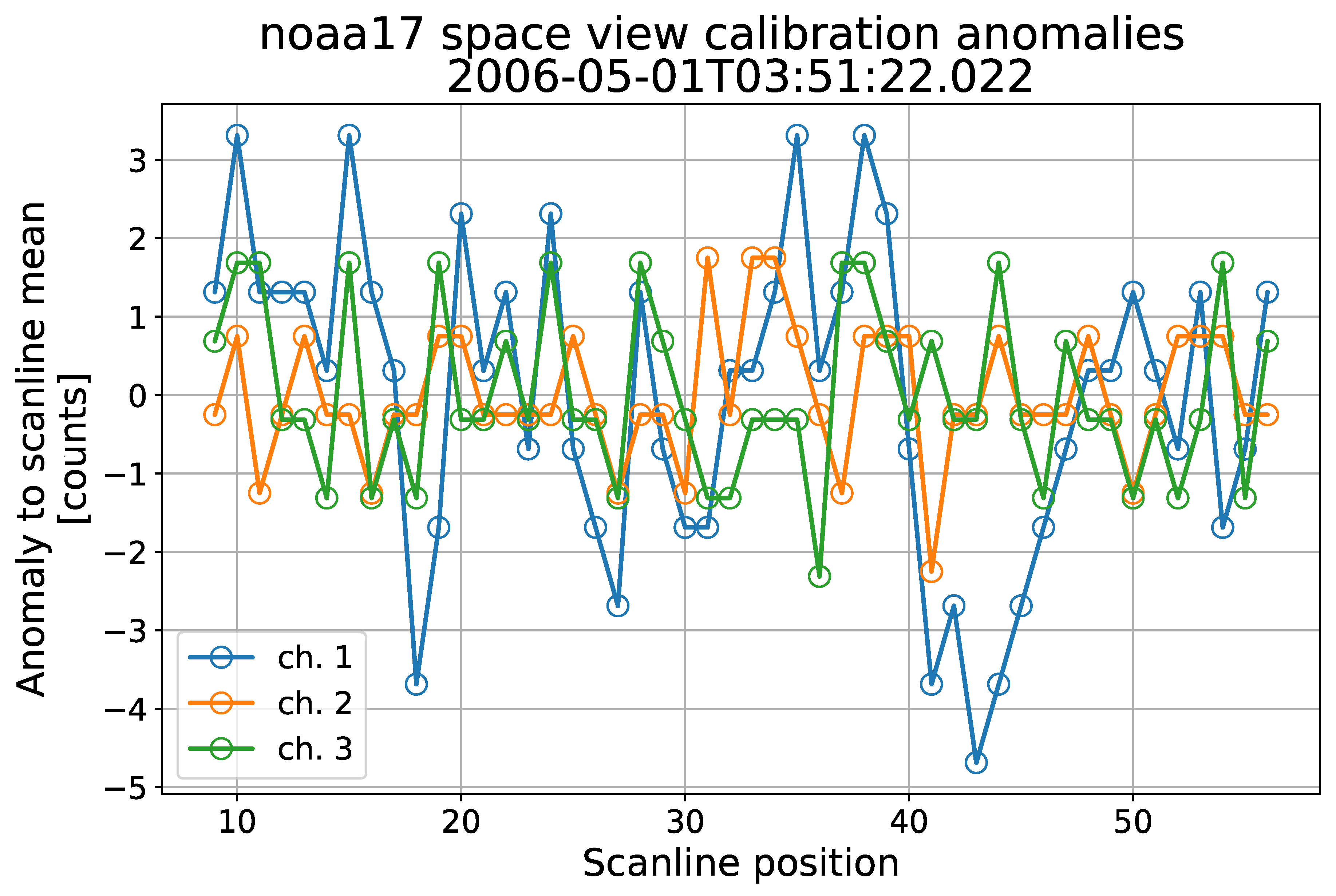
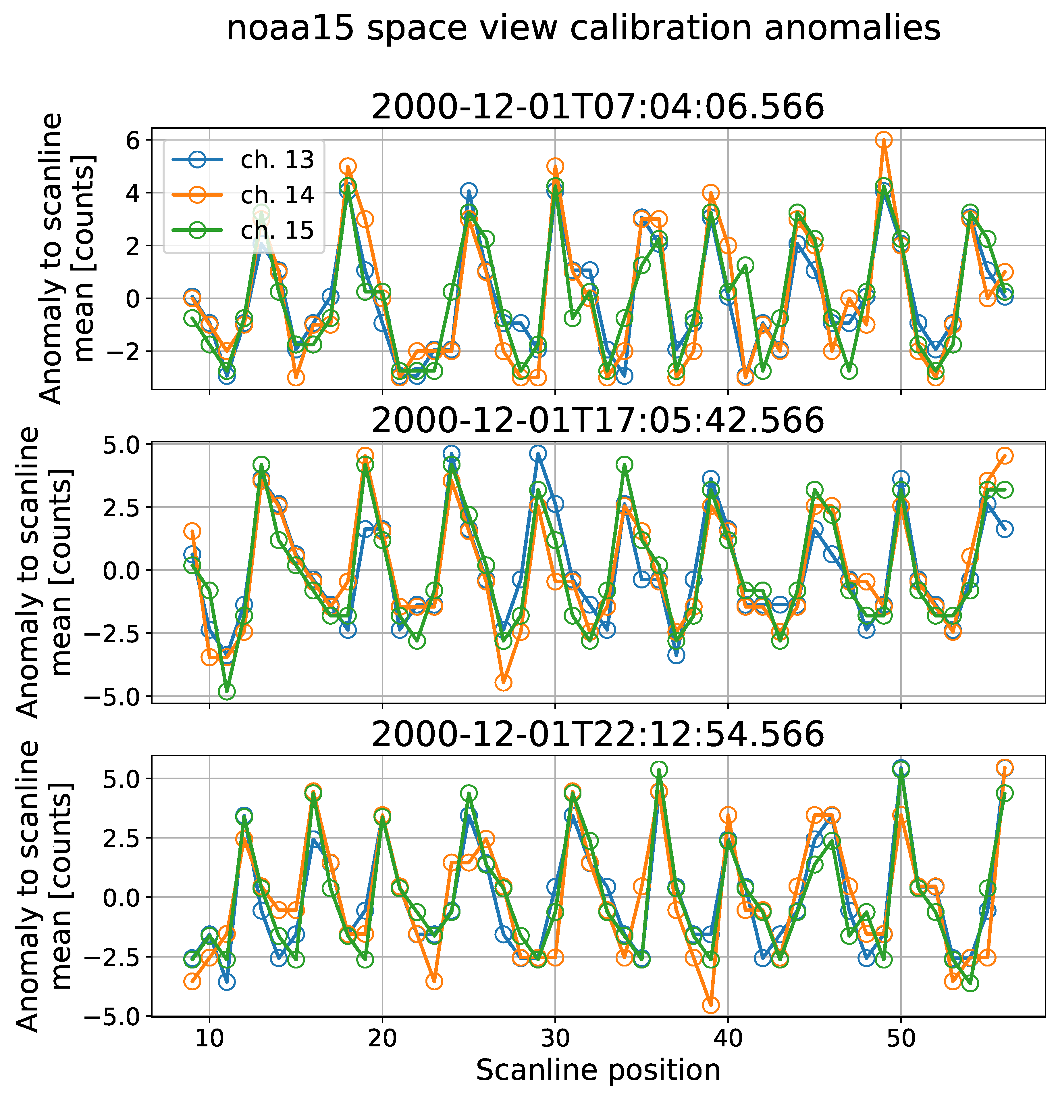
In reality, we observe that space view count deviations (see Equation (1)) may be uncorrelated (as expected), exhibit strong positive correlation, or even exhibit significant negative correlation. For example, Figure 1 shows a case where space view correlations are absent. It shows deviations for channels 6–8 for a single set of calibration measurements on NOAA-14. In contrast, Figure 2 shows an example of strong positive space view count deviations, in this case for channels 13–15 for three sets of calibration measurements on NOAA-15. Two features are immediately apparent from the figure: firstly, the deviations for the three channels are very highly correlated. Therefore, the deviations cannot be caused by white noise, but must be dominated by a shared physical mechanism. Since the measurements for different channels are not taken simultaneously, that mechanism must have some temporal persistence. That brings us to the second feature: the source causing the deviations is quasi-periodic with a period of around 0.5 s. Finally, Figure 3 shows an example where correlations are negative, apparently due to periodic error affecting both channels, but lagging by half a phase in channel 11 compared to channel 10. Negative correlations are less common than positive, but are not exceptional in the HIRS record.

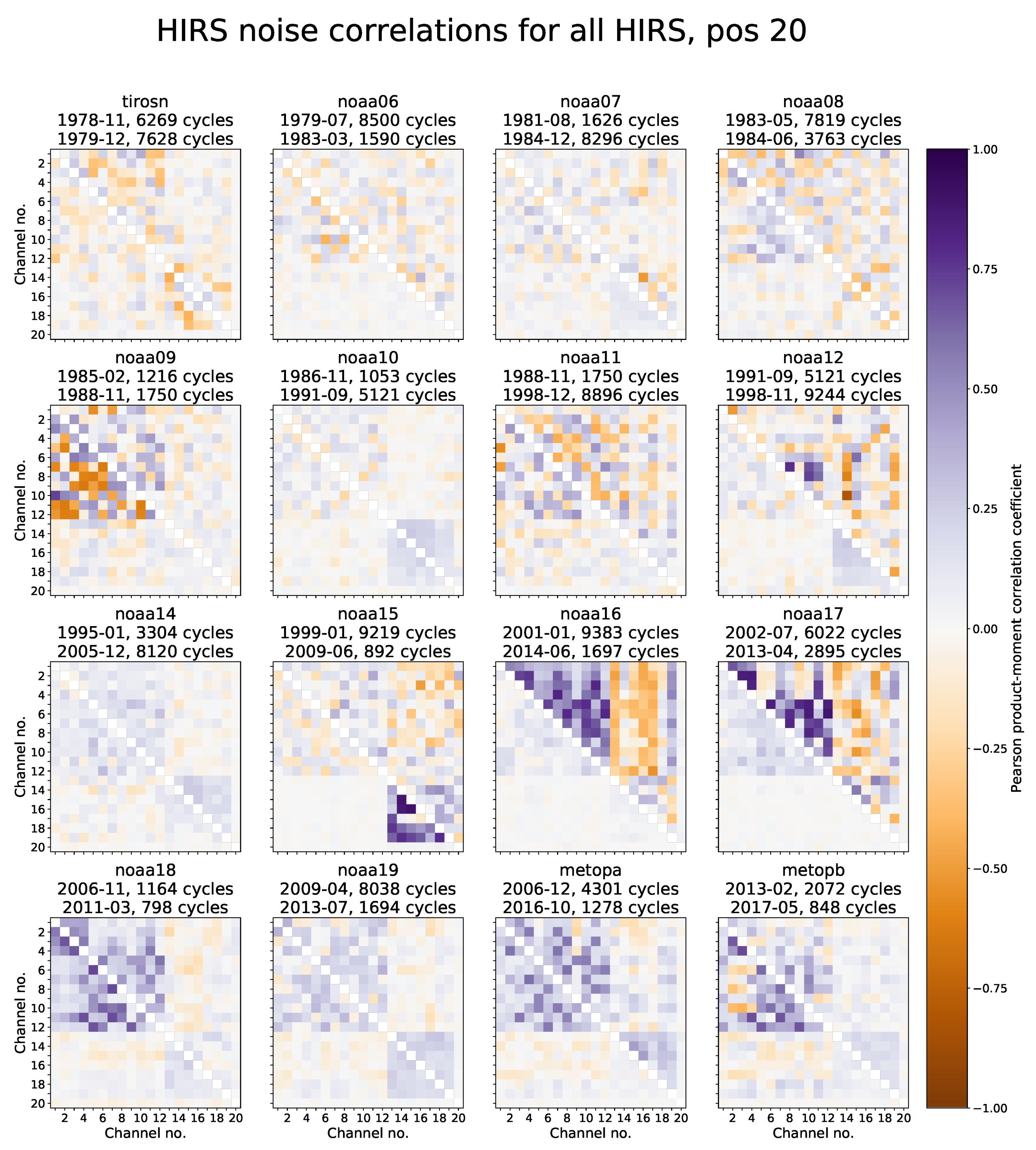
To describe more compactly for what satellites and channel pairs correlations of either sign occur, we calculate the Pearson product-moment correlation according to Equation (2). To account for possible time variations, we do so both early and late within each satellites lifetime. Figure 4 shows the correlations between the error of 20 channels for each instrument on HIRS, for one month early and one month late in each sensor’s lifetime (the diagonal is set to zero, as a reminder that this is not a normal correlation matrix, that there is no information here, and to clearly visually separate the two relevant triangles). This is an evaluation of Equation (2) with v referring to space views, view $b=20$ (chosen arbitrarily), and the number of sets of calibration views according to the numbers shown above each panel. The number of views varies due to data availability and filtering. Note that, for all sensors, there are strong correlations between channels using the same detector and at the same radial distance from the filter wheel central axis, as can be seen by the blocks corresponding to channels 1–12 (HgCdTe detector, smaller radial distance on filter wheel) and 13–19 (InSb detector, larger radial distance on filter wheel). Most sensors have error correlations between channels with different detectors as well, apart from channel 20 (visible, Si detector) where the error is mostly uncorrelated with error in other channels, except during September 2009 for NOAA-15. Correlations can be both positive or negative. Note that an absence of a correlation can either mean that there really is no correlation, or that periods of positive and negative correlation cancel out over the period considered. In many cases (e.g., NOAA-16), correlations within the same detector (and radial distance on filter wheel) are mostly positive, while correlations between channels for different detectors (and different radial distances on filter wheel) take both signs.

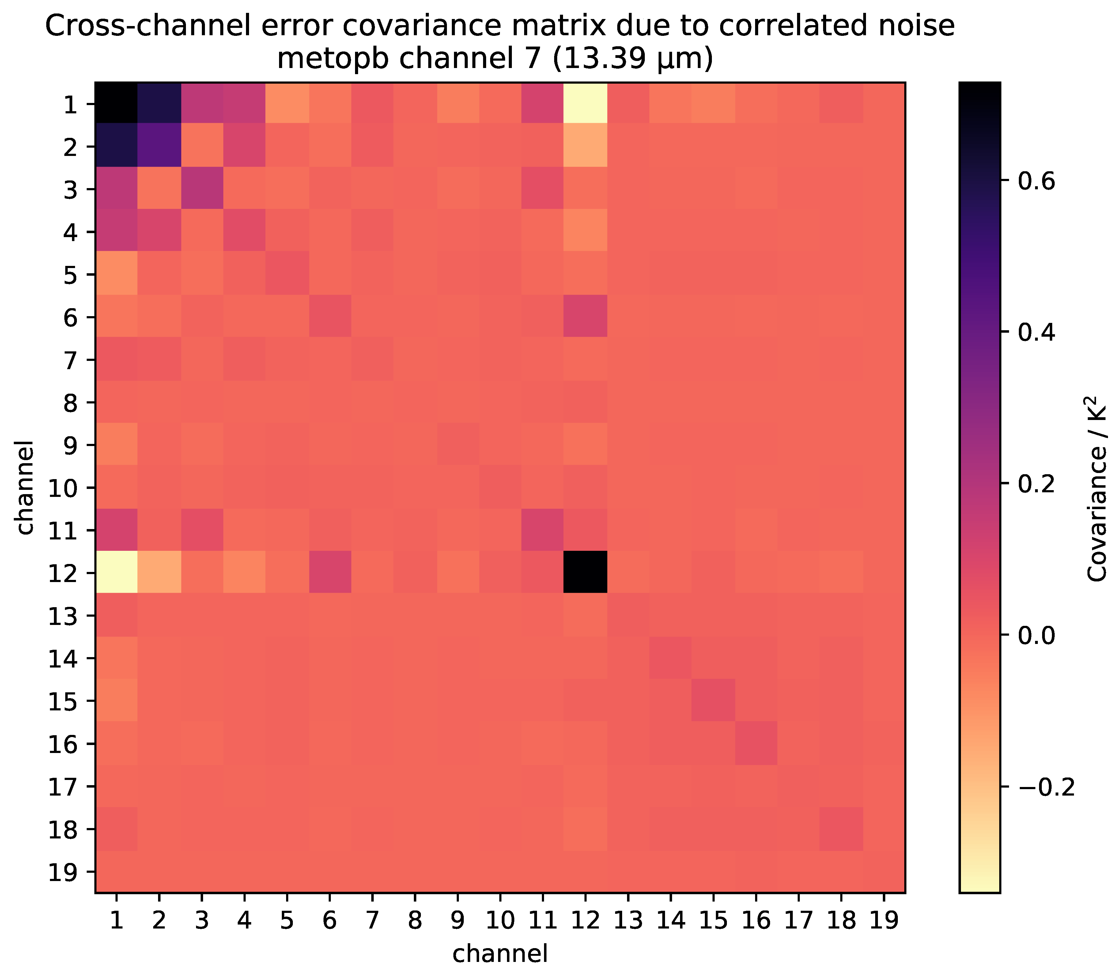
To illustrate how such correlations may propagate to covariances, Figure 5 shows an error covariance matrix for Metop-B channel 7, calculated over a 10 min period on 27 February 2016. This is a variation of a figure published in [9], which explains the mathematics on calculating covariances from correlations using uncertainties and sensitivity coefficients. The figure is less illustrative than correlation matrices, because the scale is dominated by channels with high radiometric noise, but covariances are more directly applicable in many applications.

For some sensors, the error correlations exhibit a strong temporal evolution. This evolution is most prominently visible in the KLM series (NOAA-15, -16, and -17). In the beginning of those sensors, channel errors were uncorrelated between channels with different detectors. For NOAA-17 shortwave (InSb) channels 13–19, errors were initially not correlated at all, a phenomenon otherwise only seen (less clearly) in early NOAA-16 and early NOAA-6 measurements. For each of the KLM series, measurements taken late in the mission lifetime exhibit strong and mostly negative error correlations between channels with different detectors, and NOAA-16 and -17 HgCdTe error correlations become some of the strongest seen in any HIRS at any time. NOAA-15 InSb error correlations however start out strongly positively at the start of the mission, but are more moderate near the end. Other sensors with a clear temporal evolution are NOAA-6 and -7 (inter-detector and InSb), NOAA-8 (inter-detector), NOAA-9 (HgCdTe), and NOAA-12 (inter-detector). The behaviour in recent sensors (NOAA-18 onward) appears more stable, although the error correlation in Metop-A and -B increases somewhat for the InSb detector (channels 13–19), and in MetOp-B decreases somewhat for the HgCdTe detector (channels 1–12).

To take a closer look at such temporal evolution, Figure 6 shows the noise and error correlation behaviour for NOAA-15 HIRS channel 1 for four days in June 1999, as determined by the 2-sample Allan deviation [21],

$$\sigma =\sqrt{\frac{1}{2(N-1)}{\displaystyle \sum _{i=1}^{N-1}}{(y_{i+1}-y_i)}^2},$$

(5)

where $N=48$ for 48 calibration views and $y_i$ is the ith calibration view. The figure shows considerable variability within the space counts—which are between −840 and −820, except on 22 June, when they are between −820 and −800. Several hours into 22 June, the noise level increases from ∼2 counts to ∼4 counts, although with some variability. Around the same time, the nature of the inter-channel correlations changes completely. Prior to 22 June, channel 1 error is strongly positively correlated with error on channel 7, uncorrelated with errors on channels 2 and 5, and negatively correlated with errors on channels 3, 4, and 6. On and after 22 June, channel 1 error is positively correlated with channels 5 and 6, uncorrelated with channels 2, 3, and 4, and negatively correlated with channel 7. This illustrates that the error correlation characteristics change not only on long timescales, but also rapidly on occasion. Inspecting those correlation coefficients over longer timescales (not shown) reveals this particular change in behaviour lasts for more than a week, and that the instrument does not revert to the pre-22 June characteristics. A timeseries for all of 1999 is available on figshare [22]. Similar time-dependent correlation changes occur for other satellites and channels.

3.2. Periodic Error

Figure 2 shows not only a strong correlation, but also a strong periodicity. To take a closer look at such periodicities, we calculate the correlations between different space view anomalies, again for early and late periods for each satellite.

An example is shown in Figure 7, which shows the Pearson product-moment correlation between the error of 48 space views on longwave channel 9 (9.71 μm), using the HgCdTe detector (see Equation (3)). Note that the number of valid views per satellite and month here may differ from the ones in Figure 4, because calculating inter-channel correlations requires all channels to have valid measurements, whereas calculating inter-position correlations for a particular channel only requires that channel to have valid measurements. The figure shows that the periodicity in counts error illustrated in Figure 2 is prominent in many satellites, namely those cases where regular diagonal striping is evident. For Channel 9 on NOAA-6, -7, -10, and -14, view error correlation appears weak or absent. However, if there is periodic error for which the period or phase changes within the time for which the correlation matrices were calculated, the effects may average out. Therefore, absence of evidence in Figure 7 does not imply evidence of absence of periodic error. In NOAA-12, -15, and -17, there is little to no evidence for correlation at the beginning of the mission, but marked correlation is present toward the end. On TIROS-N; NOAA-8, -9, -11, and -16; and MetOp-B, both periods show correlations, but period and magnitude vary. NOAA-18 and -19, and MetOp-A show similar behaviour for both periods shown. Other longwave channels show similar behaviour (not shown).

A shortwave version is shown in Figure 8, which is similar to Figure 7, but for channel 15, a shortwave channel (4.67 μm) using the InSb detector. The correlation patterns are mostly different than for the longwave channels on the HgCdTe detector, although in most cases this difference is in magnitude only. The pattern is different between the channels for TIROS-N, and NOAA-6, -7, -9, -16, and -18.

3.3. Fourier Analysis

We calculate the power spectra (Equation (4)) for space, IWCT, and Earth views. This allows us to compare the magnitude of the periodic error to the magnitude of natural variability in the Earth atmosphere, and determine if the Earth views should be expected to be significantly affected by periodic error.

Figure 9 shows such mean power spectra for a selection of satellites and channels. The selection is a non-representative sample of the 304 satellite/channel-combinations (16 satellites times 19 channels), selected to illustrate the wide range of patterns. The following paragraphs describe the behaviour both in the samples shown, and in the other satellite/channel combinations not shown.

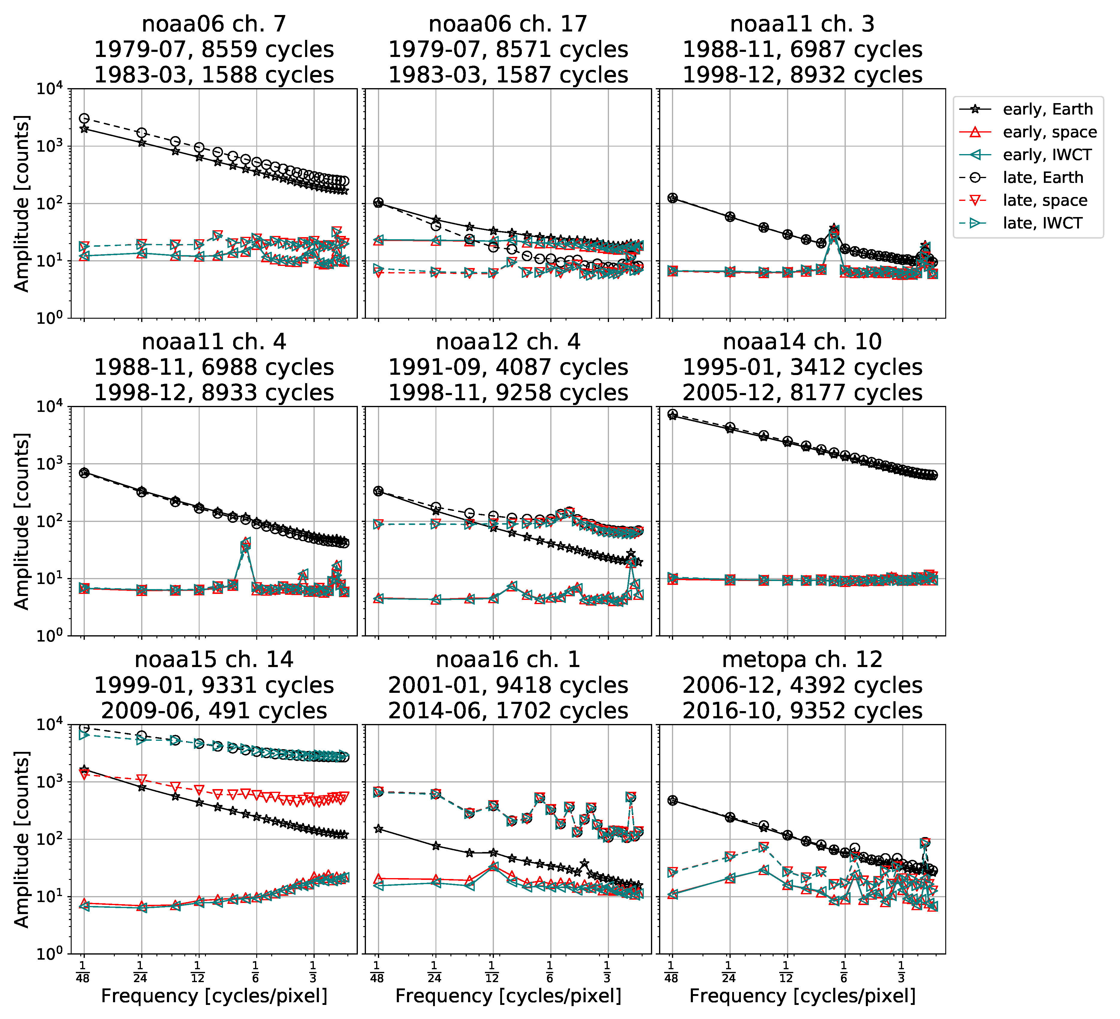
In all satellites, we can see the Fourier spectrum of Earth views (black lines with stars or circles), which follows a power law distribution with a negative slope. That simply means that the variability between two Earth viewing pixels is larger as the distance is increased, which should be expected. Models have previously shown that linear transects of Earth’s surface temperature exhibit a power law [20]. We see similar behaviour in all channels, whether they are surface sensing, temperature sounding, or humidity sounding, with the lines being roughly parallel between the different satellite/sensor pairs shown.

In some cases, the power for the Earth views is stronger near the end of the satellite lifetime (dashed lines) than near the beginning (solid lines). In Figure 9, this is visible for NOAA-6 channel 7, NOAA-12 channel 4, NOAA-15 channel 14, and NOAA-16 channel 1. Where the power in the Earth views in not larger than the power in the calibration views, this may additionally lead to a change in the slope of the Earth views, such as shown for NOAA-6 channel 17, NOAA-12 channel 4, and NOAA-15 channel 14. In those cases, changes in the Earth view power spectrum can be seen along with changes in the calibration view power spectrum, which shows that those changes are instrumental in nature. Some other channels on NOAA-6, -12, and -15 (not shown) show similar behaviour. For all other satellites, the power in the Earth counts spectrum is similar between the beginning and end. We comment more on situations where the power in the Earth views is not larger than the power in the calibration views below.

The red and teal lines with triangles show the mean power spectra for space and IWCT views, respectively. In most cases, the mean power spectra for space and IWCT are (nearly) identical, with the notable exception of NOAA-15 late in its lifetime (channel 14 shown, other channels not shown exhibit similar behaviour). The shape and magnitude of those mean power spectra is very similar for channels sharing the same detector. For all satellites apart from NOAA-10 (not shown) and NOAA-14 (channel 10 shown), the mean power spectrum changes over the lifetime of the satellite. In the absence of any periodic error, one would expect this spectrum to correspond to white noise, which has a constant power as a function of frequency, or 1/f-noise, with a power spectral density decreasing proportionally with 1/f. For some instruments, in particular NOAA-10, NOAA-14, and MetOp-B (not shown), for the longwave channels sharing the HgCdTe detector, noise appears white. However, in other cases, the periodic error is clearly visible in the space and IWCT spectra, e.g., Figure 9 shows for NOAA-11 channels 3 and 4, NOAA-12 channel 4, and MetOp-A channel 12.

Table 3. Summary of notable features in calibration power spectra as shown by the red and teal lines in Figure 9 and similar figures (not shown), for HIRS/2 and HIRS/3 ¹.

	HgCdTe		InSb
	Early	Late	Early	Late
TN	Peak at 9.6 pixels in all except 6, 9, 11.	Broad peak at 6.9–9.6 pixels.	Strong peak at 2.3 pixels. Peaks at 3.4, 4.3, and 9.6 pixels.
N6	Peak at 2.3 and 6 pixels. Weak peak at 9.6 pixels in channels 7 and 10.	Peak at 2.3 pixels only.	Weak peak at 3.4 pixels for all except 17.	Amplitude decreased by factor of approximately 3. Peak at 2.3 pixels. Strong peak at 3.4 pixels for all except 17. Weak peak at 9.6 pixels.
N7	Weak peak at 2.3 pixels. Weak peak at 6 pixels, channels 1–3, 5, 6.	Weak peak at 2.3 pixels. Weak peak at 6 pixels, channels 1–3, 5, 6. Weak peak at 16 pixels in channels 1–6	Mostly flat, weak peak at 3.4 pixels in channels 14, 15, 17.	Peak at 2.1 pixels. Peak at 2.5 pixels. Broad peak at 3.4–4 pixels. Peak at 6.9 pixels, strength varies per channel. Peak at 16 pixels.
N8	Peak at 2.5 pixels. Peak at 3.2 pixels (channel 1 only).	Peak at 2.2 pixels. Weak peak at 3–3.2 pixels (channels 6 and 10). Peak at 6 pixels. Weak peak at 24 pixels.	Peak at 2.3 pixels. Peak at 3.4 pixels (except channel 14). Peak at 4.8 pixels. Peak at 6.9 pixels.	Peak at 2.3 pixels. Peak at 3.4 pixels (except channel 14). Peak at 4.4 pixels. Peak at 6.9 pixels. Weak peak at 24 pixels.
N9	Very strong peak at 4 pixels. Peak at 12 pixels.	Weak peak at 3 pixels. Very strong peak at 4 pixels. Broad peak at 12–16 pixels.	Weak peak at 4 pixels (except channel 17).	Weak peak at 12 pixels, a bit stronger in space than in IWCT.
N10	Weak peaks at 2–3 pixels and broad peak at 6.9 pixels (channels 1–7, 11–12). Weak, broad peak near 3 pixels (channels 8–10).		Weak, broad peak at 3 pixels in channel 19. Otherwise mostly flat.
N11	Peak at 2.3 pixels, strength varies per channel. Peak at 3.7 pixels (channels 2, 4–6). Strong peak at 6.9 pixels.	As for early, except that peak at 3.7 pixels has disappeared.	Peak at 2.3 pixels (channels 13–17). Peak at 6.9 pixels. Peak at 9.6 pixels (channels 14–17).	As for early, but with a weaker peak at 6.9 pixels. The peak at 9.6 pixels is now also visible in channel 19.
N12	Peak at 2.4 pixels (channels 1–7). Broad peak at 6.9 pixels (channels 1–7). Varying weak peaks at 2–3 pixels (channels 8–12). Broad peak at 3 pixels stronger for IWCT than space (channel 8 only).	Amplitude increased by factor of approximately 10. Mostly flat between 48 and 4.8 pixels, decreasing amplitude at 4.8–2 pixels.	Mostly flat.	Mostly flat between 48 and 4.8 pixels, decreasing amplitude at 4.8–2 pixels.
N14	Mostly flat.	Mostly flat.	Mostly flat.	Slight variations in channel 16 only.

and

Table 4. As Table 3, but for HIRS/3 and HIRS/4.

	HgCdTe		InSb
	Early	Late	Early	Late
N15	Mostly flat.	Power increased by nearly 3 orders of magnitude. Power decreases with frequency. Power in space stronger than in IWCT, in particular for lower frequencies. Dominates Earth counts for all channels.	Power increases with frequency.	Power increased by 2–3 orders of magnitude. Power decreases with frequency. Power in space stronger than in IWCT, especially for channels 14 and 18, but not for channel 19.
N16	Weak peak at 12 pixels	Several peaks at 2–7 pixels. Peak at 2.3 pixels particularly strong in channel 9.	Weak peak at 9.6 pixels in channels 13–16, otherwise flat.	Amplitude increased by factor 2–3. Peaks very similar to HgCdTe channels.
N17	Weak peak at 2.8 pixels, channel 10 only, otherwise flat.	Amplitude increased by factor 5–10. Strong peak at 2.3 pixels, affects Earth for all except channel 8. Broad peaks at 4.8 and at 12 pixels.	Flat.	Peaks as for HgCdTe but less strong.
N18	Peak at 3.7 pixels, stronger in IWCT than space. Peak at 2.3 pixels.	Mostly flat, slight increase at highest frequencies.	Weak peaks at 2.3, 2.7, and 9.6 pixels
N19	Weak ups and downs throughout range.	As early data, but with peak at 2.3 pixels varying per strength	Flat.	Peak at 2.3 pixels.
MA	Oscillatory with peaks at 2.3, 3.2, 5.3 pixels.		Flat.	Peaks at 2.3, 6.3, 16 pixels.
MB	Peak at 4 pixels, broad peaks at 4.8–5.3 and at 12–16 pixels	Strong peak at 2.3 pixels, peaks at 5.3 pixels and 3.7–4 pixels.	Flat	Flat

summarise the notable features for the space and IWCT spectra for all HIRS channels on all satellites and channels, including those not shown in the paper. The table is mostly provided for information; a listing in the table does not mean that a satellite/channel should not be used. Although all features tell us something about the workings of the instrument and may impact calibration uncertainty, in some cases the power spectrum of the calibration counts exceeds the expected Earth power spectrum. Essentially, this means that, whatever dominates the calibration power spectrum—whether it is white noise or non-white noise or another form of error (including periodic error)—is also there during Earth views, and is at a particular frequency as strong as or stronger than the Earth signal. This is particularly severe in the case of channel 1, sounding stratospheric temperature. In this channel, all high-frequency and most low-frequency variations are instrumental artefacts. NOAA-7, NOAA-8 and NOAA-16 channel 1 all exhibit a 4-pixel variation in Earth views that is not apparent in space or IWCT views, illustrating that there are sources of periodic error that affect Earth but not calibration counts (it is not due to top of the atmosphere radiation, or it would appear in HIRS measurements on every satellite). In Figure 9, this is visible as a small peak in the early Earth spectrum.

3.4. Effect on Earth Views

For most users of HIRS data, the most important situation is when the power of the IWCT and space error—which is completely instrumental—approaches or exceeds the power of the signal from the Earth views. This may either happen when the data have dominant white noise, or when a strong periodic effect is present in both calibration and Earth views. The cases where periodic error affect the Earth views are:

• TIROS-N: channels 15–17, with a period of 2.3 pixels (frequency of 1/2.3 pixels), and 16–17, period of 4.3 pixels
• Late NOAA-6: channels 15–16, period of 3.4 pixels
• Early NOAA-8: channels 1–3, period of 2.5 pixels
• NOAA-9: channels 4–6, 11, 12, period of 4 pixels
• NOAA-10: channels 2–3, period of 2.5 pixels
• NOAA-11: channels 1–3 at a period of 6.9 pixels, channel 2 at a period of 3.9 pixels, channels 1–3 at a period of 2.3 pixels
• early NOAA-12: channels 2–3, period of 2.4 pixels
• Late NOAA-16: channels 1–6, 9, 11–12 at a period of 2.3 pixels
• Late NOAA-17: channels 1–7, 9–12 at a period of 2.3 pixels
• Late NOAA-19: channels 1–4, 11-12 at a period of 2.3 pixels
• Late MetOp-A: channels 1–4 at a period of 2.3 pixels and 1–3 at a period of 5.3 pixels
• Late MetOp-B: channels 1–4, 12 at a period of 2.3 pixels

4. Discussion and Conclusions

The observed phenomena can broadly be classified into two categories that may or may not be related: error correlations between channels, and periodic error. In some cases, we see both, in other cases only one of those, in yet other cases neither. It is difficult to determine the physical origins of the observed behaviour purely from in-flight data. The diversity of the observed behaviour across different satellites and channels suggests multiple physical causes may be relevant to various members of the HIRS series.

Retrievals of geophysical variables often involve a characterisation of error correlations between measurement vectors, or explicit or implicit assumptions about such error correlations [7]. Typically, instrument errors are assumed to be uncorrelated between channels. Cross-channel error correlation reduces the information content of multi-channel observations, and can be expected to degrade the quality of atmospheric soundings derived from HIRS data where they are present. Moreover, performing a retrieval with the wrong a priori covariance matrix will lead to a retrieval with an incorrect a posteriori covariance matrix. Future work will quantify such implications.

Where the periodic error is adequately predictable, it may be possible to correct for it (leaving some residual errors). Since there are space, IWCT, and possibly ICCT views every 40 scanlines, a correction model could be frequently updated. This may enhance significantly the utility of HIRS data in situations where such correlated error affects Earth views. Such a correction is recommended for future work.

The study reported here is part of the production of a new harmonised FCDR to cover all HIRS measurements between 1982 and 2016. The FIDUCEO HIRS FCDR will contain metrologically traceable uncertainty information per datum, including detailed information on correlation structures per orbit. It will include information on inter-channel correlations (such as illustrated in Figure 5, inter-scanline correlations, and inter-view correlations, in the form described by Merchant et al. [9]. Spectral analysis or quality flags related to periodic error will not be directly included in the upcoming FCDR, but it will contain information in each orbit file (such as calibration counts in an easy to read form) to aid in its further study. HIRS has the potential for long-term climate studies, but only with metrologically traceable uncertainties and sensor-to-sensor harmonisation, including correlation information such as presented in this study. The reader can find more information on FIDUCEO, including access to FCDRs upon their publication, at http://www.fiduceo.eu/.

References

- Koenig, E.W. Final Report on the High Resolution Infrared Radiation Sounder (HIRS) for the Nimbus F Spacecraft; Technical Report; ITT Aerospace/Optical Division: Fort Wayne, IN, USA, 1975. [Google Scholar]
- English, S.J.; Renshaw, R.J.; Dibben, P.C.; Smith, A.J.; Rayer, P.J.; Poulsen, C.; Saunders, F.W.; Eyre, J.R. A comparison of the impact of TOVS and ATOVS satellite sounding data on the accuracy of numerical weather forecasts. Q. J. R. Meteorol. Soc. 2000, 126, 2911–2931. [Google Scholar]
- Dee, D.P.; Uppala, S.M.; Simmons, A.J.; Berrisford, P.; Poli, P.; Kobayashi, S.; Andrae, U.; Balmaseda, M.A.; Balsamo, G.; Bauer, P.; et al. The ERA-Interim reanalysis: Configuration and performance of the data assimilation system. Q. J. R. Meteorol. Soc. 2011, 137, 553–597. [Google Scholar] [CrossRef]
- Bates, J.J.; Jackson, D.L. Trends in upper-tropospheric humidity. Geophys. Res. Lett. 2001, 28, 1695–1698. [Google Scholar] [CrossRef]
- Shi, L.; Bates, J.J. Three decades of intersatellite-calibrated High-Resolution Infrared Radiation Sounder upper tropospheric water vapor. J. Geophys. Res. 2011, 116. [Google Scholar] [CrossRef]
- Wylie, D.P.; Menzel, W.P.; Strabala, K.I. Four years of global cirrus cloud statistics using HIRS. J. Clim. 1994, 7, 1972–1986. [Google Scholar]
- Rodgers, C.D. (Ed.) Inverse Methods for Atmospheric Sounding: Theory and Practice; World Scientific Publishing: Singapore, 2000; ISBN 10981022740X. [Google Scholar]
- Mittaz, J.; Merchant, C.J.; Wooliams, E. Applying principles of metrology to historical Earth observations from satellites. Metrologia 2019, in press. [Google Scholar] [CrossRef]
- Merchant, C.J.; Holl, G.; Mittaz, J.P.; Wooliams, E.R. Radiance uncertainty characterisation to facilitate Climate Data Record creation. Remote Sens. 2019, 11, 474. [Google Scholar] [CrossRef]
- Cao, C.; Jarva, K.; Ciren, P. An Improved Algorithm for the Operational Calibration of the High-Resolutino Infrared Radiation Sounder. J. Atmos. Ocean. Technol. 2007, 24, 169–181. [Google Scholar] [CrossRef]
- Shi, L.; Bates, J.J.; Cao, C. Scene radiance-dependent intersatellite biases of HIRS longwave channels. J. Atmos. Ocean. Technol. 2008, 25, 2219–2229. [Google Scholar] [CrossRef]
- Shi, L. Intersatellite Differences of HIRS Longwave Channels between NOAA-14 and NOAA-15 and between NOAA-17 and METOP-A. IEEE Trans. Geosci. Remote 2013, 51, 1414–1424. [Google Scholar] [CrossRef]
- Chen, R.; Cao, C.; Menzel, W.P. Intersatellite calibration of NOAA HIRS CO2 channels for climate studies. J. Geophys. Res. 2013, 118, 5190–5203. [Google Scholar] [CrossRef]
- Menzel, W.P.; Frey, R.A.; Borbas, E.E.; Baum, B.A.; Cureton, G.; Bearson, N. Reprocessing of HIRS Satellite Measurements from 1980 to 2015: Development toward a Consistent Decadal Cloud Record. J. Appl. Meteorol. Clim. 2016, 55, 2397–2410. [Google Scholar] [CrossRef]
- Gierens, K.; Eleftheratos, K.; Sausen, R. Intercalibration between HIRS/2 and HIRS/3 channel 12 based on physical considerations. Atmos. Meas. Tech. 2018, 11, 939–948. [Google Scholar] [CrossRef] [Green Version]
- Robel, J.; Graumann, A.; Kidwell, K.; Aleman, R.; Goodrum, G.; Mo, T.; Ruff, I.; Askew, J.; Graumann, A.; Muckle, B.; et al. NOAA KLM User’s Guide with NOAA-N, -N’ Supplement; Technical Report; National Oceanic and Atmospheric Administration, National Environmental Satellite, Data, and Information Service, National Climatic Data Center, Remote Sensing and Applications Division: Silver Spring, MD, USA, 2014.
- Kidwell, K.B. NOAA Polar Orbiter Data User’s Guide; Technical Report; National Oceanic and Atmospheric Administration: Asheville, NC, USA, 1997.
- Pearson, K. Notes on regression and inheritance in the case of two parents. Proc. R. Soc. Lond. 1895, 58, 240–242. [Google Scholar]
- Fourier, J.B.J. Mémoire sur les Temperature du Global Terrestre et de Espace Planétaires. Mémoire de l’Académie Royale des Sciences de l’Institut de France 1827, 7, 570–604. [Google Scholar]
- Fallah, B.; Saberi, A.A.; Sodoudi, S. Emergence of global scaling behaviour in the coupled Earth-atmosphere interaction. Sci. Rep. 2016, 6, 34005. [Google Scholar] [CrossRef] [PubMed]
- Allan, D.W. Statistics of atomic frequency standards. Proc. IEEE 1966, 54, 221–230. [Google Scholar] [CrossRef]
- Holl, G.; Mittaz, J.; Merchant, C.J. Timeseries of noise characteristics and instrument error correlations for the High Resolution Infrared Radiation Sounder on the NOAA-15 satellite. Figshare 2017. [Google Scholar] [CrossRef]
- Walt, S.V.D.; Colbert, S.C.; Varoquaux, G. The NumPy array: A structure for efficient numerical computation. Comput. Sci. Eng. 2011, 13, 22–30. [Google Scholar] [CrossRef]
- Jones, E.; Oliphant, T.; Peterson, P. SciPy: Open source scientific tools for Python. 2001. [Google Scholar]
- Hunter, J.D. Matplotlib: A 2D graphics environment. Comput. Sci. Eng. 2007, 9, 90–95. [Google Scholar] [CrossRef]
Figure 1.
Example of space view deviations for one set of calibration measurements for channels 6–8 on NOAA-14. The date and time for the measurements are shown in the figure title.
Figure 2.
Like Figure 1, but showing three examples for channels 13–15 on NOAA-15.
Figure 3.
Example of space view deviations for three sets of calibration measurements for two channels on NOAA-9.
Figure 4.
Pearson product-moment correlation between the error in different channels for all HIRS satellites. The lower triangles show correlations during a month early in the sensor life, whereas the upper triangles show the same, but late in the sensor life. Those triangles do not include the diagonal, which includes no information and is indicated as zero, as a reminder that this is not a normal correlation matrix. The title for each panel indicates the number of sets of calibration measurements ( in Equation (2)) used to calculate the correlation coefficients, and the month illustrated in the data.
Figure 5.
Illustration of covariance matrix for Metop-B channel 7, calculated during 17:39:37–17:49:45 on 27 February 2016.
Figure 6.
Noise and error correlation behaviour for four days of NOAA-15 channel 1 in June 1999: (top) all individual counts for the space views for each set of calibration measurements (48 per set), along with a histogram; (middle) the two-sample Allan deviation for each set and a corresponding histogram; and (bottom) a time series of the error correlation coefficient for noise between channel 1 and six other channels (2–7).
Figure 7.
Pearson product-moment correlation between the error at different views within a set of calibration measurements (labelled “pos no”), channel 9, for the IWCT view. The lower triangle refers to a month early in the lifetime of each instrument, whereas the upper triangle refers to a month late in its lifetime, each indicated in the title above each panel.
Figure 8.
Like Figure 7, but for channel 15.
Figure 9.
Time-averaged power spectrum of calibration cycles and Earth views for a selection of satellites and months. The duration of a pixel is 0.1 s, so a peak near cycles/pixel corresponds to periodic error with a period of 0.6 s. Each panel shows the average power spectrum during an early month for the satellite and channel (solid lines with stars and triangles pointing up or left) and a month during a late month for the satellite (dashed lines with circles and triangles pointing down or right). Earth views are in black with stars or circle, space views are in red with up- or down-pointing triangles, and IWCT views are in teal with left- or right-pointing triangles. In most cases, Earth and IWCT views have the same mean power spectrum so their lines are indistinguishable. The text above each panel indicates the corresponding satellite, channel, period, and the number of sets of calibration measurements used to calculate the power spectrum. Note that for any particular panel, the number of sets of Earth views is a factor 37 (HIRS/2, HIRS/2I) or 38 (HIRS/3, HIRS/4) higher than the number of sets of calibration views.