Object-Based Land Cover Classification of Cork Oak Woodlands using UAV Imagery and Orfeo ToolBox

Abstract

This paper investigates the reliability of free and open-source algorithms used in the geographical object-based image classification (GEOBIA) of very high resolution (VHR) imagery surveyed by unmanned aerial vehicles (UAVs). UAV surveys were carried out in a cork oak woodland located in central Portugal at two different periods of the year (spring and summer). Segmentation and classification algorithms were implemented in the Orfeo ToolBox (OTB) configured in the QGIS environment for the GEOBIA process. Image segmentation was carried out using the Large-Scale Mean-Shift (LSMS) algorithm, while classification was performed by the means of two supervised classifiers, random forest (RF) and support vector machines (SVM), both of which are based on a machine learning approach. The original, informative content of the surveyed imagery, consisting of three radiometric bands (red, green, and NIR), was combined to obtain the normalized difference vegetation index (NDVI) and the digital surface model (DSM). The adopted methodology resulted in a classification with higher accuracy that is suitable for a structurally complex Mediterranean forest ecosystem such as cork oak woodlands, which are characterized by the presence of shrubs and herbs in the understory as well as tree shadows. To improve segmentation, which significantly affects the subsequent classification phase, several tests were performed using different values of the range radius and minimum region size parameters. Moreover, the consistent selection of training polygons proved to be critical to improving the results of both the RF and SVM classifiers. For both spring and summer imagery, the validation of the obtained results shows a very high accuracy level for both the SVM and RF classifiers, with kappa coefficient values ranging from 0.928 to 0.973 for RF and from 0.847 to 0.935 for SVM. Furthermore, the land cover class with the highest accuracy for both classifiers and for both flights was cork oak, which occupies the largest part of the study area. This study shows the reliability of fixed-wing UAV imagery for forest monitoring. The study also evidences the importance of planning UAV flights at solar noon to significantly reduce the shadows of trees in the obtained imagery, which is critical for classifying open forest ecosystems such as cork oak woodlands.

1. Introduction

Cork oak woodlands characterize forested Mediterranean landscapes, and their ecological and economic values are largely recognized, although not adequately valorized [1]. This ecosystem covers about 2.2 million hectares across the globe, but the most extensive groves are located on the Atlantic coast of the Iberian Peninsula, to the extent that Portugal and Spain produce 75% of the world’s cork [2]. Cork is the sixth-most important non-wood forest product globally, and it is used to produce wine stoppers and a wide variety of other products, including flooring components, insulation and industrial materials, and traditional crafts. The most frequent landscape in the Mediterranean region is characterized by open woodland systems in which scattered mature trees coexist with an understory composed of grassland for livestock or cereal crops and shrubs. The ecosystem has high conservation value and provides a broad range of goods and services besides cork [2]. It is important to increase the knowledge and skills that enable the use of the most innovative technologies to monitor these forest ecosystems in the support of forest management.

The use of unmanned aerial vehicles (UAVs) or UA systems (UASs) in forest and environmental monitoring [3,4,5,6,7,8,9,10,11,12,13,14,15] is currently in an expansion phase, encouraged by the constant development of new models and sensors [3,16,17]. Detailed reviews focusing on the use of UAVs in agro-forestry monitoring, inventorying, and mapping are provided by Tang and Shao [16], Pádua et al. [3], and Torresan et al. [18]. Additionally, the short time required for launching a UAV mission makes it possible to perform high-intensity surveys in a timely manner [16,19,20], thus granting forest practices with more precision and efficiency while opening up new perspectives in forest parameter evaluation. Therefore, UAVs are particularly suitable for multi-temporal analysis of small- and medium-sized land parcels and complex ecosystems, for which frequent surveys are required [17].

There is a large diversity of UAV applications, mainly as a result of the variety of available sensors [21]. The most common sensors assembled on UAVs are passive sensors, which include classic RGB (red, green, blue) cameras, NIR (near-infrared), SWIR (short-wave infrared), MIR (mid-infrared), TIR (thermal infrared), and their combinations in multispectral (MS) and hyperspectral (HS) cameras and active sensors such as RADAR (radio detection and ranging) and LiDAR (laser imaging detection and ranging) [3,16]. An increasingly common agro-forestry application that uses multispectral images acquired from sensors assembled on UAVs is land cover classification [18,22].

Until a decade ago, most of the classification methods for agro-forestry environments were based on the statistical analysis of each separate pixel (i.e., pixel-based method), and performed well when applied to satellite imagery covering large areas [23,24,25]. The recent emergence of very high resolution (VHR) images, which are becoming increasingly available and cheaper to acquire, has introduced a new set of possibilities for classifying land cover types at finer levels of spatial detail. Indeed, VHR images frequently show high intra-class spectral variability [19,20,26]. On the other hand, the higher spatial resolution of these images enhances the ability to focus on an image’s structure and background information, which describe the association between the values of adjacent pixels. With this approach, spectral information and image classification are largely improved [27].

Recently, object-based image analysis (OBIA) has emerged as a new paradigm for managing spectral variability, and it has replaced the pixel-based approach [27,28]. OBIA works with groups of homogeneous and contiguous pixels [19] (i.e., geographical objects, also known as segments) as base units to perform a classification, so it differs from the classic pixel-oriented methods that classify each pixel separately; thus, the segmentation approach reduces the intra-class spectral variability caused by crown textures, gaps, and shadows [19,27,28]. OBIA includes two main steps: (i) identification, grouping, and extraction of significant homogeneous objects from the input imagery (i.e., segmentation); (ii) labeling and assigning each segment to the target cover class (classification) [19,20,28].

More recently, considering that OBIA techniques are applied in many research fields, when referring to a geospatial context, the use of GEOBIA (geographic OBIA) [27,29,30] has become the preferred method. Moreover, GEOBIA should be considered as a sub-discipline of GIScience, which is devoted to obtaining geographic information from RS imagery analysis [27,29,30]. GEOBIA has proven to be successful and often superior to the traditional pixel-based method for the analysis of very high resolution UAV data, which exhibits a large amount of shadow, low spectral information, and a low signal-to-noise ratio [6,19,20,26].

The availability of hundreds of spectral, spatial, and contextual features for each image object can make the determination of optimal features a time-consuming and subjective process [20]. Therefore, high radiometric and geometric resolution data require the simultaneous use of more advanced and improved computer software and hardware solutions [26]. Several works dealing with the classification of forest ecosystems or forest tree species by coupling GEOBIA and UAV imagery can be found in the literature [4,15,16,22,31]. Franklin and Ahmed [31] reported the difficulty in performing an accurate tree crown reconstruction, characterizing fine-scale heterogeneity or texture, and achieving operational species-level classification accuracy with low or limited radiometric control. Deciduous tree species are typically more difficult to segment into coherent tree crowns than evergreens [31] and tend to be classified with lower accuracies [32].

In terms of using GEOBIA algorithms, most studies are implemented by means of proprietary software (e.g., [4,6,11,15,19,31]). Considering their cost, especially in an operational context, it can be argued that only a relatively restricted group of operators can use them. Nowadays, several free and open-source software packages for geospatial (FOSS4G) analysis with GEOBIA algorithms are available, thus making their use accessible to a larger number of end users [20]. Among others, a very promising FOSS4G package equipped with GEOBIA algorithms is Orfeo ToolBox (OTB), developed by the French Centre National d’Etudes Spatiales (CNES). OTB can be operated either autonomously or through a second open-source software (i.e., QGIS), used as a graphical interface that enables a graphical analysis of data processing in real time [33,34].

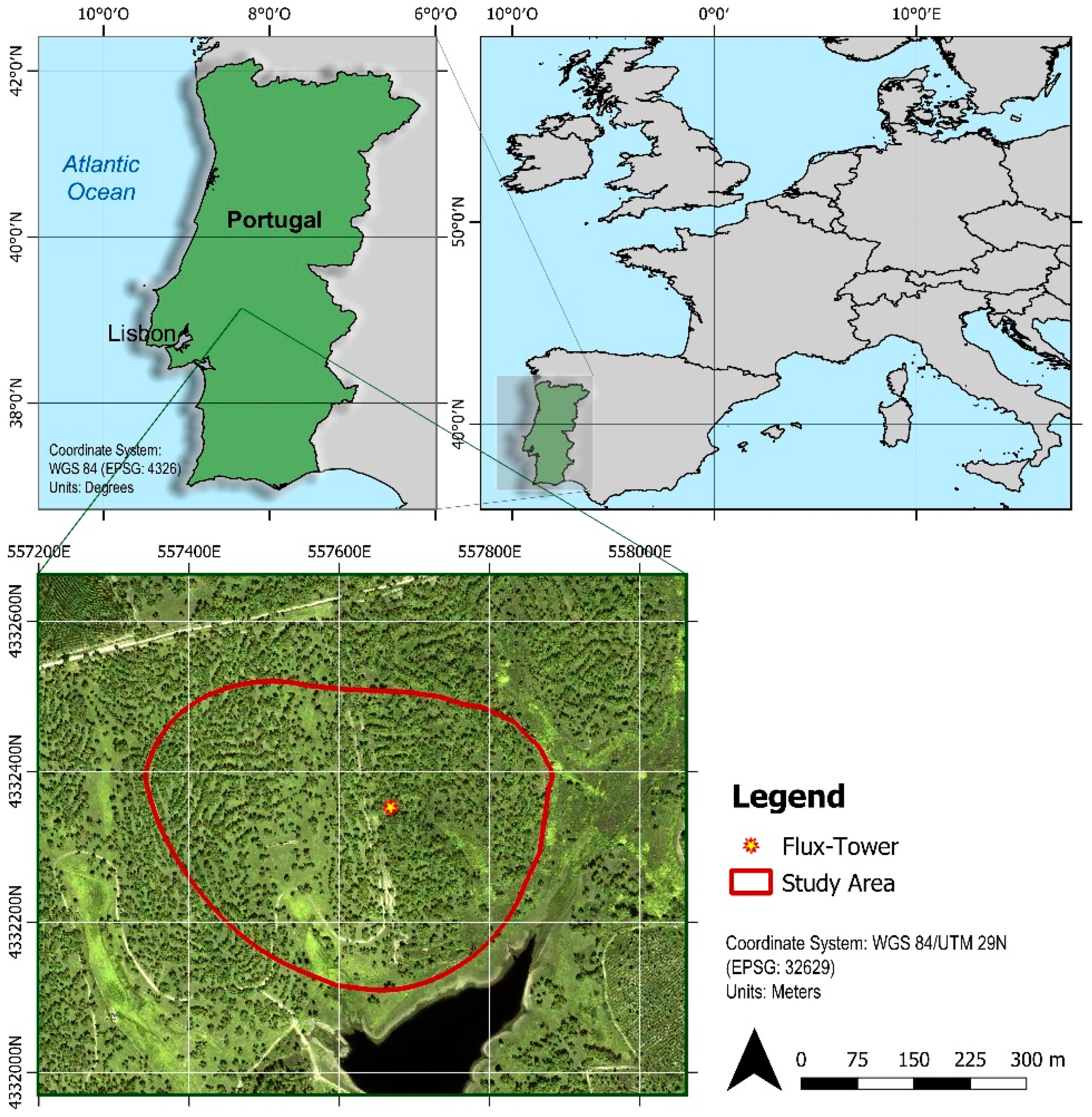
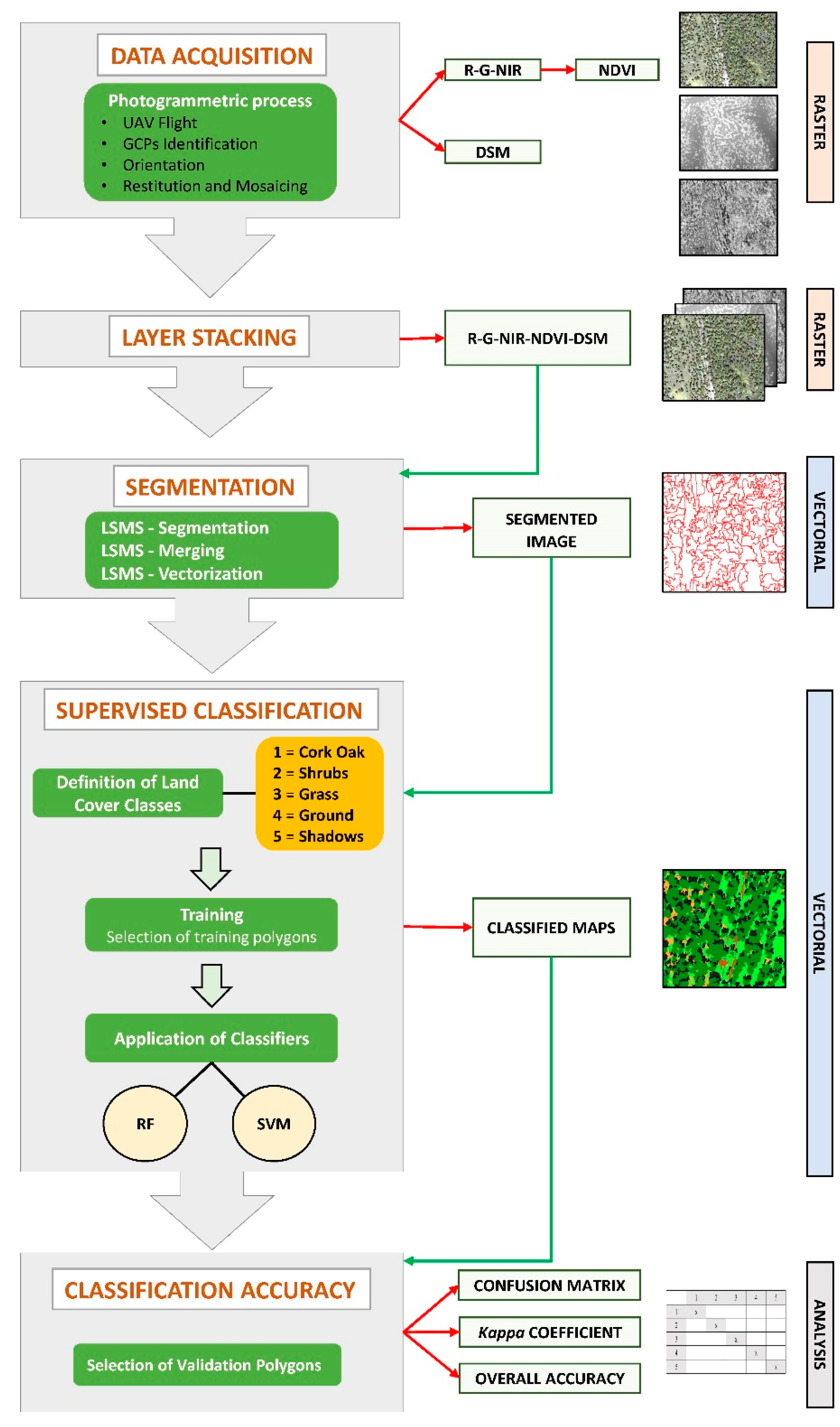
This work was conducted in the framework of a wider project aiming to derive a methodology for monitoring the gross primary productivity (GPP) of Mediterranean cork oak (Quercus suber L.) woodland by integrating spectral data and biophysical modeling. The spatial partition of the ecosystem into different coexisting vegetation layers (trees, shrubs, and grass), which is the task encompassed by this study, is essential to the fulfillment of the objective of the overarching project. The main objective of this work was to develop a supervised classification procedure of the three vegetation layers in a Mediterranean cork oak woodland by applying a GEOBIA workflow to VHR UAV imagery. In order to optimize the procedure, two different algorithms were compared: support vector machine (SVM) and random forest (RF). In addition, data from two contrasting surveying periods—spring and summer—were also compared in order to assess the effect of the composition of different layers (i.e., no living grass in the summer period) on the classification accuracy. In order to increase the processing quality, we tested a methodology based on the combination of spectral and semantic information to improve the classification procedure through the combined use of three informative layers: R-G-NIR mosaics, NDVI (normalized difference vegetation index), and DSM (digital surface model).

The paper is organized as follows. Section 2 provides details about the study area and the dataset, and gives a general description of OTB. Section 3 deals with methodological issues by explaining preprocessing, segmentation, classification methods and tools, and the performed accuracy analyses. In Section 4, the obtained results are shown, and they are discussed in Section 5. Section 6 summarizes the results and highlights the limitations of the present research, open questions, and suggested future research directions.

2. Materials

2.1. Study Area

The study area is located in Central Portugal (39º08’ N; 08º19’ W) and covered by a Mediterranean cork oak woodland (Figure 1). The climate is typically Mediterranean with hot and dry summers, while most of the precipitation is concentrated between autumn and early spring (from October to April). Quercus suber is the only tree species present, and the understory is composed of a mixture of shrubs and herbaceous species [35]. The shrubby layer is composed primarily of two species, Cistus salvifolius and Ulex airensis, while the herbaceous layer is dominated by C3 species, mainly grasses and legumes. The site is a permanent research infrastructure where carbon, water, and energy are regularly measured by eddy covariance [36]. The study area is delimited by the 70% isoline of the flux tower footprint—an estimate of the extent and position of the surface contributing to the fluxes [37].

2.2. Dataset

2.2.1 Data Acquisition

We used a fixed-wing UAV (SpinWorks S20; Figure 2) with a wingspan of 1.8 m and a modified RGB camera with a radiometric resolution of 8 bit per channel in which the blue channel was replaced by an NIR channel. The main characteristics of the S20 are summarized in

Table 1. Technical characteristics of the S20 unmanned aerial vehicle (UAV) and the onboard camera [38], and features of the two flights (spring and summer).

Technical Characteristics of S20
Maximum take-off weight	2.0 kg
Maximum weight of the payload (sensors)	0.4 kg
Maximum flight autonomy	2 h
Cruising speed	60 km h−1
Maximum operating range drone- pilot station	20 km
productivity (hectares per hour)	200 ha h−1
Bands	Red, Green, NIR
Pixel resolution	12.1 Mpx
Size of the sensor	7.6 × 5.7 mm
Field of view	73.7 × 53.1 degrees
Focus	24 mm
Ground sample distance (GSD)	5 cm pixel−1 at 100 m of flight height
Features of the two flights
Covered area	100 hectares
Flight height	100 m
Sidelap and overlap	60% and 90%
N° of photos	1500
Duration of flights	41 min (spring), 28 min (summer)

, while further descriptive details can be found in Soares et al. [38]. Flight planning (Figure 2) was carried out using the ground station software integrated with the S20 system that was developed by the SpinWorks company [38].

2.2.2 Flight Data Processing and Outputs

Photogrammetric and image processing procedures were carried out and are synthetically depicted in the workflow (Figure 3). In this procedure, each image taken in-flight has the geographical position and elevation logged using the navigation system and the onboard computer. With this information, the raw dataset is processed using a structure-from-motion (SFM) technique during which the identification of common features in overlapping images is carried out. Subsequently, a 3D point cloud is generated from which a digital surface model (DSM) is interpolated, which in turn is used to orthorectify each image. Finally, all of these images are stitched together in an orthomosaic. Two orthomosaics were derived from two flights that were carried out in different seasons of 2017: spring (5 April at 13:00) and summer (13 July at 11:00) (

Table A1. Meteorological conditions characterizing the two flights (spring and summer).

Date	UTC Zone	Reference Time	Takeoff LT	Landing LT	Flight Duration (minutes)	Wind Conditions	Sun Elevation (deg)	Sun Azimuth (deg)
05-04-2017	UTC+1	13:00	12:37	13:18	41	Strong	56.14	163.81
13-07-2017	UTC+1	11:00	10:49	11:17	28	Light	51.97	105.33

). Moreover, each orthomosaic was radiometrically corrected in post-processing using a calibrated reflectance panel imaged before and after each of the flights. The use of the same scene in two different periods allowed for testing the classification algorithm’s capacity to take into account the differences caused by variation in the phenological status as it changed throughout the various biological cycles of the main plant species. The resultant mosaics have an extension of 100 ha (a square of 1000 × 1000 m) and a resampled GSD (ground sample distance) of 10 cm.

2.3. ORFEO ToolBox (OTB)

OTB is an open-source project for processing remotely sensed imagery, developed in France by CNES (www.orfeo-toolbox.org, accessed 10 April 2019) [39]. It is a toolkit of libraries for image analysis and is freely accessible and manageable by other open-source software packages as well as command-line [33,34,40]. The algorithms implemented in OTB were applied in this work through the QGIS software (www.qgis.org, accessed 10 April 2019). The OTB version used was 6.4.0; it interfaced with QGIS 2.18 Las Palmas, which was installed on an outdated workstation (

Table A2. Main technical specification of the workstation used for data processing.

Model	Dell Precision Workstation T7500
Processor	Intel Xeon CPU E5503 @ 2.00 GHz, 1995 MHz, 2 Kernels, 2 Logical Processors
RAM installed	6.00 GB
System Type	x64-based PC

). This is an important detail that highlights the fluidity of OTB because it works even with underperforming hardware. In OTB, the algorithms used in the phase of image object analysis were Large-Scale Mean-Shift (LSMS) segmentation for the image segmentation, and SVM and RF for the object-based supervised classification.

3. Methods

The implemented workflow can be simplified into four main steps: preprocessing, segmentation, classification, and accuracy assessments (Figure 3).

3.1. Preprocessing

For both the spring and summer flights, a DSM with a GSD of 10 cm was derived for its usefulness in further classification stages since trees, shrubs, and grass have very different heights. For every informative layer used in the next stage of classification, and therefore for every input layer, a linear band stretching (rescale) to a range at 8 bits, from 0 (minimum) to 255 (maximum), was performed. The aim of this process, as described in Immitzer et al. [41], was to normalize each band to a common range of values in order to reduce the effect of potential outliers on the segmentation. Subsequently, for both raster files (spring and summer) containing the R-G-NIR bands, a layer stacking process was performed by merging NDVI and DSM data to obtain two final five-band orthomosaics. This step was necessary because OTB segmentation procedure requires a single raster image as input data. Successively, a window of the original scene was made so that only a smaller area of interest, corresponding to the footprint of the flux tower, was classified (approximately 16.85 ha).

3.2. Spectral Separability

In order to measure the separability of the NDVI and the DSM layers of different types of vegetation present in the study area (cork oak, shrubs, and grass) and, consequently, their importance for the classification provided by the original spectral bands (R-G-NIR), we implemented the M-statistic, defined originally by Kaufman and Remer and modified as follows:

$$M=\frac{|{\mu }_1-{\mu }_2|}{({\sigma }_1+{\sigma }_{2)}}$$

(1)

where μ₁ is the mean value for class 1, μ₂ is the mean value for class 2, σ₁ is the standard deviation for class 1, and σ₁ is the standard deviation for class 2. M-statistic expresses the difference in μ (the signal) normalized by the sum of their σ (that can be interpreted as the noise) (i.e., the separation between two samples by class distribution). Larger σ values lead to more overlap of the two considered bands, and therefore to less separability. If M < 1, classes significantly overlap and the ability to separate (i.e., to discriminate) the regions is poor, while if M > 1, class means are well separated and the regions are relatively easy to discriminate.

3.3. Segmentation

Segmentation is the first phase of the object-oriented classification procedure, and its result is a vector file in which every polygon represents an object. Original images are subdivided into a set of objects (or segments) that are spatially adjacent, composed of a set of pixels with homogeneity or semantic meaning, and collectively cover the whole image. The shape of every notable object should be ideally represented by one real object in the image [19,27]. Segmentation focuses not only on the radiometric information of the pixels, but also on the semantic properties of each segment, on the image structure, and on other background information (color, intensity, texture, weft, shape, context, dimensional relations, and position) whose values describe the association between adjacent pixels.

The Large-Scale Mean-Shift (LSMS)-segmentation algorithm is a non-parametric and iterative clustering method that was introduced in 1975 by Fukunaga and Hostetler [42]. It enables the performance of tile-wise segmentation of large VHR imagery, and the result is an artifact-free vector file in which each polygon corresponds to a segmented image containing the radiometric mean and variance of each band [33,34]. This method allows for the optimal use of the memory and processors, and was designed specifically for large-sized VHR images [42]. The OTB LSMS-segmentation procedure is composed of four successive steps [33,34]:

• LSMS-smoothing;
• LSMS-segmentation;
• LSMS-merging;
• LSMS-vectorization.

In the first phase, we tested the reliability of LSMS-smoothing in the segmentation process by adopting different values of the spatial radius (i.e., the maximum distance to build the neighborhood from averaging the analyzed pixels [35]). Starting from the default value of the spatial radius (5), we tested the following values: 5–10, 15, 20, and 30. However, considering that LSMS-smoothing did not improve the results of the segmentation process and is an optional step, we omitted it. Thus, we started from the second step (LSMS-segmentation).

For this step, the literature was reviewed to make an informed choice of the values of the different parameters. However, all examined publications focus on the urban field and the use of satellite imagery. This highlights the lack of previous application of the method to the classification of plant species from UAV imagery. Thus, several tests were completed to assess different values of the range radius, defined as the threshold of the spectral signature distance among features and expressed in radiometry units [34,35]. This parameter is based on the Euclidean distance among the spectral signature’s values of pixels (spectral difference). Therefore, the range radius will have at least the same value of the minimum difference to discriminate these two pixels as two different objects. First, we measured the Euclidean distance of spectral signatures in several regions of interest, with particular attention given to cork oak. After that, we tested numerous values around the recorded minimum spectral distances (i.e., all values between 5 and 30 with steps of 1 unit).

Given the segmentation result, the third step dealt with merging small objects with larger adjacent ones with the closest radiometry. The minsize (minimum size region) parameter enables the specification of the threshold for the size (in pixel) of the regions to be merged. If, after the segmentation, a segment’s size is lower than this criterion, the segment is merged with the segment that has the closest spectral signature [33,34]. For this parameter, we measured a number of smaller cork oak crowns so as to determine a suitable threshold value (Figure A1).

The last step is LSMS-vectorization, in which the segmented image is converted into a vector file that contains one polygon per segment.

3.4. Classification and Accuracy Assessment

The classification was implemented for five land cover classes: cork oak, shrubs, grass, soil, an shadows. There are several object-oriented classification machine learning algorithms implemented in OTB, both unsupervised and supervised (e.g., RF, SVM, normal Bayes, decision tree, k-nearest neighbors). In our case, two supervised methods were tested: RF and SVM. These commonly used classifiers, as also specified in Li et al. [43] and Ma et al. [25], were deemed to be the most suitable supervised classifiers for GEOBIA because their classification performance was excellent. In supervised algorithms, decision rules developed during the training phase are used to associate every segment of the image with one of the preset classes. Supervised classification has become the most commonly used type for the quantitative analysis of remotely sensed images, as the resulting evaluation is found to be more accurate when accurate ground truth data are available for comparison [25,44,45].

3.4.1 Choice and Selection of the Training Polygons

Before the selection of the training polygons, it was important to carry out an on-field exploratory survey of the region under study. After this, for each of the five land cover classes, 150–350 polygons were selected from each of the two five-band orthomosaics. These training polygons were manually selected by on-screen interpretation while taking into consideration a good distribution among the five land cover classes and the different chromatic shades characterizing the study area. As explained by Congalton and Green [46], to obtain a statistically consistent representation of the analyzed image, the accuracy assessment requires that an adequate number of samples should be collected per each land cover class. To this end, we considered it appropriate to select a total number of trainer polygons that did not deviate from 2% of the total number of segments of the entire image (5.48% and 3.01% in terms of covered surface for spring and summer images, respectively). Regarding the distribution among land cover classes, the number of samples was defined according to the relative importance of that class within the classification objectives.

3.4.2. Implementation of Support Vector Machine (SVM) and Random Forest (RF) Classification Algorithms

SVM is a supervised non-parametric classifier based on statistical learning theory [47,48] and on the kernel method that has been introduced recently for the application of image classification [49]. SVM classifiers have demonstrated their efficacy in several remote sensing applications in forest ecosystems [49,50,51,52].

This classifier aims to build a linear separation rule between objects in a dimensional space (hyperplane) using a φ(·) mapping function derived from training samples. When two classes are nonlinearly separable, the approach uses the kernel method to realize projections of the feature space on higher dimensionality spaces, in which the separation of the classes is linear [33,34]. In their simplest form, SVMs are linear binary classifiers (−1/+1) that assign a certain test sample to a class using one of the two possible labels. Nonetheless, a multiclass classification is possible, and is automatically executed by the algorithm.

Random forest is an automatic learning algorithm introduced by Leo Breiman [53] and improved with the work of Adele Cutler [54]. It consists of a set of decision trees and uses bootstrap aggregation, namely, bagging, in order to create different formation subsets for producing a variety of trees, any one of which provides a classification result. The algorithm classifies the input vector with every single decision tree and returns the classification label, which is the one with the most “votes”. All of the decision trees are trained using the same parameters but on different training sets. The algorithm produces an internal and impartial estimation of the generalization error using so-called out-of-bag (OOB) samples, which contain observations that exist in the original data and do not recur in the bootstrap sample (i.e., the training subset) [54].

The experiences of Trisasongko et al. [55] and Immtzer et al. [41] show that the default values of the OTB parameters for training and classification processes seem to provide optimal results. In view of this, in this study we used default values for both classification algorithms. With SVM, we used a linear kernel-type with a model-type based on a C value equal to 1. For the RF algorithm, the maximum depth of the tree was set to 5, while the maximum number of trees in the forest was fixed to 100. The OOB error was set to 0.01.

3.4.3. Accuracy Assessment

Accuracy assessment was implemented on the basis of systematic sampling through a regular square grid of points with dimensions of 20 × 20 m; the sampling procedure was applicable to the whole study area. After that, we selected all polygons containing the sampling points, and for each of them we compared the ground truth with the predicted vegetation class. Thus, confusion matrices for RF and SVM algorithms were generated. Finally, producer’s and user’s accuracy and the kappa coefficient (Khat) were calculated.

4. Results

4.1. Spectral Separability

The spectral separability allows the ranking of the variables in their ability to discriminate the different land cover classes, and provides an insight of their usefulness in the segmentation and classification procedures. Results show that NDVI plays an important role, being the variable with the highest value of the M-statistic in the summer flight and the second in the spring flight (

Table 2. Spectral separability (M-statistic) provided by red, green, NIR, NDVI, and DSM for both flights (spring and summer). Land cover classes are denoted as follows: 1 = cork oak; 2 = shrubs; 3 = grass. The highest value of the statistic is highlighted for each pair of classes.

Spring
	Red	Green	NIR	NDVI	DSM
M1,2	0.021	2.148	0.004	0.250	1.040
M1,3	0.473	0.700	0.387	0.777	1.199
M2,3	0.494	0.673	0.420	0.450	0.032
Summer
	Red	Green	NIR	NDVI	DSM
M1,2	0.402	0.228	0.487	0.823	0.568
M1,3	0.139	0.308	0.303	2.000	0.739
M2,3	0.306	0.559	0.240	0.75	0.135

). During the summer period, NDVI maximizes the contrast between the evergreen cork oak trees and the senescent herbaceous vegetation. Besides the spectral variables, the separability obtained with the data concerning the vegetation height (DSM) is important to discriminate between trees/shrubs and trees/grass, in particular in the spring flight when the herbaceous layer is green.

4.2. Segmentation

The absence of suitable material in the literature from which to take a cue for the choice of parameter values drastically influenced the testing approach. The attainment of the optimal final values of the parameters of the LSMS-segmentation algorithm was effectively possible only by performing a long series of attempts using small sample areas according to theoretical fundamentals.

Adopting spatial radius values lower than 10 led to results that were similar to those obtained without the smoothing step, while higher values in the smoothing phase worsened the obtained segmentation (Figure 4). Moreover, with values of the spatial radius that were lower than 10, the computation time of the smoothing process was around 10 hours, and it reached around thirty-six hours with a value of 30. Therefore, we decided to eliminate the smoothing step from our final workflow. In the second phase of our tests, we optimized the range radius and the minimum region size. We discarded range radius values lower than 6 because they led to over-segmentation, while values over 7 led to under-segmentation, which is characterized by poor segmentation for cork oak (Figure 4). For the minsize, we adopted a threshold obtained by measuring a number of smaller cork oak crowns (minimum values of about 2.5 m², corresponding to the adopted threshold of 250 pixels).

The evaluation of different combinations of these parameters, and therefore of the obtained segmentations, was performed by means of visual interpretation by superimposing them over the orthomosaic. We obtained the most satisfactory results after setting the range radius value to 7 and the size of tiles to 500 × 500 pixels. These values proved to be the most reliable for both spring and summer imagery. The region merge step followed the segmentation stage, from which 26,815 and 49,575 segments were obtained for the spring and summer flights, respectively. Figure 4 shows a set of examples of the segmentation procedure with the superimposition of the vector file containing segments on the RGB image from a small portion of the study area.

4.3. Classification and Accuracy Assessment

In the training phase, 586 polygons for the spring image and 1067 polygons for the summer image (corresponding to 2.18% and 2.15% of the total number, respectively) were selected. Details on the surface distribution and spectral characteristics of the training and validation polygons according to the five land-use classes are provided in Appendix A (

Table A3. Surface distribution of training and validation polygons according to the five defined land cover classes. Land cover classes are denoted as follows: 1 = cork oak; 2 = shrubs; 3 = grass; 4 = soil; 5 = shadows.

	Trainers		Validation
	Spring	Summer	Spring	Summer
Class	Area [ha]	Area [ha]	Area [ha]	Area [ha]
1	0.1119	0.0963	0.1257	0.05
2	0.0586	0.0891	0.0599	0.01
3	0.6017	0.2095	0.8970	0.490
4	0.0702	0.0258	0.0162	0.022
5	0.0613	0.0759	0.0473	0.032
Number of polygons	586	1067	479	393

and

Table A4. Main statistics (mean = µ, standard deviation = σ, minimum = Min, and maximum = Max) of training polygons in each spectral band according to the five defined land cover classes for both orthomosaics (spring and summer). Land cover classes are denoted as follows: 1 = cork oak; 2 = shrubs; 3 = grass; 4 = soil; 5 = shadows.

SPRING
	Red			Green			NIR			NDVI			DSM
Class	µ ± σ	Min	Max	µ ± σ	Min	Max	µ ± σ	Min	Max	µ ± σ	Min	Max	µ ± σ	Min	Max
1	36.33 ± 8.57	10	64	56.24 ± 14.50	13	112	100.60 ± 17.06	48	149	0.62 ± 0.09	0.02	1	159.19 ± 6.26	141.90	169.72
2	36.67 ± 7.30	13	76	58.97 ± 11.41	19	111	100.72 ± 14.57	52	170	0.57 ± 0.11	0.14	0.94	146.88 ± 5.57	140.95	167.25
3	42.95 ± 5.41	12	86	73.07 ± 9.54	16	184	111.47 ± 10.99	48	178	0.48 ± 0.09	–0.02	1	146.56 ± 4.27	138.97	166.52
4	63.53 ± 10.28	33	102	130.01 ± 25.50	60	224	141.82 ± 15.73	84	197	0.21 ± 0.07	0.01	0.68	150.67 ± 3.99	135.63	160.96
5	17.22 ± 4.84	8	55	25.29 ± 9.76	10	116	60.18± 9.37	45	124	0.58 ± 0.17	−0.012	1	150.88 ± 5.29	137.42	166.39
SUMMER
	Red			Green			NIR			NDVI			DSM
Class	µ ± σ	Min	Max	µ ± σ	Min	Max	µ ± σ	Min	Max	µ ± σ	Min	Max	µ ± σ	Min	Max
1	40.66 ± 8.09	14	69	64.48 ± 13.36	20	112	109.57 ± 16.48	57	169	0.60 ± 0.07	0.17	0.95	157.80 ± 7.27	142.59	167.31
2	34.59 ± 7.01	14	68	58.76 ± 11.67	24	104	94.69 ± 14.05	58	173	0.46 ± 0.10	–0.03	0.85	150.73 ± 5.18	142.18	166.25
3	38.66 ± 6.30	17	69	72.66 ± 13.20	28	139	100.93 ± 11.98	60	165	0.34 ± 0.06	0.02	0.81	149.49 ± 3.97	136.76	166.65
4	68.52 ± 7.28	45	99	145.70 ± 19.13	90	219	148.67 ± 10.86	107	195	0.16 ± 0.06	–0.01	0.55	143.04 ± 5.87	136.04	160.72
5	26.67 ± 6.69	12	59	44.72 ± 13.26	17	123	78.45 ± 12.91	50	136	0.45 ± 0.9	0.04	0.87	150.13 ± 4.12	136.33	165.11

). The two resulting land cover maps are shown in Figure 5 and Figure 6.

The incidence of the cork oak class is almost the same for both classifiers and in both flights, with values ranging between just over 40% for the RF classifier (40.10% spring, 40.31% summer) and nearly 39% for SVM (38.95% spring, 38.58% summer). The shrubs class represents about 10% according to RF in both spring and summer imagery, while for the SVM algorithm, shrubs form about 12% of the classified area. The grass class accounts for about 32.5% of the area (32.83% RF, 32.24% SVM) from the spring flight, while for the summer flight, this value is about 29% (28.95% RF, 29.22% SVM). Shadows cover 15.03% (RF) and 14.91% (SVM) in the spring image, while in the summer image, shadows amount to just over 19% (19.23% RF, 19.47% SVM). The class representing bare soil does not exceed 1.62%.

Table 3. Confusion matrices for both classification algorithms, random forest (RF) and support vector machines (SVM), and for both flights (spring and summer). Land cover classes are denoted as follows: 1 = cork oak; 2 = shrubs; 3 = grass; 4 = soil; 5 = shadows.

RF Spring		Ground Truth					Total	User’s accuracy
		1	2	3	4	5
Classified	1	148	1	3	0	0	152	97.37%
	2	1	104	1	0	0	106	98.11%
	3	0	0	43	2	0	45	95.56%
	4	0	0	0	8	0	8	100%
	5	1	0	1	0	96	98	97.96%
Total		150	105	48	10	96	479
Producer’s accuracy		98.67%	99.05%	89.58%	80%	100%
SVM Spring		Ground Truth					Total	User’s accuracy
		1	2	3	4	5
Classified	1	147	1	2	0	0	150	98%
	2	2	96	7	1	0	106	90.57%
	3	1	8	38	1	0	48	79.17%
	4	0	0	0	8	0	8	100%
	5	0	0	1	0	96	97	98.97%
Total		150	105	48	10	96	479
Producer’s accuracy		98%	91.43%	79.17%	80%	100%
RF Summer		Ground Truth					Total	User’s accuracy
		1	2	3	4	5
Classified	1	155	0	2	0	0	157	98.73%
	2	5	40	2	0	3	50	80.00%
	3	0	0	97	0	1	98	98.98%
	4	0	0	2	5	0	7	71.43%
	5	2	0	3	0	75	80	93.75%
Total		162	40	106	5	79	392
Producer’s accuracy		95.68%	100%	91.51%	100%	94.94%
SVM Summer		Ground Truth					Total	User’s accuracy
		1	2	3	4	5
Classified	1	151	1	3	0	2	157	96.18%
	2	1	33	10	0	6	50	66%
	3	0	1	94	0	3	98	95.92%
	4	0	0	2	5	0	7	71.43%
	5	3	10	1	0	66	80	82.50%
Total		155	45	110	5	77	392
Producer’s accuracy		97.42%	73.33%	85.45%	100%	85.71%

reports the confusion matrices for the accuracy assessment, while

Table 4. Kappa index and overall accuracy for both classification algorithms, random forest (RF) and support vector machine (SVM), and for both flights (spring and summer).

Imagery	Kappa Value	Overall Accuracy
RF Spring	0.973	97.6%
SVM Spring	0.935	94.1%
RF Summer	0.928	94.9%
SVM Summer	0.847	89.0%

reports the kappa values and the overall accuracy for both RF and SVM classification algorithms and for both spring and summer flights. On the basis of 479 and 393 validation polygons for spring and summer flights, respectively, the user’s accuracy for the cork oak class is 97.37% (spring) and 98.73% (summer) for RF, while for SVM it is 98% (spring) and 96.18% (summer). The values of the producer’s accuracy are 98.67% (spring) and 95.68% (summer) for RF, and 98% (spring) and 97.42% (summer) for SVM. For the shrubs class, the user’s accuracy of the RF classifier is between 80% (summer) and about 98% (spring), and for SVM it is about 90% in the spring flight, while it dropped to 66% in the summer flight.

A similar difference is registered for the producer’s accuracy, whose values are close to 100% for RF, while for SVM, they are 91.43% and 73.33% in spring and summer, respectively. The grass class is classified with a user’s accuracy of 95.56% (spring) and 98.98% (summer) for RF and 79.17% (spring) and 95.92% (summer) for SVM.

The producer’s accuracy reaches 89.58% (spring) and 91.51% (summer) with RF, and 79.17% (spring) and 85.45% (summer) for SVM. Table 4 indicates an overall accuracy of 97.6% for RF and 94.1% for SVM in the spring image, with kappa values ranging from 0.973 to 0.935 for RF and SVM, respectively. The overall accuracy for the summer mosaic is 94.9% for RF and 89% for SVM, with kappa values of around 0.928 for RF and 0.847 for SVM.

Both classifiers (RF and SVM) did not require particular computational resources. Both imagery classification steps, including the training phase, took a few seconds (from 1 to 10 seconds; in this computing time, we excluded the selection of trainers that we performed manually).

5. Discussion

5.1. Segmentation

Given that it was expected to worsen the results, the smoothing step of the standard segmentation workflow provided in OTB was omitted because it reduces the contrast necessary to discriminate between the cork oak and shrub classes. The optimization of the range radius and minsize values led to a consistent separation between cork oak, shrubs, and grass classes.

To accomplish the segmentation step with the high structural and compositional heterogeneity of the site, we adopted a low-scale factor of objects, and this was effective. Actually, in the LSMS-segmentation algorithm, the scale factor can be only managed through the adopted values of the range radius and minimum region size parameters. As reported by scholars [56,57,58,59], even today, the visual interpretation of segmentation remains the recommended method to assess the quality of the obtained results.

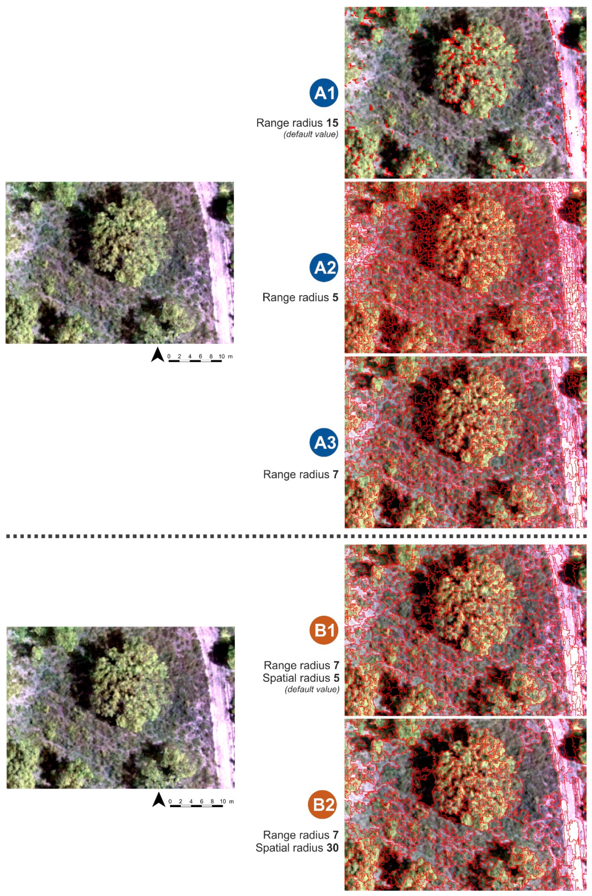
Taking into account the high geometrical resolution of our imagery (i.e., GSD = 10 cm), a low scale of segmentation was preferable; thus, relatively low values of the range radius and minimum region size were used. Even though producing very small segments, in some cases, leads to over-segmentation (i.e., a single semantic feature is split into several segments, which then need to be merged), a low scale of objects effectively resulted in a high degree of accuracy. It allowed the identification of polygons that represent every small radiometric difference in tree crowns, as well as small patches of grass and shrubs (Figure 3). As highlighted in several studies [29,60,61,62], a certain degree of over-segmentation is preferable to under-segmentation to improve the classification accuracy, as can be clearly inferred from the results in Table 3 and Table 4.

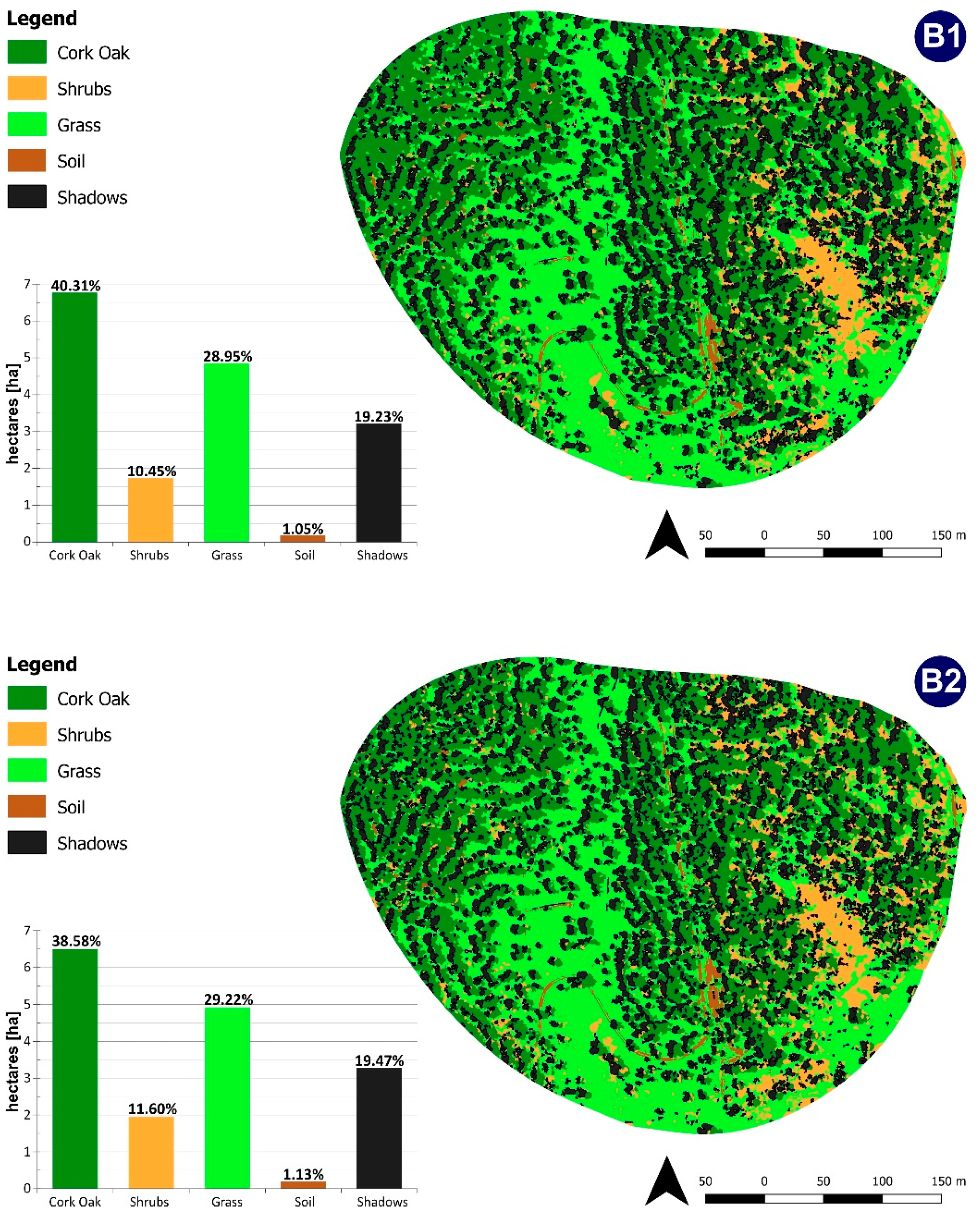
It is important to underline a very significant difference in the number of polygons in the segmentation results of the two different mosaics, despite our application of region merging using the same threshold size (250 pixels). As shown in the results section, the summer image presents almost twice the number of polygons relative to the spring image. This might be explained by a higher chromatic difference caused by a high contrast of vegetation suffering from drought (especially Cistus and the herbaceous layer) and by an increased presence of shadows (an increase of more than 4% of the study area compared with the spring image). Actually, the summer flight was performed earlier in the day (11:00) than the spring one (13:00), so the flights were subjected to different sun elevation angles (Table A1). Nevertheless, Figure 3 shows that the obtained segmentation correctly outlines the boundaries of the tree crowns, as well as the shrub crowns and the surrounding grass spots, discriminating one from the other. The segmentation results also clearly differentiate between the bare soil and the vegetation, even in the presence of small patches. As reported in recent studies that performed forest tree classification [18,59], the additional information provided by the DSM and NDVI significantly improves the delimitation and discrimination of segments, which was true in our case as well. This is more relevant in conditions in which the three vegetation layers are spatially close, because discrimination based only on spectral information has proven very difficult to achieve in such environments. An additional detail to mention is that the algorithm was able to accurately recognize the shadows, an important “disturbing factor” for image processing, since they are usually hardly distinguished from other objects. This is the reason why shadows were specifically considered as a separate class category.

5.2. Classification and Accuracy Assessment

The GEOBIA paradigm coupled with the use of machine learning classification algorithms is currently considered an excellent “first-choice approach” for the classification of forest tree species and the general derivation of forest information [28,31,41,55,63]. As reported by Trisasongko et al. [55] and Immtzer et al. [41] and confirmed in this study, the default values of the OTB parameters for training and classification processes provide optimal results, and they were maintained in the final test. Moreover, both classifiers were very fast, requiring just around 10 seconds for their execution.

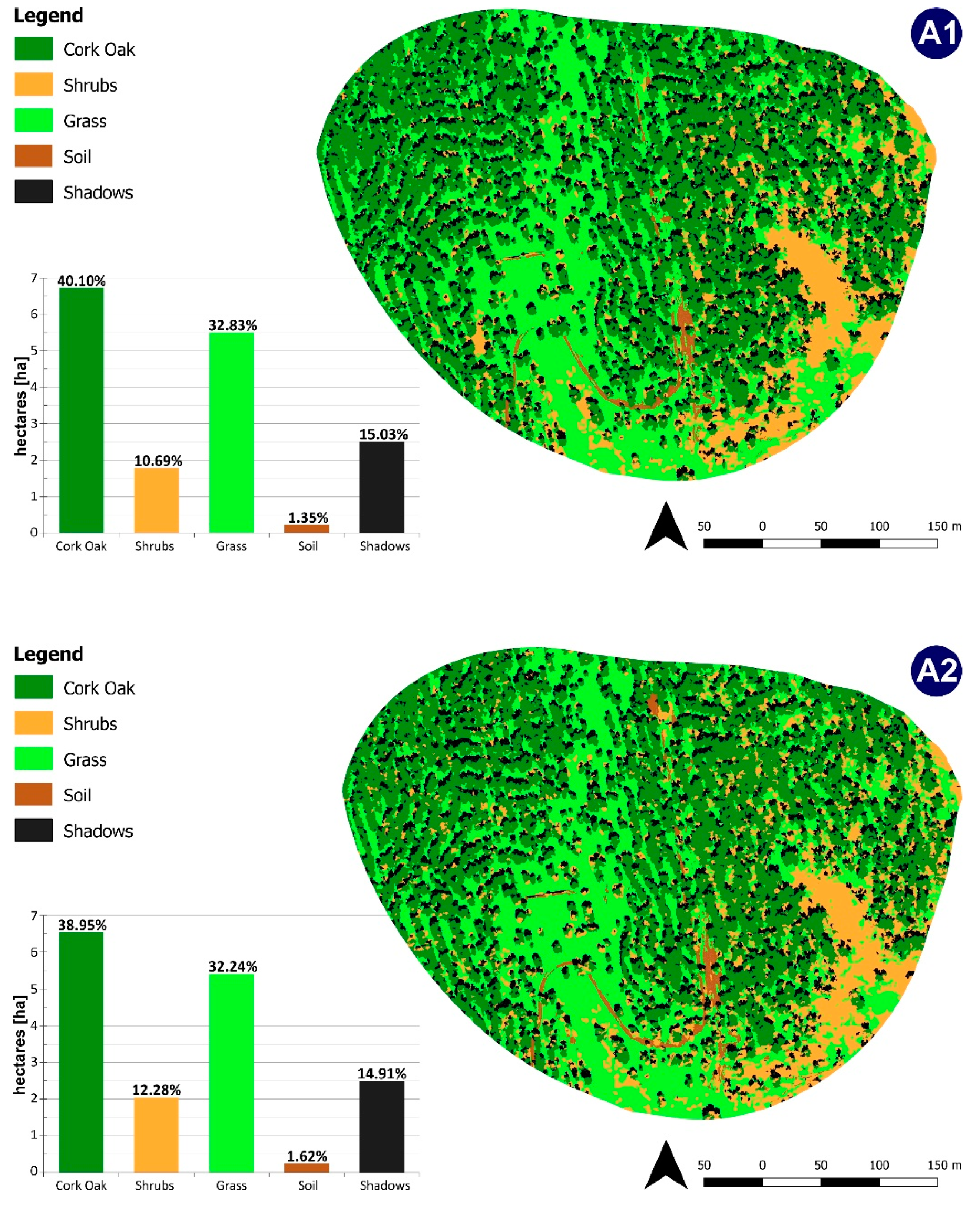
Generally, the quality of the classification can be considered good according to the quality errors, which are intrinsic to the image. This is confirmed by the kappa coefficient, whose values ranged from 0.928 to 0.973 for RF and from 0.847 to 0.935 for SVM. For both spring and summer imagery, the comparison between the SVM and RF algorithms does not reveal large differences in the classification maps, and any differences detected are in very small polygons. However, a comparison of the kappa results with the overall accuracy reveals that the RF algorithm turns out to be more accurate than SVM for both flights, and this is also reflected by the confusion matrix. The most repeated error, particularly in the images classified with SVM, is confusion between the shrubby class and the shadows class, limited to the edges of the shadows. On the contrary, shrubs are clearly distinguished from tree crowns in the whole scene.

The classes, if taken independently, can be analyzed through the user’s and the producer’s accuracy, which indicate commission and omission errors, respectively. For both flights and both algorithms, the cork oak class obtains better classification accuracy, with values that are always higher than 95%. On the other hand, the lowest accuracy is obtained for the shrubs class with the SVM algorithm and the summer flight.

It can be noted from observing the confusion matrix that shrubs are more often confused with shadows or herbaceous vegetation than they are with trees. A preliminary visual analysis is sufficient to notice a common error in all of the maps: some polygons representing the edges of the shadows (at which there is a chromatic transition from the shadow to the adjacent cover) are confused with shrubs, but the confusion of shrubs with grass instead can be justified. It is hard to formulate a reliable assessment of the results for the bare soil class because of the low number of samples, even if the result is representative of the real distribution and width of the class in the whole region (<1.7% of the total surface). The bare soil class is mainly represented by the dirt road present at the site.

Trees and shrubs have similar shapes and spectral features from a nadiral view, and the largest distinction is the height, as well as the epigeal structural form. Thus, the DSM, which has a GSD of 10 cm and underlines the differences in height, plays an important role in discriminating between the two vegetation layers. Moreover, the NDVI is important for the distinction between herbaceous vegetation and shrubs, as well as between the herbaceous layer and bare soil; the NDVI also has a key role in the identification of shrubs. The class separability and thus discrimination provided by these two bands brings additional information, relatively, to the original mosaic bands (R-G-NIR), which is relevant for both processes of segmentation and classification.

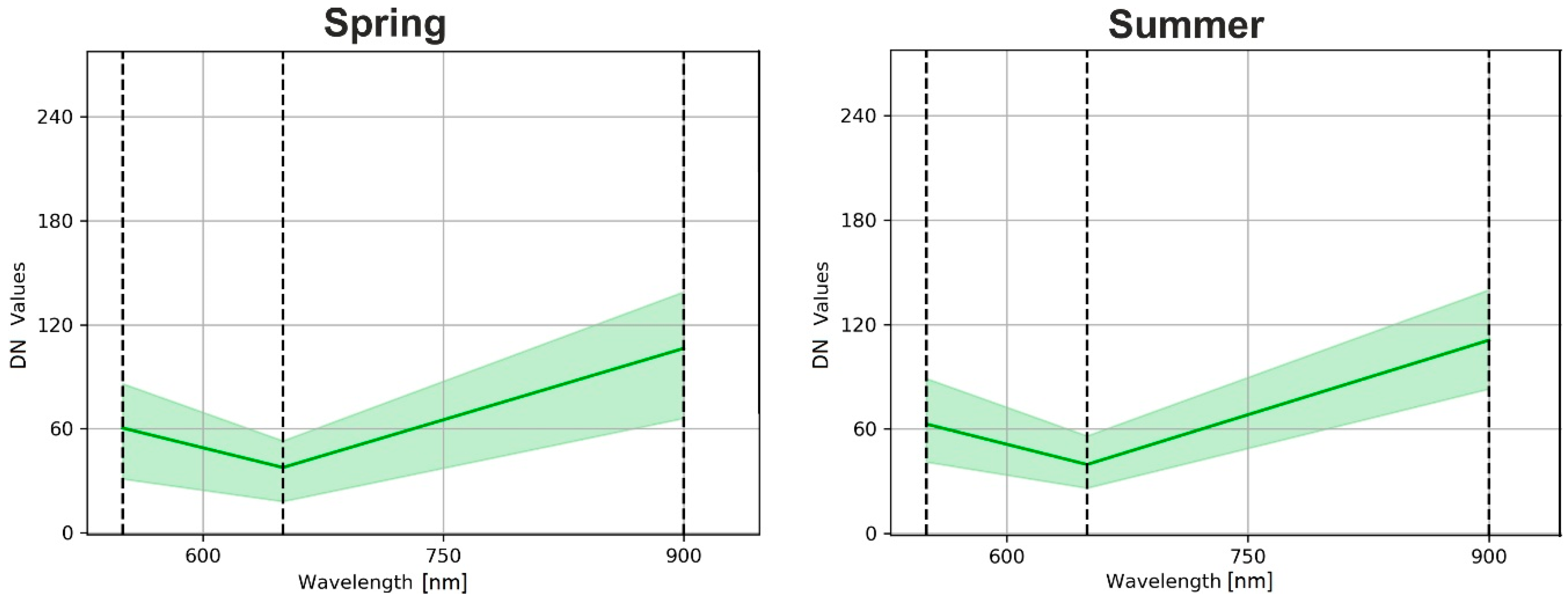
Of the two flight seasons, the spring imagery yielded the best classification in terms of overall accuracy and kappa coefficient according to both classification algorithms. This is mainly because of the features of shrubs, particularly Cistus, which has a tendency to dry out during the summer and can potentially be mistaken for shadows and dry grass. This factor increases the chromatic and the NDVI contrasts among the plants. The opposite happens for herbaceous vegetation, which, during the spring, is in the midst of its photosynthesis activity, while it tends to dry out during the summer; this implies that herbaceous vegetation is classified with lower accuracy in the spring, probably as a result of a lower NDVI contrasting with other photosynthetically active vegetation. Moreover, analysis of the spatial distribution of the classes reveals that the difference between the two classification algorithms for the same season leads to almost the same results, with small differences. Differences between the seasons with the same classification algorithm can be also considered small, and the classifier does not appear to be affected by the cyclical and biological behavior of the species. In fact, with the use of the NDVI information layer, the algorithms similarly distinguished herbaceous vegetation from shrubs, even if they were clearly affected by drought. The larger problem to be faced is related to the large area of shadows in the summer mosaic.

6. Conclusions

Technological development for accurately monitoring vegetation cover plays an important role in studying ecosystem functions, especially in long-term studies. In the present work, we investigated the reliability of coupling the use of multispectral VHR UAV imagery with GEOBIA classification implemented in OTB free and open-source software. Supervised classification was implemented by testing two object-based classification algorithms, random forest (RF) and support vector machine (SVM).

The overall accuracy of the classification was optimal, with overall accuracy values that never fell below 89% and kappa coefficient values that were at least 0.847. Both classifiers obtained good levels of accuracy, although the RF algorithm provided better results than SVM for both images. This process does not seem to have been examined in previous studies; as far as we are aware, this study is the first that uses multispectral R-G-NIR images with DSM and NDVI for the classification of forest vegetation from UAV images using open-source software (OTB).

An open question worth investigating relates to the application of our findings to other forest ecosystems. The OTB suite is free and open-source software that is regularly updated and has proven to provide free processing tools with a steep learning curve coupled with robust results in forest ecosystems that have a complex vertical and horizontal structure. Moreover, as our findings show, OTB can effectively process UAV imagery when implemented on low-power hardware. Therefore, the proposed workflow may be highly valuable in an operational context.

However, some open questions and future research directions remain worthy of investigation. On the one hand, further investigation into the use of smoothing to try to optimize potential usefulness should be carried out in different operational conditions. On the other hand, for the issue with tree shadows, our experience in this study reveals that flight schedules can significantly affect the quality of the obtained imagery, especially in open forest ecosystems such as cork oak woodlands. The summer imagery is affected by about 30% more shadowed area than the spring one.

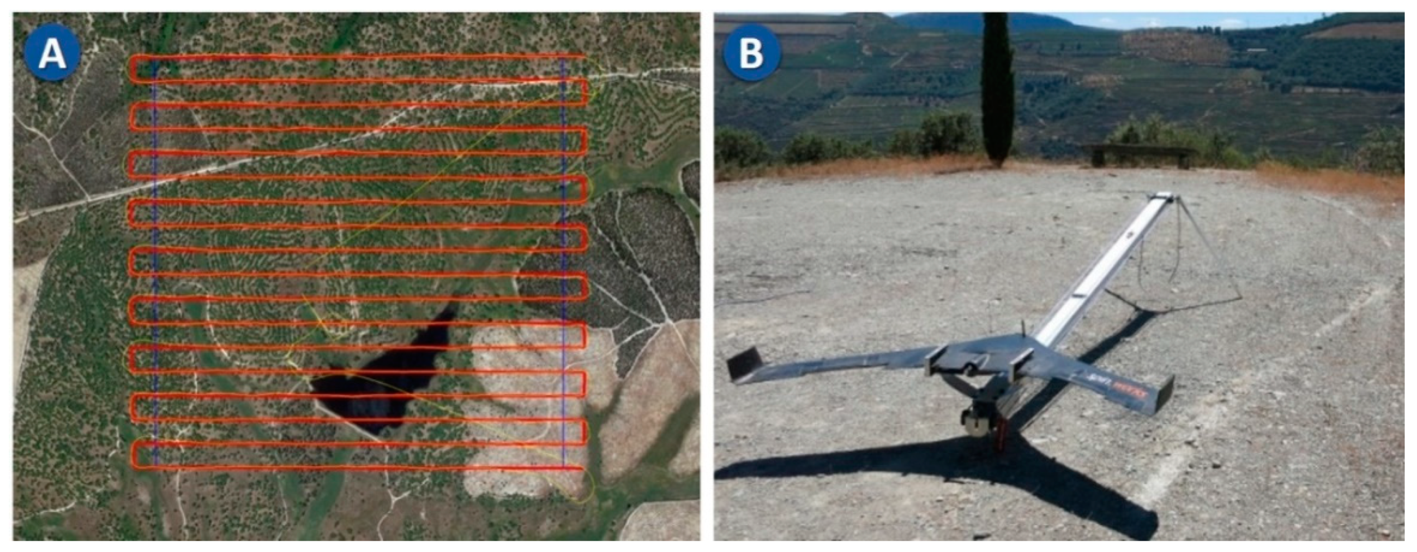
Our findings confirm the reliability of UAV remote sensing applied to forest monitoring and management. Moreover, although a massive amount of UAV hyperspectral and LiDAR data can be obtained with ultra-high spatial and radiometric resolutions, these sensors are still heavy, too expensive, and in most cases require two flights to obtain radiometric and topographic information. Our sensor, which is based on standard R-G-NIR imagery, has the significant advantage of being a very affordable solution in both scientific and operational contexts. Additionally, mounting this sensor on a fixed-wing UAV enables the surveying of surfaces spread over hundreds of hectares in a short time and has thus proven to be a very cost-effective and reliable solution for forest monitoring.

References

1. Modica, G.; Solano, F.; Merlino, A.; di Fazio, S.; Barreca, F.; Laudari, L.; Fichera, C.R. Using Landsat 8 imagery in detecting cork oak (Quercus suber L.) woodlands: A case study in Calabria (Italy). J. Agric. Eng. 2016, 47, 205–215. [Google Scholar] [CrossRef]
2. San-Miguel-Ayanz, J.; de Rigo, D.; Caudullo, G.; Houston Durrant, T.; Mauri, A. (Eds.) European Forest Tree Species; Publication Office of the European Union: Luxembourg, 2016. [Google Scholar]
3. Pádua, L.; Vanko, J.; Hruška, J.; Adão, T.; Sousa, J.J.; Peres, E.; Morais, R. UAS, sensors, and data processing in agroforestry: A review towards practical applications. Int. J. Remote Sens. 2017, 38, 2349–2391. [Google Scholar] [CrossRef]
4. Michez, A.; Piégay, H.; Lisein, J.; Claessens, H.; Lejeune, P. Classification of riparian forest species and health condition using multi-temporal and hyperspatial imagery from unmanned aerial system. Environ. Monit. Assess. 2016, 188, 1–19. [Google Scholar] [CrossRef] [Green Version]
5. Böhler, J.E.; Schaepman, M.E.; Kneubühler, M. Crop classification in a heterogeneous arable landscape using uncalibrated UAV data. Remote Sens. 2018, 10, 1282. [Google Scholar] [CrossRef]
6. De Castro, A.I.; Torres-Sánchez, J.; Peña, J.M.; Jiménez-Brenes, F.M.; Csillik, O.; López-Granados, F. An automatic random forest-OBIA algorithm for early weed mapping between and within crop rows using UAV imagery. Remote Sens. 2018, 10, 285. [Google Scholar] [CrossRef]
7. Yuan, C.; Zhang, Y.; Liu, Z. A survey on technologies for automatic forest fire monitoring, detection, and fighting using unmanned aerial vehicles and remote sensing techniques. Can. J. For. Res. 2015, 45, 783–792. [Google Scholar] [CrossRef]
8. Lehmann, J.R.K.; Nieberding, F.; Prinz, T.; Knoth, C. Analysis of unmanned aerial system-based CIR images in forestry-a new perspective to monitor pest infestation levels. Forests 2015, 6, 594–612. [Google Scholar] [CrossRef]
9. Candiago, S.; Remondino, F.; De Giglio, M.; Dubbini, M.; Gattelli, M. Evaluating multispectral images and vegetation indices for precision farming applications from UAV images. Remote Sens. 2015, 7, 4026–4047. [Google Scholar] [CrossRef]
10. Lisein, J.; Pierrot-Deseilligny, M.; Bonnet, S.; Lejeune, P. A photogrammetric workflow for the creation of a forest canopy height model from small unmanned aerial system imagery. Forests 2013, 4, 922–944. [Google Scholar] [CrossRef]
11. Guerra-Hernández, J.; González-Ferreiro, E.; Sarmento, A.; Silva, J.; Nunes, A.; Correia, A.C.; Fontes, L.; Tomé, M.; Díaz-Varela, R. Using high resolution UAV imagery to estimate tree variables in Pinus pinea plantation in Portugal. For. Syst. 2016, 25. [Google Scholar] [CrossRef]
12. Gini, R.; Passoni, D.; Pinto, L.; Sona, G. Use of unmanned aerial systems for multispectral survey and tree classification: A test in a park area of northern Italy. Eur. J. Remote Sens. 2014, 47, 251–269. [Google Scholar] [CrossRef]
13. Haest, B.; Borre, J.; Vanden Spanhove, T.; Thoonen, G.; Delalieux, S.; Kooistra, L.; Mücher, C.A.; Paelinckx, D.; Scheunders, P.; Kempeneers, P. Habitat mapping and quality assessment of NATURA 2000 heathland using airborne imaging spectroscopy. Remote Sens. 2017, 9, 266. [Google Scholar] [CrossRef]
14. Goodbody, T.R.; Coops, N.C.; Hermosilla, T.; Tompalski, P.; Crawford, P. Assessing the status of forest regeneration using digital aerial photogrammetry and unmanned aerial systems. Int. J. Remote Sens. 2018, 39, 5246–5264. [Google Scholar] [CrossRef]
15. Van Iersel, W.; Straatsma, M.; Middelkoop, H.; Addink, E.; van Iersel, W.; Straatsma, M.; Middelkoop, H.; Addink, E. Multitemporal Classification of River Floodplain Vegetation Using Time Series of UAV Images. Remote Sens. 2018, 10, 1144. [Google Scholar] [CrossRef]
16. Tang, L.; Shao, G. Drone remote sensing for forestry research and practices. J. For. Res. 2015, 26, 791–797. [Google Scholar] [CrossRef]
17. Pádua, L.; Hruška, J.; Bessa, J.; Adão, T.; Martins, L.M.; Gonçalves, J.A.; Peres, E.; Sousa, A.M.R.; Castro, J.P.; Sousa, J.J. Multi-temporal analysis of forestry and coastal environments using UASs. Remote Sens. 2018, 10, 24. [Google Scholar] [CrossRef]
18. Torresan, C.; Berton, A.; Carotenuto, F.; di Gennaro, S.F.; Gioli, B.; Matese, A.; Miglietta, F.; Vagnoli, C.; Zaldei, A.; Wallace, L. Forestry applications of UAVs in Europe: A review. Int. J. Remote Sens. 2016, 38, 1–21. [Google Scholar] [CrossRef]
19. Torres-Sánchez, J.; López-Granados, F.; Peña, J.M. An automatic object-based method for optimal thresholding in UAV images: Application for vegetation detection in herbaceous crops. Comput. Electron. Agric. 2015, 114, 43–52. [Google Scholar] [CrossRef]
20. Teodoro, A.C.; Araujo, R. Comparison of performance of object-based image analysis techniques available in open source software (Spring and Orfeo Toolbox/Monteverdi) considering very high spatial resolution data. J. Appl. Remote Sens. 2016, 10, 016011. [Google Scholar] [CrossRef]
21. Torres-Sánchez, J.; López-Granados, F.; de Castro, A.I.; Peña-Barragán, J.M. Configuration and Specifications of an Unmanned Aerial Vehicle (UAV) for Early Site Specific Weed Management. PLoS ONE 2013, 8, e58210. [Google Scholar] [CrossRef]
22. Goodbody, T.R.H.; Coops, N.C.; Marshall, P.L.; Tompalski, P.; Crawford, P. Unmanned aerial systems for precision forest inventory purposes: A review and case study. For. Chron. 2017, 93, 71–81. [Google Scholar] [CrossRef] [Green Version]
23. Robertson, L.D.; King, D.J. Comparison of pixel-and object-based classification in land cover change mapping. Int. J. Remote Sens. 2011, 32, 1505–1529. [Google Scholar] [CrossRef]
24. Liu, D.; Xia, F. Assessing object-based classification: Advantages and limitations. Remote Sens. Lett. 2010, 1, 187–194. [Google Scholar] [CrossRef]
25. Ma, L.; Li, M.; Ma, X.; Cheng, L.; Du, P.; Liu, Y. A review of supervised object-based land-cover image classification. ISPRS J. Photogramm. Remote Sens. 2017, 130, 277–293. [Google Scholar] [CrossRef]
26. Phiri, D.; Morgenroth, J. Developments in Landsat Land Cover Classification Methods: A Review. Remote Sens. 2017, 9, 967. [Google Scholar] [CrossRef]
27. Blaschke, T.; Hay, G.J.; Kelly, M.; Lang, S.; Hofmann, P.; Addink, E.; Queiroz Feitosa, R.; van der Meer, F.; van der Werff, H.; van Coillie, F.; et al. Geographic Object-Based Image Analysis–Towards a new paradigm. ISPRS J. Photogramm. Remote Sens. 2014, 87, 180–191. [Google Scholar] [CrossRef] [PubMed]
28. Blaschke, T. Object based image analysis for remote sensing. ISPRS J. Photogramm. Remote Sens. 2010, 65, 2–16. [Google Scholar] [CrossRef] [Green Version]
29. Hay, G.J.; Castilla, G. Geographic Object-Based Image Analysis (GEOBIA): A new name for a new discipline. In Object-Based Image Analysis. Spatial Concepts for Knowledge-Driven Remote Sensing Applications; Blaschke, T., Lang, S., Hay, G.J., Eds.; Springer: Berlin/Heidelberg, Germany, 2008; pp. 75–89. [Google Scholar]
30. Hay, G.J.; Blaschke, T. Special issue: Geographic object-based image analysis (GEOBIA). Photogramm. Eng. Remote Sensing 2010, 76, 121–122. [Google Scholar]
31. Franklin, S.E.; Ahmed, O.S. Deciduous tree species classification using object-based analysis and machine learning with unmanned aerial vehicle multispectral data. Int. J. Remote Sens. 2018, 39, 5236–5245. [Google Scholar] [CrossRef]
32. Ahmed, O.S.; Shemrock, A.; Chabot, D.; Dillon, C.; Williams, G.; Wasson, R.; Franklin, S.E. Hierarchical land cover and vegetation classification using multispectral data acquired from an unmanned aerial vehicle. Int. J. Remote Sens. 2017, 38, 2037–2052. [Google Scholar] [CrossRef]
33. CNES OTB Development Team. Software Guide; CNES: Paris, France, 2018; pp. 1–814. [Google Scholar]
34. OTB Development Team. OTB CookBook Documentation; CNES: Paris, France, 2018; p. 305. [Google Scholar]
35. Cerasoli, S.; Costa e Silva, F.; Silva, J.M.N. Temporal dynamics of spectral bioindicators evidence biological and ecological differences among functional types in a cork oak open woodland. Int. J. Biometeorol. 2016, 60, 813–825. [Google Scholar] [CrossRef]
36. Costa-e-Silva, F.; Correia, A.C.; Piayda, A.; Dubbert, M.; Rebmann, C.; Cuntz, M.; Werner, C.; David, J.S.; Pereira, J.S. Effects of an extremely dry winter on net ecosystem carbon exchange and tree phenology at a cork oak woodland. Agric. For. Meteorol. 2015, 204, 48–57. [Google Scholar] [CrossRef] [Green Version]
37. Kljun, N.; Calanca, P.; Rotach, M.W.; Schmid, H.P. A simple two-dimensional parameterisation for Flux Footprint Prediction (FFP). Geosci. Model Dev. 2015, 8, 3695–3713. [Google Scholar] [CrossRef] [Green Version]
38. Soares, P.; Firmino, P.; Tomé, M.; Campagnolo, M.; Oliveira, J.; Oliveira, B.; Araújo, J. A utilização de Veículos Aéreos Não Tripulados no inventário florestal–o caso do montado de sobro. In Proceedings of the VII Conferência Nac. Cartogr. e Geod., Lisbon, Portugal, 29–30 October 2015. [Google Scholar]
39. Cresson, R.; Grizonnet, M.; Michel, J. Orfeo ToolBox Applications. In QGIS and Generic Tools; John Wiley & Sons, Inc.: Hoboken, NJ, USA, 2018; pp. 151–242. [Google Scholar]
40. Grizonnet, M.; Michel, J.; Poughon, V.; Inglada, J.; Savinaud, M.; Cresson, R. Orfeo ToolBox: Open source processing of remote sensing images. Open Geospatial Data Softw. Stand. 2017, 2, 15. [Google Scholar] [CrossRef]
41. Immitzer, M.; Vuolo, F.; Atzberger, C. First experience with Sentinel-2 data for crop and tree species classifications in central Europe. Remote Sens. 2016, 8, 166. [Google Scholar] [CrossRef]
42. Michel, J.; Youssefi, D.; Grizonnet, M. Stable Mean-Shift Algorithm and Its Application to the Segmentation of Arbitrarily Large Remote Sensing Images. IEEE Trans. Geosci. Remote Sens. 2015, 53, 952–964. [Google Scholar] [CrossRef]
43. Li, M.; Ma, L.; Blaschke, T.; Cheng, L.; Tiede, D. A systematic comparison of different object-based classification techniques using high spatial resolution imagery in agricultural environments. Int. J. Appl. Earth Obs. Geoinf. 2016, 49, 87–98. [Google Scholar] [CrossRef]
44. Costa, H.; Foody, G.M.; Boyd, D.S. Supervised methods of image segmentation accuracy assessment in land cover mapping. Remote Sens. Environ. 2018, 205, 338–351. [Google Scholar] [CrossRef] [Green Version]
45. Belgiu, M.; Drǎguţ, L. Comparing supervised and unsupervised multiresolution segmentation approaches for extracting buildings from very high resolution imagery. ISPRS J. Photogramm. Remote Sens. 2014, 96, 67–75. [Google Scholar] [CrossRef] [PubMed] [Green Version]
46. Congalton, R.G.; Green, K. Assessing the Accuracy of Remotely Sensed Data: Principles and Practices; Second CRC Press Taylor & Francis Group: Boca Raton, FL, USA, 2009; Volume 48. [Google Scholar]
47. Cortes, C.; Vapnik, V. Support-Vector Networks Editor. Mach. Learn. 1995, 20, 273–297. [Google Scholar] [CrossRef]
48. Vapnik, V. Statistical Learning Theory; Wiley and sons: New York, NY, USA, 1998. [Google Scholar]
49. Mountrakis, G.; Im, J.; Ogole, C. Support vector machines in remote sensing: A review. ISPRS J. Photogramm. Remote Sens. 2011, 66, 247–259. [Google Scholar] [CrossRef]
50. Adam, E.; Mutanga, O.; Odindi, J.; Abdel-Rahman, E.M. Land-use/cover classification in a heterogeneous coastal landscape using RapidEye imagery: Evaluating the performance of random forest and support vector machines classifiers. Int. J. Remote Sens. 2014, 35, 3440–3458. [Google Scholar] [CrossRef]
51. Hawryło, P.; Bednarz, B.; Wężyk, P.; Szostak, M. Estimating defoliation of Scots pine stands using machine learning methods and vegetation indices of Sentinel-2. Eur. J. Remote Sens. 2018, 51, 194–204. [Google Scholar] [CrossRef] [Green Version]
52. Wessel, M.; Brandmeier, M.; Tiede, D.; Wessel, M.; Brandmeier, M.; Tiede, D. Evaluation of Different Machine Learning Algorithms for Scalable Classification of Tree Types and Tree Species Based on Sentinel-2 Data. Remote Sens. 2018, 10, 1419. [Google Scholar] [CrossRef]
53. Breiman, L. Random forests. Mach. Learn. 2001, 45, 5–32. [Google Scholar] [CrossRef]
54. Cutler, D.R.; Edwards, T.C.; Beard, K.H.; Cutler, A.; Hess, K.T.; Gibson, J.; Lawler, J.J. Random Forests For Classification In Ecology. Ecology 2007, 88, 2783–2792. [Google Scholar] [CrossRef]
55. Trisasongko, B.H.; Panuju, D.R.; Paull, D.J.; Jia, X.; Griffin, A.L. Comparing six pixel-wise classifiers for tropical rural land cover mapping using four forms of fully polarimetric SAR data. Int. J. Remote Sens. 2017, 38, 3274–3293. [Google Scholar] [CrossRef]
56. Kaufman, Y.J.; Remer, L.A. Detection of Forests Using Mid-IR Reflectance: An Application for Aerosol Studies. IEEE Trans. Geosci. Remote Sens. 1994, 32, 672–683. [Google Scholar] [CrossRef]
57. Drăguţ, L.; Csillik, O.; Eisank, C.; Tiede, D. Automated parameterisation for multi-scale image segmentation on multiple layers. ISPRS J. Photogramm. Remote Sens. 2014, 88, 119–127. [Google Scholar] [CrossRef] [PubMed]
58. Clinton, N.; Holt, A.; Scarborough, J.; Yan, L.; Gong, P. Accuracy Assessment Measures for Object-based Image Segmentation Goodness. Photogramm. Eng. Remote Sens. 2010, 76, 289–299. [Google Scholar] [CrossRef]
59. Prošek, J.; Šímová, P. UAV for mapping shrubland vegetation: Does fusion of spectral and vertical information derived from a single sensor increase the classification accuracy? Int. J. Appl. Earth Obs. Geoinf. 2019, 75, 151–162. [Google Scholar] [CrossRef]
60. Díaz-Varela, R.A.; Calvo Iglesias, S.; Cillero Castro, C.; Díaz Varela, E.R. Sub-metric analisis of vegetation structure in bog-heathland mosaics using very high resolution rpas imagery. Ecol. Indic. 2018, 89, 861–873. [Google Scholar] [CrossRef]
61. Marpu, P.R.; Neubert, M.; Herold, H.; Niemeyer, I. Enhanced evaluation of image segmentation results. J. Spat. Sci. 2010, 55, 55–68. [Google Scholar] [CrossRef]
62. Gao, Y.; Mas, J.F.; Kerle, N.; Navarrete Pacheco, J.A. Optimal region growing segmentation and its effect on classification accuracy. Int. J. Remote Sens. 2011, 32, 3747–3763. [Google Scholar] [CrossRef]
63. Yu, Q.; Gong, P.; Clinton, N.; Biging, G.; Kelly, M.; Schirokauer, D. Object-based Detailed Vegetation Classification with Airborne High Spatial Resolution Remote Sensing Imagery. Photogramm. Eng. Remote Sens. 2006, 72, 799–811. [Google Scholar] [CrossRef] [Green Version]
Figure 1. The top figure shows the location of the study area in Central Portugal. Below, the location of the flux tower and the 70% isoline of the footprint climatology representing the study area are identified in a UAV orthomosaic.
Remotesensing 11 01238 g001
Figure 2. Flight plan (red) and flight path (yellow) (A). The fixed-wing UAV S20 before take-off (B).
Remotesensing 11 01238 g002
Figure 3. Workflow of the preprocessing, segmentation, classification, and validation steps implemented to derive an object-based land cover map for cork oak woodlands from UAV imagery.
Remotesensing 11 01238 g003
Figure 4. Visual comparison from some of the numerous tests carried out for the estimation of segmentation accuracy. On the left, a portion of the R-G-NIR image is shown; on the right, the same area is shown with the superimposed vector file containing the segmentation polygons (segments). The top images, from A1 to A3, show the segmentation results obtained without the smoothing step and a range radius of 15 (the default value), 5, and 7. The lower images, B1 and B2, show the segmentation results with the smoothing step and a spatial radius of 5 (the default value) and 30.
Remotesensing 11 01238 g004
Figure 5. Maps of the land cover classification for the spring flight obtained from random forest (RF) (A1) and support vector machine (SVM) (A2) algorithms. Bar charts show the surface distribution according to the five defined land cover classes.
Remotesensing 11 01238 g005
Figure 6. Maps of the land cover classification for the summer flight obtained from random forest (RF) (B1) and support vector machine (SVM) (B2) algorithms. Bar charts show the surface distribution according to the five defined land cover classes.
Remotesensing 11 01238 g006