Coastal Ecosystem Investigations with LiDAR (Light Detection and Ranging) and Bottom Reflectance: Lake Superior Reef Threatened by Migrating Tailings

Abstract

Where light penetration is excellent, the combination of LiDAR (Light Detection And Ranging) and passive bottom reflectance (multispectral, hyperspectral) greatly aids environmental studies. Over a century ago, two stamp mills (Mohawk and Wolverine) released 22.7 million metric tons of copper-rich tailings into Grand Traverse Bay (Lake Superior). The tailings are crushed basalt, with low albedo and spectral signatures different from natural bedrock (Jacobsville Sandstone) and bedrock-derived quartz sands. Multiple Lidar (CHARTS and CZMIL) over-flights between 2008–2016—complemented by ground-truth (Ponar sediment sampling, ROV photography) and passive bottom reflectance studies (3-band NAIP; 13-band Sentinal-2 orbital satellite; 48 and 288-band CASI)—clarified shoreline and underwater details of tailings migrations. Underwater, the tailings are moving onto Buffalo Reef, a major breeding site important for commercial and recreational lake trout and lake whitefish production (32% of the commercial catch in Keweenaw Bay, 22% in southern Lake Superior). If nothing is done, LiDAR-assisted hydrodynamic modeling predicts 60% tailings cover of Buffalo Reef within 10 years. Bottom reflectance studies confirmed stamp sand encroachment into cobble beds in shallow (0-5m) water but had difficulties in deeper waters (>8 m). Two substrate end-members (sand particles) showed extensive mixing but were handled by CASI hyperspectral imaging. Bottom reflectance studies suggested 25-35% tailings cover of Buffalo Reef, comparable to estimates from independent counts of mixed sand particles (ca. 35% cover of Buffalo Reef by >20% stamp sand mixtures).

1. Introduction

An extensive mining legacy is scattered about the northern watersheds and shorelines of the Great Lakes [1,2,3,4]. The Lake Superior Basin is recognized for centuries of iron, copper, zinc, silver and gold mining, historically contributing to the “Industrial Revolution” [5,6,7]. How do the long-term environmental effects of tailings discharges into lakes, rivers and shorelines play out over extended periods of time? Along coastal margins, what is not well known is the progression of impacts as waves and currents move tailings around environments rich in biota. The massive amounts released confound simple arguments of dilution and dissipation. 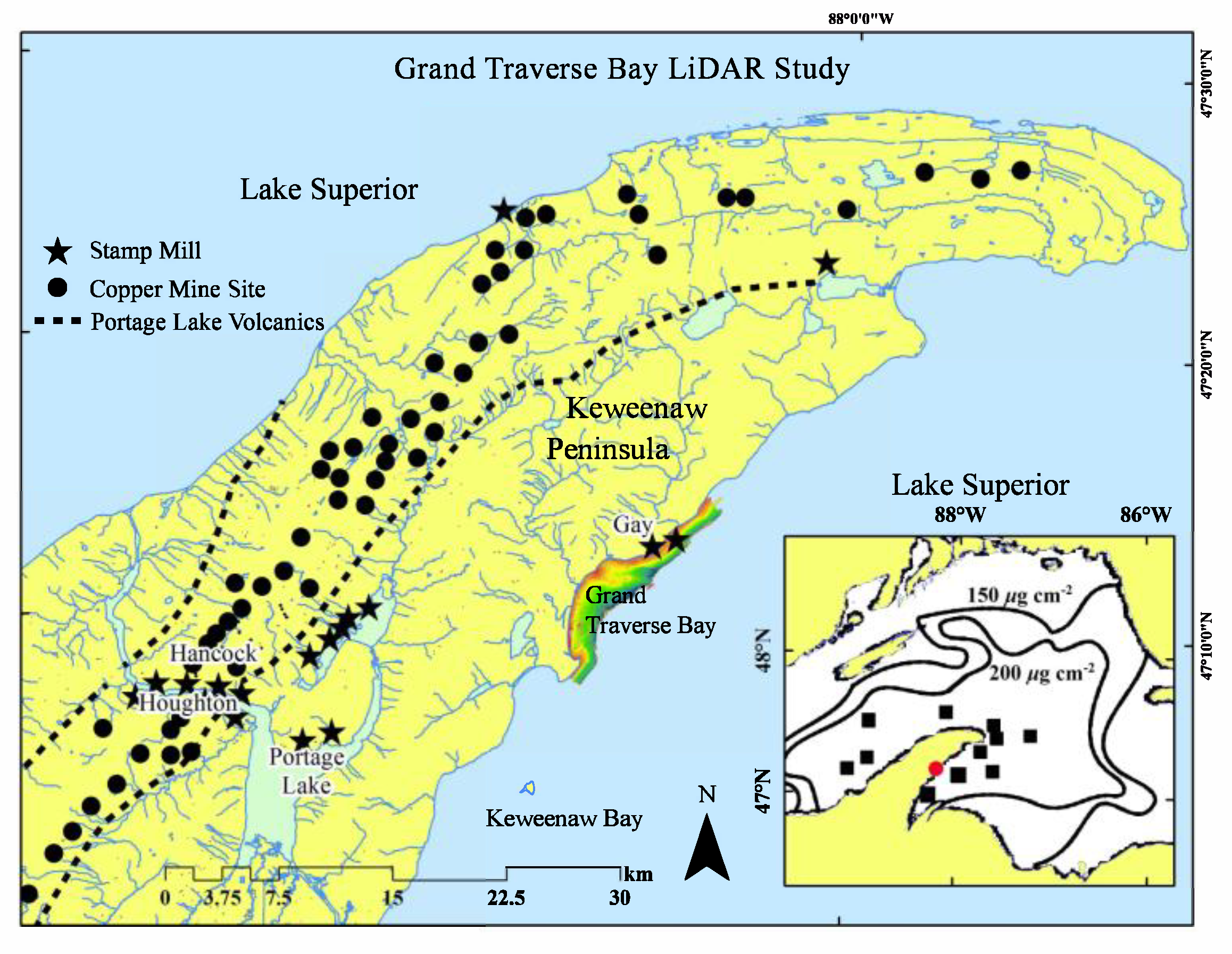Mounting concern about short-term and long-term effects prompted the United Nations Environment Programme report, “International Assessment of Marine and Riverine Disposal of Mine Tailings” [8]. Here we update how LiDAR (light detection and ranging) and bottom reflectance studies help clarify copper tailings movement across a Keweenaw Peninsula coastal site off Lake Superior: Grand (Big) Traverse Bay (Figure 1; green region).

A large metal-rich ‘halo’ exists in sediments around the Keweenaw Peninsula, a consequence of past copper mine discharges [9,10,11]. Stamp mills crushed ore and sluiced tailings (so-called “stamp sands”) into coastal zones. The stamp sands have migrated along extensive stretches of Keweenaw shoreline, impacting critical fish breeding grounds and coastal benthic invertebrate communities, damming stream outlets, intercepting wetlands and recreational beaches [4,12,13,14]. In Grand Traverse Bay (Figure 1), Buffalo Reef is a productive spawning site for lake trout and lake whitefish, contributing an estimated 33% of fish caught in Keweenaw Bay by three tribes (Bad River, Red Cliff and Keweenaw Bay; under the 1842 and 1854 treaties) and recreational fishermen [15]. Moreover, the Keweenaw Bay catch is estimated as 22% of the total southern Lake Superior shoreline commercial catch. The reef is seriously threatened by movement of tailings from the century-old pile off Gay [4,12,16,17].

Figure 1. Geographic location of the Keweenaw Peninsula, Michigan., jutting out into Lake Superior. The position of Grand (Big) Traverse Bay is indicated along the eastern shore of the Keweenaw Peninsula, near Gay, by the red to green contours. On the Peninsula, copper mines are indicated by black dots, stamp mills by stars. Insert shows anthropogenic copper inventory “halo” around the Peninsula, in µg/cm² copper inventory (modified from [12]).

Figure 1. Geographic location of the Keweenaw Peninsula, Michigan., jutting out into Lake Superior. The position of Grand (Big) Traverse Bay is indicated along the eastern shore of the Keweenaw Peninsula, near Gay, by the red to green contours. On the Peninsula, copper mines are indicated by black dots, stamp mills by stars. Insert shows anthropogenic copper inventory “halo” around the Peninsula, in µg/cm² copper inventory (modified from [12]).

Early sonar surveys characterized basic bathymetric features of the Grand Traverse Bay coastal zone. However, the combination of LiDAR and passive bottom reflectance studies provides enhanced visualization of coastal bathymetric features and greatly aids hydrodynamic modeling and ecosystem investigations. Here we update how the two remote sensing techniques complement each other and assess predictions from hydrodynamic modeling. The first technique, LiDAR, is an active remote sensing technique, used over Grand Traverse Bay in the ALS (airborne laser scanning) version, where an airborne laser-ranging system acquires high-resolution elevation and bathymetric data [18]. The Compact Hydrographic Airborne Rapid Total Survey (CHARTS) and the Coastal Zone Mapping and Imaging LiDAR (CZMIL) systems are separate integrated airborne sensor suites used to survey coastal zones, in which bathymetric LiDAR data are collected with aircraft-mounted lasers (Figure 2). In coastal surveys, an aircraft travels over a water stretch at an altitude of 300-400 m and a speed of about 60 m s⁻¹ pulsing two varying laser beams in sweeping fashion toward the Earth through an opening in the plane’s fuselage: an infrared wavelength beam (1064 nm) that is reflected off the water surface and a narrow, blue-green wavelength beam (532 nm) that penetrates the water surface and is reflected off the underwater substrate surface (Figure 2, bottom left). The two-beam system produces a complex wave form (Figure 2, bottom right), that when processed, quantifies the time difference between the two signals (water surface return, bottom return) to derive detailed spatial measurements of bottom bathymetry, in addition to ancillary light scattering data. Laser energy is lost due to refraction, scattering and absorption at the water surface, lake bottom and as the pulse travels through the water column, placing limits on depth penetration. Corrections are incorporated for surface waves and water level fluctuations. Under ideal conditions in coastal waters, blue-green laser penetration allows detection of bottom structures down to approximately three times Secchi (visible light) depth. LiDAR repeatedly achieved around 20–23 m penetration in Grand Traverse Bay, somewhat less than the 40 m recorded from oceanic environments [19,20], yet adequate enough in Lake Superior to clearly characterize the coastal shelf region and highlight critical details of tailings migration.

The second, complementary technique was bottom reflectance scanning (as MSS, multispectral scanning and full hyperspectral). This technique acquires passively reflected light in many discrete spectral bands throughout the ultraviolet, visible, near-infrared, mid-infrared and thermal portion of the spectrum. The technique is important when bottom surfaces reflect enough spectral information to distinguish dominant substrates. Multiple reflectance applications were utilized and compared. Over-flights by the U.S. Department of Agriculture National Agriculture Imagery Program (NAIP) provided 3-band imagery. The CHARTS over-flight package included the Compact Airborne Spectrographic Imager (CASI), a 48-band multispectral to 288-band hyperspectral sensor system. Recently, 13-band multispectral Sentinel-2 orbital satellite data also became available, providing an alternative to NAIP flights. All three sets of data, with appropriate corrections for depth-dependent water column absorption (Lyzenga transformation), were used to map color differences across shallow bottom coastal sediments and to classify substrates. Our studies utilized spectral differences between stamp sands (tailings) and existing natural coastal substrates, in combination with in situ radiance and irradiance studies (Satlantic Optical Profiling Radiometer), to aid the interpretation of bottom classification procedures. The ultimate aim was to independently determine stamp sand cover on Buffalo Reef and to compare with predictions from hydrodynamic modeling.

Ground-truth procedures benefited from numerous photographic ROV surveys and Ponar sediment sample analyses. Ponar sediment samples were examined in the laboratory under a microscope to determine % stamp sand directly from sand mixtures, a classic case of mixed end-members (natural sand, stamp sand). The process created an additional independent check of cover, one that was compared with both hydrodynamic model predictions and bottom sediment classifications. In the process of bottom reflectance investigations, we encountered some problems with deep-water bottom color reflectance (i.e. difficulties during Lyzenga transformations), an aggravation facing many recent deep-water application efforts.

2. Materials and Methods

Canadian Centre for Inland Water (CCIW) Sonar Bathymetry Studies In Grand Traverse Bay. Initial sonar surveys of Buffalo Reef were made by CCIW’s Biberhofer and Prokopec [22], using the RoxAnn sonar survey system. Here we show the results, because they provide independent bathymetric information for cross-comparisons with subsequent LiDAR and bottom reflectance studies. The sounder used for substrate mapping was a digital hydrodynamic Knudsen 320M (Knudsen Engineering Limited), for bottom depths between 2–40 m. The sounder was equipped with a dual frequency (50 kHz and 200 kHz) in-hull transducer, where the 200 kHz frequency was applied towards bathymetry and substrate mapping. Software control of the sounder, data logging and post-survey interrogation were done with proprietary software provided by Knudsen Engineering Ltd. Seabed mapping surveys utilized two RoxAnn units (Sona Vision Ltd, United Kingdom). The units were dedicated to a specific frequency and operated at a set gain for each frequency. Each RoxAnn unit received the return echoes of the Knudsen sounder transmit pulse. To confirm RoxAnn system stability and appropriate signal response, a standard artificial echo was generated with an external pulse generator. The pulse was varied to simulate a range of depths and compared against established values. The signal input was generated using a depth sounder test set (DSTS-4A, Electronic Devices, Inc.). The survey boat ran along a series of NE/SW intersecting transects, with 50 m offsets, for 10 days. During surveys, vessel speed was kept between 2 ms⁻¹ and 5 ms⁻¹, as these speeds were found to be the best operating range for RoxAnn units. A specific NMEA GPS string (NovAtel OEM4 CDGPS) was logged to record the accuracy of the vessel’s location. Expected 2D positional accuracy was 1–2 m. Positional data and input from the RoxAnn units were integrated using either the marine software package Microplot (Sea Information Systems, United Kingdom) or Hypack (Hypack Inc., CT, USA). For ground-truth, a combination of underwater video (auto-iris underwater camera, Ocean Systems Ltd., WA, USA) and sediment sampling (Shipek) was used to check acoustic classes of sediment. For more detailed discussion of procedures and results, see References [16,22].

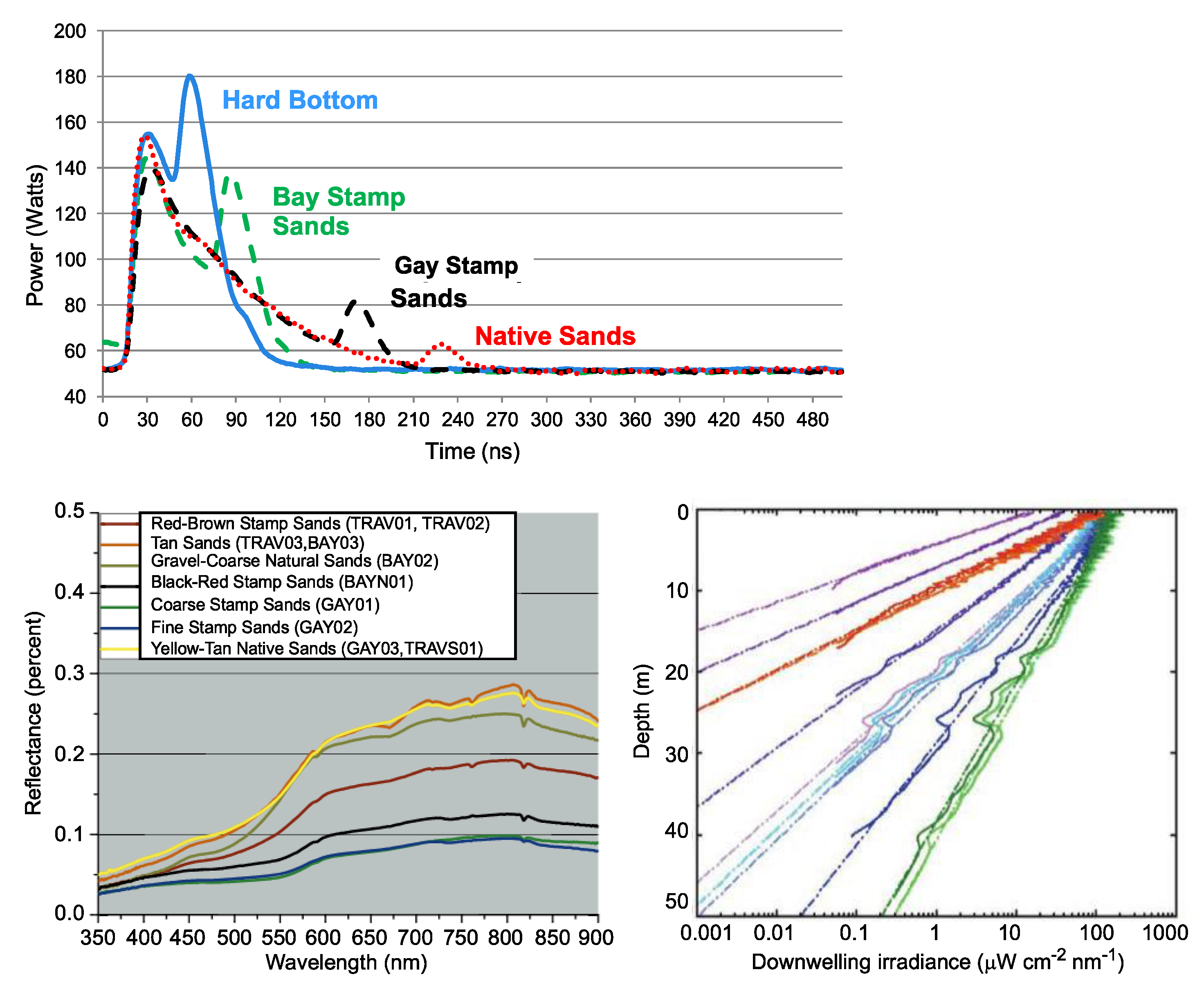
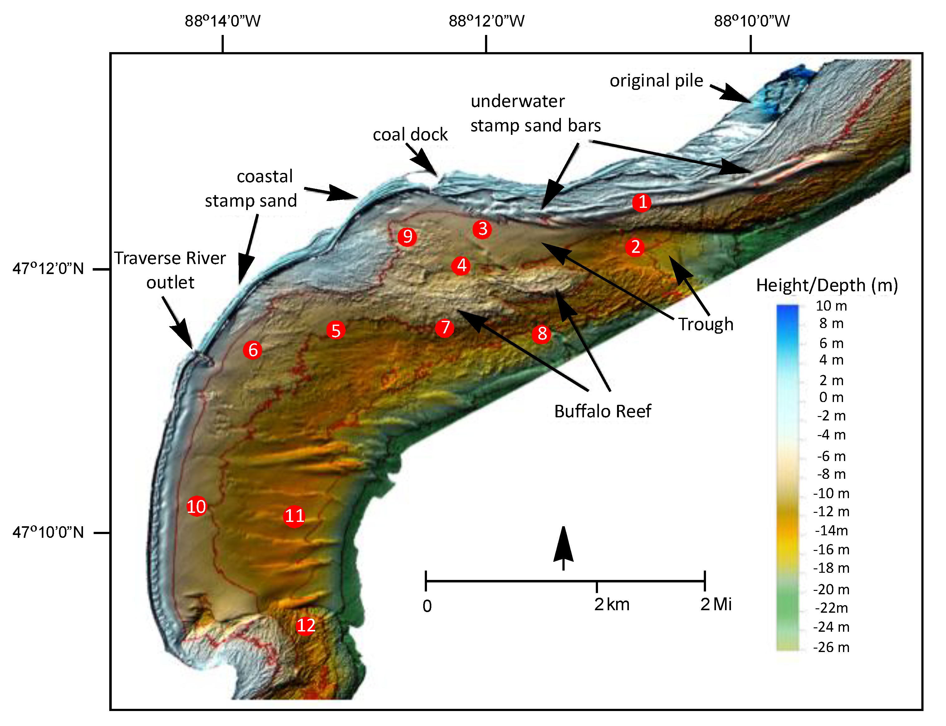
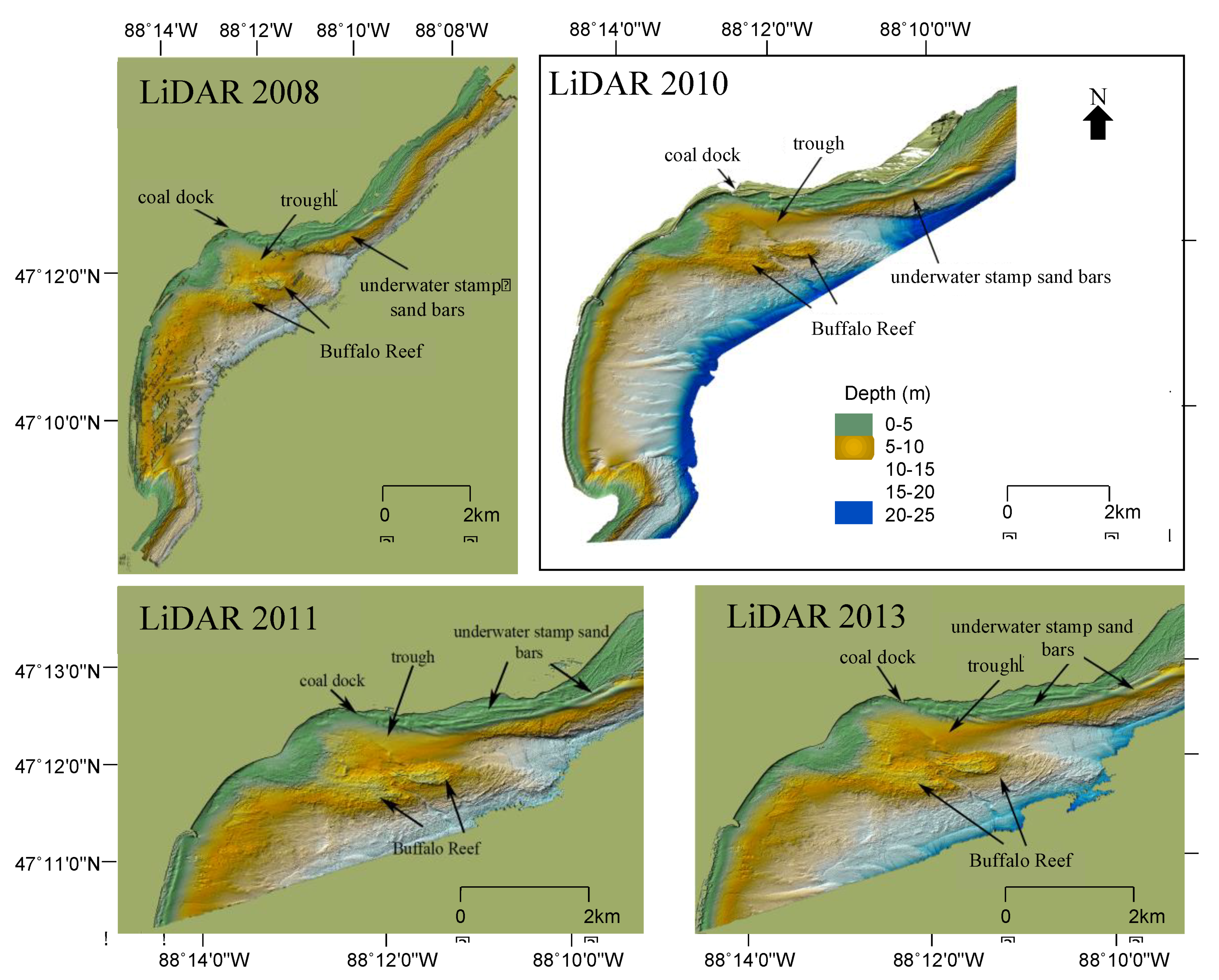
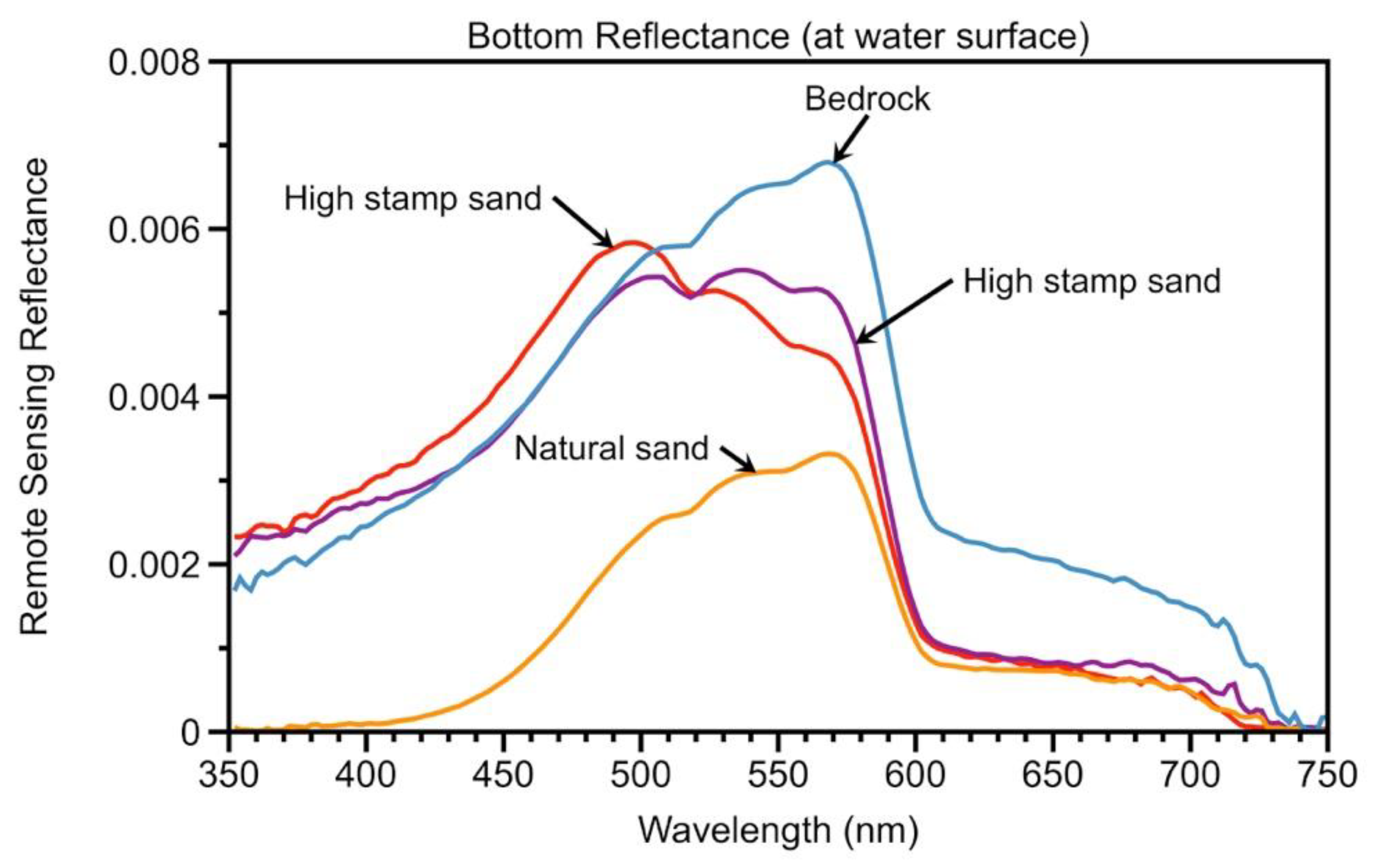
LiDAR Digital Elevation Models (DEMs). Data from aerial photographs (1938–present) and five LiDAR over-flights (2008, 2010, 2011, 2013, 2016) addressed migration of tailings along the shoreline and across Grand Traverse Bay. Quantification included above-water movement along beach margins (aerial photography, NAIP, LiDAR) as well as underwater movement across the coastal shelf and onto Buffalo Reef (LiDAR and bottom reflectance studies). Initial plots of wave-form suggested decent recovery from all three major bottom types: stamp sand, natural sand and bedrock (Figure 3, top). The LiDAR studies provided vital information about specific bathymetric features, including migration of large underwater stamp sand bars. Four of the airborne surveys (2008, 2011, 2013, 2016) were conducted by the U.S. Army Corps of Engineers Joint Airborne LiDAR Bathymetry Technical Center of Expertise (JALBTCX), using the CHARTS (2008 and 2011) and CZMIL (2013 and 2016) sensor suites. Concurrent ground truth measurements (Ponar sediment sampling; ROV transects; spectral substrate characterization, Figure 3, bottom left) provided validation of substrates, detection of stamp sands and especially quantification of stamp sand percentages in sand mixtures and Cu concentrations. The detailed LiDAR bathymetric sampling from 2008 to 2016 allowed DEM (Digital Elevation Map) construction, documenting stamp sand encroachment onto Buffalo Reef. The second airborne survey (2010) came from the National Oceanic and Atmospheric Administration (NOAA) through the Great Lakes Restoration Initiative (GLRI) authorized bathymetric LiDAR data collection. The data were collected and made available by the Fugro LADS Mk II system in CHARTS format by the Fugro LADS Mk II system. Combining and comparing LiDAR and additional MSS bottom reflectance data allowed updated, comprehensive estimates of bathymetry, assistance in hydrodynamic modeling of particle deposition and clarification of regions covered by migrating stamp sands.

The JALBTCX sensor suites used for airborne coastal mapping and charting in the Great Lakes include CHARTS and CZMIL [23]. CHARTS features a 3-kHz bathymetric LiDAR, whereas CZMIL includes a 10-kHz bathymetric LiDAR (green laser in the 532 nanometer wavelength). The systems measure water depths up to two to three times Secchi depth in which CHARTS is capable of 5-m spot spacing, ±30-cm vertical accuracy and CZMIL is capable of 0.7-m spot spacing in shallow water, 2-m spacing in deep water and ±15-cm vertical accuracy [24,25]. Both CHARTS and CZMIL include an integrated Itres (CASI)-1500 for passive hyperspectral imaging in which many narrow, contiguous spectral bands are scanned across the electromagnetic spectrum [26]. CHARTS is a NAVOCEANO-owned asset shared with the US Army Corps of Engineers [27]. LiDAR DEMs and CASI hyperspectral image products (further described in [23]) for 2008, 2011, 2013 and 2016 were provided by JALBTCX for analysis. Statistical analysis of wave forms (Figure 2, bottom right) checked for substrate-specific features. The GIS-referenced high-resolution LiDAR DEM portion of the data set was used to construct 2 m² resolution LiDAR bathymetry maps for the region around Buffalo Reef (2008–2013). We used remote sensing processing software, ENVI 4.7, for all image-processing procedures. The strips were mosaicked and re-projected. For distance, aerial and volume calculations, the data was re-projected to the appropriate local, Universal Transverse Mercator (UTM, projection = WGS84, zone = 16) coordinate system.

For the 2016 DEMs at MTRI, rasterized topobathy LiDAR elevations were obtained from CZMIL in the International Great Lakes Datum of 1985 (IGLD-85). The individual files were mosaicked together in ArcMap using the Mosaic to New Raster tool. The mosaicked image was re-projected into NAD1983_UTM_Zone_16N with the Project Raster (Data Management) tool and the resampling technique was set to bilinear. The Raster Calculator was used to adjust the elevation data to height and depth by subtracting the average mean water level, 183.735 m, on September 20, 2016, obtained from the NOAA tide gauge in Marquette, MI (https://tidesand currents.noaa.gov/).

In addition to aerial photographic reconstruction of early erosion and deposition trends (up to 2008, see References [12,14,17]), mosaicked LiDAR data from multiple over-flights (2008–2016) also allowed detailed estimates of shoreline erosion and deposition. Difference calculations of underwater stamp sand bar volume, mass and movement could be measured, quantifying details of stamp sand bar erosion and deposition (e.g., [17,28]). LiDAR DEM surfaces also provided excellent bathymetric maps for hydrodynamic modeling [29]. Bottom reflectance studies of stamp sand cover could be compared with hydrodynamic model predictions. Here we discuss the nature of hydrodynamic modeling in the bay and attempt to determine modern-day quantitative stamp sand cover of Buffalo Reef. For a cross-check on the accuracy of bathymetric measurements, LiDAR-derived depths were cross-compared with the georegistered National Water Resources Institute (NWRI) SONAR-derived depths and sediment classification maps (Biberhofer and Procopec 2008). We used statistical software packages (SYSTAT, OriginPro) for determining initial spatial cross-correlations. For example, when 2008 LiDAR-derived bathymetry was compared to NWRI bathymetry, correlations were: R² = 0.98).

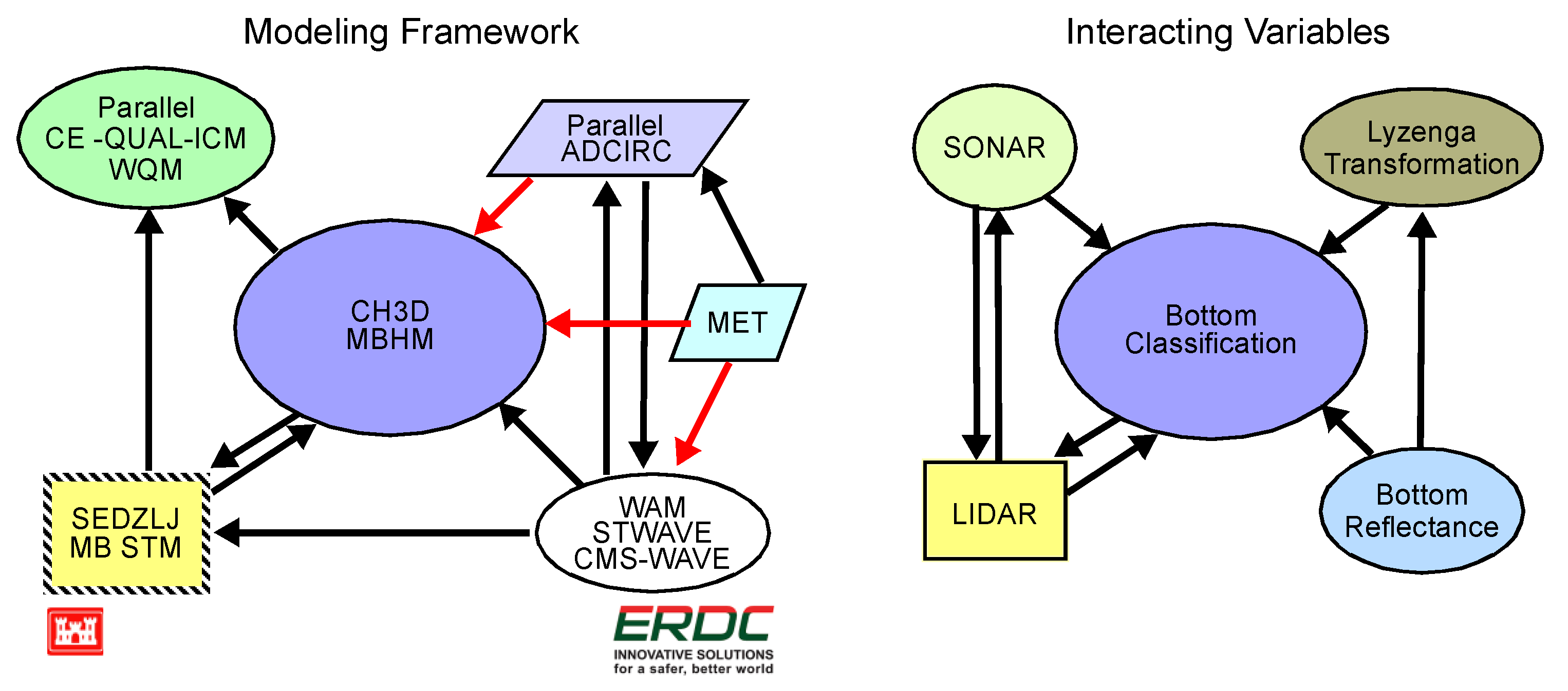
USACE ERDC-EL/ERDC-CHL (Vicksburg) Hydrodynamic Model of Sediment Transport 1n Grand Traverse Bay. The U.S. Army Engineer Research And Development Center Corps (ERDC-EL) utilized the Geophysical Scale Transport Modeling System (GSMB) to model hydrodynamic features and sediment transport in Grand Traverse Bay. The model framework of GSMB is shown in Figure 4, indicating that ERDC-EL accepted wave, hydrodynamic, sediment and water quality transport sub-models that were both directly and indirectly linked. The components of GSMB were: (1) the 2D deep water wave model WAM [30,31], shallow water wave models STWAVE [32] and CMS-WAVE [33], (2) the large-scale unstructured 2D ADCIRC hydrodynamic model (http://www.adcirc.org) and the regional scale models CH3D-MB [34], which is the multi-block (MB) version of CH3D-WES [35,36], 3) MB CH3D-SEDZLJ sediment transport model [37] and 4) CE-QUAL-ICM water quality model [38,39]. For this study, a subset of GSMB components was applied, where the meteorologically forced WAM provides the deep water wave forcing to CMS-WAVE, which in turn provides radiation stress gradients, wave heights, periods and directions forcing to MB CH3D-SEDZLJ. In addition, open water surface elevation forcing is provided to CH3D-SEDZLJ by the lake-wide ADCIRC simulations. Details of equations and calibrating simulations are provided in Hayter et al. [29].

Meteorological forcing utilized archived data. The NCEP Climate Forecast System Reanalysis (CFSR) archive is based on a re-analysis program of all meteorological products generated by NOAA’s National Center for Environmental Predictions (http://rda.ucar.edu/pub/cfsr.html). This 33-year archive (1979–2011) provides wind and pressure on a Gaussian grid with a resolution of ca. 38 km and barometric pressure fields on a 0.5 deg global geographical resolution at one-hour intervals. The Lake Superior wind and pressure fields were downloaded, interpolated from the Gaussian grid to a spherical grid with a resolution of 0.02 deg in both longitude and latitude and reformatted by Oceanweather Inc. under contract to LRE for a 2012 FEMA project. The existing ADCIRC storm surge model bathymetry and grid, provided by the FEMA Modeling Contractor STARR (2012), was applied to Grand (Big) Traverse Bay. Additional grid improvement and refinement was implemented throughout Grand (Big) Traverse Bay and the Gay tailings pile site. Extensive initial calibration and validation included storm event simulations (November 1994, November 1998, April 2004, April 2008, 1 March–30 November 2012; [29]).

Previous single-block applications of combined hydrodynamic and sediment transport models required long computer processing time as well as large memory storage requirements. This is because in structured grids with complicated geometries, the number of active cells (water) is often much smaller than the number of inactive cells (land). Both of these issues were overcome by implementation of single-block grid decomposition and Message Passing Interface (MPI) subroutines, which provide the multi-block (MB) grid capability [40]. The MB grid approach runs each grid in parallel computations, where each grid block is assigned to a separate CPU or processor. Message passing allows the exchange of computational field information, such as the water level elevation, velocity component and constituent arrays, between adjacent grid blocks. The advantages of the MB grid parallel approach include: (1) the flexibility of site-specific horizontal and vertical grid resolution assigned to each grid block, (2) block-specific application of the sediment transport, wave radiation stress gradient forcing and computational cell wetting/drying model options and (3) reduced memory and computational time requirements allowing larger computational domains and longer simulation time periods.

The MB grid developed for the stamp sand project covered the region of Lake Superior from the northeast tip of the Keweenaw Peninsula to the coastline near Big Bay Point Lighthouse. The design of the grid system allowed (1) a boundary forcing sufficiently remote to the stamp sands Gay site, (2) increasing grid resolution as one approaches Grand Traverse Bay and (3) high resolution in the project area (10–20m). The initial bathymetry utilized in grid development was based on 2008 LiDAR survey data [12], in which the trough to the north and northwest of Buffalo Reef was characterized in detail. Additional CMS-Wave model domains and depth contours were based on 2010, 2011, 2013 LiDAR data [14,17]. Wind data for the south central Lake region were available from six NOAA stations: Grand Traverse Bay (GTRM4), Big Bay (BIGM4), Marquette (MCGM4), Stannard Rock (STDM4), Buoy 45004 and Buoy 45025. Buoy 45025 is relatively new (deployed June 2011) compared to the other five stations (prior to 2008). Great Lakes buoys are typically deployed from late spring to late fall, to avoid ice conditions. Wave data were available from Buoys 45004 and 45025 (directional). Additional wave information for Lake Superior was available from two databases; (1) 34 years hind-cast database (1979–2012) from the Wave Information Study (WIS) and (2) about 8 years (2006–2114) now-cast data from the Great Lakes Coastal Forecasting System (GLCFS; http://www.glerl.noaa.gov/res/glcfs/). Data from Seven WIS Stations were available off the Grand (Big) Traverse Bay coastline site. Data from GLCFS and WIS are cross-compared in Hayter et al. [29], including wind and wave rose diagrams for the 34-year hindcast data. Extreme waves approaching the Stamp Sand Beach at Gay come more from the East direction with a maximum 34-year wave height equal to 4.7 m and wave period of 9.7 sec (25-year return period). A total of 28 wave simulations were conducted, including 14 non-storm simulations and 14 storm simulations. For the non-storm cases, two time periods of May-August (4 months) and October-November (2 months) were modeled in 3-hr intervals for 2008, 2010, 2011 and 2013. For the storm cases, seven historical storms, with durations from 10 days to 3 weeks, between 1985 and 2007, were selected and modeled at 1-hr intervals.

The sediment transport model in GSMB is the SEDZLJ sediment transport model [41,42]. SEDZLJ is an advanced sediment bed model that represents the dynamic processes of erosion, bed-load transport, bed sorting, armoring, consolidation of fine-grain sediment dominated sediment beds, settling of flocculated cohesive sediment, settling of individual non-cohesive sediment particles and deposition. SEDZLJ is dynamically linked to CH3D-MB in that the hydrodynamics and sediment transport modules are run during each model time step. A full description of SEDZLJ is provided in Hayter et al. [29]. The SEDZLJ sediment model was set up to simulate sediment transport and deposition in the GSMB model domain, using available sediment data (

Table 1. Example of native and stamp sand size classes and percentages. Both site-specific size distributions and percentages of native sand and stamp sand (Ponar samples) were used in calculations. Specific gravities (Native sand = 2.65; Stamp sand = 2.9).

Sediment Type	Percent Sediment Size Class (Size, µm)							Total
	Silts	100	188	375	750	1500	3000
Native Sediment	3	17	40	20	10	-	10	100%
Stamp Sands	2	-	3	12	58	20	5	100%

; example of grain size distributions and specific gravities) for stamp sand deposits, Buffalo Reef and the shoreline and surf zone along the shoreline between the Gay tailings pile and Traverse River harbor. For the current modeling study six size classes were used to represent the size distribution of stamp sands (20, 188, 375, 750, 1500 and 3000 µm) and native sands (20, 100, 188, 375, 750 and 3,000 µm). Based on analysis of sediment grab samples and shoreline samples, the specific gravities of stamp sands and native sands were 2.90 and 2.65, respectively. The settling velocities for the seven different sediment size classes were determined. Erosion loss from the face of the initial Gay pile came from previous calculations and predictions, based on aerial photographs and LiDAR determinations [12,14,17]; plus 2016 over-flight). The deposition rate for a particular size class was determined by multiplying the settling velocity by the suspended sediment concentration of that size class in the bottom layer. The probabilities of deposition for all size classes were set equal to one [43].

Sand Particle End-members And Mixtures. The crushed Portage Lake Volcanics are basalts (K,Fe,Mg plagioclase silicates; augite and minor olivine), whereas the Jacobsville Sandstone is composed chiefly of quartz particles, that is, very different end-members. The erosion rates of the 12 sediment size classes in the SEDZLJ followed Roberts et al. [44], who measured erosion rates of quartz particles in a SEDFLUME. SEDFLUME is a field- or laboratory-deployable flume for measuring erosion rates of cohesive and non-cohesive sediment beds (McNeil et al. 1996). The erosion rates for the five stamp sand size classes were adjusted by dividing the erosion rates, following Roberts et al. 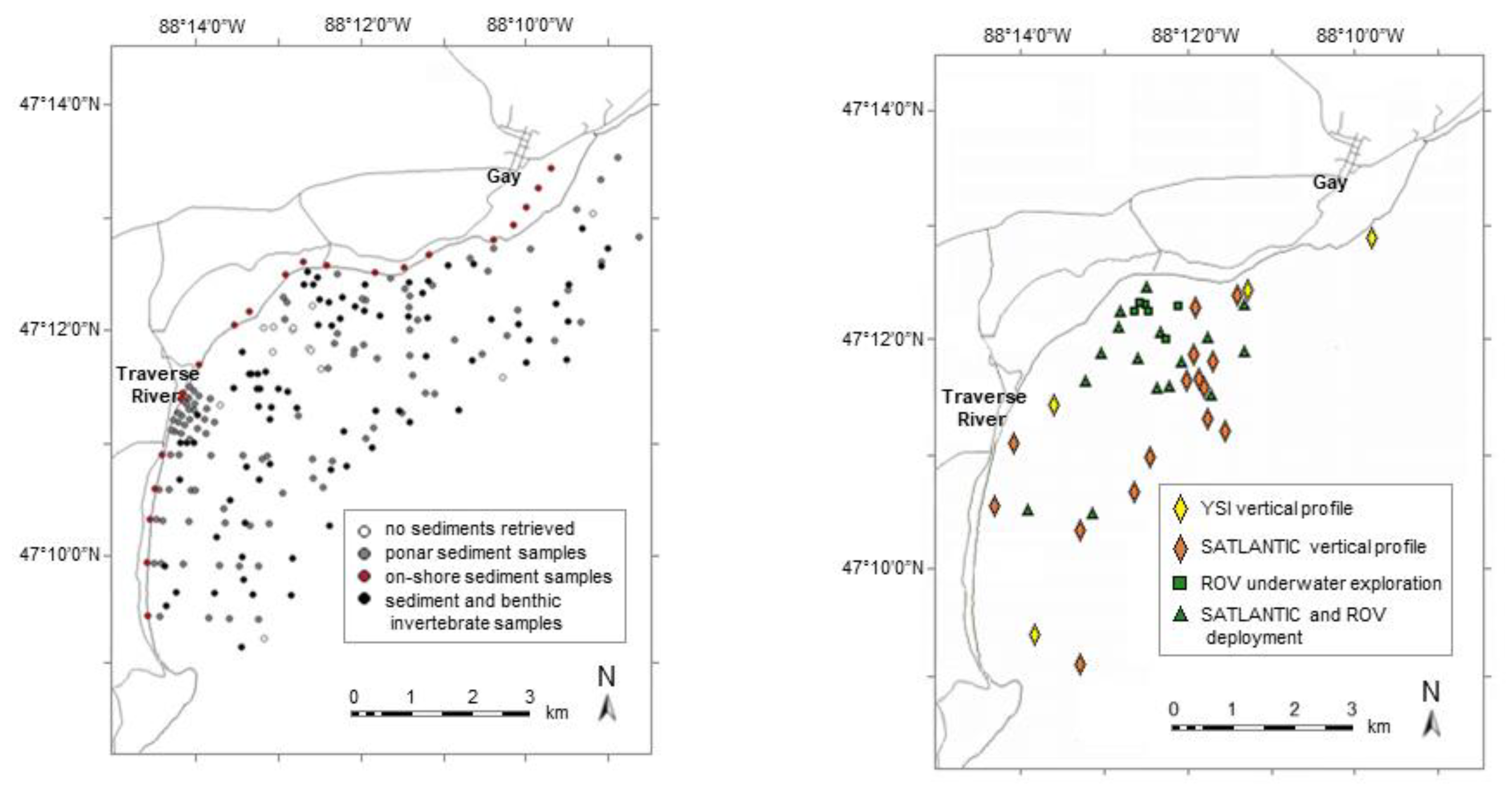[44], by the ratio 2.9/2.65, that is ratio of specific gravities. The spatially varying composition of the sediment bed in grid blocks came from all available sediment data, including the detailed 2013 Ponar survey (Figure 5, left). No sediment data were available for certain blocks, either because sampling showed non-erodible sediment (e.g., outcropping Jacobsville Sandstone bedrock or coarse erratic gravels/boulders) or sites were far removed from Grand (Big) Traverse Bay (deep-water clay-sized bottom sediments), both unlikely to contribute to short-term sediment fluxes.

As an important, independent check, we conducted a grain classification and count approach on Ponar mixed sand samples. Because the two principle sand types in the bay come from quite different sources, under a microscope (Olympus LMS225R, 40-80X), particle grains from the 2013, 2016 and 2017 Ponar samplings could be separated into crushed opaque (dark) basalt versus rounded, transparent quartz grain components, allowing calculation of % stamp sand particles in particle (sand) mixtures. Percentage stamp sand values were based on means of randomly selected subsamples, with 3–4 replicate counts, 300 total grains in each count.

NAIP, Sentinel-2 and CASI Multispectral-Hyperspectral Reflectance Studies. Although there were scattered Ponar grab-samples and ROV photo-transects for ground-truth, initial studies utilized underwater bottom reflectance as a way to determine substrate classification and stamp sand cover. Stamp sands (crushed Portage Lake Volcanics basalt) on the beach have a relatively low albedo compared to natural white beach sands (naturally derived from Jacobsville Sandstone) and both have distinctive spectral characteristics. In original investigations, rather than utilize the 2008 CHARTS over-flight data, which included CASI hyperspectral, there were complicating annoyances from sun-glint artifacts. Therefore, we chose a 3-band 2009 NAIP over-flight for the initial shallow-water substrate classification. Default NAIP features red (604–664nm), green (533–587nm) and blue (420–492nm) bands. Since 2007, there is also near-infrared (833–887nm). The 3-band spectral reflectance allowed construction of three primary underwater substrate types along the coastal margins: stamp sands, natural beach sands and Jacobsville Sandstone bedrock [12,14,17]. Surface spectral signature procedures followed those described by Sabol et al. [45], using an Analytical Spectral Device (ASD), Inc., FieldSpec Pro (model FSP350-2500PJ). Spectral signatures for the three substrate types in shallow water are shown in Figure 3 (bottom left). Here we review the original substrate classification, which appeared in Kerfoot et al. [12,14] and superimpose Buffalo Reef outlines to estimate percentage stamp sand cover.

To quantify down-welling and upwelling spectral irradiance in shallow and deeper waters, several variables are critical parameters. Water reflectance of the optically deep water (ρ_∞) and the shallow water (ρ_w) and bottom reflectance (ρ_b) are defined respectively as:

ρ_w = πL_w/E_d0, ρ_∞ = πL_∞/E_d0, ρ_b = πL_b/E_dz

(1)

where L_w is the water-leaving radiance in the presence of the bottom, L_∞ is the water-leaving radiance for an infinitely deep water column, L_b is the radiance reflected by the bottom and E_do and E_dz are the downwelling irradiance at the surface and bottom, respectively.

Checks on general bottom reflectance were quantified using a Satlantic OC P1000 Optical Profiling Radiometer (for an example of field down-welling spectra, see Figure 3, bottom right). The Satlantic work provided attenuation coefficients for down-welling and upwelling spectral bands. Critical additional variables were surface irradiance energy and coefficients for depth-dependent spectral transmission. Once solar irradiance penetrates the water surface, it decreases exponentially with depth (z) according to the Beer-Lambert Law, and is a function of wavelength (λ), E_dz = E_do(z=0-)e^−Kdz where E_dz and E_d0(z=0-) are the downwelling irradiance at depth z and just below the water surface, respectively. K_d (m⁻¹) is the diffuse attenuation coefficient of the downward irradiance defined in terms of the decrease of the ambient downwelling irradiance (E_d) with a depth that comprises photons heading in all downward directions; K_d(λ) varies vertically with depth. However, for resolution of bottom reflectance, ambient light must reflect off the bottom surface and return a signal to the surface plane, hence the importance of the Satlantic upwelling irradiance measurements. ArcMap software package (originally version 9.3, now 10.2.1) was used to create a depth-dependent mask that was superimposed upon the reflectance data to check the ability of various sensors to resolve substrate color contrasts. Lyzenga’s [46] method was used for depth-correcting radiance [12,47].

Lyzenga [46] provided an early procedure for handling reflectance depth effects in multi-band imagery, allowing the construction of a water depth-independent mosaic (GIS substrate classification). The method assumes that bottom reflectance in band i (L_b,i) is an exponential function of depth and attenuation coefficient in the band (K_d,i). Given that depth in a pixel is constant for all bands, the algorithm attempts to linearize the relationship between radiance in two bands i and j and water depth. The main assumptions are that: (1) differences in radiances between different pixels for the same substrate are due to differences in depth; and (2) K_d is constant for each band. The first step is to select pixel samples for the same bottom at different depths and plot (ln(L_TOA,i − L_TOA,_∞,i)) versus (ln L_TOA,j − L_TOA,∞,j). The slope of the regression corresponds to a proxy of the attenuation coefficient ratio K_d,i/K_d,j that is a constant value for any substrate. Preliminary plots suggested good ratio-dependence with relatively shallow depths. Ratio-based algorithms determine the relation between different spectral bands over the same bottom type with varying depth. The polygons are then classified by substrate type. By applying this method, we were able to separate different bottom types based on their reflectance. The MSS images were projected to UTM zone 16 coordinate system and pixel values converted to actual spectral reflectance values (watts/m²) for comparison with Satlantic data. ArcGIS and ERDAS IMAGIN image processing software were then used to translate data from images (three data sets: 2009 3-band National Agricultural Imagery (NAIP) over-flight; 2016 13-band Sentinel-2 ocean color satellite data; 2008 and 2016 48-band CASI over-flight). Passive color substrate classifications identified spatial regions covered by stamp sands.

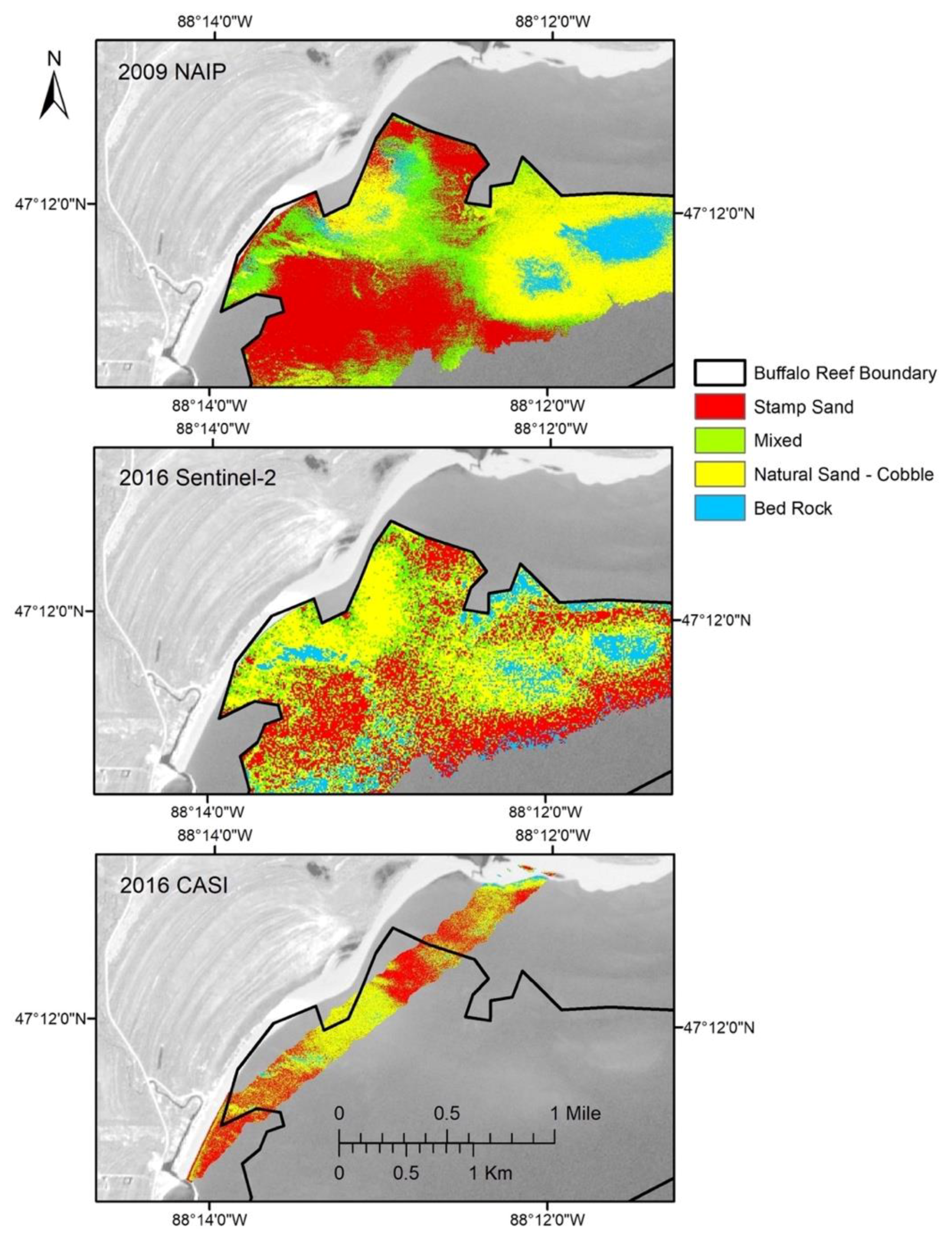
One of the major objectives was to assess the utility of airborne multispectral and hyperspectral imagery to map stamp sand extent and percentage cover on Buffalo Reef. One difficulty with the prior 2009 NAIP sediment classification mapping scheme was that it used a limited number (3) of high bandwidth spectral channels. We hoped to use NAIP imagery again for cross-comparisons, only to find that two later NAIP over-flights had serious problems with heavy seas and resuspended material. For this reason, we utilized 2016 13-band Sentinel-2 satellite data for constructing bottom type maps to compare with the 2009 NAIP map. Sentinel-2 data were satellite procured with less spatial resolution than the original NAIP or LiDAR data, producing differently pixelated surfaces. Another issue in all three spectral reflectance techniques was that they were much more seriously constrained by depth penetration than LiDAR DEMs. Because passive light penetrates much less deeply than LiDAR, the area of the reef covered was reduced. Moreover, the ability of deep-water columns to differentially absorb and scatter longer wavelengths (λ) greatly hindered accurate substrate classification.

Another major issue in the study was that underwater sand deposits vary in stamp sand percentages across the bay, mixing original substrate end-member classification categories. However, the Compact Airborne Spectrographic Imager (CASI) provided potentially both high spatial and spectral resolutions. We explored whether 2016 CASI full 288-channel hyperspectral imagery could help deal with different mixtures of stamp and native sands. The spectral range covered by the 288 channels was between 0.4 and 0.9 µm. Each band covered a wavelength range of 0.018 µm. Shallow-water geo-rectified hi-resolution strips revealed subtle differences in radiance values. However, problems with varying illumination related to solar zenith angle geometry and atmospheric variability, in addition to wave glint effects, caused us to limit the hyperspectral investigations to relatively shallow-water strips across Buffalo Reef. Track location and time allowed corrections for sun angle, helping produce a “normal” map. Moreover, images were glint-corrected using an approach suggested by Hedley et al. 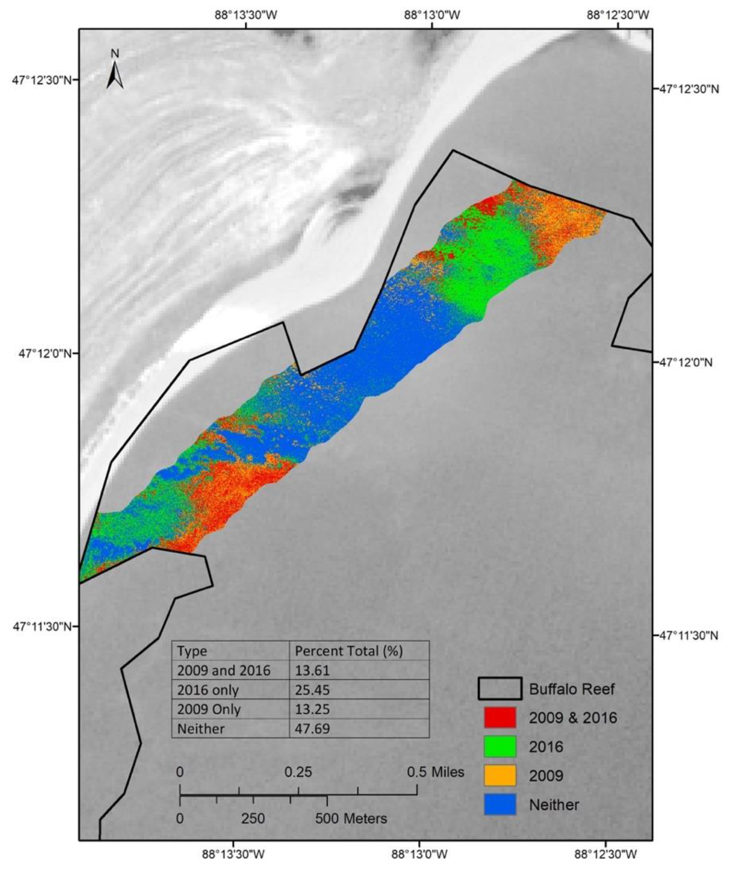[48]. In the end, the strips across the critical region of Buffalo Reef not only verified but also quantified stamp sand encroachment into the northern cobble/boulder fields. Differences between 2009 and 2016 classifications were used for the quantification.

Benthic Sediment (% Stamp Sand and Cu Concentrations). In addition to stamp sand cover, information on substrate copper concentrations was vital to determining ecosystem bottom impacts. To gain more insight, in 2012–2013 and again in 2016–2017, USACE ERDC-EL and MTU jointly sampled sediments across Grand Traverse Bay (Figure 5, left) to aid efforts in sediment transport modeling, determine the distribution and abundance of stamp sand percentages and to directly measure Cu concentrations. Additional Ponar sediment sampling was carried out through vessel investigations in 2016–2017.

Ponar samples were initially taken from the R/V Polar, R/V Agassiz and R/V Sturgeon. Site sampling for sediments included three cruises in August 2012, two cruises in May 2013 and three cruises in June 2013. Later cruises were in September and October of 2016 and spring of 2017. Complementary activities included side-scan and down-scan sonar, Satlantic profiles at multiple stations and ROV underwater filming at numerous sites (Figure 5, right).

Stamp sands at the Gay pile have been characterized by several methods (Neutron Activation and ICP Mass Spectrometry [4,49]; AA [50]; ICP Mass Spectrometry [51]). Early studies of copper concentrations in Gay coarse stamp sand found values ranging between 1620–5486 µg g⁻¹ (mean 2697 µg g⁻¹, n = 7 [4,10], whereas more recent sampling studies by MDEQ [51] on the Gay tailings pile found Cu concentrations 1500–13000 µg g⁻¹ (mean 2863 µg g⁻¹; n = 274). We used the MDEQ pile values here as an initial standard (100% stamp sands = 2863 µg g⁻¹) and predicted potential Cu concentrations in sand mixtures from % stamp sand values.

Later sampling followed up with direct Cu concentration determinations, allowing construction of a field % stamp sand versus Cu concentration calibration curve (see Results). Sediments were digested at MTU in a microwave (CEM MDS-2100) using EPA method 3051A. Solutions were shipped to White Water Associates Laboratory for final analysis. Copper was measured using a Perkin-Elmer model 3100 spectrophotometer. Digestion efficiencies were verified using NIST standard reference material Buffalo River Sediments (SRM 2704) and instrument calibration was checked using the Plasma-Pure standard from Leeman Labs, Inc. Digestion efficiencies averaged 104% and the calibration standard was, on average, measured as 101% of the certified value.

3. Results

3.1. Comparison of Sonar Versus LiDAR Bathymetric Features of Grand (Big) Traverse Bay

Between 1900 to 1932, company records document that two stamp mills (Wolverine and Mohawk Mills) sluiced 22.7 million metric tons (MMt, = Terra-grams, Tg) of copper-rich “stamp sands” onto a tailings pile (“original pile”) off the town of Gay [12]. As a cross-check, Babcock and Spiroff [52] recorded 22.6 MMt of mill rock were crushed. A detailed CCIW RoxAnn Sonar Survey of Buffalo Reef in 2005 shows the basic bathymetric features of Grand Traverse Bay at 4 m intervals (Figure 6, top). Compare the conventional, sonar-derived bathymetric landscape with the 2010 NOAA LiDAR-derived DEM (Digital Elevation Model; Figure 6, bottom). Both indicate the prominent, central position of Buffalo Reef. However, the LiDAR image distinguishes several important finer-scaled bathymetric features. To the northeast, large underwater stamp sand (tailings) bars (#1) move out from the primary pile and stamp sand-covered beaches, migrating across the Jacobsville Sandstone bedrock shelf, coalescing and depositing stamp sand into a channel (“trough” #2) just northeast of Buffalo Reef. Apparently, the “trough” marks an ancient river bed scoured 3 km from near the Coal Dock site through Jacobsville bedrock to a depth of 2–3 m [12,17]. LiDAR shows that stamp sand has mounded up in the northern regions of the “trough” (#3) and is now over-flowing westward into the northern cobble fields of Buffalo Reef (#4). Stamp sand, perhaps originating from the shoreline beach, is also found in a depression west of Buffalo Reef (#5) and east of the Traverse River Seawall (#6).

The LiDAR DEM also emphasizes the difference between the bedrock (Jacobsville Sandstone) rises of Buffalo Reef (#7) and the variety of cobble/boulder beds spreading out around the reef’s core (#8, # 9). The horizontal fields of cobbles and boulders, interspersed with natural sand patches, is what makes Buffalo Reef such an important breeding site in Lake Superior. Natural sand is abundant in the lower bay (#10), forming an almost continuous layer covering bedrock. The sand moves out towards Keweenaw Bay under the influence of long-shore currents, creating a series of natural shallow channels (#11). Bedrock again appears along the shoreline of Traverse Point (#12). Many smaller details are also evident, like the irregular ridges marking the Jacobsville Sandstone bedrock, a canyon-like gap (former fault line?) coursing through the slightly displaced middle of Buffalo Reef and the intertwined rope-like character of the underwater migrating stamp sand bars.

The Gay pile (see NOAA 2010 LiDAR, Figs 6, bottom; Figure 7) was subject to erosion from wave action and prevailing southwestward currents that run parallel to isobaths [37,53,54]. Measurements by Sloss and Saylor [53] documented periodically strong (1.0–5.0 cm s⁻¹) summer and fall southwestward alongshore currents. Nippising beach ridges [55] extend from the Coal Dock to the southern portion of the bay, emphasizing a prolonged depositional history in the lower bay prior to the release of tailings. Narrow white beaches originated around the Coal Dock location, extended southwest to the Traverse River and wrapped around the western lower margin of the lower Bay. From 1901 to the present, stamp sand was redeposited along the beach margin, stretching now down to the Traverse River Seawall. Unfortunately, stamp sands are now seriously over-topping that structure, jeopardizing the lower bay.

From eight georegistered aerial photographs, beach recession at the Gay tailings pile was estimated by calculating meters of shoreline lost each year along four transect lines across the middle portion of the original pile [12]. Based on these measurements, yearly recession has remained nearly constant through time (Y = −7.86X, R² = 0.990), around 7.9 m yr⁻¹ (ca. 26 feet yr⁻¹) through 2016.

Estimating mass erosion from the Gay pile was complicated by original pile depths increasing out into the bay. However, LiDAR revealed the depth of the bedrock surface under removed stamp sand. Using a 1906 bathymetry map, aerial photographs and the 2008 LiDAR bathymetry profiles [12], the mass of stamp sand in million metric tons (MMt) remaining on the pile was estimated through time (Figure 8). The best regression fit is an exponential decay function (Y = 7.646 × 10 ¹⁶, e^−X/53.82 − 1.42), where X is in calendar years; R² = 0.993). Logarithmic transformation creates a linear regression fit (n = 8 points; ln Y = −0.01978 X + 41.1879, R² = 0.993), which estimates a zero intercept of 2082, with 95% confidence intervals between 2077–2091, if mass erosion continues along historic trends.

Annual erosion loss from the tailings pile declined rapidly through time as the pile area and depth diminished, moving from an estimated 356,920 tons/yr in 1938–1939 to 74,200 tons/yr in 2015–2016. Figure 8 (black and red squares) and

Table 2. Area and percentage of beach stamp sand lost, 2008 to 2016 (LiDAR).

Location	Year	Area (ha)	Percent Loss from 2008 to 2016 (%)
Gay Pile	2008	31	19
	2016	25
Shoreline: Between Gay pile and Coal dock	2008	95	3
	2016	92
Shoreline: Coal Dock to Traverse River	2008	41	2
	2016	40

include recent estimates of area and volume eroded and deposited along the shoreline between the 2008–2016 LiDAR overflights. Over time, a little less than half the Gay pile material has been redeposited along the shoreline southwest from the pile, creating a “black sand” beach that extends to the Traverse River Seawall, whereas a little more than half has moved underwater into the bay. The long-term progression of shoreline deposition of stamp sand from aerial photographs (1938–2016) is reconstructed at a MTRI website (http://spatial.mtri.org/stampsands/). The stamp sand beach is now 3–5 times wider and much deeper than the original white beach. Redeposited stamp sands just south of the pile, in the “pond” region, cover more area than the remaining Gay pile (Figure 9 and Figure 10). Stamp sands almost completely surround the Coal Dock and are moving into wetland margins. At the Traverse River, stamp sands are moving across house and cabin lots.

In similar fashion, using the 1906 bathymetry map, aerial over-flight data and 2008 LiDAR contours, we estimated the mass of stamp sand accumulating along the beach margin. Mass accumulation of redeposited “black sands” along the shoreline was nearly linear for 70 years (Figure 8, Y = 0.07 X − 133.15). From the Gay pile to the Coal Dock, accumulation over time (Region 2, 4.5 Tg) also followed a simple linear function (slope = 0.035 X, S.E. = 0.003; R² = O.93). From the Coal Dock to the Traverse River, less material was redeposited (Region 3, 2.6 Tg), following a linear function with a nearly identical slope (slope = 0.035 X, S.E. = 0.001; R² = 0.99). Comparing the mass remaining on the Gay pile to that along the beach in 2010, the shoreline total was double the amount left on the pile (Figure 8, 7 Tg versus 3.4 Tg). However, over time the primary source of eroding stamp sands into the bay began to shift from the Gay pile to the redeposited beach stamp sands (Figure 9; Table 2).

We used the difference between the 2008 to 2016 LiDAR over-flights to calculate recent losses and gains. By 2016 (Figure 10), the greatest amount of tailings along the shoreline includes the remnant of the original pile (2.4 Tg) plus the amount from the pile to the Coal Dock (3.8 Tg), a total of 6.2 Tg. Between 2008–2016, in terms of area, the greatest erosion loss was off the original Gay pile (Figure 9; Region 1), as the area reduced from 31 to 25 ha, a 19% loss, whereas between the Gay pile to Coal Dock (Region 2), the decline was from 95 ha to 92 ha, a 3% loss. Between the Coal Dock to Traverse River Seawall (Region 3), there was a decline from 41 ha to 40 ha, a 2% loss. Thus, the area and volume of shoreline stamp sand along the beach is no longer increasing but is characterized by a net loss. Corresponding regional mass reductions during the 8-year interval (2008 to 2016) are 3.14 to 2.42 Tg (0.72 Tg; ca. 90,000 metric tons/yr) at the Gay pile (Region 1), 4.55 to 3.83 Tg (0.72 Tg; ca. 90,000 metric tons/yr) from the Gay pile to Coal Dock beach region (Region 2) and 2.52 to 2.35 Tg (0.17 Tg; 21,250 metric tons/yr) from the Coal Dock to Traverse Seawall stretch (Region 3). That is, over the 8-year interval of detailed LiDAR data, a net additional 1.61 Tg (201,250 metric tons/yr) moved underwater into the bay. These shoreline sources are contributing to the migrating underwater stamp sand bars, making underwater bar movement dominate temporal dynamics out in the bay.

3.2. Migrating Tailings Encroach Upon Buffalo Reef

In the middle of the bay, Buffalo Reef covers 9.2 km² and is a key breeding ground for lake trout (Salvelinus namaycush) and lake whitefish (Coregonus clupeaformis). The Reef is recognized in the Atlas of Spawning and Nursery Areas in the Great Lakes, Volume 2 [56]. The Lake Superior Biodiversity Conservation Assessment report [57] treats Buffalo Reef as a valuable breeding site for lake trout and whitefish commercially exploited in Keweenaw Bay by Wisconsin (Bad River, Red Cliff) and Michigan (KBIC) tribes. The Great Lakes Indian Fish and Wildlife Commission (GLIFWC) conducted fisheries assessments on the reef between 1986 and 2002, confirming that it is an important spawning reef for lake trout and whitefish [16]. Lake trout were more abundant in the deeper regions, whereas lake whitefish were more common in the shallower, inshore regions. The reef is important because cobble and boulder spawning fields extend over such large areas north, west and south around the bedrock rise. After hatching, lake trout move into deeper waters, whereas lake whitefish from Buffalo Reef use the lower, white-beach portion of the bay as a rearing ground, consuming benthic and pelagic invertebrates as food resources [16].

Because Lake Superior waters are so clear, light penetrates down to the extensive cobble and boulder fields scattered around Buffalo Reef, promoting periphyton (aufwuchs) growth on the rocks (Figure 11, top). Many of the rocks in the cobble/boulder fields are glacial erratic boulders, left when finer-grain sediments were removed by wave action. Although heterogeneous rocks, the rounded cobbles all appear uniformly light greenish-grey, due to the diatom/bacterial cover. Under wave and current action, periphyton continually sloughs off rock surfaces, onto bottom sediments and around reef edges. Wave and current action also moves periphyton particles off the reef and along-shore, enriching benthic food-webs but contributing to suspended matter in the water column. Unfortunately, stamp sand is mounding up in the “trough” and moving westward as extensive fields with ripples, encroaching onto northern cobble field edges and burying rocks (Figure 11, bottom left, right). The underwater stamp sand bars originate from the Gay tailings pile and redeposited stamp sand beach stretch between the Gay pile and the Coal Dock (Regions 1 and 2; Figure 6, bottom). The western portion of the bars is moving over the Jacobsville Sandstone bedrock, dropping into the northern and middle regions of the “trough.” More eastern portions may eventually move off the shelf edge into deeper waters. Clearly, accumulation of stamp sands in the ancient riverbed protected Buffalo Reef for decades, but now is a serious source of concern.

3.3. Hydrodynamic Model Predictions of Stamp Sand Deposition On Buffalo Reef

Ten-year ERDC-EL hydrodynamic predictions [37] of stamp sand deposition are shown in Figure 12. ERDC-EL model sedimentation differences in Grand (Big) Traverse Bay ranged from maximum erosion of −30 inches (−76 cm, red) to positive deposition of +54 inches (+ 137 cm; purple). Yellow to red regions indicate pronounced net erosion along the Gay Pile and Gay Pile to Coal Dock stretch (Regions 1 and 2; right red, brown and yellow zones). Green to dark blue regions mark net deposition, emphasizing three major regions of accumulation: 1) northern portion of the “trough,” extending into the northern boulder fields of Buffalo Reef (Figure 12, location #3); 2) middle and southern portions of the “trough” (location #4), where stamp sands are starting to move around the southern fringe of Buffalo Reef; 3) west of the Buffalo Reef bedrock high, corresponding to the western depression (Figure 6, location #5) and merging with material east and south of the Traverse River Seawall. There is also beginning accumulation west of the Traverse River Seawall along the white sand beach. Moreover, the model predicted that, without mitigation action, an estimated 60% of Buffalo Reef would be covered by at least 1 inch (2.5 cm) of stamp sand over the next 10 years.

Using 2008–2013 LiDAR as benchmarks, on an annual basis, the ERDC-EL conceptual site model (CSM) suggests ca. 50,000 m³ (82,500 tons; using the 1.65 tons/m³ conversion) of stamp sands would be eroded from in front of the main pile. Most material (ca. 42,000 m³; 69,300 tons) would be transported in the long-shore (i.e. down-drift) direction along the beach margin, with about 8,000 m³ (13,200 tons) transported offshore, largely during high-energy events (major storms). Approximately 23,000 m³ (37,950 tons) of the eroded sediments transported long-shore would end up in the trough, whereas ca. 6,100 m³ (10,065 tons) would be transported onto Buffalo Reef. The remainder (13,000 m³; 21,450 tons) would be transported long-shore towards the Traverse River Seawall. The small particle size-fraction (7–14%) of the sediment (e.g., slime-clay component) that is initially transported onto Buffalo Reef would get resuspended and transported further offshore during subsequent major storm events, ending up contributing to the “halo” around the Keweenaw Peninsula. Eventually the amount of tailings that gets transported onto Buffalo Reef from the Gay pile will diminish with time as the up-stream sources dwindle.

3.4. Bottom Reflectance Estimations of Stamp Sand Cover on Buffalo Reef

How do the ERDC-EL 10-year predictions (60% cover) coincide with recent stamp sand cover on Buffalo Reef? Figure 13 shows the substrate classification for 2009 based on the 3-band NAIP survey. Superimposing the outline from Buffalo Reef over the image provides an estimate of ca. 25% cover by stamp sand (red). However, the deepest portions of Buffalo Reef are not covered within boundaries, as bottom reflectance was not adequate. Comparing the 2009 NAIP map (Figure 13) with the ERDC-EL deposition map (Figure 12), there are two major areas of stamp sand incursions: one northern region out of the “trough” and a western region in a depression off the bedrock rise (see Figure 6, site #5). The latter merges with the region south of the Traverse River Seawall. Thus, stamp sand cover (red) compared favorably with the ERDC model results.

In Figure 14 we cross-compare substrate maps based on the 2009 3-band NAIP, 13-band 2016 Sentinel-2 and 288-band 2016 CASI. Here grey color within the boundary of the top two figures indicates deep-water regions where no bottom reflectance could be recovered, that is, regions of uncertainty. In the 13-band Sentinel-2 (Figure 14, middle), stamp sand cover increases to 35% cover. Moreover, the Sentinel-2 images of 2016 stamp sands around the western Seawall show greater dispersal, that is stamp sands scattered over a greater area and also indicate a slight southward shift around the Seawall. However, the Sentinel-2 substrate map also suggests stamp sand ringing the southern and southwestern deep-water margins of Buffalo Reef. We will later discover (from Ponar % stamp sand particle counts) that the deep-water indication of stamp sand around Buffalo Reef is probably in error, that the two sand end-members could not be differentiated in deep waters. In shallow water, the 288-band CASI strip (Figure 14, bottom) conformed reasonably well to both the northern NAIP and Sentinel-2 bottom classifications. In Figure 14, cobble fields (yellow) were rather uniformly colored, despite heterogeneous rock composition, probably due to the similar color of aufwuch-coated periphyton. Although the hyperspectral CASI substrate classifications could not precisely differentiate % stamp sand in mixed sand end-members, they were sufficient to indicate relative expansions of stamp sand cover.

Differences between the 2009 NAIP and 2016 hyperspectral bottom classifications suggested active movement of stamp sands onto Buffalo Reef (Figure 15). Areas shown in red were classified as stamp sands in both 2009 and 2016. Areas in green were stamp sands in 2016. Areas in orange were stamp sands present only in 2009. The blue areas represent areas where stamp sands were not identified in 2009 or 2016. The figure highlights areas of good agreement (red) between the 2009 and 2016 images. However, there were areas of increasing stamp sand cover in the image difference strip. An overall 12% gain of stamp sand occurred along the image strip, in two regions (eastern out of “trough,” western southward from Traverse River shoreline), the latter where stamp sands moved westward ca. 200–300 m. Spatial comparisons of bottom classifications and ground-truth measurements are given in

Table 3. Matches between reflectance-derived substrates and ground-truth observed substrates. Observed substrates are based on a combination of Ponar plus ROV ground-truth sites.

Observations	Total	Match	Mis-match	% Match
A. Shallow-water (0-8m)
2009 NAIP	35	33	2	94%
2016 Sentinel-2	68	54	14	79%
2016 CASI	44	41	3	93%
B. Deep-water (8-14m)
2016 Sentinel-2	68	22	46	32%

. In shallow water (0–7m), comparisons are good (79–94% agreement), whereas in deep water (8–14m), comparisons are poor (<40% agreement).

3.5. Direct Estimations of Stamp Sand Cover (%Stamp Sand; Copper Concentrations)

Because the sources of sands are so distinct (crushed basalt, from the Portage Lake Volcanics; versus rounded quartz from eroding Jacobsville Sandstone, see Methods), stamp sand percentages could be approximately determined from Ponar sediment grab samples. Stamp sand percentages from around 90 sites are plotted in Figure 16. Along the shoreline, percentages of stamp sand are highest off the primary Gay pile and along the redeposited stamp sand beach margin up to the Coal Dock, forming a strip of values 0.5–0.75 km wide. Based on % stamp sand composition, anticipated Cu concentrations are relatively high in the nearshore region, 1,717–2,860 ppm (Figure 16). Percentages decline (to 30–10%) off the Buffalo Reef bedrock ridge intersection with the shoreline, then increase back to half (40–60%) towards the Traverse River Seawall location. As one moves 2-4 km offshore from the beach, stamp sand percentages decrease to about 21–11% (573–287 ppm). One can overlay the outline of Buffalo Reef on a map of % stamp sand and calculate the % area on Buffalo Reef covered by >20% mixture of stamp sands. The procedure indicates ca. 35% of the Buffalo Reef area is covered by stamp sands, a value similar to the Sentinel-2 findings. This operation provides a third, independent, estimate of stamp sand cover on Buffalo Reef, one that covers the entire reef.

However, direct counts of grains suggest little accumulation of stamp sands around the southern margins of Buffalo Reef, a serious difference with the Sentinel-2 substrate map (Figure 16). Reductions of stamp sand percentage offshore reflect greater distances from primary sources (original pile; stamp sand beach deposits) plus active mixture with migrating natural sands, that is, dilution effects from mixing. As stamp sands move into the southern bay region, where natural sands are much more abundant, we would predict even more mixing of natural and stamp sands and more dilution.

When the % stamp sand map is translated into copper concentrations, coastal toxic effects on biota would be expected to be severe. A copper calibration curve, based on observed Cu concentrations in Ponar samples versus predicted values from % stamp sand grain counts, gives a regression equation of Y = 1.002 X − 220; R² = 0.911, with a linear regression ratio of almost equal slope (1.00). Even with some chelation from humic water discharge (river mouths), at Cu concentrations of 400–700 µg/g or higher there should be serious toxic impacts on benthic biota [13,58,59].

4. Discussion

LiDAR & Reflectance Studies. The combination of LiDAR and bottom reflectance imagery, plus ground-truth measurements, is greatly improving substrate classification accuracy and coastal modeling studies [60,61]. Substrate reflectance imagery and LiDAR combinations have been used in studies of coastal estuaries [62], coral reefs [61] and mining studies [63]. Here five LiDAR (2008, 2010, 2011, 2013, 2016) over-flights greatly improved ERDC-EL hydrodynamic models [29] and clarified key features of the coastal landscape. Bottom reflectance studies helped quantify movement of stamp sands across the bay and onto Buffalo Reef. In particular, the 2008–2016 LiDAR over-flights of the bay complemented by reflective imagery (3-band NAIP; 13-band Sentinel-2, 48-288 band CASI multispectral and hyperspectral), along with ground-truth Ponar and ROV studies, allowed up-to-date quantification of tailings erosion and deposition along the coastal beaches and documented the whereabouts and movements of stamp sands (tailings) underwater in the bay. 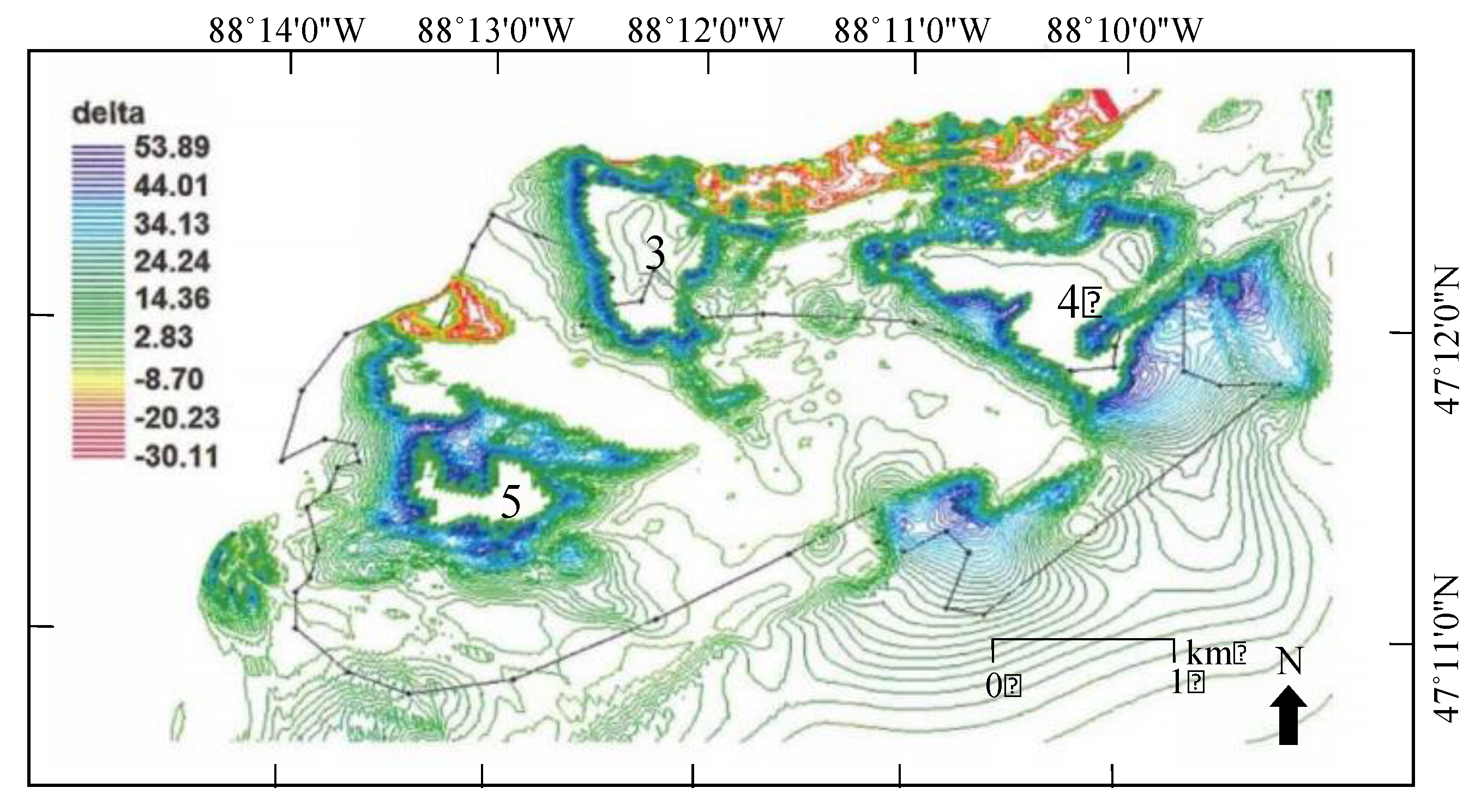Moreover, the multiple LiDAR bathymetric characterizations provided invaluable detailed information that aided modeling particle movement and spatial sedimentation patterns (Figure 12; [29]). LiDAR and MSS imagery showed that the “trough,” an ancient riverbed cut just up-drift of Buffalo Reef, originally collected migrating bars of stamp sands and previously protected the reef.

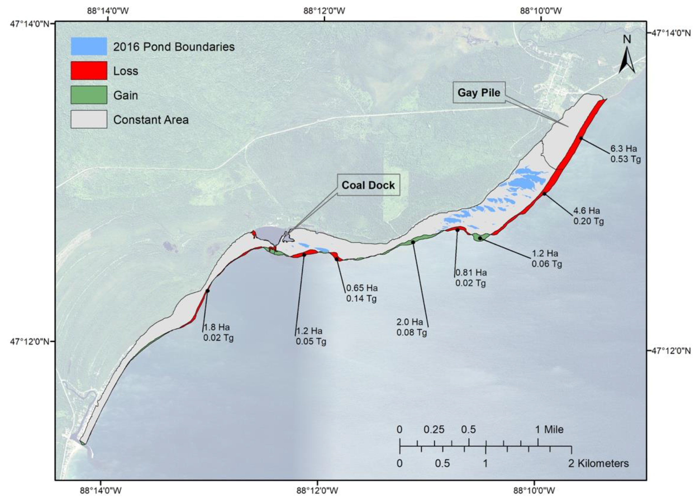
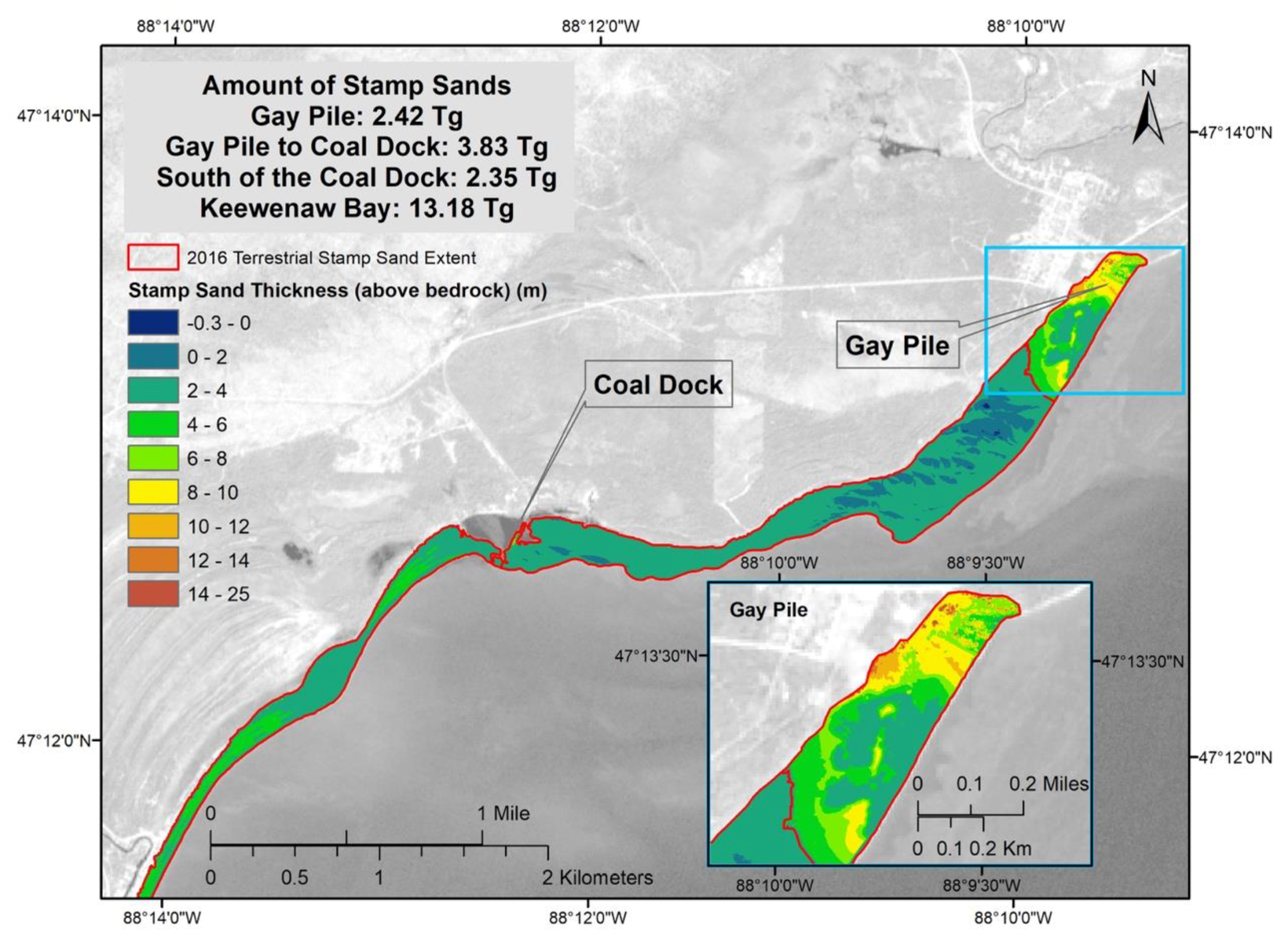
Annual calculations from aerial photos and recent LiDAR over-flights have quantified tailings eroding from the main pile and depositing along the shoreline as extensive beaches. Recent over-flights estimated 75,700 metric tons eroding from the Gay pile in 2014–2015, close to the ERDC-EL model estimate of 69,150 tons/yr. ERDC also predicted 30,960 tons/yr deposited into the “trough” and 8260 tons/yr of stamp sands moving into the boulder fields [29,64]. Hydrodynamic modeling by ERDC-EL predicted that if nothing were done, 60% of Buffalo Reef would be covered by stamp sands within the next 10 years (Figure 12).

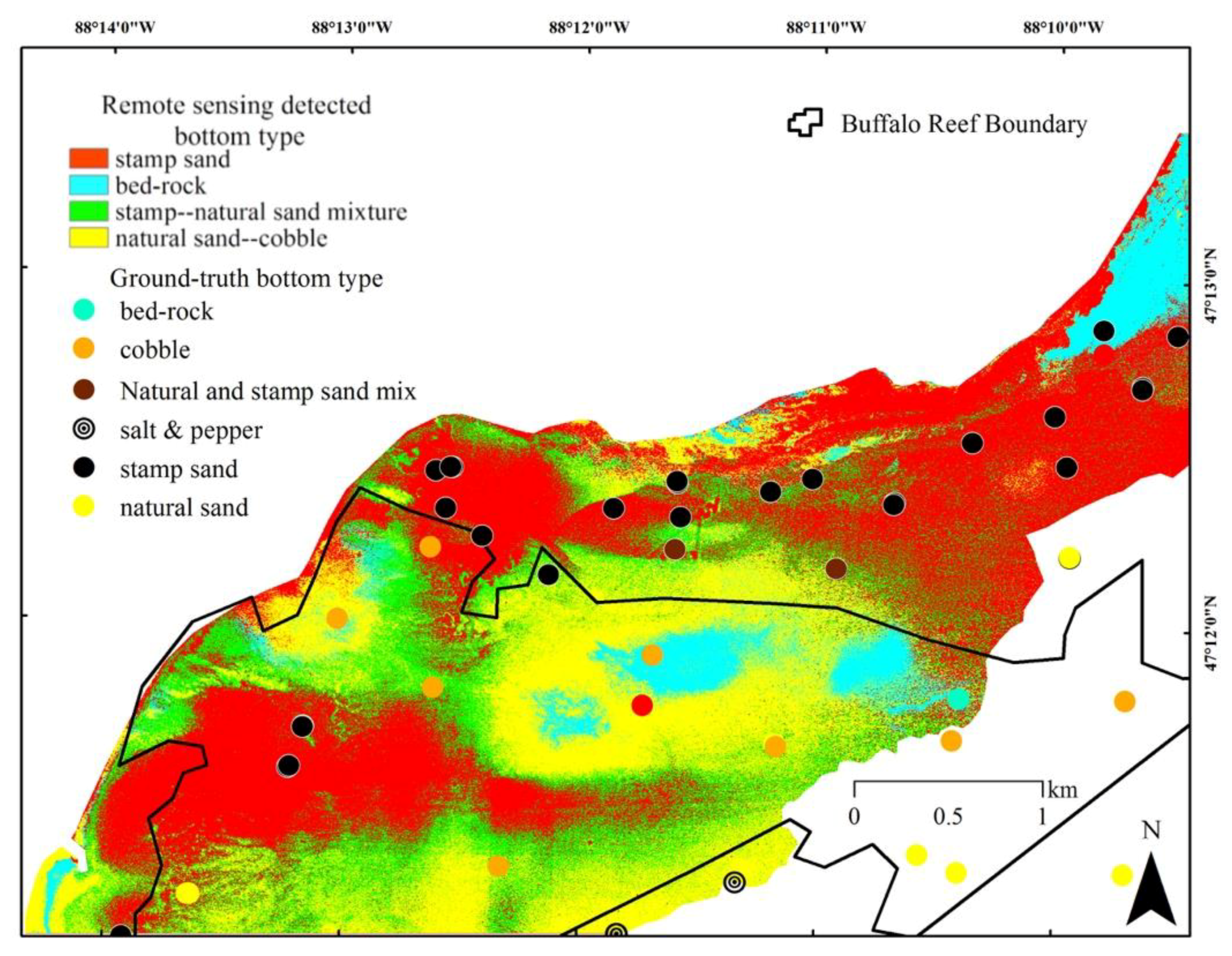
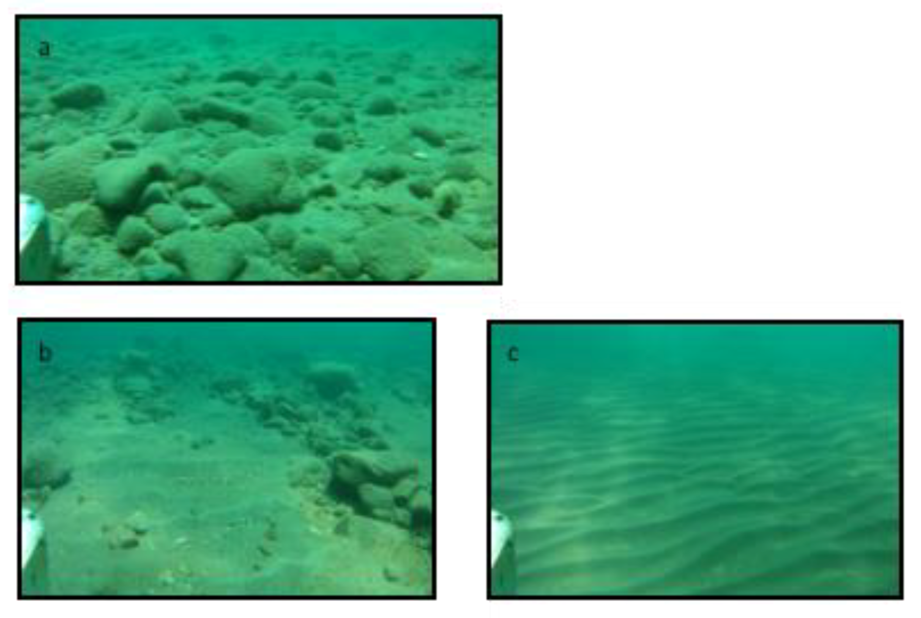
Spectral reflectance differences in 2009 (NAIP studies) suggested good shallow-depth resolution of three primary substrate types along the coastal margin: stamp sands, natural beach sands and Jacobsville Sandstone bedrock [12]. Ponar and ROV studies showed good matches between NAIP-derived substrate classifications and observed site substrates (Figure 14; Table 3). Here we relied upon bottom reflectance studies to estimate how much of Buffalo Reef has been covered by tailings (stamp sands) between 2009–2016. Reflectance imagery (3-band NAIP, 13-band Sentinel-2, 84-band CHARTS CASI) permitted updated estimates of Buffalo Reef area covered by stamp sands, showing that cover had increased from 25–27% (2009) to around 35% (2016), that is, better than 50% towards the ERDC-EL 10-year predictions. ROV and Ponar sampling confirmed the migrating front of stamp sands and the high concentrations of copper in the migrating sands. Underwater photography (ROV studies) showed that high concentrations of stamp sands were killing biologically active photosynthesizing layers (aufwuchs) on cobbles and boulders, were toxic to benthic invertebrate communities and were burying entire cobble fields [14,64].

Although remote sensing technologies have improved studies of coastal shelf margins, extracting and interpreting data from aerial over-flights and orbital satellite platforms remains complicated. One of the serious problems encountered involved photons directly or diffusely reflected by the air-water interface according to Fresnel laws. The spectral reflection of direct sunlight contributes to what is commonly referred to as the “sunglint” effect. The amount of energy reflected by the surface depends upon sea state, wind speed and observation geometry (solar and view angles). In images with very high spatial resolution (<10 m), sunglint causes a texture effect that introduces bottom confusion and distortions in reflectance spectrum [48,65,66]. In our shallow-water CASI hyperspectral applications, attempts were made to overcome sunglint effects. After correction, the CASI substrate classification handled some of the stamp sand and natural sand end-member mixture problems. The detailed CASI strip-analysis not only resembled earlier substrate classification maps but difference comparisons suggested 250 m more westward encroachment by stamp sands into the northern boulder fields of Buffalo Reef since 2009. However, attempts to extend shallow-water bottom reflectance classifications deeper, off the southern margins of the reef, encountered several additional problems.

Relative to excellent spatial coverage of Buffalo Reef by LiDAR, both NAIP and Sentinel-2 passive color reflectance efforts were severely limited by water depth. Natural depth penetration of solar radiation and bottom reflectance was much less than the 20–22m depth repeatedly achieved by LiDAR. Passive light penetrated down only to 7–8 m with reliable spectral retrieval. The total area of Buffalo Reef was 9.2 km², whereas the area visible on both bottom reflectance maps was only 4.83 km², around 52% of the total reef area. In shallow waters, because of major albedo differences between stamp sands and natural sands, “mixed stamp sand” substrates did show good bottom reflectance gradients and mixtures of the two end members were handled fairly well in 3-band NAIP and CASI hyperspectral applications. Cross-comparisons of shallow-water spatial substrate classification maps for 2009 NAIP, 2016 Sentinel-2 and 2016 CASI multispectral-hyperspectral image strips produced very similar results (Figure 14). However, in deeper-water substrate maps, there were slight spatial misclassifications in the 2009 NAIP data but serious errors in Sentinel-2 maps (Table 3). Although 2016 Sentinel-2 images had stamp sand regions covering 33–35% of Buffalo Reef, similar to final Ponar direct particle count estimates, yet the processed image indicated stamp sand presence around the deeper southern margins of Buffalo Reef, a feature not found in direct particle counts.

Specifically, direct grain counts from Ponar samples suggested that Sentinel-2 imagery incorrectly indicated stamp sands ringing the southern and deep southwestern edges of Buffalo Reef. Application of the basic Lyzenga transformation to deep-water class-2 coastal waters probably was responsible for some of the deep-water local misclassification errors, similar to difficulties others have encountered in classifying Florida coast and coral reef substrates in deeper waters [61,67,68]. However, numerous in situ spectral radiance and irradiance profiles (Satlantic OC P1000 Optical Profiling Radiometer) allowed us to investigate the potential causes of the unwanted variance and misclassification. Several well-known uncertainties may cause increasingly large biases in retrieving deeper-water bottom reflectance.

A significant problem in the use of multispectral to hyperspectral data for benthic mapping is that perturbations to airborne radiance caused by water depths and water column attenuation are not easily decoupled from changes in radiance caused by changes in bottom reflectance. All reflectance models are based on the exponential decay of light and reflectance from deeper bottom surfaces enhances uncertainties. Moreover, in the first meters of the water column, environmental factors such as waves, bubbles, stratification and fluctuations of the surface can introduce noisy patterns [68,69,70], whereas spatial differences from dissolved or suspended materials (DOC, phytoplankton, zooplankton) may complicate albedo and irradiance calculations. At deeper depths, it is difficult to accurately retrieve bottom reflectance because of differential exponential light absorption by water, plus scatter by suspended material and organisms [71]. Sample down-welling data from Satlantic casts (Figure 3, bottom right) show how photons from longer (red, yellow) wavelengths are severely curtailed with depth, favoring the blue-green wavelengths used in coastal LiDAR. We examined Satlantic casts from numerous sites in the bay (Figure 5, right) performed around the 2009 NAIP and 2016 CASI and Sentinel-2 over-flights dates. Data on bottom return spectra from depths greater than 8m clearly show severe spectral attenuation of longer and shorter wavelengths, plus the loss of albedo differences between natural and stamp sand substrates (Figure 17). Blue and green-band spectra from passively bottom-reflected surfaces also become highly variable at the surface.

Lyzenga’s algorithm [46,65] was one of the earliest depth-correction algorithms and requires relatively little field data from the water column for application. For this reason, it is by far the most frequently applied. However, clear waters are a necessary prerequisite for accurate application. Here we deal with application to coastal case-2 waters, with increased dissolved compounds (DOC), suspended material and organism (phytoplankton, zooplankton) concentrations that both absorb and scatter light in deeper water columns. Below 8m depth, Lyzenga’s algorithm applied to Sentinel-2 data produced spurious pixel values (Table 3). Depending on depth and K_d, it is not always possible to retrieve a bottom signal or the retrieved signal may be subject to a great degree of uncertainty. In particular, Buffalo Reef appears compromised by periphyton sloughing off cobbles and boulders and by greater concentrations of plankton ringing the deep-water margins. Depth issues with bottom reflectance are commonplace. Mumby et al. [72] applied a simple model to correct a CASI image of French Polynesian marine water values. Their model only considered the reflectance at the surface (ρ_w), K_d and depth for each point of the image and bottom reflectance was obtained as ρ_b = R_we^−Kdz. The K_d was obtained by the same approach as Lyzenga’s method, by using the slope of the natural logarithm of reflectance for a uniform substratum (sand) against the depth from ground-truth maps. Model performance did not include corrections for additional water column effects (suspended sediment, DOM, phytoplankton). Leiper et al. [71] suggested a physics-based inversion method with Hydrolight and ENVI software, yet still found that, in waters deeper than 8 m, the match between the classified image and field validation data was poor. Clearly, depth effects in bottom reflectance studies remain a very active area of research.

Geographic Incidence of Coastal Mine Tailings Releases. The Keweenaw Peninsula is not unique. There are numerous examples of intentional and unintentional mine tailing releases into coastal freshwater and marine environments. In several regions, such practices are now unlawful, for example, the 1972 Clean Water Act of the U.S. and Canada banned tailings discharge into coastal waters of the Laurentian Great Lakes. However, many earlier discharges, such as those at Gay, fall under a “legacy” category, that is, occurring prior to regulation. Moreover, in 2012–2013, global marine and freshwater (river) disposal of tailings was conducted by 18 mines (4 into rivers, 14 into marine waters) and most by metal operations (copper, gold, silver, iron and rutile mines; [8]).

“Unintentional” contributions include periodic tailings dam failures that release large volumes of slurries into fresh or marine coastal waters [73,74]. An estimated 3500 mine tailing impoundments/dams exist worldwide [8]. Recent regional tallies include: 839 tailings dams in the United States (USACE & UNESCO), 350 impoundments in Western Australia, 65 in Quebec and 130 in British Columbia, Canada; 400 in South Africa; and 500 in Zimbabwe [75]. Along the Mediterranean coast, there are over 230 tailings dams in the Spanish Province of Almeria alone, some dating back to Roman times [73].

Biological Effects of Tailings on Food Webs. Stamp sands at the Gay pile have been characterized numerous times. Early determinations of Cu concentrations in the Gay pile coarse stamp sand ranged between 2750 to 3250 µg g⁻¹ (mean 2959 (SD 121) µg g⁻¹, n = 29, [76]), 1620 to 5486 µg g⁻¹ (mean 2697 µg g⁻¹, n = 7; [4,9]), whereas more extensive sampling efforts in 2003 by the Michigan Department of Environmental Quality [77] found Cu concentrations ranging between 1500–13,000 µg g⁻¹ (mean 2863 µg g⁻¹; n = 274). Additional important metals in a secondary suite included: Al (mean 15,872 µg g⁻¹), Ag 0.4–7.7 µg g⁻¹ (mean 1.8), As 1.0–15.5 µg g⁻¹(mean 1.5), Cr 18–52 µg g⁻¹ (mean 28.8), Co 16–36 µg g⁻¹ (mean 22.9), Hg 0.06–0.11 µg g⁻¹ (mean 0.027), Mn (mean 549 µg g⁻¹), Ni 20–48 µg g⁻¹ (mean 31), Pb 5.1–6.1 µg g⁻¹ (mean 2.6) and Zn 48–120 µg g⁻¹ (mean 74.7; [51]).

At the original Gay pile site, several metals exceed state Groundwater Surface Water Interface Criteria (GSWIC) levels. In the 274 soil samples, aluminum exceeded levels in 271 samples, chromium in 265, cobalt in 271, copper in 274, manganese in 159, nickel in 168, silver in 216 and zinc in 242. In 10 groundwater samples, the number of metals exceeding GSWIC risk criteria included: chromium 5, copper 10, manganese 5, nickel 8, silver 8 and zinc 8. In 2003, MDEQ also sampled stamp sands from a southern redeposited stamp sand beach site, north of the Traverse River Seawall (n = 24 samples). Copper averaged lower, 710-5300 µg g⁻¹ (mean = 1443 µg g⁻¹). In the 25 samples, various metals again exceeded GSWIC levels: aluminum in 20 samples, chromium in 19, cobalt in 24, copper in 24, manganese in 7, nickel in 8, silver in 9 and zinc in 10 [77].

Concentrations of copper detected in elutriates of Lake Superior nearshore sediments off the tailings pile and southward along the stamp sands shoreline plus from stamp sand pond water samples were above both acute and chronic Rule 57 Water Quality Values [51]. Thus, stamp sand releases metals at concentrations expected to have acute and chronic effects on aquatic organisms in water column boundary layers and in the small, shoreline enclosed ponds. Several tests of sediments off stamp sand piles and specific tests at Grand Traverse Bay have demonstrated toxic effects. Freshly worked stamp sand in lake sediments is toxic to Daphnia and mayflies (Hexagenia) because they release Cu across the pore-water gradient [59]. Additional laboratory toxicity experiments with stamp sand-sediment mixtures at EPA-Duluth [58,78,79] showed that solid-phase sediments and aqueous fractions (e.g., interstitial water) were lethal to several taxa of freshwater macroinvertebrates: chironomids (Chironomus tentans), oligochaetes (Lumbriculus variegates), amphipods (Hyalella azteca) and cladocerans (Ceriodaphnia dubia). The observed toxicity was due almost exclusively to copper, not to other metals in the secondary suite (principally zinc and lead). Weston’s [51] studies of toxicity in Grand Traverse Bay utilized Ceriodaphnia dubia, Hyalella azteca and Chironomous dilutes with five sediment samples from the Gay pile and the southward stamp sand shoreline. All sediment samples showed acute and chronic effects (growth) on benthic organisms. In more recent MDEQ investigations [80], six sediment locations were sampled along the Gay to Traverse River shoreline transect. Copper concentrations varied between 1500-8500 µg g⁻¹ (mean 2,967), whereas the secondary suite had: Ag 1.2–1.7 µg g⁻¹ (mean 1.5), As 1.7–3.1 µg g⁻¹ (mean 2.2), Ba 6.6–8.6 µg g⁻¹ (mean 7.7), Cr 31–39 µg g⁻¹ (mean 35), Pb 2.1–2.9 µg g⁻¹ (mean 2.6) and Zn 62–79 µg g⁻¹ (mean 72). Bulk sediment toxicity testing showed that all six sediment samples from the shoreline were acutely toxic to both Chironomus dilutes and Hyalella azteca. Two samples taken just south of the Traverse River in a largely white sand bottom also had excessive copper concentrations (300-400 µg g⁻¹), whereas one sample further down the white beach had expected lower concentrations (79 µg g⁻¹).

Recent invertebrate sampling surveys demonstrated severe reduction of benthic taxa where % stamp sand and Cu concentrations were elevated [28]. Using beach seine techniques, GLIFWC has also recently [81] documented that eight YOY species remain relatively abundant in shallow waters off the lower white beach, including lake whitefish, whereas there is a virtual absence of all YOY fishes along the stamp sand beaches from the Gay pile to the Traverse River. Absence of food where stamp sand concentrations are high (i.e. lack of benthic organisms) or high concentrations of copper could both be contributing to YOY fish absence.

Remediation Responses. The Lake Superior Lake Management Plan (LAMP) now considers migrating stamp sands along beach margins as one of their highest priority concerns, relative to contamination of Lake Superior waters. The Great Lakes Indian Fisheries Wildlife Commission (GLIFWC) estimates that collapse of Buffalo Reef could have dire short- and long-term consequences. A preliminary assessment of the fishery by GLIFWC [15], suggests commercial loss of 67,222 kg of lake whitefish and 31,946 kg of lake trout per year, plus 10.4 tribal fishing jobs. Stocking lake trout to replace loses would cost around $380,000/yr. The total loss to commercial and recreational fishing, plus stocking costs, could reach $1,680,000/yr. As a combined consequence of GLIFWC concerns, EPA Great Lakes National Program Office (GLNPO)-sponsored LiDAR/MSS findings (partly reviewed here) and the USACE ERDC-EL modeling, EPA GLNPO appropriated $3.1 M for dredging and planning activities under GLRI (Great Lakes Restoration Initiative) funds. The proposed dredging in 2019 would remove 36,000 yd³ (27,524 m³ = 37,157 tons) of stamp sands from the Traverse River Harbor and 178,000 yd³ (136,091 m³ = 183,723 tons) from the “trough.” In the fall of 2017, the state committed an additional $300K for immediate dredging to protect against “back-up” of river waters if there were serious November storms. Given the estimated yearly deposition into the “trough” (30,960 tons/yr), a one-time removal from the harbor and Buffalo Reef is considered to be sufficient for 3–5 years as a “stop-gap” measure, while planning is underway for longer-term measures.

5. Conclusions and Future Perspectives

Because migrating tailings contributed an end-member with distinctive albedo and spectral features, the combination of LiDAR and passive bottom reflectance greatly aided study of coastal shelf environments impacted by mining discharges in Lake Superior. Within Grand Traverse Bay, migrating copper-rich tailings (22.7 million metric tons) from two stamp mills (Mohawk and Wolverine) are threatening an important lake trout and whitefish breeding ground. Buffalo Reef is a major breeding site for commercial and recreational lake trout and lake whitefish production (32% of the commercial catch in Keweenaw Bay, 22% in southern Lake Superior). LiDAR-assisted hydrodynamic modeling by USACE ERDC-EL (Vicksburg) predicted 60% tailings cover of Buffalo Reef within 10 years, if nothing more was done. Of the substrate end-members, tailings originate from the Portage Lake Volcanic Series and are crushed basalt, with low albedo and spectral signatures different from natural bedrock (Jacobsville Sandstone) and bedrock-derived natural coastal white beach quartz sands.

Multiple CHARTS and CZMIL over-flights between 2008–2016, complemented by ground-truth (Ponar sediment sampling, ROV photography) and passive bottom reflectance studies (3-band NAIP; 13-band Sentinal-2 orbital satellite; 48- and 288-band CASI) helped quantify the topography of the coastal shelf region and mapped details of tailings migration along the shoreline and onto Buffalo Reef. Bathymetric detail from five over-flights was very similar, revealing stamp sand bars migrating from the primary tailings pile and coastal redeposited beach locations and initial deposition of stamp sands into an ancient river bed channel (the “Trough”) northeast of Buffalo Reef, that initially helped protect the reef. Unfortunately, stamp sand has filled up much of the ancient river-bed and is now moving westward across the reef. Substrate mapping challenges around Buffalo Reef featured the physical mixing of two end-members (stamp sands, natural white sands) and water depth-related return of bottom spectral signals, complicating application of the Lyzenga Method.

Passive reflectance cover was much more depth-limited than LiDAR (only 45% coverage) but clearly showed stamp sands moving across Buffalo Reef into cobble breeding grounds. Shallow-water passive bottom reflectance studies estimated 25–35% tailings cover of present-day Buffalo Reef. These results were similar to independent estimates from direct particle counts (~35% cover). However, deep-water (>8m) application of the Lyzenga Method to bottom substrate characterization showed relatively poor matches with ground truth. Poor and highly variable bottom substrate classification probably resulted from a combination of (1) truncated bottom spectral return and (2) increasing water column absorbance by greater amounts of suspended particles (water column plankton, periphyton sloughing off cobble and boulder surfaces) occurring along the deeper edges. To improve matches between LiDAR and bottom-reflectance spectral studies, we recommend development of multiple-color beam LiDAR to extend bottom reflectance examination.

References

1. Cook, P.M.; Glass, G.E.; Tucker, J.H. Asbestiform amphibole minerals: Detection and measurement of high concentrations in municipal water supplies. Science 1974, 185, 853–855. [Google Scholar] [CrossRef] [PubMed]
2. Kemp, A.L.; Williams, J.D.; Thomas, R.L.; Gregory, M.L. Impact of man’s activities on the chemical composition of the sediments of Lakes Superior and Huron. Water Air Soil Pollut. 1978, 10, 381–402. [Google Scholar] [CrossRef]
3. Kerfoot, W.C.; Nriagu, J.O. Copper mining, copper cycling and mercury in the Lake Superior ecosystem: An introduction. J. Great Lakes Res. 1999, 25, 594–598. [Google Scholar] [CrossRef]
4. Kerfoot, W.C.; Jeong, J.; Robbins, J.A. Lake Superior mining and the proposed Mercury Zero-discharge Region. In State of Lake Superior; Munawar, M., Ed.; Aquatic Ecosystem Health and Management Society: Burlington, ON, Canada, 2009; pp. 153–216. [Google Scholar]
5. Benedict, C.H. Red Metal—The Calumet and Hecla Story; University of Michigan Press: Ann Arbor, MI, USA, 1952. [Google Scholar]
6. Lankton, L. Cradle to Grave; Oxford University Press: Oxford, UK, 1991. [Google Scholar]
7. Langston, N. Sustaining Lake Superior; Yale University Press: New Haven, CT, USA, 2017. [Google Scholar]
8. Vogt, C. International Assessment of Marine and Riverine Disposal of Mine Tailings. In Proceedings of the Secretariat, London Convention/London Protocol, International Maritime Organization, London, England & United Nations Environment Programme-Global Program of Action, London, UK, 1 November 2012; p. 134. [Google Scholar]
9. Kerfoot, W.C.; Rossmann, R.; Robbins, J.A. Elemental mercury in copper, silver and gold ores: An unexpected contribution to Lake Superior sediments with global implications. Geochem. Explor. Environ. Anal. 2002, 2, 185–202. [Google Scholar] [CrossRef]
10. Kerfoot, W.C.; Harting, S.L.; Jeong, J.; Robbins, J.A.; Rossmann, R. Local, regional and global implications of elemental mercury in metal (copper, silver, gold and zinc) ores: Insights from Lake Superior sediments. J. Great Lakes Res. 2004, 52, 162–184. [Google Scholar] [CrossRef]
11. Gewurtz, S.B.; Shen, L.; Helm, P.A.; Waltho, J.; Reiner, E.J.; Painter, S.; Brindle, I.D.; Marvin, C.H. Spatial distributions of legacy contaminants in sediments of lakes Huron and Superior. J. Great Lakes Res. 2008, 34, 153–168. [Google Scholar] [CrossRef]
12. Kerfoot, W.C.; Yousef, F.; Green, S.A.; Regis, R.; Shuchman, R.; Brooks, C.N.; Sayers, M.; Sabol, B.; Graves, M. Light Detection and Ranging (LiDAR) and multispectral studies of disturbed Lake Superior coastal environments. Limnol. Oceanogr. 2012, 57, 749–771. [Google Scholar] [CrossRef]
13. Kraft, K. Pontoporeia distribution along the Keweenaw shore of Lake Superior affected by copper tailings. J. Great Lakes Res. 1979, 7, 258–263. [Google Scholar] [CrossRef]
14. Kerfoot, W.C.; Hobmeier, M.M.; Yousef, F.; Green, S.A.; Regis, R.; Brooks, C.N.; Shuchman, R.; Anderson, J.; Reif, M. Light detection and ranging (LiDAR) and Multispectral Scanner (MSS) studies examine coastal environments influenced by mining. ISPRS Int. J. Geo-Inf. 2014, 3, 66–95. [Google Scholar] [CrossRef]
15. GLIFWC. Keweenaw County, Michigan—Gay Stamp Sands: Comments on the proposed GLFER Project. Great Lakes Indian Fish and Wildlife Commission (GLIFWC); Whitepaper; GLIFWC: Odanah, WI, USA, 2012; 8p. [Google Scholar]
16. Chiriboga, E.D.; Mattes, W.P. Buffalo Reef and Substrate Mapping Project; Administrative Report 08-04; Great Lakes Indian Fish and Wildlife Commission (GLIFWC): Odanah, WI, USA, 2008. [Google Scholar]
17. Yousef, F.; Kerfoot, W.C.; Brooks, C.N.; Shuchman, R.; Sabol, B.; Graves, M. Using LiDAR to reconstruct the history of a coastal environment influenced by legacy mining. J. Great Lakes Res. 2013, 39, 205–216. [Google Scholar] [CrossRef]
18. Ackermann, F. Airborne laser scanning-present status and future expectations. J. Photogram. Remote Sens. 1999, 54, 64–67. [Google Scholar] [CrossRef]
19. Banks, K.W.; Riegal, B.M.; Shinn, E.A.; Piller, W.E.; Dedge, R.E. Geomorphology of the Southeast Florida continental reef tract (Miami-Dade, Broward and Palm Beach Counties, USA). Coral Reefs 2007, 26, 617–633. [Google Scholar] [CrossRef]
20. LeRocque, P.E.; West, G.R. Airborne Laser Hydrography: An Introduction. In Proceedings of the ROPME/PERSGA/IHB Workshop on Hydrographic Activities in the ROPME Sea Area and Red Sea, Kuwait City, Kuwait, 24–27 October 1999. [Google Scholar]
21. Abdallah, H.; Bailly, J.; Baghdadi, N.; Saint-Geours, N.; Fabre, F. Potential of space-borne LiDAR sensors for global bathymetry in coastal and inland waters. IEEE J. Sel. Top. Appl. Earth Obs. Remote Sens. 2013, 6, 202–216. [Google Scholar] [CrossRef]
22. Biberhofer, J.; Procopec, C.M. Delineation and Characterization of Aquatic Substrate Features on or Adjacent to Buffalo Reef, Keweenaw Bay, Lake Superior; Technical Note AERMB-TN06; Environment Canada National Water Resource Institute (NWRI): Burlington, ON, Canada, 2008. [Google Scholar]
23. Reif, M.K.; Wozencraft, J.M.; Dunkin, L.M.; Sylvester, C.S.; Macon, C.L. A review of US Army Corps of Engineers airborne coastal mapping in the Great Lakes. J. Great Lakes Res. 2013, 39, 194–204. [Google Scholar] [CrossRef]
24. Wozencraft, J.M.; Lillycrop, J.W. JALBTCX coastal mapping for the USACE. Int. Hydrogr. Rev. 2006, 7, 28–37. [Google Scholar]
25. Tuell, G.; Barbor, K.; Wozencraft, J. Overview of the Coastal Zone Mapping and Imaging LiDAR (CZMIL): A new multi-sensor airborne mapping system for the U.S. Army Corps of Engineers. Proc. SPIE Int. Soc. Opt. Eng. 2010, 7695, 1–8. [Google Scholar] [CrossRef]
26. Lillesand, T.M.; Kiefer, R.W.; Chipman, J.W. Remote Sensing and Image Interpetation, 6th ed.; John Wiley & Sons: Hoboken, NJ, USA, 2008. [Google Scholar]
27. Wozencraft, J.M. Complete Coastal Mapping with Airborne Lidar. In Proceedings of the Oceans MTS/IEEE, Biloxi, MS, USA, 29–31 October 2002; Volume 2, pp. 1194–1198. [Google Scholar]
28. Kerfoot, W.C.; Hobmeier, M.M.; Regis, R.; Raman, V.K.; Brooks, C.N.; Shuchman, R.; Sayers, M.; Yousef, F.; Reif, M. LiDAR (light detection and ranging) and bottom investigations: Migrating tailings threaten Buffalo Reef in Lake Superior. JGLR 2019. submitted. [Google Scholar]
29. Hayter, E.J.; Chapman, R.S.; Lin, L.; Luong, P.V.; Mausolf, G.; Perkey, D.; Mark, D.; Gailani, J. Modeling Sediment Transport in Grand Traverse Bay, Michigan to Determine Effectiveness of Proposed Revetment at Reducing Transport of Stamp Sands onto Buffalo Reef; U.S. Army Engineer Research and Development Center: Vicksburg, MS, USA, 2015; 71p. [Google Scholar]
30. Komen, G.J.; Cavaleri, L.; Donelan, M.; Hasselmann, K.; Hasselmann, S.; Janssen, P.A.E.M. Dynamics and Modeling of Ocean Waves; Cambridge University Press: Cambridge, MA, USA, 1994; 532p. [Google Scholar]
31. Jensen, R.E.; Cialone, M.A.; Chapman, R.S.; Ebersole, B.E.; Anderson, M.; Thomas, L. Modeling of Lake Michigan Storm Waves and Water Levels; Technical Report for the U.S. Army Engineer District; U.S. Army Engineer Research and Development Center: Vicksburg, MS, USA, 2012. [Google Scholar]
32. Smith, J.M.; Resio, D.T.; Zundel, A. STWAVE: Steady-State Spectral Wave Model, Report 1: User’s Manual for STWAVE Version 2.0. Coastal and Hydrodynamics Laboratory Instruction Report CHL-99-1; U.S. Engineer Waterways Experiment Station: Vicksburg, MS, USA, 1999. [Google Scholar]
33. Lin, L.; Demirbilek, Z.; Mase, H.; Zheng, J.; Yamada, F. CMS-Wave: A Nearshore Spectral Wave Processes Model for Coastal Inlets and Navigation Projects; U.S. Army Engineer Research and Development Center Technical Report ERDC-CHL TR-08-13; Army Engineer Research and Development Center: Vicksburg, MS, USA, 2008. [Google Scholar]
34. Luong, J.; Chapman, R.S. Application of Multi-block Grid and Parallelization Techniques in Hydrodynamic Modeling; DOD High Performance Computing Modernization Program; User Group Conference (HPCMP-UGC): San Diego, CA, USA, 2009. [Google Scholar]
35. Chapman, R.S.; Johnson, B.H.; Vemulakonda, S.R. User Guide for the Sigma Stretched Version of CH3D-WES; A Three-Dimensional Numerical Hydrodynamic, Salinity and Temperature Model; Technical Report HL-96-21; U.S. Army Engineer Waterways Experiment Station: Vicksburg, MS, USA, 1996. [Google Scholar]
36. Chapman, R.S.; Luong, P.V. Development of a Multi-Block CH3D with a Wetting, Drying and CLEAR Linkage Capability; Draft Report prepared for Louisiana Coastal Area (LCA) Ecosystem Restoration Plan S&T Office; Louisiana Coastal Area (LCA) Ecosystem Restoration Plan S&T Office: Vicksburg, MS, USA, 2009.
37. Hayter, E.J.; Chapman, R.S.; Luong, P.V.; Smith, S.J.; Bryant, D.B. Demonstration of Predictive Capabilities for Fine-Scale Sedimentation Patterns within the Port of Anchorage, AK; Final Report prepared for US Army District; US Army District: Anchorage, AK, USA, 2012. [Google Scholar]
38. Bunch, B.W.; Channel, M.; Corson, W.D.; Ebersole, B.A.; Lin, L.; Mark, D.J.; McKinney, J.P.; Pranger, S.A.; Achroeder, P.R.; Smith, S.J.; et al. Evaluation of Island and Nearshore Confined Disposal Facility Alternatives, Pascagoula River Harbor Dredged Material Management Plan; Technical Report ERDC-03-3; U.S. Army Engineer Research and Development Center: Vicksburg, MS, USA, 2003. [Google Scholar]
39. Cerco, C.; Cole, T. Three-Dimensional Eutrophication Model of Chesapeake Bay; Technical Report EL-94-4; US Army Engineer Waterways Experiment Station: Vicksburg, MS, USA, 1994. [Google Scholar]
40. Snir, M.; Gropp, W.; Otto, S.; Huss-Lederman, S.; Dongarra, J.; Walker, D. MPI: The Complete Reference, Volume 1, The MPI Core, 2nd ed.; MIT Press: Boston, MA, USA, 1998. [Google Scholar]
41. Jones, C.A.; Lick, W. SEDZLJ: A Sediment Transport Model; Final Report; University of California: Santa Barbara, CA, USA, 2001. [Google Scholar]
42. James, S.C.; Jones, C.A.; Grace, M.D.; Roberts, J.D. Advances in sediment transport modeling. J. Hydraul. Res. 2010, 48, 754–763. [Google Scholar] [CrossRef]
43. Roberts, J.; Jepsen, R.; Gotthard, D.; Lick, W. Effects of particle size and bulk density on erosion of quartz particles. J. Hydraul. Eng. 1998, 124, 1261–1267. [Google Scholar] [CrossRef]
44. McNeil, J.; Taylor, C.; Lick, W. Measurements of the erosion of undisturbed bottom sediments with depth. J. Hydraul. Eng. 1996, 122, 316–324. [Google Scholar] [CrossRef]
45. Sabol, B.; Lord, E.; Reine, K.; Shafer, D. Comparison of Acoustic and Aerial Photographic Methods for Quantifying the Distribution of Submersed Aquatic Vegetation in Sagamore Creek, NH; DOER-E23; U.S. Army Engineer Research and Development Center: Vicksburg, MS, USA, 2008. [Google Scholar]
46. Lyzenga, D.R. Remote sensing of bottom reflectance and water attenuation parameters in shallow water using aircraft and Landsat data. Int. J. Remote Sens. 1981, 2, 71–82. [Google Scholar] [CrossRef]
47. Shuchman, R.A.; Leshkevich, G.; Sayers, M.J.; Johengen, T.H.; Brooks, C.N.; Pozdnyakov, D. An algorithm to retrieve chlorophyll, dissolved organic carbon and suspended minerals from Great Lakes satellite data. J. Great Lakes. Res. 2013, 39, 14–33. [Google Scholar] [CrossRef]
48. Hedley, J.D.; Harborne, A.R.; Mumby, P.J. Simple and robust removal of sun glint for mapping shallow-water benthos. Int. J. Remote Sens. 2005, 26, 2107–2112. [Google Scholar] [CrossRef]
49. Kerfoot, W.C.; Robbins, J.A. Nearshore regions of Lake Superior: Multi-element signatures of mining discharges and a test of Pb-210 deposition under conditions of variable sediment mass flux. J. Great Lakes Res. 1999, 25, 697–720. [Google Scholar] [CrossRef]
50. Jeong, J.; Urban, N.R.; Green, S. Release of copper from mine tailings on the Keweenaw Peninsula. J. Great Lakes Res. 1999, 25, 721–734. [Google Scholar] [CrossRef]
51. MDEQ. Toxicological Evaluation for the Gay, Michigan Stamp Sand; Weston Solutions, W.O. No. 20083.032.002; Remediation and Redevelopment Division; Calumet Field Office: Calumet, MI, USA, 2006. [Google Scholar]
52. Babcock, L.L.; Spiroff, K. Recovery of Copper from Michigan Stamp Sands. Vol. 1. Mine and Mill Origin, Sampling and Mineralogy of Stamp Sand; U.S. Department of Interior, Bureau of Mines, Project G0180241; Institute of Mineral Research, Michigan Technological University: Houghton, MI, USA, 1970. [Google Scholar]
53. Sloss, P.W.; Saylor, J.H. Large-Scale Current Measurements in Lake Superior; NOAA Technical Report ERL 363-GLERL 8; Great Lakes Environmental Research Laboratory: Ann Arbor, MI, USA, 1976.
54. Weston Solutions of Michigan, Inc. Migrating Stamp Sand Mitigation Plan Technical Evaluation; Remediation and Redevelopment Division; Weston Solutions of Michigan, Inc.: Chilton, MI, USA, 2007. [Google Scholar]
55. Johnson, J.W.; Thompson, T.A.; Baedke, S.J. Preliminary report of Late Holocene lake-level variation in southern Lake Superior: Part 1. Indiana Geological Survey; Open File Study 99-18; Indiana Univ.: Bloomington, IN, USA, 2000. [Google Scholar]
56. Goodyear, C.S.; Edsall, T.A.; Ormsby, D.M.; Dempsey, D.M.O.; Moss, G.D.; Polanski, P.E. Atlas of the Spawning and Nursery Areas of Great Lakes Fishes; United States Fish and Wildlife Service: Daphne, AL, USA, 1982.
57. Lake Superior Lakewide Action and Management Plan (LAMP)-Superior Work Group. Lake Superior Biodiversity Conservation Assessment; Lake Superior Lakewide Action and Management Plan (LAMP)-Superior Work Group: Washington, DC, USA, 2015; 130p. [Google Scholar]
58. Ankley, G.T.; Mattson, V.R.; Leonard, E.N.; West, C.W.; Bennet, J.L. Predicting the acute toxicity of copper in freshwater sediments: Evaluation of the role of acid volatile sulfide. Environ. Toxicol. Chem. 1993, 11, 315–320. [Google Scholar] [CrossRef]
59. Malueg, K.W.; Schuytema, G.S.; Krawczyk, D.F.; Gakstatter, J.H. Laboratory sediment toxicity tests, sediment chemistry and distribution of benthic macroinvertebrates in sediments from the Keweenaw Waterway, Michigan. Environ. Toxicol. Chem. 1984, 3, 233–242. [Google Scholar] [CrossRef]
60. Brock, J.C.; Purkis, S. The emerging role of Lidar remote sensing in coastal research and resource management. J. Coast. Res. 2009, 53, 1–5. [Google Scholar] [CrossRef]
61. Zoffoli, M.L.; Frouin, R.; Kampel, M. Water column correction for coral reef studies by remote sensing. Sensors 2014, 14, 16881–16931. [Google Scholar] [CrossRef]
62. Chust, G.; Galparsoro, I.; Boria, A.; Franco, J.; Uriarte, A. Coastal and estuarine habitat mapping, using LiDAR height and intensity and multi-spectral imagery. Estuar. Coast. Shelf Sci. 2008, 78, 633–643. [Google Scholar] [CrossRef]
63. Maxwell, A.E.; Warner, T.A.; Strager, M.P.; Pai, M. Combining Rapideye satellite imagery and Lidar for mapping of mining and mine reclamation. Photogramm. Eng. Remote Sens. 2014, 80, 179–189. [Google Scholar] [CrossRef]
64. Kerfoot, W.C.; Green, S.A.; Brooks, C.; Sayers, M.; Feen, M.; Sawtell, R.; Shuchman, R.; Reif, M. Stamp Sand Threat to Buffalo Reef & Grand Traverse Bay: LiDAR/MSS Assessments Prior to “trough”. Available online: ftp://ftp.mtri.org/pub/USACE_StampSands/GayStampSands_FinalReport_2017-05-23.pdf 8p (accessed on 1 May 2019).
65. Lyzenga, D.R.; Malinas, N.P.; Tanis, F.J. Multispectral bathymetry using a simple physically based algorithm. IEEE Trans. Geosci. Remote Sens. 2006, 44, 2251–2259. [Google Scholar] [CrossRef]
66. Kay, S.; Hedley, J.D.; Lavender, S. Sun glint correction of high and low spatial resolution images of aquatic scenes: A review of methods for visible and near-infrared wavelengths. Remote Sens. 2009, 1, 697–730. [Google Scholar] [CrossRef]
67. Terrie, G.E. Applications of Hyperspectral Data in Coastal Marine Environments; Report Number AD-A302222 NRL/FR/7442-95-9630; Naval Research Laboratory: Stennis Space Center, MS, USA, 1995. [Google Scholar]
68. Stramski, D.; Booth, C.R.; Mitchell, B.G. Estimation of downward irradiance attenuation from a single moored instrument. Deep Sea Res. 1992, 39, 567–584. [Google Scholar] [CrossRef]
69. Flatau, P.J.; Jacek, P.J.; Zaneveld, J.R.V. Asymptotic light field in the presence of a bubble-layer. Opt. Express 1999, 5, 120–123. [Google Scholar] [CrossRef]
70. Flatau, P.J.; Flatau, M.; Zaneveld, J.R.V.; Mobley, C.D. Remote sensing of bubble clouds in sea water. Q. J. R. Meteorol. Soc. 2000, 126, 2511–2523. [Google Scholar] [Green Version]
71. Leiper, I.A.; Phinn, S.R.; Roelfsema, C.M.; Joyce, K.E.; Dekker, A.G. Mapping coral reef benthos, substrates and bathymetry, using Compact Airborne Spectrographic Imager (CASI) data. Remote Sens. 2014, 6, 6423–6445. [Google Scholar] [CrossRef]
72. Mumby, P.J.; Hedley, J.D.; Chisholm, J.R.M.; Clark, C.D.; Ripley, H.; Jaubert, J. The cover of living and dead corals from airborne remote sensing. Coral Reefs 2004, 23, 171–183. [Google Scholar] [CrossRef]
73. Martinez-Frias, J. Mine waste pollutes Mediterranean. Nature 1997, 388, 120. [Google Scholar] [CrossRef]
74. ‘Moran, R.; Reichelt-Brushett, A.; Young, R. Out of sight, out of mine: Ocean dumping of mine wastes; The world’s oceans, already imperiled, face a new treat. WorldWatch 2009, 22, 30–34. [Google Scholar]
75. Davies, M.; Martin, T.; Lighthall, P. Mine Tailings Dams: When Things Go Wrong; Tailings Dams 2000; Association of State Dam Safety Officials, U.S. Committee on Large Dams: Las Vegas, NV, USA, 2000; pp. 261–273. [Google Scholar]
76. Kennedy, A.D.; Chernosky, F.J. Recovery of Copper from Michigan Stamp Sands. Volume III Concentration Tests; For U.S. Dept. of Interior, Bureau of Mines, Project G0180241; Institute of Mineral Research, Michigan Technological University: Houghton, MI, USA, 1970. [Google Scholar]
77. MDEQ. Evaluation of Data for Point Mills and Gay Stamp Sands. Interoffice Communication, 13 May 2004; 8p. [Google Scholar]
78. Schubauer-Berigan, M.K.; Dierkes, J.R.; Monson, P.D.; Ankley, G.T. pH-dependent toxicity of Cd, Cu, Ni, Pb and Zn to Ceriodaphnia dubia, Pimephales promelus, Hyalella azteca and Lumbriculus variegates. Environ. Toxic. Chem. 1993, 12, 1261–1266. [Google Scholar] [CrossRef]
79. West, C.W.; Mattson, V.R.; Leonard, E.N.; Phipps, G.L.; Ankley, G.T. Comparison of the relative sensitivity of three benthic invertebrates to copper contaminated sediments from the Keweenaw Waterway. Hydrobiologia 1993, 262, 57–68. [Google Scholar] [CrossRef]
80. MDEQ. A Sediment Chemistry of Lake Superior Shoreline in the Vicinity of Gay, Keweenaw and Houghton Counties, Michigan, August 26, 27 and 28, 2008; Staff Report MI/DEQ/WRD-12/023; Michigan Department Of Environmental Quality: Lansing, MI, USA, 2012; 35p.
81. Michaels, B. Big Traverse Bay Stamp Sands. 2016. Available online: doczz.net/doc/4317288/big-traverse-bay-stamp-sands---great –lakes-fishery-commission (accessed on 3 March 2019).
Figure 2. Light detection and ranging (LiDAR) Airborne Laser Scanning (ALS) mode: The Compact Hydrographic Airborne Rapid Total Survey (CHARTS) system operated from a fixed wing King Air Beechcraft 2000, shown with the JALBTCX crew at the Houghton County Memorial Airport (top). The difference between the two returning pulses (surface fitting, bottom fitting; bottom left) gives the depth of the water column and details of bathymetry. A simulated LiDAR waveform (bottom right) is fitted with a Gaussian function (water surface return peak), a triangular function (water column reflectance) and a Weibull function for bottom reflectance to show components (after [21]).
Remotesensing 11 01076 g002
Figure 3. Optical measurements from Grand Traverse Bay: Examples of LiDAR wave-forms from different bottom substrates (top; bottom substrates = “Hard-bottom” = Jacobsville Sandstone; “Gay Stamp Sands” = e.g., GAY01, GAY02; “Native Sands” = e.g., TRA03, BAY03, GAY03, TRAVS01); In-situ spectral reflectance (bottom left) of slightly submersed (1–2 cm) sediment types near Gay (note low reflectance of coarse and fine basaltic stamp sands vs high reflectance of natural quartz sands); Example data from Satlantic OC P1000 Optical Profiling Radiometer (bottom right), where each color represents a different spectral band. Dashed straight lines represent spectral regression lines using the Beer-Lambert’s law equation. In these Class 2 coastal waters, notice how blues and greens (right lines) penetrate much deeper than red wavelengths.
Remotesensing 11 01076 g003
Figure 4. ERDC-EL Hydrodynamic Model GSMB Components (left): SEDZLJ (sediment transport model), ADCIRC (hydrodynamics model), WAM (wave model), CH3D-MB-HM (regional scale model), MET (meteorological input model) and CE-QUAL-ICM WQM (water quality model). Interacting variables in the LiDAR/MSS portion of investigations (right): SONAR aids LiDAR which helps bottom classification. Bottom reflectance studies (MSS) utilize Lyzenga method for depth-correction.
Remotesensing 11 01076 g004
Figure 5. Sampling sites in Grand Traverse Bay: Ponar sediment sampling sites (left), 2013. Grey dots mark sediment samples primarily for grain size characterization, black dots for % stamp sand and copper concentration calculations and red dots for beach reference samples. YSI, Satlantic and ROV sites (right). The YSI was used for vertical column water quality measurements.
Remotesensing 11 01076 g005
Figure 6. Comparisons of CCIW RoxAnn sonar bathymetry (top, after [22]), color-coded by 4 m depths (bottom scale) and NOAA 2010 LiDAR bathymetry of Grand Traverse Bay (bottom). The LiDAR DEM is color-coded by elevation and water depths at 2 m intervals (lower right scale). Red horizontal contour lines are at 5m depth intervals. Hill shade techniques (northern illumination) create the 3-D-like image. Site numbers are discussed in the text.
Remotesensing 11 01076 g006aRemotesensing 11 01076 g006b
Figure 7. Four years of LiDAR DEMs (2008, 2010, 2011, 2013) for Grand Traverse Bay. The various DEMs are aligned, with similar depth color-coating at 5-m intervals (0–25 m depth). Notice LiDAR penetrates from 0–5 (green) down to 20 (light blue) and 23m (deep blue). Again, hill shade techniques enhance 3-D relief appearance.
Remotesensing 11 01076 g007
Figure 8. Erosion from the Gay tailings pile through time (mass remaining, black dots) and accumulation of redeposited stamp sand along the beach margin (total mass, red dots). Mass is in million metric tons (MMt). Green bands indicate 95% C.L. around regressions. Up to 2010, erosion of the tailings pile closely followed an exponential loss function, whereas accumulation on beaches originally fit a linear increase. Recent (2008–2016, squares) measurements suggest shoreline deposition is declining.
Remotesensing 11 01076 g008
Figure 9. Coastline change from 2008 to 2016, based on LiDAR DEMs, displayed on 2016 NAIP orthoimagery. Shoreline area gain is displayed in deep green, loss in red and unchanged in grey. Areas of significant change are indicated in hectares, whereas volumes are in teragrams (Tg = MMt). Notice large losses at the original Gay tailings pile and along redeposited stamp sand beaches. Percentages are listed in Table 2.
Remotesensing 11 01076 g009
Figure 10. Thickness and amounts of stamp sands along the bay shoreline margin (2016 update). The thickness of coastal stamp sands from the remnants of the original Gay pile (see insert bottom right) to the Traverse River Seawall. Tallies for the southern section are split into two sub-sections between the original pile and the Coal Dock and the Coal Dock to the Seawall. Stamp sand thickness includes the amount redeposited above lake level plus the amount to bedrock (see Methods). The thickness layers are displayed on 2016 Sentinel-2 imagery. Calculated remaining mass for the Gay pile and redeposited masses along the shoreline and into the bay (the latter by historic difference) are also shown. The missing mass (~1 Tg short of 22.7 Tg) was removed from the pile (see depressions) for road application.
Remotesensing 11 01076 g010
Figure 11. ROV-mounted camera views of Buffalo Reef boulder/cobble fields: Most of the cobbles are rounded glacial erratics (a, top), lying on top of, rather than originating from, the Jacobsville Sandstone bedrock. During spawning, fish eggs drop into the crevices between rocks. Stamp sands moving into the northern cobble field of Buffalo Reef (b, bottom left), burying cobbles and killing periphyton communities on rocks along the leading edge. Ripples in the migrating stamp sands (c, bottom right), as stamp sands move out of the “trough.”.
Remotesensing 11 01076 g011
Figure 12. Ten-year prediction of stamp sand sedimentation around Buffalo Reef using ERDC-EL GSMB hydrodynamics model: sedimentation in inches (delta is inches; yellow to red, net erosion; green to purple, net deposition). The outline for Buffalo Reef helps indicate deposition and erosion on the reef.
Remotesensing 11 01076 g012
Figure 13. Three-band 2009 NAIP-derived substrate classification map, based on bottom color reflectance. Dots indicate Ponar and underwater camera ground-truth checks of substrate types. The boundaries of Buffalo Reef are superimposed upon the substrate map. Red regions are low reflectance areas where migrating stamp sands have encroached upon Buffalo Reef cobble and boulder fields and are used to calculate 25% stamp sand cover of the reef. Clear region to right lays outside of bottom reflectance.
Remotesensing 11 01076 g013
Figure 14. Bottom Classification maps: The top panel is the bottom type classification from the 2009 NAIP, whereas the middle panel is from Sentinel-2 imagery. The bottom panel is a single image strip, from airborne CASI. Relatively good agreement exists between the three bottom classifications for shallow waters. However, the Sentinel-2 is more variable and suggests stamp sand ringing the deep margins of Buffalo Reef, a pattern contrary to direct particle counts.
Remotesensing 11 01076 g014
Figure 15. Bottom Type Change map, comparing classifications from 2009 NAIP image and 2016 CASI hyperspectral classified image. Expanding stamp sand cover (green) is indicated in both northeastern and southwestern regions. Percentage area change is given in chart inserted within figure.
Remotesensing 11 01076 g015
Figure 16. Comparison of observed stamp sand percentage from Ponar collections (2012–2017) with Sentinel-2 bottom type classification (19 May 2016). The Sentinel-2 image was depth-corrected using a modified Lyzenga Method on Band 3 (Lyzenga et al. 2006). Notice how the Lyzenga method appears to indicate high variable stamp sand concentrations ringing all deep margins, whereas Ponar observations indicate relatively low concentrations.
Remotesensing 11 01076 g016
Figure 17. Deep-water (>8 m) Bottom Reflectance Spectra. Notice how spectra show severe attenuation at longer and shorter wavelengths. Moreover, blue-green peaks of reflectance are highly variable, differentially influenced by light scattering properties in the water column, plankton, suspended matter and perhaps DOC. At some sites, the natural sand shows less bottom reflectance than stamp sand.
Remotesensing 11 01076 g017