Assessment of Physical Water Scarcity in Africa Using GRACE and TRMM Satellite Data


1
Department of Geography, State University of New York, Binghamton, NY 10002, USA
2
Hydrometeorology and Remote Sensing (HyDROS) Laboratory, Advanced Radar Research Center (ARRC), University of Oklahoma, Norman, OK 73019, USA
3
Geology Department, Faculty of Science, Damietta University, New Damietta 34518, Egypt
4
College of Atmospheric & Geographic Sciences, University of Oklahoma, Norman, OK 73019, USA
*
Author to whom correspondence should be addressed.
Remote Sens. 2019, 11(8), 904; https://doi.org/10.3390/rs11080904
Submission received: 15 February 2019
/
Revised: 10 April 2019
/
Accepted: 11 April 2019
/
Published: 13 April 2019
Abstract
:The critical role of water in enabling or constraining human well-being and socioeconomic activities has led to an interest in quantitatively establishing the status of water (in)sufficiency over space and time. Falkenmark introduced the first widely accepted measure of water status, the Water Scarcity Index (WSI), which expressed the status of the availability of water resources in terms of vulnerability, stress, and scarcity. Since then, numerous indicators have been introduced, but nearly all adopt the same basic formulation; water status is a function of “available water” resource—by the demand or use. However, the accurate assessment of “available water” is difficult, especially in data-scarce regions, such as Africa. In this paper, therefore, we introduce a satellite-based Potential Available Water Storage indicator, PAWS. The method integrates GRACE (Gravity Recovery and Climate Experiment) satellite Total Water Storage (TWS) measurements with the Tropical Rainfall Measuring Mission (TRMM) precipitation estimates between 2002 and 2016. First, we derived the countries’ Internal Water Storage (IWS) using GRACE and TRMM precipitation data. Then, the IWS was divided by the population density to derive the PAWS per capita. Following the Falkenmark thresholds, 54% of countries are classified in the same water vulnerability status as the AQUASTAT Internal Renewable Water Resources (IRWR) method. Of the remaining countries, PAWS index leads to one or two categories shift (left or right) of water status. The PAWS index shows that 14% (~160 million people) of Africa’s population currently live under water scarcity status. With respect to future projections, PAWS index suggests that a 10% decrease in future water resources would affect ~37% of Africa’s 2025 population (~600 million people), and 57% for 2050 projections (~1.4-billion people). The proposed approach largely overcomes the constraints related to the data needed to rapidly and robustly estimate available water resources by incorporating all stocks of water within the country, as well as underscores the recent water storage dynamics. However, the estimates obtained concern potential available water resources, which may not be utilizable for practical, economic, and technological issues.

1. Introduction
Concerns regarding the effects of climate change and climate variability have combined with greater awareness of the food-energy-water-nexus to intensify interest about the real and perceived risk of water scarcity [1,2,3]. The term “water scarcity” is a relative concept defined as “a gap between available freshwater supply and demand under prevailing institutional arrangements and infrastructural conditions” [4]. The water scarcity concept stretches on a continuum from water abundance at one extreme through several intermediate conditions, such as water stress, to an absolute lack of water at the opposite extreme. As noted by [1], understanding water scarcity is important because “it affects the views of users and policymakers on the urgency to address the water crisis, as well as their views on the most effective policies to address the water crisis” [1]. Today, scholars and policymakers recognize that water scarcity is a multi-dimensional phenomenon that integrates aspects of the physical availability of water, including its quality, status, as well as socio-cultural, economic, political, and structural dimensions [5].
The original derivation of the concept, however, was based almost entirely on the physical availability of water. In 1989, Falkenmark developed what became the first widely used indicator, the water stress index (WSI; Equation (1)), by expressing the degree of water (in)sufficiency as the total renewable water resources in a country (or drainage basin) divided by the total population.
Renewable water resources were denominated in flow units (where 1 flow unit = 1000 m3) available to a country from all sources. The WSI established four thresholds or indicators of renewable water resources vulnerability or stress (Table 1) [6].
Almost from inception, the WSI experienced widespread use and acceptance due to its novelty, simplicity, intuitiveness, as well as parsimonious input data requirements. Nevertheless, the index has also been criticized on multiple fronts [1,7,8,9]. These criticisms inspired the development of numerous other water resources vulnerability indicators (e.g., Table 2).
Despite considerable improvements, a cursory review shows that the majority of these indices still require, and therefore suffer the limitations associated with, the assessment of “available water resources”. For example, most methods do not account for all forms of “available water”, notably, soil moisture and groundwater due to lack of data [16,23].
To support a general framework and methodology for quantitatively measuring “available water”, the Food and Agricultural Organization (FAO) established a global water information system known as “AQUASTAT” to collect, analyze, and disseminate data and information by country. According to AQUASTAT, a country’s (CTRY) total renewable water resources (TRWR) consist of the renewable water resources generated within the country, plus the net difference between the internally generated water resources leaving the country and the externally generated water resources entering the country. Arithmetically,
where total renewable water resources; : internal renewable water resources, and : external renewable water resources. Details of the methodology, data requirements, and underlying assumptions are contained in [24]. IRWR is calculated as,
where R: surface runoff calculated as the long-term average annual flow of surface water generated by direct runoff from endogenous precipitation; I: groundwater recharge generated from precipitation within the country; (): the difference between base flow or groundwater contribution to rivers and seepage from rivers into aquifers. Similarly, ERWR is calculated from [24] as,
where : surface water entering the country; : the amount of water entering the country through rivers measured at the border; : the portion of water in shared lakes belonging to the country; : groundwater entering the country.
While this approach streamlined the process of determining water scarcity at country or basin level, constraints related to data availability and reliability remain. Even for precipitation and stream discharge, in-situ data may not be available, accessible (due to conflict or wars), or of acceptable quality due to differences in standards and procedures, including, for example, how frequently critical rating curve equations are updated. Additionally, many countries do not have reliable, temporally continuous, and spatially representative groundwater monitoring programs. As a result, groundwater is often ignored or assumed to be negligible even though it may account for as much as 70% of water withdrawal and use, especially in the rural areas in developing countries [25]. Additionally, the IRWR estimates are updated infrequently, possibly due to difficulties associated with data. For example, for most countries in the database, IRWR has been fixed at 1962 estimates.
In this paper, therefore, we introduce the concept of Potential Available Water Storage (PAWS) derived by integrating the monthly Total Water Storage (TWS) from GRACE (Gravity Recovery and Climate Experiment) satellite data with Tropical Rainfall Measuring Mission (TRMM) precipitation estimates. The proposed index is used to assess “potentially available water” resources for 48 African countries. The proposed approach circumvents many of the limitations related to data unavailability and reliability in data-scarce regions, such as Africa. In fact, Africa’s 2017 estimated population of 1.2 billion is projected to double by the year 2050 to 2.4 billion people. Such rapid population growth will exert considerable stress on the continent’s available water resources, worsening the already acute water scarcity situation [26]. Therefore, Africa can benefit from a methodology for rapidly and reliably estimating the status of water resources vulnerability. Additionally, this study contributes to expanding the range of applications and beneficial impacts of GRACE and the GRACE Follow-on mission (GRACE-FO), as well as the global satellite gridded precipitation products, such as TRMM data. It also represents a reliable methodology of water vulnerability assessment, especially to risky conflict zones and regions where hydrological observations are inaccessible. Finally, the proposed PAWS index produces proxy estimates of the potentially available water resources, including groundwater component in the study domain, which is especially valuable given the lack of groundwater monitoring sites in many parts of the study area.
2. Materials and Methods
Despite the recent advances in satellite-based hydrological measurements (e.g., TRMM, Global Precipitation Mission (GPM), Moderate Resolution Imaging Spectroradiometer-Evapotranspiration (MODIS-ET)), blended and reanalysis grids (e.g., Global Precipitation Climatology Centre (GPCC), Climatic Research Unit Time Series (CRU TS), National Centers for Environmental Prediction (NCEP), Noah Land Surface Model (Noah LSM)), our understanding of the water balance for data-poor regions remains limited. Satellite-based and gauge corrected hydrological grids provide a valuable data source that fills the gaps of the in-situ observations over space and time. Table 3 summaries the data utilized in this research; the temporal coverage of the data is between April 2002 to December 2016.
2.1. GRACE TWS Anomalies
Since it first launched in 2002, GRACE has provided unprecedented hydrological information about the changes in water budget components [32,33]. GRACE sums the total variation in TWS (i.e., the water mass contained in different hydrological reservoirs, including surface, soil moisture, groundwater, and snowpack component [34,35,36,37,38] as,
where SW: surface water, SM: soil moisture, GW: groundwater, and SN: snowpack. GRACE-derived TWS may be considered analogous to the traditional water budget storage
By removing the surface water and soil moisture components using either in-situ data, remote sensing observations, or Land Surface Model (LSM) outputs, the GWS can be isolated [33,39] as,
Besides, at the basin scale, solving the water balance equation can lead to isolating either the runoff (river discharge) [32,40,41] or the evapotranspiration [42,43,44,45].
The spatial resolution of the GRACE data is around 300 km either using spherical harmonics (SH) or Mass Concentration blocks (mascons) solutions. This is intrinsic to the data acquisition or the original GRACE satellites footprint, ~200,000 km2 [46]. Generally, SH solutions are applicable to study changes in TWS at basin scale [40,47,48] or areas greater than 4-degree resolution. In 2012, Landerer and Swenson introduced a global gridded product of SH of 1-degree grid scale (~100 km) [34]. However, the SH products are strongly affected by leakage and spurious noise known as north-south striping. The mascons, however, allow better estimation of the TWS anomaly by reducing these problems. Historically, the mascon technique was first developed and applied by the gravity group at National Aeronautics and Space Administration (NASA) Goddard Space Flight Center (GSFC), (GSFC-M) [49,50]. In 2015, NASA Jet Propulsion Laboratory (JPL) introduced a new mascon product, JPL-M solutions, which made available by [51]. The JPL-M solves the gravity field functions within a fixed mass block of 3 × 3-degree resolution [51]. In 2016, the Center for Space Research (CSR) at the University of Texas at Austin introduced another mascons product, the CSR-M [27]. The CSR-M data were estimated using the same standards as the preceding GRACE-SH [27]. However, CSR-M data have the advantage of retaining location information that can be used in smaller areas (~100 km) [52], reducing residual noise and minimizing spatial leakage error. The CSR-M based TWS data can be integrated directly without applying any scaling factor. This research utilizes the CSR-M data at a 1-degree resolution to comply with the original GRACE- footprint, and TWS data were extracted for Africa at the country level. The CSR-M data can be accessed via http://www2.csr.utexas.edu/grace/RL05_mascons.html.
2.2. TRMM Precipitation Estimates
The Tropical Rainfall Measuring Mission (TRMM) is a joint mission of NASA and the Japan Aerospace Exploration Agency that began in January 1998. TRMM monthly precipitation observations products are computed as quasi-global grids of 0.25° resolution combining microwave-IR-gauge estimates of precipitation. The TRMM research product is recommended for global and regional water balance studies and hydrological model simulation. In this research, we utilized the TRMM 3B42 research product. Precipitation data were co-registered to a fixed 1-degree resolution grid similar to the aggregated CSR-M estimates. The TRMM data were sampled at the country level using individual country shapefile.
2.3. Ancillary Data
Other ancillary data utilized include the four-soil moisture (SM) estimates, as well as the canopy water content (CWC) from the Global Land Data Assimilation System (GLDAS) Noah-LSM. Summing the average of SM and CWC estimates leads to calculate the Land Water Content (LWC) required for GW storage estimation according to Equation (6). The LWC anomalies were constructed using the same GRACE baseline by subtracting the averaged grids from January 2004 to December 2009 from all monthly grids. The GLDAS-Noah datasets are available at 1° resolution grids via (https://disc.sci.gsfc.nasa.gov/datasets?page=1&keywords=gldas%20noah). The data were co-registered similar to GRACE grids. The IRWR data for Africa were acquired from the AQUASTAT database at (http://www.fao.org/nr/water/aquastat/data/query/index.html?lang=en). The lake level altimetry observations for four major African Lakes (Tana, Victoria, Malawi, and Tanganyika) and two reservoirs (Volta and Nasser) were obtained from the HYDROWEB portal (http://hydroweb.theia-land.fr/); noteworthy, these lake level altimetry observations have good agreement with in-situ water levels observations according to [37,53]. Additionally, through personal communications, we acquired the time series for the depth to groundwater for twenty observational wells in North Ghana from December 2005 to December 2012. The groundwater data were collected as part of project BRAVE (Building understanding of climate variability into the planning of groundwater supplies from low storage aquifers in Africa), headed by the British Geological Survey (BGS). Potential evapotranspiration (PET) estimates were acquired from the Climatic Research Unit (CRU), at the University of East Angelia (UEA). CRU provides monthly reanalysis datasets calculated at high-resolution (0.5° × 0.5°) [29]; herein, we utilized the CRU version CRU (TS v. 4.02) for the period from 2002 to 2016. CRU grids are available via (https://crudata.uea.ac.uk/cru/data/hrg/). The annual average precipitation and PET data were utilized to calculate the aridity index (AI) according to [54] approach (i.e., AI = P/PET). Countries are classified according to AI into hyper-arid; AI < 0.05, arid; 0.05 < AI < 0.20, semi-arid; 0.20 < AI < 0.50, and humid; AI > 0.50 [54]. The AI was utilized to understand the relationship between TWS uncertainties and countries’ aridity (see Section 3.2). Finally, the current and future projections of population counts for 48 African countries were downloaded via the World Bank portal at (https://data.worldbank.org/data-catalog/population-projection-tables). Countries’ population densities were established as the population count per unit area.
2.4. PAWS Index
We argue that determined from Equation (5) is analogous to the change in storage (ΔS) calculated in classical water budget hydrology. As such, it can be used as a proxy to calculate a country’s Internal Water Storage (IWS). The IWS accounts for the water availability in all forms within a country’s borders (i.e., surface and groundwater storage). Conceptually, available water (or change in storage) can be estimated as the net difference between inflows (from precipitation, surface, and groundwater) and outflows (evapotranspiration losses, surface, and groundwater outflow) to the hydrologic system [55]. In classical hydrology, this is expressed in terms of fluxes, that is, ΔS is obtained as the residual between input and output or (I − O = ΔS), which can be rearranged as,
where R: runoff; ET: evapotranspiration; P: precipitation; ΔS: the change in storage.
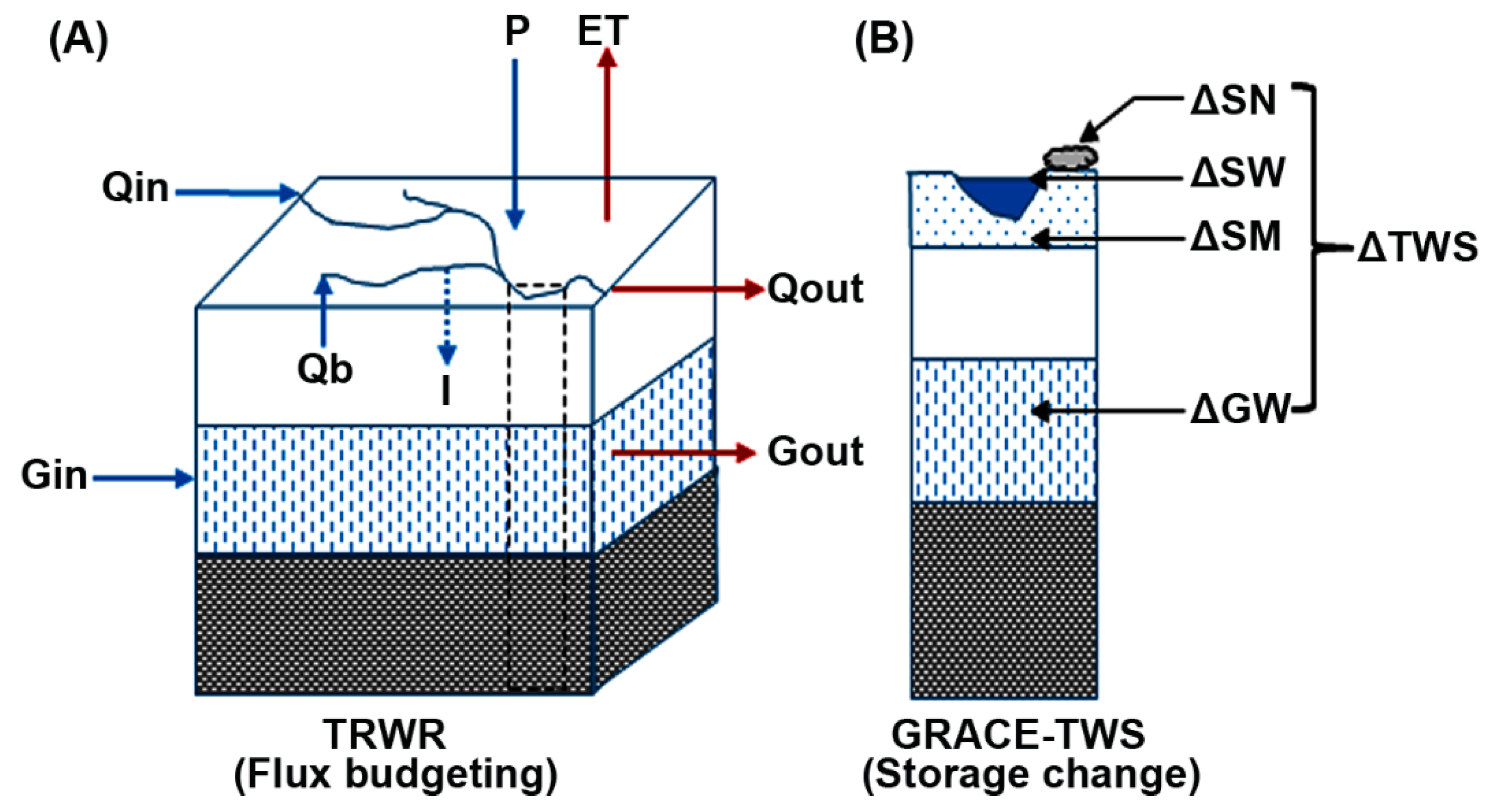
In contrast, the GRACE-based approach integrates all effects of fluxes and anthropogenic factors within the system or study domain and estimates the available water as the net change in storage (Figure 1).
Therefore, to calculate the potential available water storage per-capita (PAWS), first, we estimate the ΔTWS between two consecutive months according to [43].
Because there generally exists a one-month lag between precipitation and TWS [56,57,58], the monthly IWS per-country is determined as the difference between TRMM precipitation estimate of the month(i) and the ΔTWS of the consecutive month(i + 1).
where IWS is expressed in units of mm/month. Then, PAWS is obtained as the average monthly IWS (m/yr.) divided by country population density (population count per unit area).
The PAWS unit is expressed as (m3/yr. per-capita).
We recognize that a degree of difference between IRWR and IWS is inevitable first as a result of errors and uncertainties inherent in the data used to drive each index and second due to the differences in the manner in which available water is conceptualized and calculated. We hypothesize, however, that the two indices will mostly agree when available water per-capita is grouped into different vulnerability classes using the established WSI threshold of Falkenmark (see Table 1). Section 3.2 highlights the differences between the IWS, IRWR, PAWS, and WSI.
2.5. Uncertainty Estimations
The uncertainty associated with each source of data used, that is, TRMM, ΔTWS, lake level estimates, LSM, and the calculated IWS, was assessed according to [52]. Specifically, we applied an additive model approach to decompose the total series into its main constituents as follows:
The standard deviation of the residual, , was treated as a measurement error associated with each component. It is worth noting that the errors calculated in this manner may overestimate the actual error because the residual may contain sub-seasonal scale signals [59].
2.6. TWS Trend Estimation
The TWS trend was estimated using non-parametric Mann-Kendall (MK) trend test [60]. MK method is widely used for trend estimation [61], and the significance of the trend was tested using the Sen’s slope method. The Mann-Kendall statistic for a time series is calculated as,
The MK tests the presence and significance of a trend but not its magnitude. Therefore, we applied Sen’s slope estimator, to determine the magnitude of a trend in each with the statistically significant trend. The test is calculated as,
where and are as previously defined. The slope is measured at points in the time series, , is the median of these values.
We accessed the Sen’s slope algorithm via CARN.R-project, the spatialEco package, for spatial analysis and modeling utilities according to [62].
3. Results and Discussion
3.1. Temporal and Spatial Patterns of ΔTWS
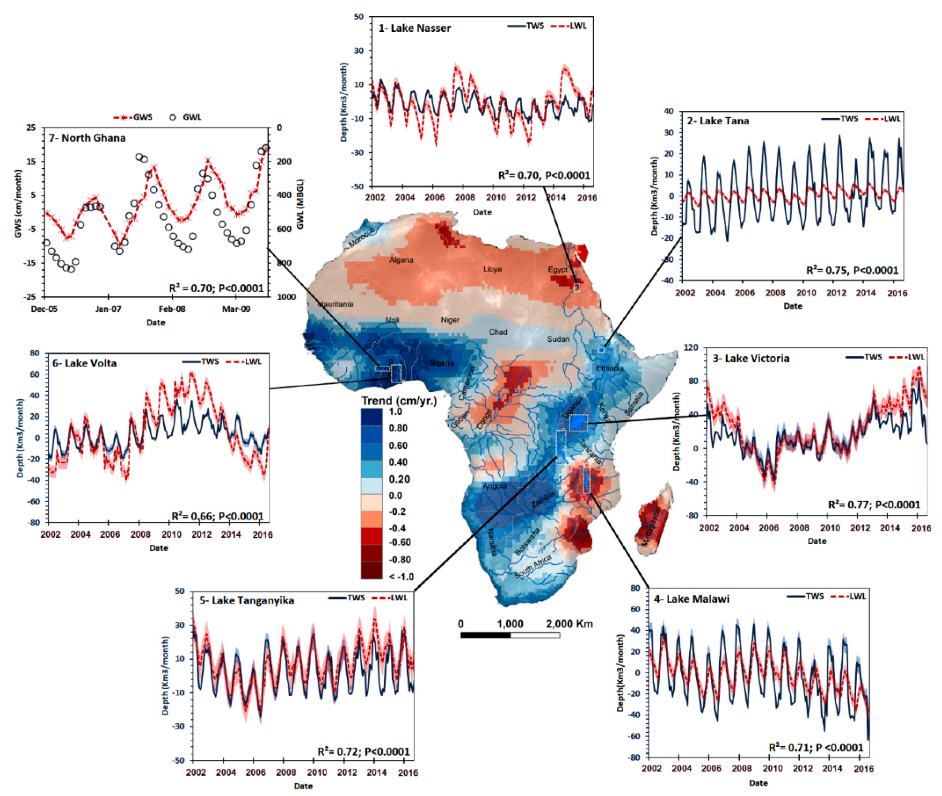
To explore the temporal variation of GRACE-TWS data, Figure 2 compares the monthly TWS series against lake level altimetry observations. The results show the agreement, (R2), between TWS and the lake level observations varying between 0.66 and 0.77, all strongly statistically significant (p < 0.001). This agreement is noteworthy given the small size of the lakes relative to the GRACE footprint. Other important characteristics of the observed lake level time series, such as trends (e.g., Lake Malawi and Lake Tanganyika) and abrupt shifts (e.g., Lake Victoria), are also accurately replicated in TWS observations. On the other hand, the amplitudes are not consistently perfectly matched. This is not surprising, given likely discrepancies between lake surface areas and the GRACE footprint, as well as the fact that GRACE-TWS integrates all the changes in surface and groundwater storage changes, as well as, the variation related to anthropogenic impact [59].
Since GRACE cannot distinguish between anomalies resulting from the surface, soil moisture, or groundwater storage, thus Noah-LSM outputs were used to remove surface and soil moisture storage from GRACE-TWS following Equation (6). The temporal variation of GWS anomalies was compared to in-situ observations to the depths to groundwater levels from twenty groundwater wells in Northern Ghana (Figure 2, plot 7). The two series show good temporal consistency with an R2 value of 0.70 (p < 0.001), similar to the degree of agreement between TWS and lake level measurements.
Spatially, Figure 2 shows the TWS trend of evolution across Africa. Areas of significantly decreasing trend in TWS anomalies are observed in the semiarid and arid regions of North Africa (i.e., Nubian Aquifer and South Tunisia). A large southwest to the northeast oriented region of negative TWS anomalies is extending from the Congo basin to South Sudan. Lake Malawi, Southern Mozambique, and Limpopo river in Southern Africa are displaying negative TWS trend. On the contrary, areas of significant positive TWS trend cover most of Sahel region in West Africa, a large southwest to northeast oriented positive anomalies from Okavango river delta in the southwest, Lake Tanganyika, Lake Victoria, and further northeast to Lake Tana. These observations in TWS trend across Africa were confirmed as well by the temporal patterns from the lake observations. Furthermore, existing studies have concluded similar observations of the TWS trends in Africa (i.e., [38,52,59,63]). However, additional studies are needed to establish the cause(s), as well as associated impacts, of these temporal and spatial patterns of TWS trends across Africa.
3.2. Comparison of IWS, IRWR, PAWS, and WSI
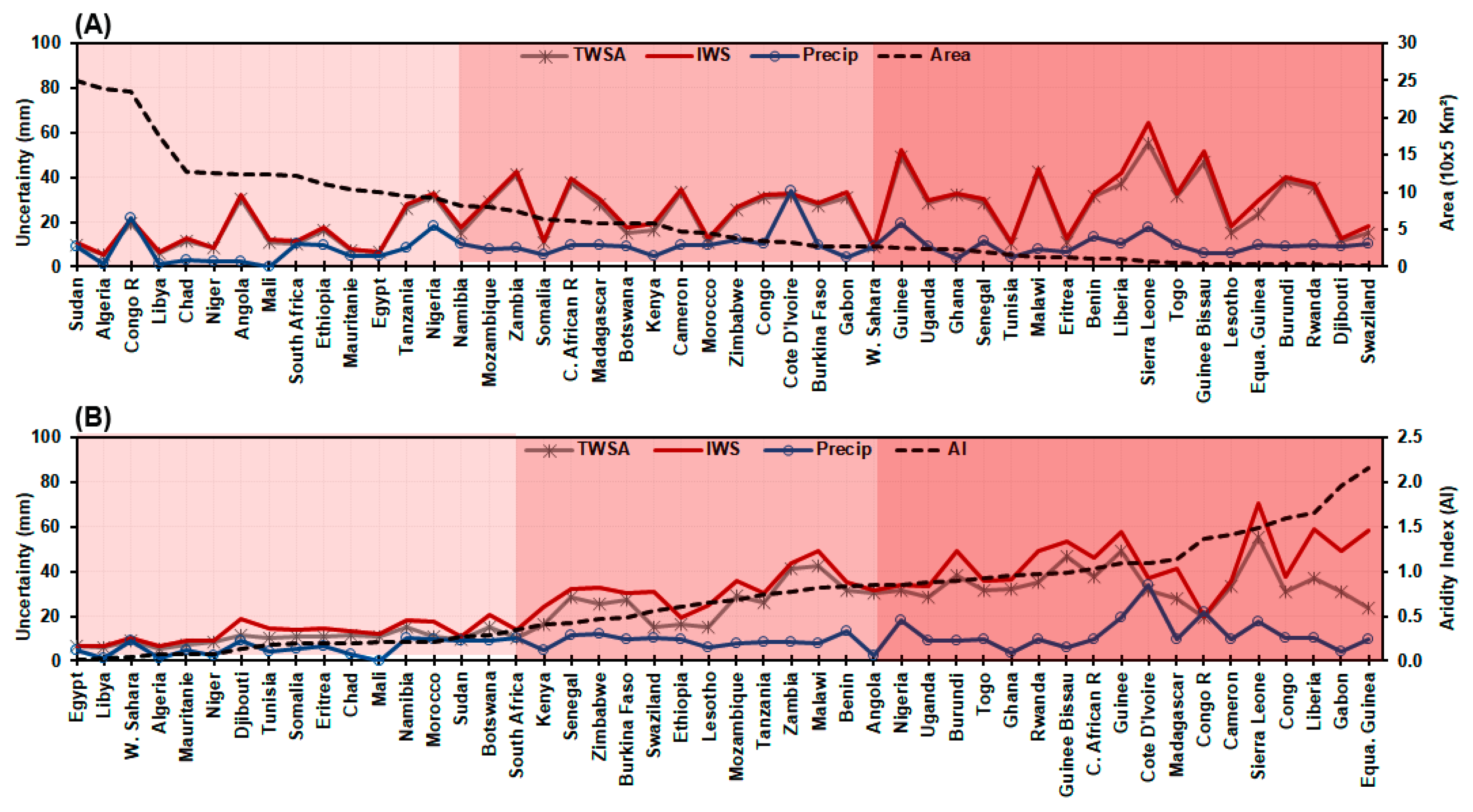
Figure 3 plots the magnitude of uncertainties associated with ΔTWS (TWSA), IWS, and precipitation (Precip). The data have been arranged left to right by decreasing the country’s area (Figure 3A) and increasing the humidity levels according to AI (Figure 3B). The results show that the uncertainty in TWSA and IWS data lies within three averages: ±2 cm, ± 4 cm, and ±6 cm, respectively (see different shades of red in Figure 3). Uncertainty in precipitation is low in all countries, (<± 1 cm), except for Nigeria, Côte d’Ivoire, and Congo. Significantly, the uncertainty in all data sources increases in inverse proportion to country size (R2 = 0.23, p < 0.0001) and direct proportion with the countries’ aridity (R2 = 0.57, p < 0.0001). These findings are consistent with the result of other studies (e.g., [52]), who have also reported larger uncertainties as basin size decreases. Confounding the situation, however, is the fact that the magnitude of uncertainty in the arid zone countries, for example, Egypt, Libya, West Sahara, and Eritrea is also relatively smaller. Since some of the largest countries in Africa by area are also among the most arid, it is unclear how aridity and size affect uncertainty. This is an important area of further research because the results may have implications on the calculations and interpretation of water vulnerability and scarcity using GRACE data.
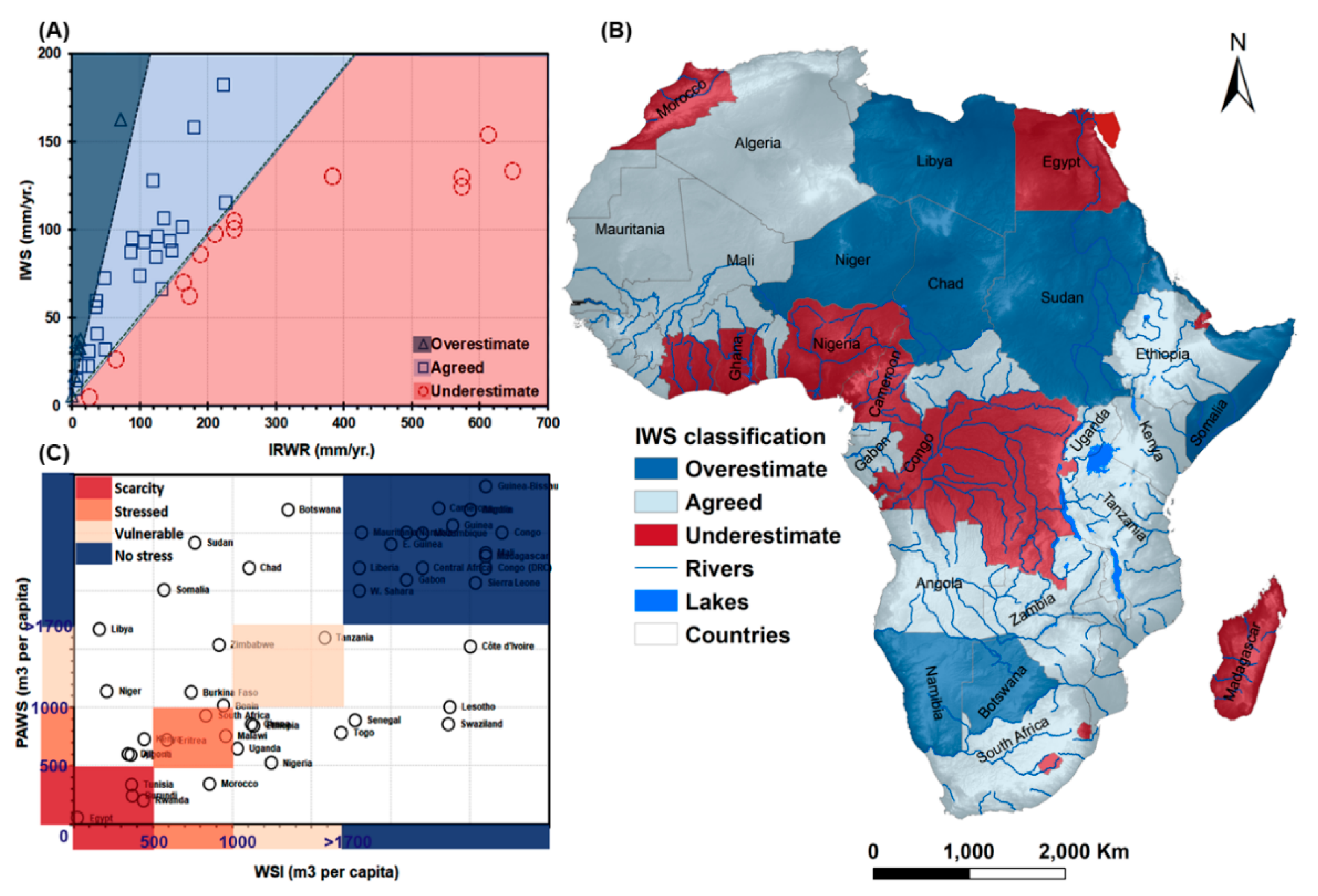
Figure 4A compares the GRACE-estimated IWS to the AQUASTAT-IRWR data by country. The result shows three sets of observations: 1—a good agreement between the calculated IWS and the IRWR in twenty-three countries with (p < 0.0001), 2—overestimation of IWS relative to the IRWR in thirteen countries and finally underestimation between the IWS compared to the IRWR in twelve countries. Spatially, most of the countries, where IWS ‘overestimates’ relative to IRWR, are in arid areas (e.g., Libya, Niger, Kenya, Somali, Namibia) (Figure 4B). We hypothesize that this result likely indicates that IWS includes additional groundwater resources within these countries that are not included in IRWR. Conversely, the countries, where IWS ‘underestimates’, generally have very large populations demanding more water resources (e.g., Egypt, Nigeria, Congo). These observations underscore the contribution of the IWS to update the water resources status of each African country. The countries’ water scarcity classification based on the PAWS indicator shows that 27 countries follow similar pattern compared to the WSI index (Figure 4C).
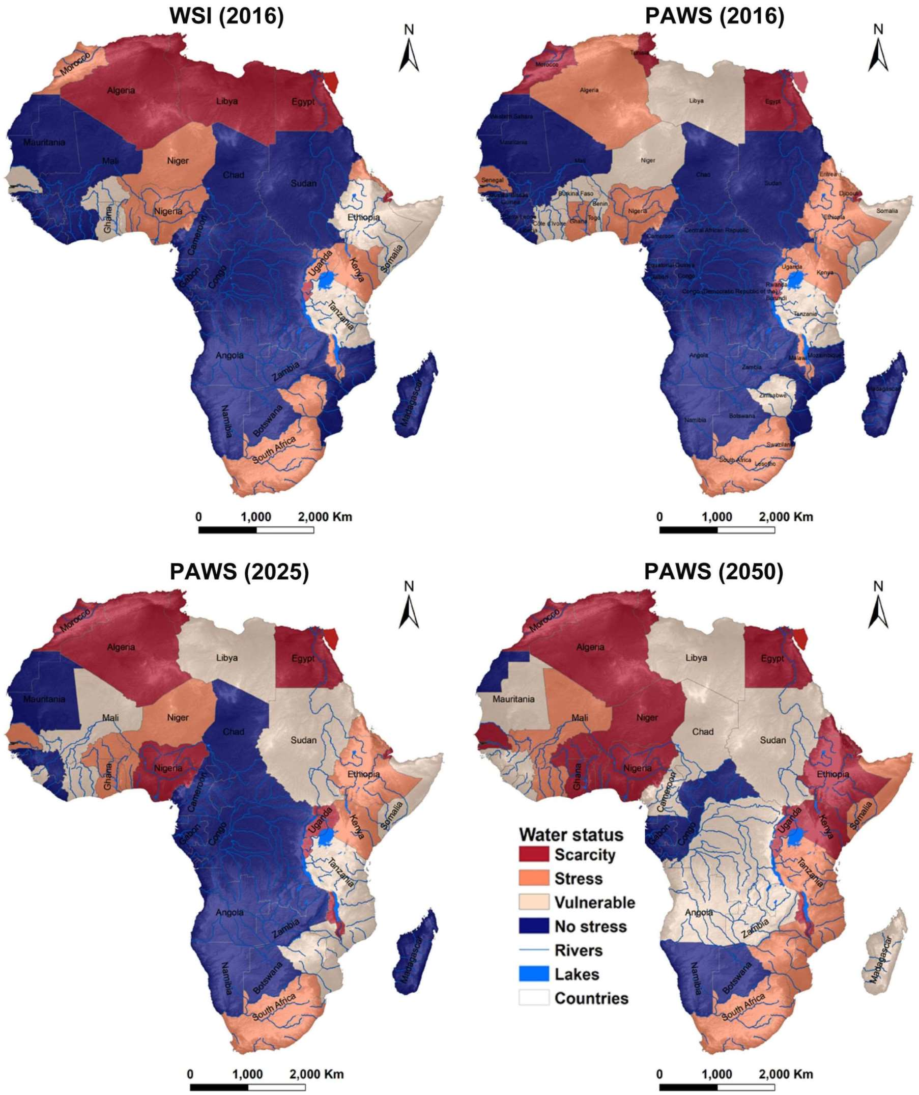
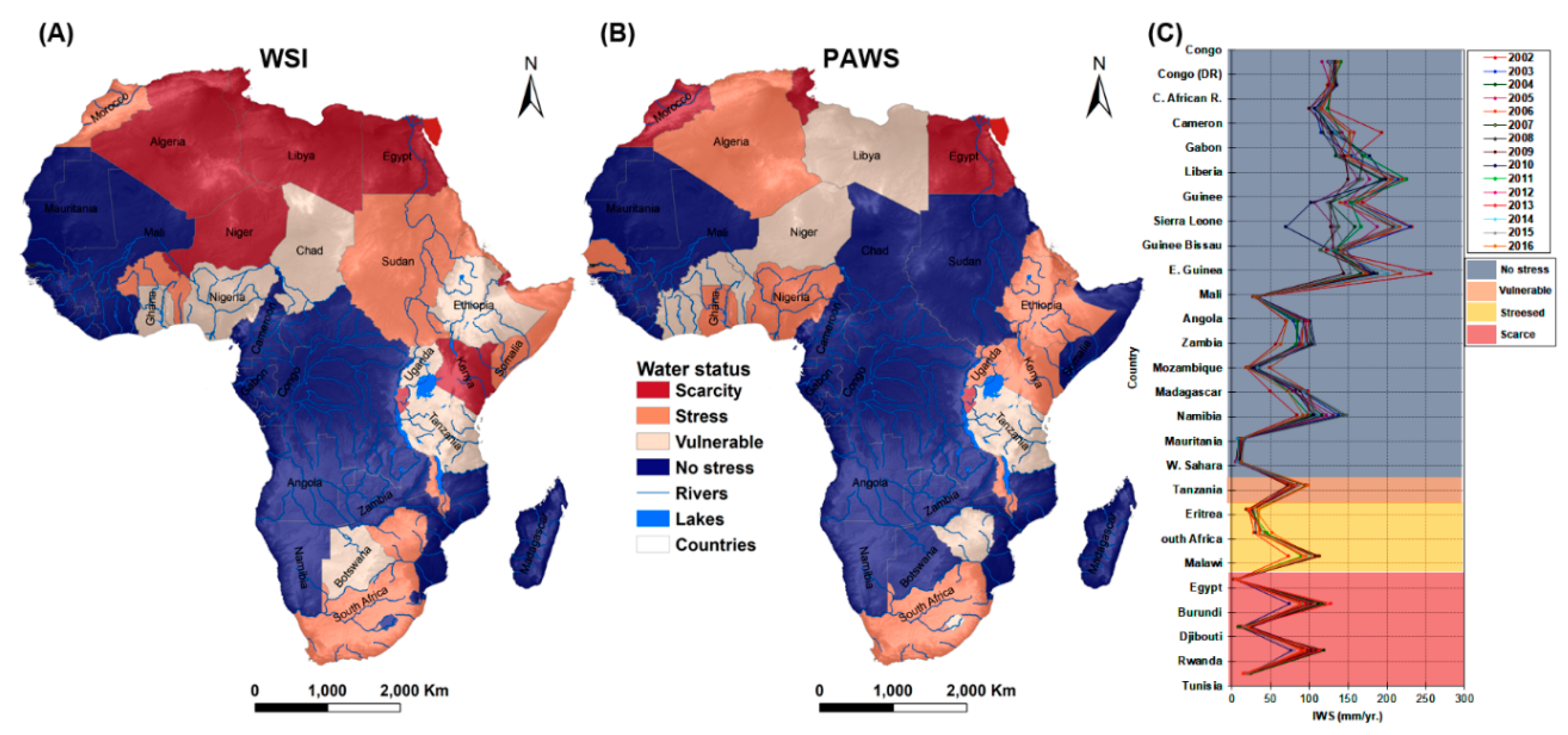
Figure 5 shows the status of water availability in Africa by country based on the WSI (Figure 5A) and PAWS (Figure 5B). Both plots utilize the same water vulnerability thresholds (Table 1). The results show that both the WSI and PAWS classify twenty-six countries (54%) into the same water vulnerability class (Figure 5C). Much of this agreement is driven by the countries classified as experiencing ‘no stress’, out of which eighteen (69%) are classified similarly. Of the remaining, one country (Tanzania) is classified by both PWAS and WSI as “vulnerable”, three countries are classified as stressed (Eretria, Malawi, and South Africa), and four are classified as scarce in both indices (Egypt, Tunisia, Rwanda, and Burundi). In twenty-two countries (45%), however, the two indices lead to a different water vulnerability status. For instance, the PAWS index leveled up twelve countries in their water vulnerability status, while ten countries were leveled down compared to WSI indicator (see Figure 5).
The above patterns reveal important differences between PAWS and WSI. For example, considering both the scarcity and stressed categories, the agreement in the countries classified similarly is 54%, implying that the methods agree more than they disagree. Based on the water vulnerability levels, the PAWS index revealed that about 14% of the African population, ~160 million people, currently live under a water scarcity status. Meanwhile, according to WSI, about 20% of the African population, ~250 million people, currently live under water scarcity conditions. Research is needed to clarify areas of disagreement in water vulnerability status classification between the proposed PAWS and existing methods based on conventional data. Meanwhile, the differences are mainly attributed to the dynamic changes recorded by GRACE-based IWS between 2002 and 2016 (Figure 5C). Moreover, the apparent high level of agreement in the countries classified as ‘no-stress’ may simply be due to the fact that this category is large and unbounded on the upper end, allowing many more countries to be grouped together. As noted previously, these differences are not surprising. The PAWS estimate accounts for all forms of water, including soil moisture and groundwater in deep aquifers, while WSI relies overwhelmingly on the portion of water influx within the system. The WSI likely underestimates, especially, the groundwater component due to poor data availability and quality. Furthermore, the runoff and flow measurements are highly susceptible to measurement and calibration errors. In contrast, not all of the water available in storage as measured by PAWS is extractable for technical and economic reasons. Therefore, the method likely overestimates real or useable available water. Further research is also required to reconcile these inconsistencies to facilitate decision making and planning regarding the water vulnerability status of African countries.
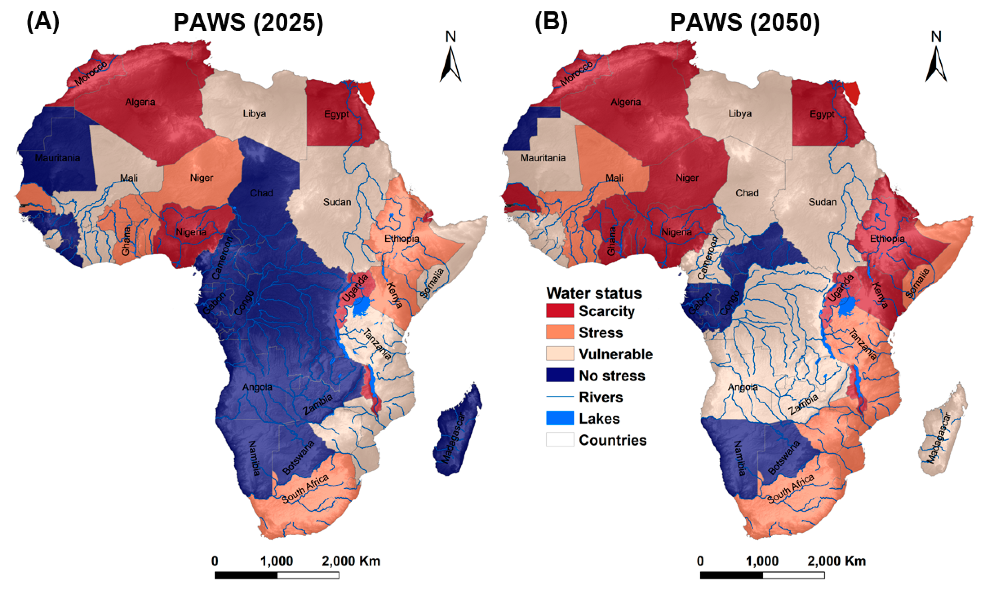
The PAWS index has utilized to develop the first-order estimates of possible water scarcity levels due to projected climate change and population growth in Africa. A 10% decrease in future water resources, which is within the range of several climate projections for some countries [64], is developed for future population growth of years 2025 and 2050. Figure 6 shows that total water resources availability in the year 2025 leads to ~100% increase in the number of countries experiencing water scarcity, from five to ten countries. This implies that ~37% or ~600 million people of Africa’s population would be affected. Meanwhile, the number of countries under scarcity condition increased ~280% for the year 2050, from five to nineteen countries. This means that ~57% of Africa’s population or about 1.4-billion people will deal with the extreme water crisis. Within the water scarcity continuum, for 2025, the number of countries experiencing water stress decreases from twelve to nine, while, thirteen are classified as vulnerable. Interestingly, the 2025 projections reveal that seventeen countries which are currently classified as “no stress” still lie under the same water scarcity category. The projections for the year 2050 show that the total number of countries experiencing “no stress” status is declined significantly from seventeen to seven countries, meaning that ~85% of Africa will face a dangerous water scarcity situation by 2050.
These future scenarios present a sobering picture of the precarious situation of water availability in Africa given rapid population growth. Fortunately, it is highly unlikely that the entire continent will experience a 10% decrease in water resources availability everywhere. Even so, for some countries, one or more of these scenarios are within the range of past experience. For example, the peak of the Sahel droughts of 1970 to 1985, precipitation decreased by 30% [65,66], suggesting that such a magnitude of change is possible again at some point in the future. Moreover, a number of climate change projection scenarios suggest a decrease in precipitation over Northern Africa and the Western parts of Africa [67], while the Eastern and Southern Africa are highly likely to experience increase precipitation by the end of the 21st century [68,69].
4. Conclusions
Availability of freshwater resources is critical for assuring human wellbeing, socio-economic development, and food security. This pivotal and ubiquitous role leads to great interest in determining as accurately as possible the status of freshwater resources availability as a basis for developing policies for planning and water resources utilization or allocation. Currently, the most widely used method of obtaining this information relies on the measurements of the fluxes of water entering and exiting a country. Unfortunately, the requisite data tends to be unavailable, discontinuous over space and time, inaccessible for reasons of conflict or political decisions, and frequently collected by different agencies using different references periods and standards.
In this paper, we demonstrated the use of GRACE anomalies and TRMM precipitation estimates for calculating available renewable water resources for Africa. The proposed approach overcomes many of the limitations identified above. The data are accessible, continuous over space and time, and collected based on a consistent methodology and reference period. Even so, the method is not without limitations. Critically, it estimates potential available fresh water only in a hydrologic or physical sense. That is, it does not address the political and power relations that make water actually available or accessible. Additionally, the method as presented deals with water scarcity at the country level, an often-cited criticism of many existing methods. While the methodology is perfectly capable of being applied at finer temporal, political, and geographic units, we elected to focus on the country level because of the availability of the AQUASTAT-IRWR data against which we have compared our results. The major findings can be summarized as follows:
- Estimates of TWS derived from GRACE appear to be affected by country size and aridity. The magnitude of uncertainty associated with input data increases as the country size decreases. However, the relationship is complicated by the fact that many of Africa’s largest countries inhabit the most arid zones. Either factor has a physical basis. Confidence in GRACE estimates decreases as the study domain shrinks to below 200,000 km2, generally accepted as the GRACE footprint. Similarly, the small range of variability in available water typical in arid regions leads to smaller uncertainty in estimated TWS. Further research is needed to establish the relative effects of scale and aridity on GRACE anomalies.
- With the above caveat in mind, the PAWS approach classifies 26 out of 48 countries in the same water vulnerable category as AQUASTAT-IRWR. Of the remaining countries, a strong majority was classified in the adjoining or bordering category, suggesting that the hard thresholds contribute to some of the differences in classification. On the other hand, much of the agreement between the two methods is driven by the large no stress category, which acts as a sort of catchall group. This suggests, perhaps not unexpectedly, that the differences between the two methods are accentuated when using small ranges for categorization. Clearly, however, there are fundamental differences between WSI and PAWS, which reflect how available water is conceptualized and calculated.
- Compared to the IRWR, PAWS results in a more moderate assessment of water resources scarcity in the arid areas. This is not surprising, given the spatial continuity of the PAWS estimates compared to the country averaged-IRWR. Additionally, we suspect that PAWS index integrates a larger proportion of groundwater, accounting for the difference.
- The PAWS can be used to rapidly develop first estimates or scenarios of possible water scarcity due to climate change and population growth. A 10% decrease in future water resources, which is within the range of several climate projections for some countries, may entail a significant increase in the number of additional countries facing water scarcity. Preliminary analysis suggests that it is possible to partition GRACE signals to yield proxy estimates of groundwater measurements, although more data are needed in different climatic zones in order to develop robust calibration. Additional research is needed to expand and validate the promise shown by these preliminary estimates, including, for example, the ability to partition GRACE signals to derive proxies for groundwater level dynamics and to investigate water scarcity at finer spatial and temporal time scales.
Author Contributions
Conceptualization, E.H. and A.T.; methodology, E.H. and A.T.; Validation, E.H.; formal analysis, E.H.; resources, Y.H. and B.M.III; writing—original draft preparation, E.H. and A.T.; writing—review and editing, E.H. and A.T.; supervision, A.T. and Y.H.; funding acquisition, B.M.III; A.T. and Y.H.
Funding
This research was funded by the National Mesonet Project (NMP) (Grant No. 105436100–Moore).
Acknowledgments
The authors thank the College of Atmospheric and Geographic Sciences (A&GS) at the University of Oklahoma (OU) and the Provost’s office at the State University of New York (SUNY) at Binghamton for providing research funds to this study. Thanks also go to the Advanced Radar Research Center and the Hydrometeorology and Remote Sensing Laboratory (HyDROS) at OU for providing the research facilities, workspace, and equipment to accomplish this research. The authors are grateful to David N Wiese from NASA JPL and Mohamed Ahmed from the University of Texas A&M University-Corpus Christi for the discussion that helped in the manuscript preparation. We are also thankful to the three anonymous reviewers for their valuable comments and suggestions, which improved the overall quality of our paper. We also wish to thank the providers of some important remote sensing and reanalysis datasets used in this research: The Center for Space Research (CSR) at the University of Texas, Austin, NASA Goddard Earth Science Data and Information Service Centers, Climate Research Unit, the British Geological Survey, the AQUASTAT FAO’s global water information system, and the World Bank database center.
Conflicts of Interest
The authors also would declare that there is no conflict of interest.
References
- Rijsberman, F.R. Water scarcity: Fact or fiction? Agric. Water Manag. 2006, 80, 5–22. [Google Scholar] [CrossRef] [Green Version]
- Mekonnen, M.M.; Hoekstra, A.Y. Four billion people facing severe water scarcity. Sci. Adv. 2016, 2, 1–6. [Google Scholar] [CrossRef] [PubMed]
- Liu, J.; Yang, H.; Gosling, S.N.; Kummu, M.; Flörke, M.; Pfister, S.; Hanasaki, N.; Wada, Y.; Zhang, X.; Zheng, C.; et al. Water scarcity assessments in the past, present and future. Earth’s Future 2017, 5, 545–559. [Google Scholar] [CrossRef] [PubMed] [Green Version]
- FAO. Coping with Water Scarcity an Action Framework for Agriculture and Food Security; FAO: Rome, Italy, 2012; p. 78. [Google Scholar]
- Sambu, D. Water Reforms in Kenya: A Historical Challenge to Ensure Universal Water Access and Meet the Millennium Development Goals. Ph.D. Thesis, The University of Oklahoma, Ann Arbor, MI, USA, 2011. [Google Scholar]
- Falkenmark, M.; Widstrand, C. Population and Water Resources: A Delicate Balance. Popul. Bull. 1992, 47, 1–36. [Google Scholar]
- Savenije, H.H.G. Water Scarcity Indicators; the Deception of the Numbers. Phys. Chem. Earfh (B) 2000, 25, 199–204. [Google Scholar] [CrossRef]
- White, C. Understanding Water Scarcity: Definitions and Measurements; Global Water Forum: In Water Security. 2012. Available online: http://www.globalwaterforum.org/2012/05/07/understanding-water-scarcity-definitions-and-measurements/ (accessed on 25 May 2016).
- Molle, F.; Mollinga, P. Water poverty indicators: Conceptual problems and policy issues. Water Policy 2003, 5, 529–544. [Google Scholar] [CrossRef]
- Falkenmark, M. The Massive Water Scarcity Now Threatening Africa: Why Isn’t It Being Addressed? Ambio 1989, 18, 112–118. [Google Scholar]
- Shiklomanov, I.A. World fresh water resources. In Water in Crisis: A Guide to the World’s Fresh Water Resources; Gleick, P.H., Ed.; Pacific Institute for Studies In development, Environment, and Security Stockholm Environment Institute: New York, NY, USA; Oxford, UK, 1993. [Google Scholar]
- Gleick, P.H. Basic Water Requirements for Human Activities: Meeting Basic Needs. Water Int. 1996, 21, 83–92. [Google Scholar]
- Yang, H.; Reichert, P.; Abbaspour, K.C.; Zehnder, A.J.B. A Water Resources Threshold and Its Implications for Food Security. Environ. Sci. Technol. 2003, 37, 3048–3054. [Google Scholar] [CrossRef] [PubMed] [Green Version]
- Chaves, H.M.L.; Alipaz, S. An Integrated Indicator Based on Basin Hydrology, Environment, Life, and Policy: The Watershed Sustainability Index. Water Resour. Manag. 2006, 21, 883–895. [Google Scholar] [CrossRef]
- Seckler, D.; Amarasinghe, U.; Molden, D.J.; Silva, R.D.; Barker, R. World Water Demand and Supply, 1990 to 2025: Scenarios and Issues; IWMI: Colombo, Sri Lanka, 1998. [Google Scholar]
- Rockström, J.; Falkenmark, M.; Karlberg, L.; Hoff, H.; Rost, S.; Gerten, D. Future water availability for global food production: The potential of green water for increasing resilience to global change. Water Resour. Res. 2009, 45. [Google Scholar] [CrossRef] [Green Version]
- Hoekstra, A.Y.; Chapagain, A.K.; Aldaya, M.M.; Mekonnen, M.M. The Water Footprint Assessment Manual: Setting the Global Standard; Earthscan: London, DC, USA, 2011. [Google Scholar]
- Ohlsson, L. Water Conflicts and Social Resource Scarcity. Phys. Chem. Earth (B) 2000, 25, 213–220. [Google Scholar] [CrossRef]
- Alcamo, J.; Henrichs, T. Critical regions: A model-based estimation of world water resources sensitive to global changes. Aquat. Sci. 2002, 64, 352–362. [Google Scholar] [CrossRef]
- Vorosmarty, C.J.; Douglas, E.M.; Green, P.A.; Revenga, C. Geospatial Indicators of Emerging Water Stress: An Application to Africa. Ambio (R. Sweedish Acad. Sci.) 2005, 34, 230–236. [Google Scholar] [CrossRef]
- Lawrence, P.; Meigh, J.; Sullivan, C. The Water Poverty Index: An International Comparison; Department of Economics, Keele University: Keele, UK, 2002. [Google Scholar]
- McNulty, S.; Sun, G.; Myers, J.M.; Cohen, E.; Caldwell, P. Robbing Peter to Pay Paul: Tradeoffs Between Ecosystem Carbon Sequestration and Water Yield. In Proceedings of the Environmental Water Resources Institute Meeting, Madison, WI, USA, 23–27 August 2010. [Google Scholar]
- Gerten, D.; Heinke, J.; Hoff, H.; Biemans, H.; Fader, M.; Waha, K. Global Water Availability and Requirements for Future Food Production. J. Hydrometeorol. 2011, 12, 885–899. [Google Scholar] [CrossRef]
- AQUASTAT. Freshwater Availability—Precipitation and Internal Renewable Water Resources (IRWR); Food and Agriculture Orgnization (FAO) of the United Nation (UN): Rome, Italy, 2014. [Google Scholar]
- Bertsch, M. Exploring Alternative Futures of the World Water System. Building a Second Generation of World Water Scenarios Driving Force: Water Resources and Ecosystems; United Nations World Water Assessment Programme (UN WWAP): Perugia, Italy, 2010. [Google Scholar]
- Naik, P.K. Water crisis in Africa: Myth or reality? Int. J. Water Resour. Dev. 2017, 33, 326–339. [Google Scholar] [CrossRef]
- Save, H.; Bettadpur, S.; Tapley, B.D. High-resolution CSR GRACE RL05 mascons. J. Geophys. Res. Solid Earth 2016, 121, 7547–7569. [Google Scholar] [CrossRef]
- Huffman, G.; Bolvin, D.; Braithwaite, D.; Hsu, K.; Joyce, R.; Xie, P. Integrated Multi-satellitE Retrievals for GPM (IMERG), version 4.4. NASA’s Precipitation Processing Center. Available online: ftp://arthurhou.pps.eosdis.nasa.gov/gpmdata/ (accessed on 15 March 2018).
- Harris, I.; Jones, P.D.; Osborn, T.J.; Lister, D.H. Updated high-resolution grids of monthly climatic observations—The CRU TS3.10 Dataset. Int. J. Climatol. 2014, 34, 623–642. [Google Scholar] [CrossRef]
- Rodell, M.; Houser, P.R.; Jambor, U.; Gottschalck, J.; Mitchell, K.; Meng, C.J.; Arsenault, K.; Cosgrove, B.; Radakovich, J.; Bosilovich, M.; et al. The Global Land Data Assimilation System. Bull. Am. Meteorol. Soc. 2004, 85, 381–394. [Google Scholar] [CrossRef] [Green Version]
- Cretaux, J.F.; Jelinski, W.; Calmant, S.; Kouraev, A.; Vuglinski, V.; Berge-Nguyen, M.; Gennero, M.C.; Nino, F.; Del Rio, R.A.; Cazenave, A.; et al. SOLS: A lake database to monitor in the Near Real Time water level and storage variations from remote sensing data. Adv. Space Res. 2011, 47, 1497–1507. [Google Scholar] [CrossRef]
- Gokmen, M.; Vekerdy, Z.; Lubczynski, M.W.; Timmermans, J.; Batelaan, O.; Verhoef, W. Assessing Groundwater Storage Changes Using Remote Sensing–Based Evapotranspiration and Precipitation at a Large Semiarid Basin Scale. J. Hydrometeorol. 2013, 14, 1733–1753. [Google Scholar] [CrossRef]
- Swenson, S.; Famiglietti, J.; Basara, J.; Wahr, J. Estimating profile soil moisture and groundwater variations using GRACE and Oklahoma Mesonet soil moisture data. Water Resour. Res. 2008, 44, 1–12. [Google Scholar] [CrossRef]
- Landerer, F.W.; Swenson, S.C. Accuracy of scaled GRACE terrestrial water storage estimates. Water Resour. Res. 2012, 48, 1–11. [Google Scholar] [CrossRef]
- Hasan, E.; Tarhule, A.; Hong, Y.; Moore, B., III. Potential Water Availability Index (PWAI): A New Water Vulnerability Index for Africa Based on GRACE Data. In Proceedings of the American Geophysical Union, Fall Meeting, San Francisco, CA, USA, 12–16 December 2016. [Google Scholar]
- Hassan, A.A.; Jin, S. Lake level change and total water discharge in East Africa Rift Valley from satellite-based observations. Glob. Planet. Chang. 2014, 117, 79–90. [Google Scholar] [CrossRef]
- Hasan, E.; Dokou, Z.; Kirstetter, P.-E.; Tarhule, A.; Anagnostou, E.N.; Bagtzoglou, A.C.; Hong, Y. Assessing Lake Level Variability and Water Availability in Lake Tana, Ethiopia using a Groundwater Flow Model and GRACE Satellite Data. In Proceedings of the AGU Fall Meeting, New Orleans, LA, USA, 11–15 December 2017. [Google Scholar]
- Ahmed, M.; Sultan, M.; Wahr, J.; Yan, E. The use of GRACE data to monitor natural and anthropogenic induced variations in water availability across Africa. Earth-Sci. Rev. 2014, 136, 289–300. [Google Scholar] [CrossRef]
- Frappart, F.; Ramillien, G. Monitoring Groundwater Storage Changes Using the Gravity Recovery and Climate Experiment (GRACE) Satellite Mission: A Review. Remote Sens. 2018, 10, 829. [Google Scholar] [CrossRef]
- Rodell, M.; Chen, J.; Kato, H.; Famiglietti, J.S.; Nigro, J.; Wilson, C.R. Estimating groundwater storage changes in the Mississippi River basin (USA) using GRACE. Hydrogeol. J. 2006, 15, 159–166. [Google Scholar] [CrossRef] [Green Version]
- Syed, T.H.; Famiglietti, J.S.; Chambers, D.P. GRACE-Based Estimates of Terrestrial Freshwater Discharge from Basin to Continental Scales. J. Hydrometeorol. 2009, 10, 22–40. [Google Scholar] [CrossRef]
- Swenson, S.; Wahr, J. Estimating Large-Scale Precipitation Minus Evapotranspiration from GRACE Satellite Gravity Measurements. J. Hydrometeorol. 2006, 7, 252–270. [Google Scholar] [CrossRef]
- Rodell, M.; Famiglietti, J.S.; Chen, J.; Seneviratne, S.I.; Holl, P.V.; Wilson, C.R. Basin scale estimates of evapotranspiration using GRACE and other observations. Geophys. Res. Lett. 2004, 31, 1–4. [Google Scholar] [CrossRef]
- Wan, Z.; Zhang, K.; Xue, X.; Hong, Z.; Hong, Y.; Gourley, J.J. Water balance-based actual evapotranspiration reconstruction from ground and satellite observations over the conterminous United States. Water Resour. Res. 2015, 51, 6485–6499. [Google Scholar] [CrossRef] [Green Version]
- Ramillien, G.; Frappart, F.; Güntner, A.; Ngo-Duc, T.; Cazenave, A.; Laval, K. Time variations of the regional evapotranspiration rate from Gravity Recovery and Climate Experiment (GRACE) satellite gravimetry. Water Resour. Res. 2006, 42. [Google Scholar] [CrossRef] [Green Version]
- Longuevergne, L.; Scanlon, B.R.; Wilson, C.R. GRACE Hydrological estimates for small basins: Evaluating processing approaches on the High Plains Aquifer, USA. Water Resour. Res. 2010, 46. [Google Scholar] [CrossRef] [Green Version]
- Reager, J.T.; Famiglietti, J.S. Characteristic mega-basin water storage behavior using GRACE. Water Resour. Res. 2013, 49, 3314–3329. [Google Scholar] [CrossRef] [PubMed] [Green Version]
- Tapley, B.D.; Bettadpur, S.; Ries, J.C.; Thompson, P.F.; Watkins, M.M. GRACE Measurements of Mass Variability in the Earth System. Science 2004, 305, 503. [Google Scholar] [CrossRef] [PubMed]
- Luthcke, S.B.; Rowlands, D.D.; Sabaka, T.J.; Loomis, B.D.; Horwath, M.; Arendt, A.A. Gravimetry Measurements from Space; Wiley Blackwell: Oxford, UK, 2015; Volume 10. [Google Scholar]
- Rowlands, D.D.; Luthcke, S.B.; Klosko, S.M.; Lemoine, F.G.R.; Chinn, D.S.; McCarthy, J.J.; Cox, C.M.; Anderson, O.B. Resolving mass flux at high spatial and temporal resolution using GRACE intersatellite measurements. Geophys. Res. Lett. 2005, 32. [Google Scholar] [CrossRef] [Green Version]
- Watkins, M.M.; Wiese, D.N.; Yuan, D.-N.; Boening, C.; Landerer, F.W. Improved methods for observing Earth’s time variable mass distribution with GRACE using spherical cap mascons. J. Geophys. Res. Solid Earth 2015, 120, 2648–2671. [Google Scholar] [CrossRef]
- Scanlon, B.R.; Zhang, Z.; Save, H.; Wiese, D.N.; Landerer, F.W.; Long, D.; Longuevergne, L.; Chen, J. Global evaluation of new GRACE mascon products for hydrologic applications. Water Resour. Res. 2016, 52, 9412–9429. [Google Scholar] [CrossRef] [Green Version]
- Normandin, C.; Frappart, F.; Diepkilé, A.T.; Marieu, V.; Mougin, E.; Blarel, F.; Lubac, B.; Braquet, N.; Ba, A. Evolution of the Performances of Radar Altimetry Missions from ERS-2 to Sentinel-3A over the Inner Niger Delta. Remote Sens. 2018, 10, 833. [Google Scholar] [CrossRef]
- Middleton, N.; Thomas, D.S.G.; United Nations Environment Programme. World Atlas of Desertification; UNEP: London, UK, 1992. [Google Scholar]
- Weiskel, P.K.; Vogel, R.M.; Steeves, P.A.; Zarriello, P.J.; DeSimone, L.A.; Ries, K.G. Water use regimes: Characterizing direct human interaction with hydrologic systems. Water Resour. Res. 2007, 43. [Google Scholar] [CrossRef] [Green Version]
- Humphrey, V.; Gudmundsson, L.; Seneviratne, S.I. Assessing Global Water Storage Variability from GRACE: Trends, Seasonal Cycle, Subseasonal Anomalies and Extremes. Surv. Geophys. 2016, 37, 357–395. [Google Scholar] [CrossRef] [PubMed] [Green Version]
- Ahmed, M.; Sultan, M.; Wahr, J.; Yan, E.; Milewski, A.; Sauck, W.; Becker, R.; Welton, B. Integration of GRACE (Gravity Recovery and Climate Experiment) data with traditional data sets for a better understanding of the time-dependent water partitioning in African watersheds. Geology 2011, 39, 479–482. [Google Scholar] [CrossRef]
- Papa, F.; Güntner, A.; Frappart, F.; Prigent, C.; Rossow, W.B. Variations of surface water extent and water storage in large river basins: A comparison of different global data sources. Geophys. Res. Lett. 2008, 35. [Google Scholar] [CrossRef] [Green Version]
- Scanlon, B.R.; Zhang, Z.; Save, H.; Sun, A.Y.; Muller Schmied, H.; van Beek, L.P.H.; Wiese, D.N.; Wada, Y.; Long, D.; Reedy, R.C.; et al. Global models underestimate large decadal declining and rising water storage trends relative to GRACE satellite data. Proc. Natl. Acad. Sci. USA 2018, 115, E1080–E1089. [Google Scholar] [CrossRef] [Green Version]
- Kendall, M.G. Rank Correlation Methods; Griffin: London, UK, 1975. [Google Scholar]
- Gocic, M.; Trajkovic, S. Analysis of changes in meteorological variables using Mann-Kendall and Sen’s slope estimator statistical tests in Serbia. Glob. Planet. Chang. 2013, 100, 172–182. [Google Scholar] [CrossRef]
- Evans, J.S.; Ram, K. spatialEco: Spatial Analysis and Modelling Utilities. Available online: https://cran.r-project.org/package=spatialEco (accessed on 21 December 2018).
- Werth, S.; White, D.; Bliss, D.W. GRACE Detected Rise of Groundwater in the Sahelian Niger River Basin. J. Geophys. Res. Solid Earth 2017, 122, 10459–10477. [Google Scholar] [CrossRef]
- Hasan, E.; Tarhule, A.; Kirstetter, P.-E.; Clark, R.; Hong, Y. Runoff sensitivity to climate change in the Nile River Basin. J. Hydrol. 2018, 561, 312–321. [Google Scholar] [CrossRef]
- Nicholson, S.E. Climatic and environmental change in Africa during the last two centuries. Clim. Res. 2001, 17, 123–144. [Google Scholar] [CrossRef] [Green Version]
- Dai, A.; Lamb, P.J.; Trenberth, K.E.; Hulme, M.; Jones, P.D.; Xie, P. The recent Sahel drought is real. Int. J. Climatol. 2004, 24, 1323–1331. [Google Scholar] [CrossRef] [Green Version]
- Dunning, C.M.; Black, E.; Allan, R.P. Later Wet Seasons with More Intense Rainfall over Africa under Future Climate Change. J. Clim. 2018, 31, 9719–9738. [Google Scholar] [CrossRef]
- Shongwe, M.E.; van Oldenborgh, G.J.; van den Hurk, B.; van Aalst, M. Projected Changes in Mean and Extreme Precipitation in Africa under Global Warming. Part II: East Africa. J. Clim. 2011, 24, 3718–3733. [Google Scholar] [CrossRef]
- Bucchignani, E.; Mercogliano, P.; Panitz, H.-J.; Montesarchio, M. Climate change projections for the Middle East–North Africa domain with COSMO-CLM at different spatial resolutions. Adv. Clim. Chang. Res. 2018, 9, 66–80. [Google Scholar] [CrossRef]
Figure 1.
A conceptual framework to estimate the net water storage using flux budgeting (A) as the difference between the input-output of the water in the system and Gravity Recovery and Climate Experiment (GRACE)-based changes in water storage (B). TRWR: Total Renewable Water Resources; Qin: inflow; Qb: baseflow; Qout: outflow; I: infiltration; Gin: groundwater-in; Gout: groundwater-out; TWS: Total Water Storage; SN: Snowpack; SW: Surface Water; GW: Ground Water; SM: Soil Moisture.

Figure 2.
Total Water Storage (TWS) trend across Africa between 2002 and 2016 derived using the Center for Space Research (CSR)-M data. The trend map shows a varying TWS across Africa with a remarkable decline in North Africa, Congo basin in the west, Lake Malawi, Limpopo river basin, and Madagascar in South Africa. There is a positive increase in TWS in the Sahel region in the west, Okavango river basin in the south, Lake Victoria, and Lake Tana. The TWS signals from CSR-M were compared with lake water level (LWL) observations across six major lakes. Noteworthy, the majority of the lakes have aerial coverage less than the original Gravity Recovery and Climate Experiment (GRACE) satellite footprint; however, there is good consistency between GRACE signals and lake level anomalies (p-value < 0.0001). The uncertainty bounds are computed for the TWS and LWL as introduced in Section 2.5. Additionally, groundwater storage estimates from GRACE, based on Equation (6), were compared to groundwater levels (meter below ground level-MBGL) that were averaged from 20 groundwater wells in North Ghana. The in-situ groundwater observation covers the period from December 2005 to December 2009. The GRACE-based groundwater observations show good agreement with the in-situ data (p-value < 0.0001).

Figure 3.
Uncertainty estimates of all variables calculated according to Equation (10) relative to countries area (A) and the aridity index (B). The aridity is calculated as the ratio of P/PET and classified following [54]. Areas of red shades indicate the average uncertainties for Total Water Storage Anomaly (TWSA) and Internal Water Storage (IWS) data.

Figure 4.
Estimated countries’ Internal Water Storage (IWS) versus the AQUASTAT- Internal Renewable Water Resources (IRWR) (A), this plot indicates the three main classes of the estimation (agreed, overestimate, and underestimate), the spatial distribution of these classes is shown in the map (B). Based on the calculated IWS, the Potential Available Water Storage (PAWS) will follow the same pattern when compared to Water Scarcity Index (WSI) indicator (C).

Figure 5.
Water Stress Index based on the current AQUASTAT water storage data (A), and the new proposed Potential Available Water Storage (PAWS) from Gravity Recovery and Climate Experiment (GRACE) data (B) using the average Internal Water Storage (IWS) from 2002 to 2016. The plot (C) shows the changes in the IWS for 26 countries between 2002 and 2016 that are agreed on the water status level, (“no stress” 18 countries, “vulnerable” one country, “Stressed” three countries, and “Scarce” four countries).

Figure 6.
Future water status based on 10% decrease in the available water resources based on Potential Available Water Storage (PAWS) index and Africa’s projection populations for 2025 (A) and 2050 (B).
Figure 6.
Future water status based on 10% decrease in the available water resources based on Potential Available Water Storage (PAWS) index and Africa’s projection populations for 2025 (A) and 2050 (B).


Table 1.
Thresholds/indicator for water stress index (WSI) adapted from [6].
Table 1.
Thresholds/indicator for water stress index (WSI) adapted from [6].
| Threshold (m3 per capita) | Status |
|---|---|
| >1700 | Occasional or local water stress (no stress) |
| 1700–1000 | Regular water stress (Vulnerable) |
| 1000–500 | Chronic water shortage (Stressed) |
| <500 | Absolute water scarcity (Scarcity) |
Table 2.
Basic types of water scarcity and different introduced water stress indicators.
| Water Scarcity Type | Indicator | Reference |
|---|---|---|
| Physical Water Scarcity | Falkenmark Indicator | [10] |
| Water Resources Vulnerability Index | [11] | |
| Basic Human Water Requirement | [12] | |
| Water Resources Availability | [13] | |
| Watershed Sustainability Index | [14] | |
| Economical Water Scarcity | Physical Economic Water Scarcity | [15] |
| Green-Blue Water Scarcity | [16] | |
| Water Scarcity Function of Water Footprint | [17] | |
| Social Water Scarcity | Social Water Stress Index | [18] |
| Water Use Availability Ratio | [19] | |
| Local Relative Water Use and Reuse | [20] | |
| Technological Water Scarcity | Water Poverty Index | [21] |
| Water Supply Stress Index | [22] |
Table 3.
Sources and information about the utilized data.
| Data Type | Source | Size | Reference | Description |
|---|---|---|---|---|
| GRACE | http://www2.csr.utexas.edu/grace/RL05_mascons.html | 1.0° | [27] | TWS anomaly |
| TRMM (3B42) | https://pmm.nasa.gov/data-access/downloads/trmm | 0.25° | [28] | Satellite precipitation |
| AQUASTAT | http://www.fao.org/nr/water/aquastat/data/query/index.html?lang=en | Time series | ||
| CRU (TS v. 4.02) | https://crudata.uea.ac.uk/cru/data/hrg/ | 0.5° | [29] | Gridded observation |
| Noah-LSM | https://disc.gsfc.nasa.gov/datasets?keywords=noah025&page=1 | 1.0° | [30] | LSM data |
| Groundwater | BRAVE Project | In-situ data | ||
| Lake level | http://hydroweb.theia-land.fr/ | [31] | Time series |
© 2019 by the authors. Licensee MDPI, Basel, Switzerland. This article is an open access article distributed under the terms and conditions of the Creative Commons Attribution (CC BY) license (http://creativecommons.org/licenses/by/4.0/).
Share and Cite
MDPI and ACS Style
Hasan, E.; Tarhule, A.; Hong, Y.; Moore, B., III. Assessment of Physical Water Scarcity in Africa Using GRACE and TRMM Satellite Data. Remote Sens. 2019, 11, 904. https://doi.org/10.3390/rs11080904
AMA Style
Hasan E, Tarhule A, Hong Y, Moore B III. Assessment of Physical Water Scarcity in Africa Using GRACE and TRMM Satellite Data. Remote Sensing. 2019; 11(8):904. https://doi.org/10.3390/rs11080904
Chicago/Turabian StyleHasan, Emad, Aondover Tarhule, Yang Hong, and Berrien Moore, III. 2019. "Assessment of Physical Water Scarcity in Africa Using GRACE and TRMM Satellite Data" Remote Sensing 11, no. 8: 904. https://doi.org/10.3390/rs11080904
Note that from the first issue of 2016, this journal uses article numbers instead of page numbers. See further details here.