Mining Deformation Life Cycle in the Light of InSAR and Deformation Models
by
 , , , , , and
Maya Ilieva
1,* ,
,
Piotr Polanin
2,
Andrzej Borkowski
1,
Piotr Gruchlik
2,
Kamil Smolak
1,
Andrzej Kowalski
2 and
Witold Rohm
1 1
Institute of Geodesy and Geoinformatics, Wroclaw University of Environmental and Life Sciences, 50-375 Wroclaw, Poland
2
Department of Surface and Structures Protection, Central Mining Institute, 40-166 Katowice, Poland
*
Author to whom correspondence should be addressed.
Remote Sens. 2019, 11(7), 745; https://doi.org/10.3390/rs11070745
Submission received: 27 February 2019
/
Revised: 22 March 2019
/
Accepted: 23 March 2019
/
Published: 27 March 2019
(This article belongs to the Section Remote Sensing Image Processing)
Abstract
:The Sentinel-1 constellation provides an effective new radar instrument with a short revisit time of six days for the monitoring of intensive mining surface deformations. Our goal is to investigate in detail and to bring new comprehension of the mine life cycle. The dynamics of mining, especially in the case of horizontally evolving longwall technology, exhibit rapid surface changes. We use the classical approach of differential radar interferometry (DInSAR) with short temporal baselines (six days), which results in deformation maps with a low decorrelation between the satellite images. For the same time intervals, we compare the radar results with prediction models based on the Knothe–Budryk theory for mining subsidence. The validation of the results with ground levelling measurements reveals a high level of resemblance of the DInSAR subsidence maps (−0.04 m bias with respect to the levelling). On the other hand, aside from the explicable exaggeration, the location of the subsidence trough needs improvement in the forecasted deformations (0.2 km shift in location, a deformation velocity four times higher than in DInSAR). In addition, a time lag between DInSAR (compatible with extraction) and prediction is revealed. The model improvement can be achieved by including the DInSAR results in the elaboration of the model parameters.
1. Introduction
Traditionally, infrastructure monitoring is performed using geodetic techniques such as precise levelling, tachymetry, and extended long-term observations of static Global Navigation Satellite System (GNSS) observations [1,2,3]. All these techniques are precise, but they are also cost-consuming and provide data for a sparse network of points. With the advent of Synthetic Aperture Radar (SAR) satellite missions, such as ESR [4], Envisat [5], ALOS [6], TerraSAR-X [7], and Sentinel-1 [8], observations from SAR satellites have become intensively used for monitoring deformation based on their wide coverage of space and time capabilities.
1.1. InSAR Deformations
The Interferometric SAR (InSAR) technique uses two radar images generated at the same time from different positions or from almost the same position but in two separate moments in order to generate an interferogram of terrain elevation. The deformation of the Earth’s surface can be observed by a comparison of two interferograms that comprise the time span of terrain change. The technique is known as Differential InSAR (DInSAR) and was demonstrated for the first time in 1993 in the domain of terrain deformation [4].
With time, different advanced DInSAR techniques are proposed to tackle the problems of coherence loss and to decrease the atmospheric influence on the radar signal. Most of these techniques are based on the concept of Permanent Scatterer Interferometry (PSI), originally created by Ferretti et al. [9,10] like PSInSAR, which was later extended to a new algorithm called SqueeSAR [11]. Different scientific groups developed similar algorithms, like the Small BAseline Subset (SBAS) [12], the improved algorithm for non-urbanised areas StaMPS [13], and others. It is important to mention that most of the PSI approaches assume a linear deformation model for subsidence estimation, which has limited use in longwall mining deformation analyses [14]. Crosetto et al. [15] pointed out that PSI techniques often experience gaps in the deformation maps due to a misfit between the linear model and nonlinear observed deformations. In the case of mining, subsidence may have a different rate depending on the applied extraction technology. According to [16] (in [17]), in the case of longwall extraction technology, terrain subsidence evolves in three stages: Slow motions in the range of a few millimetres per day in the first six to eight months followed by faster movements in the range of 1 cm per day in the next six to 12 months. After this period, the rate slows to a value of almost zero values. These phases are also known as initial subsidence, main subsidence, and residual subsidence [18]. On the other hand, the shape and progress of the subsidence trough strongly depends on the position, length, and thickness of the layer, the panel width, the dip of the strata of the mining front, the mining extraction rate, the roof control technique, and the geological structure [14,17].
Despite the expansion of the list of advanced algorithms that may provide more precise results regarding the slow motions at the edges of the subsidence trough, the application of PSI has lower feasibility due to limitations in the capability to measure fast surface deformations [15]. Ambiguity in the unwrapping procedure results in the limitation of the maximum differential deformation rate between two neighbouring permanent scatterers that can be measured by PSI. This value is limited to λ/4 over the revisiting time between two consecutive images, where λ is the wavelength of the radar signal. The constellation of the two latest European Space Agency (ESA) radar satellites, Sentinel-1A and 1B, forms a revisit period of six days for the C-band sensors with a wavelength equal to 5.6 cm, which leads to a theoretical maximum deformation rate of 85 cm/year detectable by PSI. The maximum detectable rate of the subsidence trough is dependent also on the special resolution of the radar image [19]. Ng et al. [14] suggested the consecutive DInSAR method with a shorter temporal baseline as the most appropriate for detection of fast terrain motions. A simulated test of the capabilities of the different operating SAR satellites [19] demonstrates that shorter temporal baselines in combination with a higher spatial resolution will determine a more precise subsidence peak. A study that compared the PSI and DInSAR results in the location of the current investigation, namely the Upper Silesian Coal Basin (USCB) in Poland, was presented [20]. This work showed that the SqueeSAR algorithm is not applicable for detection of motions faster than 33 cm/year. A solution to deal with the overestimation of subsidence in the focus of the subsidence trough is the combination of two InSAR techniques—conventional for the fast motions and advanced for the residual subsidence.
The DInSAR technique has one more priority in the study of mining subsidence. It may deliver valuable information about the subsidence dynamics. With the constellation of the satellites, Sentinel 1A and 1B, the map of the surface deformation can be obtained every six days. Thus, the operational dynamic of the mining subsidence is directly related to the coal extraction and the position, shape, and length of the mining front can be monitored in detail.
In one of the first InSAR studies aimed at a precise understanding of mining subsidence [14], 10 ALOS PALSAR L-band images were used. This study investigated the accuracy of the predictions for subsidence using InSAR line-of-sight (LOS) deformation. The standard DInSAR processing was applied with the removal of Digital Elevation Model (DEM) errors and the application of careful atmosphere corrections. The model of deformation followed the Finite Element Method (FEM; FLAC3D by Itasca Consulting Group Inc., Shrewsbury, Shropshire, UK) based on the Mohr-Coulomb fracture. The maximum predicted subsidence in the LOS direction revealed that it always shifted to the south-west and reduced by 10%–15% with respect to the vertical direction. A subsidence of 70 cm in the LOS was compared to the GNSS field and deformation modelling. The horizontal displacement was defined on the level of 30% to 50% of the vertical component. The verification with GNSS deformation showed that the InSAR underestimated LOS deformations, especially for the largest quantile, but the difference between InSAR and GNSS did not exceed 45 mm. The correlation between model deformation and InSAR deformation was very high and reaches 0.95. Discrepancies existed in the peak deformation and transition edges on the edge of deformation zone. Another mining subsidence study [21] provided a comparison between the SBAS and the consecutive and cumulative DInSAR for the estimation of mine subsidence using RADARSAT-2 data with a revisit period of 24 days. The SBAS showed a more detailed pattern and worked better for investigating the extent of the subsidence; however, differences between SBAS and DInSAR were on the level of 0.02 m in the LOS. Moreover, the results were not verified with levelling or other in-situ techniques. The area was extracted using the longwall technique, and the velocity of extraction varied between 3 and 13 m/d.
The most reliable approach for verification of the DInSAR results is the comparison with in-situ measurements of the terrain deformation. The most precise observations of vertical displacements are obtained by conventional geodetic levelling, while the horizontal motions are usually determined by GNSS point positioning. Both techniques, in contrast to the vast coverage of DInSAR remote sensing, provide data for discrete sparsely located points and are also time and cost-consuming. Different approaches have been proposed for fusing these inhomogeneous results regarding datum, time, and space [22,23,24]. Nevertheless, these studies are limited to linear deformations or are in an early stage of development.
In another studies [17,25] it was proven that the SAR interferometry is applicable in the investigation of the mining subsidence dynamics and the spatial distribution with several examples from USCB, which opened new opportunities for urban planning and the protection of linear constructions such as roads, railways, and pipelines. The interferometric results showed a strong relation with the position, shape, and length of the mining fronts, the rate and techniques of mining activities, the geological structures in the investigated mines, and the presence of abandoned mine workings. The difference in the rate of subsidence in different areas depends on the thickness of the coal seams and on the presence of Quaternary sediment cover [17]. When the exploitation layer is shallower (300–450 m from the surface), a subsidence was observed within three to four months after excavation, while the surface deformation can be observed up to two to three years after the end of exploitation in the case of thick carboniferous rocks covering the coal seam. The author also showed that the direction and amount of subsidence depends on the dip of the coal seam, resulting in the deviation of mining influences described in [16,26].
The first study of the subsidence in the range of the Bytom mine area in USCB in which SAR observations are used was done in [26]. The study considered long-term subsidence related to coal and Pb mining. The Permanent Scatterer methodology was applied. Another study by the same author [17] showed subsidence in Katowice due to mining. For a similar subsidence in InSAR and levelling, a 5–6 mm difference was shown. The author argued that complex geological structures can affect the appearance of the subsidence, shifting it in time and space, such as in the case of Bytom. The dip of the extraction (following the seam) can have the effect of shifting 7.7 cm over 35 days. In an interesting study [20], a subsidence over the Bobrek mine in the Miechowice district of Bytom was investigated using two different techniques, PSInSAR and DInSAR. There were also studies [27] that showed the tools to combine deformation with geographic information systems, geology, and FEM modelling, allowing a more comprehensive analysis of mining-induced processes, not only subsidence.
1.2. Subsidence Modelling
Over the past decades, subsidence models were developed [18] to simulate the effects of mining, including coal mining, on the land and infrastructure. According to [28], these methods are divided into two groups: Numerical and empirical methods for surface deformation prediction. The first group includes the FEM, finite-difference method, discrete element method, and cellular automata theory. Widely used in Chine is also the Probability Integration Method [29]. The second group comprises profile function, graphical method, the application of artificial neural networks, and the influence function.
One of the most used methods that relate the subsidence and time is the influence function developed by Stanisław Knothe [30]. The method assumes a normal distribution of influence. It was introduced for the first time in Poland in the 1950s, and, since then, it has become the main model used by the mining-related institutions in this country, The model is implemented in several pieces of software widely used in Poland like “Damage” designed in Central Mining Institute in Katowice, “EDN” designed in the Technical University in Gliwice, and “Modez” designed in the University of Science and Technology in Cracow. The main reason this model was adopted for common usage is that it has simplicity in assumptions and mathematic description. It also has a few parameters that can be modified which provide flexibility in the calculation. On the other hand, the Knothe model is in effective use in Poland since the subsidence prediction results are the basis for mining terrain classification. In addition, the mining exploitation plans and rules for structure protection are described by taking into account this result. Nowadays, the Knothe model is still developing according to different geological and mining conditions like deeper and multi-seam mining. The complexity of these types of extractions often results in non-full shape subsidence troughs.
According to the classic approach to modelling mining-induced subsidence [18] there are three phases of deformation caused by longwall extraction: Phase I initial subsidence, starting with commencing excavation and finishing once the excavation face reaches the subsiding point; Phase II, the main subsidence that extends for a specified portion of time and is characterised by a steep increase of the subsidence; and Phase III, which follows the main subsidence and ends when the point reaches the asymptotic final subsidence. All phases are usually represented by simple model [30]. Initially, these parameters were estimated 60 years ago when mining exploitation was carried out with a low rate of advance (up to 2.5 m/day), most often in rock mass that had never been mined before and when geodetic surveys were performed in time intervals much longer than one day (usually every three or six months were available) [31]. Analysis of subsidence over the last 25 years, with one day or even a few hour intervals, enabled the generalisation of the model and accommodated a much quicker advance of the longwall [2,32]. Further modifications to the same model are usually done to consider new extraction techniques, such as solid backfill mining [1]. Currently, subsidence modelling (fitting S-shape subsidence function) is performed using standard geodetic observations, such as levelling or tachymetry [1,2]. Most recently, a few authors have also been testing the use of levelling and InSAR data to obtain subsidence function parameters [33] or only using InSAR [34,35]. However, this is the initial stage of the research in this direction. Another approach to subsidence modelling is based on the Mohr–Coulomb model, which is a three-dimensional (3D) explicit finite-difference geological engineering tool [14,36,37]. These models are not in use for coal mines investigated in this study and are rarely in use for operational purposes.
In another study [28], it is shown the range of influence of the used geodetic observations on the forecasting accuracy. The authors indicate that the level of reliability of the estimated model parameters will increase if the prediction model is based on intervals instead of points. They demonstrate that the period of mining exploitation when the observations used in model parametrisation were made has a significant effect on the level of uncertainties. The parameter uncertainty decreases as mining operations progress. The risk of overestimation or underestimation of the deformation parameters can be reduced if the uncertainties are considered in the modelled parameters. The proposed method for achieving reliable results, with respect to the computation effort, is the application of the law of propagation of uncertainty.
1.3. Gaps and Advantages of InSAR and Models
Previous InSAR studies, both in this area of interest and globally, were focused on the detection of the subsidence and the validation of the obtained results with classical observations, with little relation to subsidence models. In this study, we provide high-frequency deformations from both DInSAR and prediction models. Our investigation is one of the first to study the location, extent, and velocity of 3D deformation in monthly intervals. Our goal is to provide a detailed analysis of the mine-subsidence life cycle based on the advantages of the Sentinel-1A and 1B satellite constellation. The results aim to improve the understanding of the behaviour and characteristics of the surface deformation and, in the future, will lead to the modification of subsidence model parameters. The model approach that is analysed in this study is widely applicable not only in the area of interest but also by some modifications in Germany, USA, China, and others. Yet, apart from the its advantages, the Knothe model suffers from some limitations due to the complexity of the shape of the deposits, their multi-seam exploitations, and the local geological and mining conditions. We focused our investigation on the coal seam 503 and longwalls No. 5 and 6 from the Bytom-III mining area belonging to the Bobrek-Piekary coal mine in the northern part of USCB. We applied the DInSAR technique to determine the surface subsidence in the area of interest for the time span of one year, and we compared it with the modelling approach based on the Knothe theory. The results were validated with geodetic levelling in-situ measurements conducted during the investigated period.
2. Materials and Methods
2.1. Sentinel-1 Data and DInSAR Methodology
2.1.1. DInSAR Processing and Post-Processing
In the current study, we proposed a radar signal processing chain in five main steps (Figure 1):
- Step 1: Classical cumulative DInSAR processing,
- Step 2: Quality assessment of the radar signal,
- Step 3: Unification of the results in a common vertical datum by trend removal,
- Step 4: Decomposition from displacement in the direction to the satellite LOS into vertical and horizontal directions, and
- Step 5: Geospatial analysis for extraction of the area affected by the mine subsidence and the lower point of the subsidence trough.
The results were compared with vertical displacements (such as grid, area, and extremal point) derived from Knothe–Budryk modelling (Section 2.2) and were verified with geodetic levelling data (Section 2.3.2).
The current study covered the time span of one year from the beginning of January 2017 until the end of December 2017. Sentinel-1 single look complex (SLC) images in VV polarisation and interferometric wide (IW) mode from orbits 175 and 51, respectively, from ascending and descending passes over the area of USCB were used (Figure 2).
The standard procedure of consecutive DInSAR using the ESA Sentinel Application Platform (SNAP) was applied for the whole stack of the available 60 ascending and 54 descending images for the period of interest. Within this procedure, the interferograms with the shortest temporal baselines were generated from consecutive pairs of SAR images. Most of the pairs comprised a time span of six days for the combination of the acquisitions from the two satellites (Sentinel-1A and Sentinel-1B), while some images were missing from the ESA data hub in a few cases, causing several 12-day interferograms to be produced: One from ascending and seven from descending sequences. The average perpendicular baselines were 79 m and 73 m for the ascending and descending groups of interferograms, respectively, with the longest baselines, 179 m from the ascending set and 196 m for the descending set. The shorter temporal and perpendicular baselines of the interferograms predisposed lower possibilities of decoherence. The Shuttle Radar Topography Mission (SRTM) 1 arc-sec (30-m resolution) DEM was provided by the US Geological Survey [38], (which is directly accessible through the platform) and was used to remove the topographic phase. The Goldstein filter was applied to support the Minimum Cost Flow (MCF) phase unwrapping procedure [39]. The phase difference in the LOS from 59 ascending and 53 descending unwrapped interferograms were converted to displacement values in metric units using the incidence angle at each pixel and by considering the wavelength of the C-band:
2.1.2. Signal Quality Evaluation
In order to support the adequate decision-making process and analysis of the final results, the map of displacement in the area of interest was observed based on its coherence values with an assumed threshold of 0.3 (Figure 3). For the two sets, ascending and descending, masks for reliable pixels that are presented in 70% of the interferograms in the group were created. The areal overlay between each coherent map and the mask was used to demonstrate the quality of the data (Figure 4).
The dates correspond to the slave image and second image of the interferometric pair. The bars show the assessment of the quality of interferograms based on the percentage of overlay between the stable (coherent pixels over the entire year of 2017) with the coherent pixels for the particular interferogram. The numbers are the perpendicular baseline between the two images forming the interferogram.
2.1.3. Trend Removal
Over the stable area that surrounds the field of deformation, displacement maps calculated using DInSAR technique should demonstrate values close to zero. Nevertheless, due to atmospheric artefacts, decoherence, and/or ambiguities in solving 2D special unwrapping, some of the interferograms demonstrate a shift in the LOS direction. To remove the trend surface representing the apparent miscalculated displacements over stable zones, we used the thin plate spline (TPS) [40]. Keller and Borkowski [41] provide details related to the numerical implementation of TPS. In the current study, using a set of data points, we looked for a functional model that is as smooth as possible and is simultaneously as close to the data points as possible.
As reference points in the stable zones, we selected two sets for both ascending and descending displacement maps, applying a rule of a coherence greater than 0.9. To detrend the LOS displacements, we used the same reference points for the complete set of displacement maps of ascending and descending orbits, respectively. The trend function was calculated for each displacement map separately. In Figure 5, an example of the trend removal is presented.
More detailed improvement of the proposed trend-decreasing procedure will be conducted in our future investigation.
2.1.4. Three-Dimensional Decomposition
The resulting displacement was still represented in the LOS to the satellite. To compute the north-south (), east-west (), and vertical () components of the deformation vector in the LOS (), the following well-known relation (e.g., [42]) was used:
where stands for the clockwise angle between the north direction and the satellite flight direction and stands for the radar incidence angle at the centre of the resolution cell. Components of the deformation vector can be determined with at least three values obtained from different satellite geometries for the same resolution cell. However, only ascending and descending deformation values were available for our study area. Since the sensibility of the deformation measurement of Sentinel-1 is low due to its almost polar orbit (e.g., [43]), most authors [15] have set up to be equal to zero while decomposing. This approach was additionally justified in our case study area because the deformation basin is elongated in the north-south direction, following the coal extraction direction. Therefore, the dominant deformation components in our study area were horizontal in the east-west direction and vertical when the deformations in the north-south direction were close to zero.
2.1.5. Geospatial and Statistical Analyses
The vertical subsidence retrieved from the DInSAR processing was stacked monthly (for time aggregation details, see Section 2.3.1) and was smoothed based on the convolution procedure from the Scientific Computing Tools for Python (SciPy) module [44]. Each pixel of the image (subsidence raster) was multiplied by a weights kernel to produce the output pixel value :
where is a coordinate of kernel origin. In this case, we used the 5 × 5 normalised box blur kernel. The following process produces a new raster, where each pixel value is calculated as an average value from the pixel value and its neighbouring pixels from the original image. The nearest border pixels were calculated using an extended neighbourhood in places where the kernel required values outside the image boundaries. At the next step, rasters were reclassified to the binary image (0 for no subsidence and 1 for subsidence), and a polygonisation algorithm was run to build the polygons. This Geospatial Data Abstraction software Library (GDAL)-based algorithm [45] creates vector polygons for all connected regions of pixels sharing a common pixel value in the raster. Further processing was based only on the following polygon statistics: (1) Area affected by significant subsidence, and (2) location and value for the maximum monthly subsidence.
The described procedure was also applied to the vertical displacement grids created based on subsidence modelling (Section 2.2), and the comparison between the observation and forecast results is presented in Section 4. The extent of the deformation zone for the two sources was spatially observed, and the overlapped (O) area () for each month was compared with the original area (), which was delineated from DInSAR (D) and from the modelled (M) data ():
The results represent the deviation between the subsidence extent derived from the two types of data.
We used the value of the cumulative maximum subsidence (the subsidence corresponds to the vertical component of ; Equation (2)) within the affected area for each month to estimate the maximum subsidence velocity in millimetres per day:
where is the number of days for the current month based on the time span of the interferograms included in the stack, which may vary if some images are missing and will result in 12-day interferograms. To indicate the possible non-linear motion in the motion, the acceleration is also calculated as follows:
where is the change in of the vertical velocity between every two successive months.
The results from our study were validated with geodetic in-situ data (Section 2.3.2). A quantitative assessment of the satellite radar measurements and modelling compared to the levelling data as ground truth was conducted using a statistical approach for the extracted values from DInSAR and the model grids for the locations of the levelling benchmarks. The correlations between the two sets of data—(D) and (M)—and the levelling (L) are presented by Pearson’s coefficient:
The set of benchmarks () was used to first calculate the subsidence differences between levelling and DInSAR () and a second to calculate time the differences between levelling and the modelled () values in the same locations. The averaged differences were calculated as follows:
The standard deviations for the two series were calculated in a common manner:
2.2. Deformation Modelling
2.2.1. Generalised Dynamic Subsidence Modelling
Based on the equation introduced by Knothe [30], the dynamic subsidence (dependent on time) was determined as follows:
where is a constant coefficient of proportionality called the time factor, which is independent of time, describing the rate of vertical displacements in time through rock mass; is a steady subsidence (asymptotic) caused by an exploitation of a panel with a shape at the moment ; is a dynamic subsidence of a point in the moment ; and is the time measured from the commencement of exploitation.
Figure 6 shows an example of the functions and . Assuming an immediate exploitation of a part of a seam, the solution of Equation (10) takes the following form:
when , and the initial value . is the so-called Knothe function of time, which takes the following form:
These relations were introduced by Knothe 60 years ago; however, modern analysis of subsidence has enabled the generalisation of Equation (14) [2,32]:
where stands for the principal function of time:
and
is a parameter of the equation, is a time factor of the exponential component, is the number of exponential components, and is the participation of component of the elementary exploitation with time factor . To prevent the function from taking a negative value, factors must also fulfil the following condition:
For modern mining conditions characterised by a high rate of advance and exploitation breaks (weekends and holidays), the model to describe the dynamic subsidence should have two components, as follows (17):
where and are parameters describing the immediate mining influences; and are parameters describing residual mining influences (residual subsidence after exploitation) whereby and . The generalised function of time (13) is similar to the creeping function of rheological models [46].
2.2.2. Model Application and Parameter Estimation
The main objective of this deformation modelling was to assess the extent and magnitude of mining influences on the ground surface caused by extractions in 2017 in the northern part of USCB (Figure 8), and in particular extractions from two longwalls, No. 5 and 6, in the 503 coal seam of the Bytom-III mining area (Figure 9a). Vertical and horizontal displacements of the ground surface (north-south and east-west direction) were calculated for points in a regular mesh with the side length of the mesh element equal to 20 m. The dimensions of the mesh cover the area of interest in a range according to an angle of draw. The calculations were carried out for six-day intervals according to the dates of the acquired satellite images from 02.01.2017 to 30.12.2017 (60 ascending passes and 54 descending passes; see Section 2.1).
The parameters of the introduced modelling theory, also known as the Knothe–Budryk theory, were determined by inverse analysis. Five lines were drawn following the measured levelling benchmarks in the area (Figure 7) to capture the range of mining influences and maximum value of vertical displacements over the considered longwalls.
The matching of the subsidence trough profile along the drawn lines was carried out by determining the value of the subsidence factor in further iterations for a defined range of tangent values and the exploitation rim. Based on the residuals between the measured and calculated subsidence values, the standard deviation (Std) was determined to evaluate the accuracy of the approximation. Table 1 presents values of the determined parameters of the Knothe–Budryk theory for exploitation of the 503 seam with the analysed longwalls and standard deviation values of matching.
The mentioned subsidence indices were calculated using DAMAGE software (v.5.0.3) implemented by Eligiusz Jędrzejec [47] in the Central Mining Institute, which is based on the classic equations of the Knothe–Budryk theory. The calculations do not include a seam dip because this parameter did not have a significant influence on the distribution of ground deformation for the area of interest. The average value of the seam dip is equal to 8°.
The determined values of the parameters and coefficients are as follows:
- –
- subsidence factor: ;
- –
- dispersion parameter of primary mining influences (rock mass parameter): (the angle of draw is about 75°);
- –
- exploitation rim: ;
- –
- time factors describing immediate mining influences: and per year;
- –
- time factors describing residual mining influences: and per year.
2.3. Verification
2.3.1. Time Aggregation
In the current study, we applied two stages of time aggregation of the six-day (12-day) displacement maps: Monthly and yearly. The yearly solution calculated the total subsidence and horizontal displacement. In this way, the magnitude of the surface deformation in the light of InSAR and, in particular PSI and DInSAR capabilities, could be assessed. In addition, the yearly result in the case of modelling was used to determine the mask for the predicted range of influence used in the trend removal procedure (Section 2.1.3).
Since the extraction plan has a monthly frequency, to analyse the life cycle of the mine surface deformation, we combined the subsidence maps from DInSAR and from modelling, respectively, in monthly solutions. On the other hand, these DInSAR stacks hold the advantage of short temporal baselines in support of higher coherence and contribute to decreasing of the influence on the radar measurements from the tropospheric delays. The monthly sequences were combined in cumulative six-month products for the period April–October so they could be compared with the results from the levelling cycle conducted in 2017 over the studied area.
2.3.2. Levelling
In the area of the Miechowice district of Bytom, the geodetic levelling network was established for mining deformation monitoring. The levelling cycles were measured every six months along the main streets of the neighbourhood. During the period of the processed SAR images, two levelling cycles were measured: April 2017 and October 2017. In the current study, we used six profiles (Figure 7 left) which crossed the range of deformation. Because of the time-consuming technique, levelling cannot be performed in one day. Figure 7 (right) shows that the classical geodetic measurements took much more time in October 2017. To have compatible values of the subsidence during the period from April to October 2017, we performed a linear interpolation on the levelling values in time according to the referenced dates for each cycle in such a way that they can be directly compared with the subsidence values retrieved from DInSAR measurements. The subsidence for each benchmark from the levelling cycles was divided into the exact number of days between each pair of measuring dates, resulting in the subsidence per day for each period. Then, the cumulative subsidence that corresponds to the mismatched day-shift was supplemented or deducted in the neighbouring levelling cycle so that the total number of days corresponds to the six-month period defined by the Sentinel-1 acquisition dates in the end of March and beginning of October.
3. Case Study
The area of USCB which is in southern Poland and the Ostrava-Karvina region in the Czech Republic covers about 7400 km2, of which 5800 km2 are in Poland (Figure 8). The Polish part along with the Lower Silesian Basin and Lublin Basin provides 92% of the needed electricity and 89% of the heat for Poland according to the World Energy Council [48]. The USCB has been intensively exploited since the nineteenth century, when coal and lignite extraction strengthened the industrialisation, followed by its peak in Eastern European countries during the post-Second World War period [49]. Nowadays, coal regions still have ongoing mining, which provides a number of workplaces for about 185,000 employees in the EU [50] and brings together a large population of people. Consequently, the USCB is one of the most densely populated zones in Poland (Figure 8). Since 1970, almost 40% of coal mining activities have been located under an urbanised area, where about 600 km2 are affected by intensive underground coal extraction each month [17].
An example of the severe consequences of mining activity in the USCB area and, particularly, in the vicinity of the town of Bytom, where 28 resident houses were evacuated in 2011 due to severe damage in the building construction was reported [20]. The surface subsidence occurs in relation to the currently active mines and is occurring over the abandoned mines [51]. The current and residual subsidence depends on the technology for inactive shaft preservation, the depth and thickness of the exploited layers, and the local geological conditions.
Geological and Mining Conditions in the Area of Interest
The USCB is a coalfield with sediment character located in the internal part of Variscan orogeny to the Precambrian platform of Eastern Europe [52]. The southern part of the USCB is covered by Miocene interbedded clay and sand of marine origin. The central part has Quaternary sediments, while the northern part is sheeted with Permian-Jurassic layers. It includes four lithostratigraphic units: Paralic Series, Upper Silesian Sandstone Series (USSS), Siltstone Series, and Cracow Sandstone Series.
The study area is situated on the northern side of the Bytom Coal Basin, a part of the USSS, where a dip in its side is equal to 8° in the south direction towards the bottom of the trough. Triassic layers with a thickness of 150 m are located under a thin Quaternary layer (thickness from 10 m in the north to 30 m in the south). Carboniferous layers consist of dozens of coal seams with a total thickness of about 32 m. Zinc and lead ore were extracted between the end of the nineteenth century and the beginning of the twentieth century, generally in the urban area of the Miechowice district. According to maps based on the documentation from the already closed Mining-metallurgical Plant ‘Orzeł Biały,’ the depth of ore extraction ranged from 50 m to 70 m, and the thickness of the ore was about 4.0 m.
The Miechowice district of Bytom has been a region of intensive mining exploitation of coal seams for more than 80 years. Before exploitation in the coal seam analysed in this work, No. 503 nine other coal seams (11 layers) had been extracted in the depth from 270 m to 820 m. Pneumatic stowing had been applied in the years 1948–1954. Coal exploitation with caving has been carried out since 1966. The height of the extracted coal layers ranged from 1.2 m to 3.0 m.
Longwalls No. 5 and 6 (Figure 9a) started in the 503 coal seam in March and August 2016, respectively. The depth of exploitation ranged from 660 m on the north side to 705 m on the south side (Figure 9b,c). The height of the longwalls was 2.3 m, but in terms of protection of the building of the Church of Holy Cross, the height was reduced to 2.0 m in horizontal distance about 200 m before and 270 m behind the building of the church. The advance of longwall No. 6 was limited to 2 m/day. The coal seam has been mined every day from Monday to Sunday. Longwalls No. 5 and 6 were stopped in May and February 2018, respectively.
4. Results
4.1. Cumulative Surface Deformations
The DInSAR processing resulted in 59 ascending and 53 descending maps of surface displacements measured in the LOS for the Bytom-III mining area, which cover the year 2017. Neglecting the time shift between the ascending and descending passes of about two days, we used the consecutive maps retrieved from the two types of passes in the 3D decomposition calculation to calculate the east-west and vertical components of displacements (see Equation (2)) referenced to the dates of ascending sequence. The modelled displacements were also calculated in the horizontal and vertical directions according to the acquisition dates of the Sentinel-1 ascending passes. The total sum of DInSAR horizontal displacement shows westward movement of the eastern side of the subsidence trough with a maximum value of 0.50 m and eastward movement of the western side of up to 0.41 m (Figure 10a). The maximum values extracted from the model are as follows: 0.68 m westward motion of the east side and 0.65 m eastward motion of the west edge (Figure 10b). The summarised subsidence from DInSAR results and the model is shown in Figure 10c,d, respectively, with the maximum values for the inspected area of −1.65 m for DInSAR and −2.27 m for the model.
Figure 10 shows that the magnitude of the horizontal and vertical deformations is larger in the model than obtained from DInSAR. It is also clear that the horizontal deformation field in the DInSAR image (Figure 10a) is more uncertain than the model-based deformation (Figure 10b). Moreover, the border location between the east-west positive and negative values is traced along the east border of longwall No. 6, whereas the same border from the model data (Figure 10b) follows the east border of longwall No. 6 first and longwall No. 5 afterwards, which is comparable with the year shift of extraction from 2016 to 2017.
Another distinct feature is the shift between the location of the maximum subsidence obtained from DInSAR (Figure 10c) and from the model (Figure 10d). The DInSAR-based subsidence maximum is located 0.2 km towards the north in comparison to the model subsidence. The shape of the subsidence trough is different using these two datasets. Radar observations are centred on the minimum point and elongated in the north-south direction, whereas the model data show the subsidence trough to have two almost independent subsidence minimum lines: One in longwall No. 6 and one in longwall No. 5.
The DInSAR locations with maximum values of vertical displacement have a mean subsidence of 0.04 m ± 0.011 m per six days, which is equivalent to −0.007 m/day or 2.60 m/year. From the model, we calculated the mean value for the maximum expected subsidence as 0.12 m ± 0.020 m per six days, which is equal to 0.02 m/day or 7.30 m/year.
4.2. Monthly Deformation
To gain a better understanding of the nature of surface deformations in relation to the progress of the mining works, we compacted the six-day products into one-month solutions, which are coincidental with the extraction periods of the seam panels. First, we analysed the extent of the deformation zone delineated by application of the procedure presented in Section 2.1.5. The resemblance between the DInSAR-derived and maximal predicted areas of deformation (Equation (4)) shows high similarity in shape and size of the affected areas. For most of the months, the overlapped area between the two sources (Figure 11 left) was between 50% and 70% from the original area (Figure 11 right). For March 2017, 72% from the total area of DInSAR was part of the overlaid area, and 73% from the total area of the model was part of the overlaid area. The month with much less agreement between the model and DInSAR was October 2017, when only 40% to 45% of the deformation area agreed. Moreover, the extent of the deformation varies between months so that, in December 2017, the DInSAR model covered only 20% of the overlaid area, and the model constituted almost 60%; thus, for this month, the DInSAR deformation area was much larger than the modelled result.
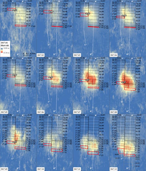
The monthly change of the area of deformation is presented in Figure 12 for the DInSAR measurements and in Figure 13 for the prediction model. The scale of the subsidence images is different for the two figures. The figures also show the location and values of the maximum subsidence for each month used in the later analyses. The numbers around the panels show the month and year of the starting date for the corresponding panel. The red polygons show the currently working panels. Two cross-sections through the area of deformation are drawn: Profile A′A′′ through longwall No. 6 and profile B′B′′ through longwall No. 5. The resulting profiles by month from radar measurements (Figure 14 and Figure 16) and from prediction models (Figure 15 and Figure 17) show the advancement of the subsidence in comparison with the ongoing work. The depth of the longwall is also presented, as the same cross-sections through the terrain and the longwall surface (Figure 9b,c) were performed; the profiles are presented on the bottom of Figure 14, Figure 15, Figure 16 and Figure 17.
Figure 12 explicitly shows that the DInSAR deformation is noisy, even when aggregated to a one-month period, and the deformation ambiguity is visible across the whole investigated domain. As a shift of the maximum subsidence towards the centre of the mining area is theoretically expected, the current extraction panels do not correlate with the maximum estimated subsidence, and the lag between the two is four (Figure 12; 2017.12) to ten (Figure 12; 2017.08) months. It is also visible that the main subsidence primarily affects the terrain above longwall No. 5 (profile B′B′′) and, to a much lesser extent, for longwall No. 6 (profile A′A′′).
The second set of figures (Figure 13) presents the modelled deformation. Obviously, the image is clearer, and there is no subsidence outside of the extraction panels. Subsidence is located directly under the extraction panel; therefore, the advancement of subsidence is directly correlated with the extraction progress. Each longwall has its own minimum deformation point. The maximum vertical deformation is 3–4 times larger than that obtained from DInSAR (Figure 12).
Figure 14, Figure 15, Figure 16 and Figure 17 provided for line A′A′′ and B′B′′ were analysed together, as they were prepared for the same dates. The shape of subsidence along these lines is different for DInSAR and the model. As mentioned, subsidence is initiated once the panel is extracted, but the main phase deformation lags by seven to ten months. No or little relation to the thickness of the seam are primarily observed. Moreover, the DInSAR deformation is more scattered around the mean solution, whereas the model deformation is a smoothed approximation of subsidence.
The maximal values of subsidence are also juxtaposed (see Figure 18) with the theoretical amount of extracted material from both longwalls as a function of the area of the panels and the thickness of the extracted coal seam.
Figure 18 shows good agreement of the DInSAR subsidence (blue line) with the averaged total extraction of the coal (black line) with an eight-month shift between extraction and deformation registration. This agreement is emphasised by correlation coefficient of 53%. Closer observation of the plot reveals particular discrepancies between the two compared graphs, which correspond to the DInSAR data with lower quality, namely those from January, February, November, and December 2017 (see Figure 4). Excluding these months leads to a correlation coefficient of 90%. Our further investigation will be focused on detailed study of these deviations during the winter season and the relation with the tropospheric artefacts in the radar signal. On the other hand, the model (red line in Figure 18) follows the extraction (black) line to a lesser degree (19%), especially at the ending four months of the comparable period.
Another analysed parameter is the vertical velocity of the extremal subsidence points in both the DInSAR and model data. Figure 19 shows that the DInSAR-based velocity (Equation (5)) is four-times smaller (5 mm/day) than the model-based velocity (20 mm/day). Both are linear with slightly increasing values for DInSAR velocity from 5–8 mm/day. In the case of the modelled velocity, the abrupt transition in October relates to the switch of maximum values between the two longwalls (Figure 13) and the difference in the time span for the month because of one missing ascending image in the beginning of October. Nevertheless, the main trend is of linear sinking through the whole area of mining activities during the phase of main subsidence. Calculated according to the Equation (6), the acceleration was frequently close to zero for the modelled point and also varies around zero for DInSAR. Two distinct features are visible: Negative acceleration (−0.10 mm/day) for DInSAR in September 2017 and positive acceleration (0.20 mm/day) for the model in October 2017.
4.3. Verification with Levelling
The reliability of the achieved results is validated with the data from two cycles of in-situ geodetic levelling carried out in the area of the coal seam 503 (Figure 7). The surface subsidence along six levelling lines was compared with the analogous DInSAR and predicted subsidence for the period between the levelling measurements in 2017, namely between April and October (Figure 20a–f).
Figure 20 shows that the model overestimates the subsidence for most of the levelling lines (see Figure 7 for lines locations)—for example, line 2′2′′ (Figure 20b), line 3′3′′ (Figure 20c), line 4′4′′ (Figure 20d), and line 6′6′′ (Figure 20f). Surprisingly, line number 1′1′′ (Figure 20a) traces through longwall No. 5, and the prediction of the subsidence does not represent the actual deformation, as the location of the subsidence trough was different. It is also interesting to note that line 5′5′′ (Figure 20e) stretching across longwall No. 6 shows mediocre deformation similar to that obtained from the DInSAR, whereas the model did not predict deformation in this area. The DInSAR is not in full agreement with levelling; however, it shows deformation trends similar to the levelling in all investigated lines. The deviations between DInSAR and levelling depends mostly on complex interconnections between subsidence and image acquisition (ascending and descending viewing angles) geometries. The correlations of the subsidence between the validation set of benchmarks and the remotely measured radar values and prediction model data, respectively, are presented by in Table 2.
The statistical study of the differences between the radar measured and modelled data compared to the levelling data for a set of 122 benchmarks within the investigated area in the Miechowice district is presented in Table 2. It shows a significant averaged difference (Equation (8)) corresponding to an off-set of about 20 cm in the modelling set, while, for the radar measurements, the error is about 4 cm.
The graphical representation of the correlation in Figure 21a shows a better fit with fewer outliers and a stronger correlation between the levelling and DInSAR-derived subsidence.
When the histograms (Figure 21b) for the two series are observed, the wider deviation of modelling subsidence and the skewness of its distribution can be noticed. The shape of the L-D histogram is closer to that of a normal distribution with the peak of the frequency between 0 and 0.20 m. After the Triangular Irregular Networks (TIN) generation based on the values in the benchmarks, a maximal difference is computed, resulting in 0.45 m at the west side and 0.31 m with opposite sign at the east side of the subsidence trough (Figure 21c). Between the levelling (L) and model (M) data, the maximal difference is 1.68 m (Figure 21d), while the highest frequency of the differences is in the range of minimum values (0 to 0.10 m; Figure 21b), which coincides with the benchmarks in the 2016 panels (Figure 21d).
5. Discussion
Coal mining deformations using InSAR have been intensively studied by several research groups in China and Australia. The results show the deformations in the area of interest due to nonlinearity (three phases of deformation). The rapid progress of deformation (5–20 mm/day) and large yearly deformations (exceeding 1.40 m/year) exceeds the capabilities of the PSI or SBAS methods. Hence, as in several other studies [14,17,19,21] related to the coal mine extraction, DInSAR was applied.
The most important lesson learned from high frequency (six days) DInSAR observation processing is that the quality of the observation varies over time (Figure 4) with a low percentage of overlay in the beginning of 2017 and uncertainties in deformations (Figure 10a and Figure 12). In general, when there are two consecutive interferograms with low quality, it may be considered that the common image has high perturbations due to atmospheric effects. To reduce the signal delay, different approaches may be performed, but the most preferable approach is by applying a weather model based on the information from global atmospheric models [40], models generated from GNSS observations [41], models that integrate both the weather forecast and GNSS tropospheric delay estimations [42], or spectrometer observations by systems like the Medium Resolution Imaging Spectrometer (MERIS) on-board the Envisat satellite or the Moderate Resolution Imaging Spectroradiometer (MODIS) on-board the Terra and Aqua satellites [43]. The aggregation to lower frequency observations, in line with the mining extraction plan, results in removing some of the lower coherence data, but highly tropospheric varying conditions still affect DInSAR deformations. Further studies using, for example, a generic atmospheric correction model [53,54], are required to quantify the effect of the troposphere on the obtained deformation. One of the reasons to aggregate the solution to one month was to reduce the impact of the troposphere.
The DInSAR-based extent of the subsidence received for the investigated case is reasonable. In the case of longwalls No. 5 and 6 from coal seam 503 of the Bytom-III mining area, the coal layer is 2.00 m in the area of the building of the Holy Cross Church; it is 2.30 m in the rest of the zone, which may produce a subsidence of 1.40–1.60 m to 1.61–1.84 m. It agrees well with the literature [55]. In the simplest situation, the theoretical expected subsidence due to the roof falling in longwall mining is 70% to 80% in the volume of the coal seam thickness. The amount of monthly vertical movement (Figure 18) correlates to the averaged material extraction. However, it must be noted also that the modelling assumptions must also consider the reactivation of old exploitations.
It is surprising to note that the subsidence model overestimates the maximum subsidence by 50% for the maximum subsidence point; however, we understand that safety precautions state that the model should present the worst-case scenario. There are two other significant discrepancies. The first is that the model of the maximum subsidence almost follows the current extraction panel, whereas in the DInSAR (Figure 12, Figure 13, Figure 14, Figure 15, Figure 16 and Figure 17) data, there is a substantial gap between Phase I and Phase II deformation. The shift between the two phases (see Figure 14, Figure 16 and Figure 18) covers approximately eight months, which corresponds to the phase of the main subsidence described in [17,18]. The second is the size and location of the subsidence trough. In the case of DInSAR deformations, these parameters are clearly under the influence of: Coal extraction parameters and 3D decomposition mis-modelling as described by several authors [14,56,57] that result in different impacts of horizontal deformation on vertical subsidence for data from ascending and descending orbits. The overestimated prediction values and locations of vertical displacements are in a relation with the time coefficients. The current study revealed the uncertainties in time factor determination and further study will be conducted taking into account the DInSAR results. Local geological conditions that may result in shifting the location of mining subsidence also have an influence [16,58]. The standard Knothe model idealises the ground deformation process which result in discrepancies between predicted and observed subsidence. As is described in [28], the uncertainties of the model parameters bring significant influence on the model accuracy. The coefficient of variability (standard deviation) for vertical displacements determined by [59] is equal to ±6%. The determined average standard deviation (difference between maximum values of predicted and observed vertical displacements) is equal to ±14% [2]. The result is referenced to 68% of probability, and, for a higher percentage of probability, it will result in higher deviations. The verification with levelling (Figure 20) shows that the trends in the subsidence and the shape of the subsidence trough are correctly represented by DInSAR. Thus, the radar results may be considered as effective for model parameter improvement. Still, the 3D decomposition aspect of the deformation will be further studied.
6. Conclusions
The current study aimed to provide more detailed information about the life cycle of the surface deformations caused by coal extractions. The DInSAR results have been proven reliable and accurate enough for monitoring the phase of main mine subsidence (−1.65 m over one year) with a −4 cm bias and 18.3 cm standard deviation when compared to levelling. The amount of detected surface vertical change is compatible with the amount of the extracted material and follows the stage of actual extraction for eight months, with up to 90% correlation coefficient. The radar data are within the range of the predefined predictive models, which ensures the minimum influence on the infrastructure and settlements. On the other hand, the new information that the radar measurements bring may improve the modelling strategy by adding an additional source for parameter determination. Another approach may involve the modelled horizontal displacements in the north-south direction in the formalisation of the 3D decomposition procedure. In this way, the solution for the vertical component may also be straightened. Significant enhancement will be achieved by applying the relevant procedure for the decrease of tropospheric artefacts in the radar signal and for georeferencing at particular GNSS stations.
Author Contributions
Conceptualization, M.I. and W.R.; methodology, M.I., W.R., A.B., P.P., and P.G.; software, A.B., W.R., K.S., and P.G.; validation, M.I. and P.P.; formal analysis, M.I. and K.S.; investigation, M.I. and P.P.; resources, P.P.; writing—original draft preparation, M.I., W.R., and P.P.; writing—review and editing, A.B., A.K., P.G., and K.S.; visualization, M.I.; supervision, A.B. and A.K.; project administration, W.R.; funding acquisition, W.R.
Funding
The presented investigation is part of the project EPOS-PL, European Plate Observing System POIR.04.02.00-14-A003/16, funded by the Operational Programme Smart Growth 2014–2020, Priority IV: Increasing the research potential, Action 4.2: Development of modern research infrastructure of the science sector and co-financed from European Regional Development Fund.
Acknowledgments
The Department of Węglokoks Kraj “Bobrek-Piekary” coal mine provided all documentation, including the maps and results of geodetic surveys.
Conflicts of Interest
The authors declare no conflict of interest.
References
- Zhu, X.; Guo, G.; Zha, J.; Chen, T.; Fang, Q.; Yang, X. Surface dynamic subsidence prediction model of solid backfill mining. Environ. Earth Sci. 2016, 75, 1007. [Google Scholar] [CrossRef]
- Kowalski, A. Deformacje Powierzchni w Górnośląskim Zagłębiu Węglowym [Surface Deformation in the Upper Silesian Coal Basin]; Główny Instytut Górnictwa: Katowice, Poland, 2015; ISBN 978-83-61126-93-5. [Google Scholar]
- Xu, C.-H.; Wang, J.-L.; Jing-Xiang, G.; Wang, J.; Hu, H. Precise point positioning and its application in mining deformation monitoring. Trans. Nonferr. Met. Soc. China 2011, 21, s499–s505. [Google Scholar] [CrossRef] [Green Version]
- Massonnet, D.; Rossi, M.; Carmona, C.; Adragna, F.; Peltzer, G.; Feigl, K.; Rabaute, T. The displacement field of the Landers earthquake mapped by radar interferometry. Nature 1993, 364, 138–142. [Google Scholar] [CrossRef]
- Stramondo, S.; Moro, M.; Doumaz, F.; Cinti, F.R. The 26 December 2003, Bam, Iran earthquake: Surface displacement from Envisat ASAR interferometry. Int. J. Remote Sens. 2005, 26, 1027–1034. [Google Scholar] [CrossRef]
- Samsonov, S.; Tiampo, K. Time series analysis of subsidence at Tauhara and Ohaaki geothermal fields, New Zealand, observed by ALOS PALSAR interferometry during 2007–2009. Can. J. Remote Sens. 2010, 36, S327–S334. [Google Scholar] [CrossRef]
- Yu, B.; Liu, G.; Li, Z.; Zhang, R.; Jia, H.; Wang, X.; Cai, G. Subsidence detection by TerraSAR-X interferometry on a network of natural persistent scatterers and artificial corner reflectors. Comput. Geosci. 2013, 58, 126–136. [Google Scholar] [CrossRef]
- Rucci, A.; Ferretti, A.; Monti Guarnieri, A.; Rocca, F. Sentinel 1 SAR interferometry applications: The outlook for sub millimeter measurements. Remote Sens. Environ. 2012, 120, 156–163. [Google Scholar] [CrossRef]
- Ferretti, A.; Prati, C.; Rocca, F. Nonlinear subsidence rate estimation using permanent scatterers in differential SAR interferometry. IEEE Trans. Geosci. Remote Sens. 2000, 38, 2202–2212. [Google Scholar] [CrossRef]
- Ferretti, A.; Prati, C.; Rocca, F. Permanent scatterers in SAR interferometry. IEEE Trans. Geosci. Remote Sens. 2001, 39, 8–20. [Google Scholar] [CrossRef] [Green Version]
- Ferretti, A.; Fumagalli, A.; Novali, F.; Prati, C.; Rocca, F.; Rucci, A. A new algorithm for processing interferometric data-stacks: SqueeSAR. IEEE Trans. Geosci. Remote Sens. 2011, 49, 3460–3470. [Google Scholar] [CrossRef]
- Berardino, P.; Fornaro, G.; Lanari, R.; Sansosti, E. A new algorithm for surface deformation monitoring based on small baseline differential SAR interferograms. IEEE Trans. Geosci. Remote Sens. 2002, 40, 2375–2383. [Google Scholar] [CrossRef]
- Hooper, A.; Zebker, H.; Segall, P.; Kampes, B. A new method for measuring deformation on volcanoes and other natural terrains using InSAR persistent scatterers. Geophys. Res. Lett. 2004, 31, 1–5. [Google Scholar] [CrossRef]
- Ng, A.H.-M.; Ge, L.; Yan, Y.; Li, X.; Chang, H.-C.; Zhang, K.; Rizos, C. Mapping accumulated mine subsidence using small stack of SAR differential interferograms in the Southern coalfield of New South Wales, Australia. Eng. Geol. 2010, 115, 1–15. [Google Scholar] [CrossRef]
- Crosetto, M.; Monserrat, O.; Cuevas-González, M.; Devanthéry, N.; Crippa, B. Persistent Scatterer Interferometry: A review. ISPRS J. Photogramm. Remote Sens. 2016, 115, 78–89. [Google Scholar] [CrossRef] [Green Version]
- Borecki, M. Ochrona Powierzchni Przed Szkodami Górniczymi [Surface Protection against Mining Damage]; Wydawnictwo Śląsk: Katowice, Poland, 1980; pp. 1–967. [Google Scholar]
- Perski, Z. ERS InSAR data for Geological Interpretation of Mining Subsidence in Upper Silesian Coal Basin in Poland. In Proceedings of the FRINGE’99 2nd International Workshop on SAR Interferometry, Liege, Belgium, 10–12 November 1999. [Google Scholar]
- Jarosz, A.; Karmis, M.; Sroka, A. Subsidence development with time—Experiences from longwall operations in the Appalachian coalfield. Int. J. Min. Geol. Eng. 1990, 8, 261–273. [Google Scholar] [CrossRef]
- Ng, A.H.-M.; Ge, L.; Du, Z.; Wang, S.; Ma, C. Satellite radar interferometry for monitoring subsidence induced by longwall mining activity using Radarsat-2, Sentinel-1 and ALOS-2 data. Int. J. Appl. Earth Obs. Geoinf. 2017, 61, 92–103. [Google Scholar] [CrossRef]
- Przyłucka, M.; Herrera, G.; Graniczny, M.; Colombo, D.; Béjar-Pizarro, M. Combination of conventional and advanced DInSAR to monitor very fast mining subsidence with TerraSAR-X data: Bytom City (Poland). Remote Sens. 2015, 7, 5300–5328. [Google Scholar] [CrossRef]
- Ma, C.; Cheng, X.; Yang, Y.; Zhang, X.; Guo, Z.; Zou, Y. Investigation on mining subsidence based on multi-temporal InSAR and time-series analysis of the small baseline subset—Case study of working faces 22201-1/2 in Bu’ertai mine, Shendong coalfield, China. Remote Sens. 2016, 8, 951. [Google Scholar] [CrossRef]
- Zhou, Y.; Stein, A.; Molenaar, M. Integrating interferometric SAR data with levelling measurements of land subsidence using geostatistics. Int. J. Remote Sens. 2003, 24, 3547–3563. [Google Scholar] [CrossRef]
- Fuhrmann, T.; Caro Cuenca, M.; Knöpfler, A.; Van Leijen, F.J.; Mayer, M.; Westerhaus, M.; Hanssen, R.F.; Heck, B. Combining InSAR, Levelling and GNSS for the Estimation of 3D Surface Displacements; European Space Agency: Paris, France, 2015; Volume SP-731. [Google Scholar]
- Chen, L.; Zhang, L.; Tang, Y.; Zhang, H. Analysis of mining-induced subsidence prediction by exponent Knothe model combined with InSAR and levelling. ISPRS Ann. Photogramm. Remote Sens. Spat. Inf. Sci. 2018, IV-3, 53–59. [Google Scholar] [CrossRef]
- Perski, Z. Applicability of ERS-1 and ERS-2 InSAR for land subsidence monitoring in the Silesian coal mining region, Poland. Int. Arch. Photogramm. Remote Sens. 1998, XXXII, 555–558. [Google Scholar]
- Kwiatek, J. Ochrona Obiektów Budowlanych na Terenach Górniczych [Protection of Buildings in Mining Areas]; Wydawnictwo Śląsk: Katowice, Poland, 1997. [Google Scholar]
- Perski, Z.; Jura, D. Identification and measurement of mining subsidence with SAR interferometry: Potentials and limitations. In Proceedings of the 11th International FIG Symposium on Deformation Measurements, Santorini, Greece, 25–28 May 2003. [Google Scholar]
- Blachowski, J.; Milczarek, W.; Stefaniak, P. Deformation information system for facilitating studies of mining-ground deformations, development, and applications. Nat. Hazards Earth Syst. Sci. 2014, 14, 1677–1689. [Google Scholar] [CrossRef] [Green Version]
- Gruszczyński, W.; Niedojadło, Z.; Mrocheń, D. Influence of model parameter uncertainties on forecasted subsidence. Acta Geodyn. Geomater. 2018, 15, 211–228. [Google Scholar] [CrossRef]
- Li, P.; Peng, D.; Tan, Z.; Deng, K. Study of probability integration method parameter inversion by the genetic algorithm. Int. J. Min. Sci. Technol. 2017, 27, 1073–1079. [Google Scholar] [CrossRef]
- Knothe, S. Wpływ czasu na kształtowanie się niecki osiadania [Influence of time on the formation of subsidence trough]. Arch. Górnictwa i Hut. 1953, 1, 51. [Google Scholar]
- Knothe, S. Prognozowanie Wpływów Eksploatacji Górniczej [Forecasting the Impact of Mining Exploitation]; Wydawnictwo Śląsk: Katowice, Poland, 1984. [Google Scholar]
- Kowalski, A. Nieustalone Górnicze Deformacje Powierzchni w Aspekcie Dokładności Prognoz [Dynamic Mining Surface Deformations in the Aspect of Forecast Accuracy]; Głównego Instytutu Górnictwa: Katowice, Poland, 2007. [Google Scholar]
- Yang, Z.F.; Li, Z.W.; Zhu, J.J.; Hu, J.; Wang, Y.J.; Chen, G.L. Analysing the law of dynamic subsidence in mining area by fusing InSAR and leveling measurements. Int. Arch. Photogramm. Remote Sens. Spat. Inf. Sci. ISPRS Arch. 2013, 40, 163–166. [Google Scholar] [CrossRef]
- Iannacone, J.P.; Alessandro, C.; Berti, M.; Morgan, J.; Falorni, G. Characterization of longwall mining induced subsidence by means of automated analysis of InSAR time-series. Eng. Geol. Soc. Territ. 2015, 5, 973–977. [Google Scholar]
- Sun, Q.; Li, Z.W.; Ding, X.L.; Zhu, J.J.; Hu, J. Multi-temporal InSAR data fusion for investigating mining subsidence. In Proceedings of the 2011 International Symposium on Image and Data Fusion, Tengchong, China, 9–11 August 2011. [Google Scholar]
- Coulthard, M.A. Applications of numerical modelling in underground mining and construction. Geotech. Geol. Eng. 1999, 17, 373–385. [Google Scholar] [CrossRef]
- Shahriar, K.; Amoushahi, S.; Arabzadeh, M. Prediction of surface subsidence due to inclined very shallow coal seam mining using FDM. In Proceedings of the Coal Operators’ Conference, Wollongong, Australia, 12–13 February 2009; pp. 130–139. [Google Scholar]
- Rodriguez, E.; Morris, C.S.; Belz, J.E.; Chapin, E.C.; Martin, J.M.; Daffer, W.; Hensley, S. An Assessment of the SRTM Topographic Products; Technical Report JPL D-31639; Jet Propulsion Laboratory: Pasadena, CA, USA, 2005. [Google Scholar]
- Chen, C.W.; Zebker, H.A. Network approaches to two-dimensional phase unwrapping: Intractability and two new algorithms. J. Opt. Soc. Am. A 2000, 17, 401–414. [Google Scholar] [CrossRef]
- Duchon, J. Interpolation des fonctions de deux variables suivant le principe de la flexion des plaques minces [Interpolation of the functions of two variables according to the principle of thin-plate spline]. Revue française d'automatique informatique recherche opérationnelle Analyse numérique 1976, 10, 5–12. [Google Scholar] [CrossRef]
- Thin-Plate Spline Interpolation. Available online: https://doi.org/10.1007/s00190-019-01240-2 (accessed on 27 February 2019).
- Zheng, M.; Deng, K.; Fan, H.; Huang, J. Monitoring and analysis of mining 3D deformation by multi-platform SAR images with the probability integral method. Front. Earth Sci. 2019, 13, 169–179. [Google Scholar] [CrossRef]
- Haghshenas Haghighi, M.; Motagh, M. Sentinel-1 InSAR over Germany: Large-scale interferometry, atmospheric effects, and ground deformation mapping. ZfV-Zeitschrift für Geodäsie Geoinformation und Landmanagement 2017, 142, 245–256. [Google Scholar]
- Jones, E.; Oliphant, E.; Peterson, P. SciPy: Open Source Scientific Tools for Python. Available online: http://www.scipy.org/ (accessed on 16 December 2018).
- Geospatial Data Abstraction Library (GDAL/OGR) Contributors. GDAL/OGR Geospatial Data Abstraction Software Library. Available online: http://gdal.org (accessed on 18 December 2018).
- Gruchlik, P. Zastosowanie Modeli Reologicznych do Opisu Nieustalonych Deformacji Powierzchni [Application of Rheological Models to Describe Dynamic Surface Deformations]; Główny Instytutu Górnictwa: Katowice, Poland, 2003. [Google Scholar]
- Jędrzejec, E. Wersja 5.0 programu Szkody do prognozowania poeksploatacyjnych deformacji górotworu [Version 5.0 of the Szkody programme for forecasting post extraction ground deformation]. WUG Bezpieczeństwo Pracy i Ochrona Środowiska w Górnictwie 2008, 2, 15–19. [Google Scholar]
- World Energy Council: Coal in Poland. Available online: https://www.worldenergy.org/data/resources/country/poland/coal/ (accessed on 29 October 2018).
- Wirth, P. Post-Mining Regions in Central Europe—Problem, Potentials, Possibilities; Wirth, P., Černič Mali, B., Fischner, W., Eds.; Oekom: München, Germany, 2012. [Google Scholar]
- Alves Dias, P.; Kanellopoulos, K.; Medarac, H.; Kapetaki, Z.; Miranda-Barbosa, E.; Shortall, R.; Czako, V.; Telsnig, T.; Vazquez-Hernandez, C.; Lacal Arántegui, R.; et al. EU Coal Regions: Opportunities and Challenges Ahead; European Union: Luxembourg, 2018. [Google Scholar]
- Perski, Z. The interpretation of ERS-1 and ERS-2 InSAR data for the mining subsidence monitoring in Upper Silesian Coal Basin, Poland. Int. Arch. Photogramm. Remote Sens. 2000, XXXIII, 1137–1141. [Google Scholar]
- Volkmer, G. Coal deposits of Poland, including discussion about the degree of peat consolidation during lignite formation. TU Bergakad. Freib. 2006, 1–11. Available online: http://docplayer.net/47498077-Coal-deposits-of-poland-including-discussion-about-the-degree-of-peat-consolidation-during-lignite-formation.html (accessed on 15 January 2019).
- Bekaert, D.P.S.; Walters, R.J.; Wright, T.J.; Hooper, A.J.; Parker, D.J. Statistical comparison of InSAR tropospheric correction techniques. Remote Sens. Environ. 2015, 170, 40–47. [Google Scholar] [CrossRef] [Green Version]
- Yu, C.; Li, Z.; Penna, N.T.; Crippa, P. Generic Atmospheric Correction Model for Interferometric Synthetic Aperture Radar Observations. J. Geophys. Res. Solid Earth 2018, 123, 9202–9222. [Google Scholar] [CrossRef]
- Mróz, M.; Perski, Z. The integration of optical and InSAR data for land subsidence monitoring and its impact on environment of the Upper Silesian Coal Basin. In Proceedings of the Geoinformation for European-Wide Integration, 22nd Symposium of the European Association of Remote Sensing Laboratories, Prague, Czech Republic, 4–6 June 2003; MillPress: Bethlehem, PA, USA; pp. 621–624. [Google Scholar]
- Qu, C.; Shan, X.; Zhao, D.; Zhang, G.; Song, X. Relationships between InSAR Seismic Deformation and Fault Motion Sense, Fault Strike, and Ascending/Descending Modes. Acta Geol. Sin. 2017, 91, 93–108. [Google Scholar] [CrossRef] [Green Version]
- Pagli, C.; Wang, H.; Wright, T.J.; Calais, E.; Lewi, E. Current plate boundary deformation of the Afar rift from a 3-D velocity field inversion of InSAR and GPS. J. Geophys. Res. Solid Earth 2014, 119, 8562–8575. [Google Scholar] [CrossRef] [Green Version]
- Popiołek, E. Ochrona Terenów Górniczych [Protection of Mining Areas]; Wydawnictwo Akademii Górniczo-Hutniczej im. Stanisława Staszica: Warsaw, Poland, 2009; ISBN 978-83-7464-229-3. [Google Scholar]
Figure 1.
Differential satellite radar interferometry (DInSAR) processing and post-processing flow.

Figure 2.
Ascending (blue) and descending (green) orbit footprints of Sentinel-1 data used in this study over the territory of the Polish part of Upper Silesian Coal Basin (USCB).
Figure 2.
Ascending (blue) and descending (green) orbit footprints of Sentinel-1 data used in this study over the territory of the Polish part of Upper Silesian Coal Basin (USCB).

Figure 3.
Procedure for evaluation of the quality of DInSAR displacement maps.

Figure 4.
Quality assessment of the ascending (Asc) and descending (Desc) interferograms. The values in the bars show the perpendicular baselines of each interferogram.
Figure 4.
Quality assessment of the ascending (Asc) and descending (Desc) interferograms. The values in the bars show the perpendicular baselines of each interferogram.

Figure 5.
An example of trend removal for the descending orbit, displacements between 2nd and 8th of January 2017: Original data (left), trend function (middle), and smoothed data (right). The example is the local (image) coordinate system; deformation values in [m]. Please note different deformation scales in the original and smoothed images.

Figure 6.
Distribution of steady and dynamic subsidence [2].
Figure 6.
Distribution of steady and dynamic subsidence [2].

Figure 7.
Levelling network in the Miechowice district (left) and the chosen reference dates for each levelling cycle (right).
Figure 7.
Levelling network in the Miechowice district (left) and the chosen reference dates for each levelling cycle (right).

Figure 8.
Population density in Poland for 2011 (left), according to the Central Statistical Office, and in the USCB (right).
Figure 8.
Population density in Poland for 2011 (left), according to the Central Statistical Office, and in the USCB (right).

Figure 9.
(a) The range of the investigated longwalls No. 5 and 6 from seam 503 of the Bytom-III mining area located in the northern part of USCB (see Figure 8 right); (b) depth of the longwalls with respect to the sea level. The numbers represent the starting date (YY.MM) for extractions from the corresponding panel; (c) terrain elevation above the mined area from Shuttle Radar Topography Mission (SRTM) Digital Elevation Model (DEM).

Figure 10.
Cumulative surface changes for the entire year of 2017: (a) Displacements in the east-west direction from DInSAR, (b) from the model, (c) vertical subsidence derived from DInSAR, and (d) from the model.
Figure 10.
Cumulative surface changes for the entire year of 2017: (a) Displacements in the east-west direction from DInSAR, (b) from the model, (c) vertical subsidence derived from DInSAR, and (d) from the model.

Figure 11.
Areal resemblance between Differential satellite radar interferometric (DInSAR) measured and expected range of surface deformation; Left: Example for March; Right: Percentage in the overlay area.
Figure 11.
Areal resemblance between Differential satellite radar interferometric (DInSAR) measured and expected range of surface deformation; Left: Example for March; Right: Percentage in the overlay area.

Figure 12.
Monthly advancement of coal extraction presented by the red panels and main subsidence presented by images according to the DInSAR measurements. Profiles along the line A′A′′ are shown in Figure 14 and along the line B′B′′ in Figure 16.

Figure 13.
Monthly advancement of coal extraction presented by the red panels and the main subsidence presented by images according to the prediction models based on the Knothe–Budryk theory. Profiles along the line A′A′′ are shown in Figure 15 and along the line B′B′′ in Figure 17.

Figure 14.
Profile A′A′′ (longwall No. 6) through the DInSAR: The blue curves show the vertical subsidence by month in 2017. The grey vertical lines show the location of the panels of extractions according to the starting date (above each graph). The shaded area is the currently extracted panel for the presented month. On the bottom of the figure, profiles of the DEM surface and depth and thickness of coal seam are presented.

Figure 15.
Profile A′A′′ (longwall No. 6) through the models. The red curves show the vertical subsidence by month in 2017. On the bottom of the figure, profiles of the DEM surface and depth and thickness of coal seam are presented.
Figure 15.
Profile A′A′′ (longwall No. 6) through the models. The red curves show the vertical subsidence by month in 2017. On the bottom of the figure, profiles of the DEM surface and depth and thickness of coal seam are presented.

Figure 16.
Profile B′B′′ (longwall No. 5) through the DInSAR. The blue curves show the vertical subsidence by month in 2017. On the bottom of the figure, profiles of the DEM surface and depth and thickness of coal seam are presented.
Figure 16.
Profile B′B′′ (longwall No. 5) through the DInSAR. The blue curves show the vertical subsidence by month in 2017. On the bottom of the figure, profiles of the DEM surface and depth and thickness of coal seam are presented.

Figure 17.
Profile B′B′′ (longwall No. 5) through the models. The red curves show the vertical subsidence by month in 2017. On the bottom of the figure, profiles of the DEM surface and depth and thickness of coal seam are presented.
Figure 17.
Profile B′B′′ (longwall No. 5) through the models. The red curves show the vertical subsidence by month in 2017. On the bottom of the figure, profiles of the DEM surface and depth and thickness of coal seam are presented.

Figure 18.
Amount of maximal subsidence by months detected by DInSAR (blue) and predicted from the model (red), compared with the estimated material extraction from coal seam 503. The black axis values on the right and bottom represent the subsidence and corresponding dates, respectively. The grey axis values on the left and above the graph relate to the amount of the extracted material and the time for these events.

Figure 19.
Velocity (left) and acceleration (right) of the subsidence for the extremal points by months.
Figure 19.
Velocity (left) and acceleration (right) of the subsidence for the extremal points by months.

Figure 20.
Comparison of the subsidence [in meter] along the levelling lines from Figure 7 between DInSAR results, levelling and predicted by the model data: (a) profile along levelling line 1′1′′, (b) profile along levelling line 2′2′′, (c) profile along levelling line 3′3′′, (d) profile along levelling line 4′4′′, (e) profile along levelling line 5′5′′, (f) profile along levelling line 6′6′′

Figure 21.
(a) Correlation between subsidence from the levelling (vertical axis) and DInSAR (blue) and model (red) along the horizontal axis; (b) histogram of the distribution of errors between subsidence derived from levelling (L), DInSAR (D), and modelling (M); and fields of errors for (c) L-D and (d) L-M.


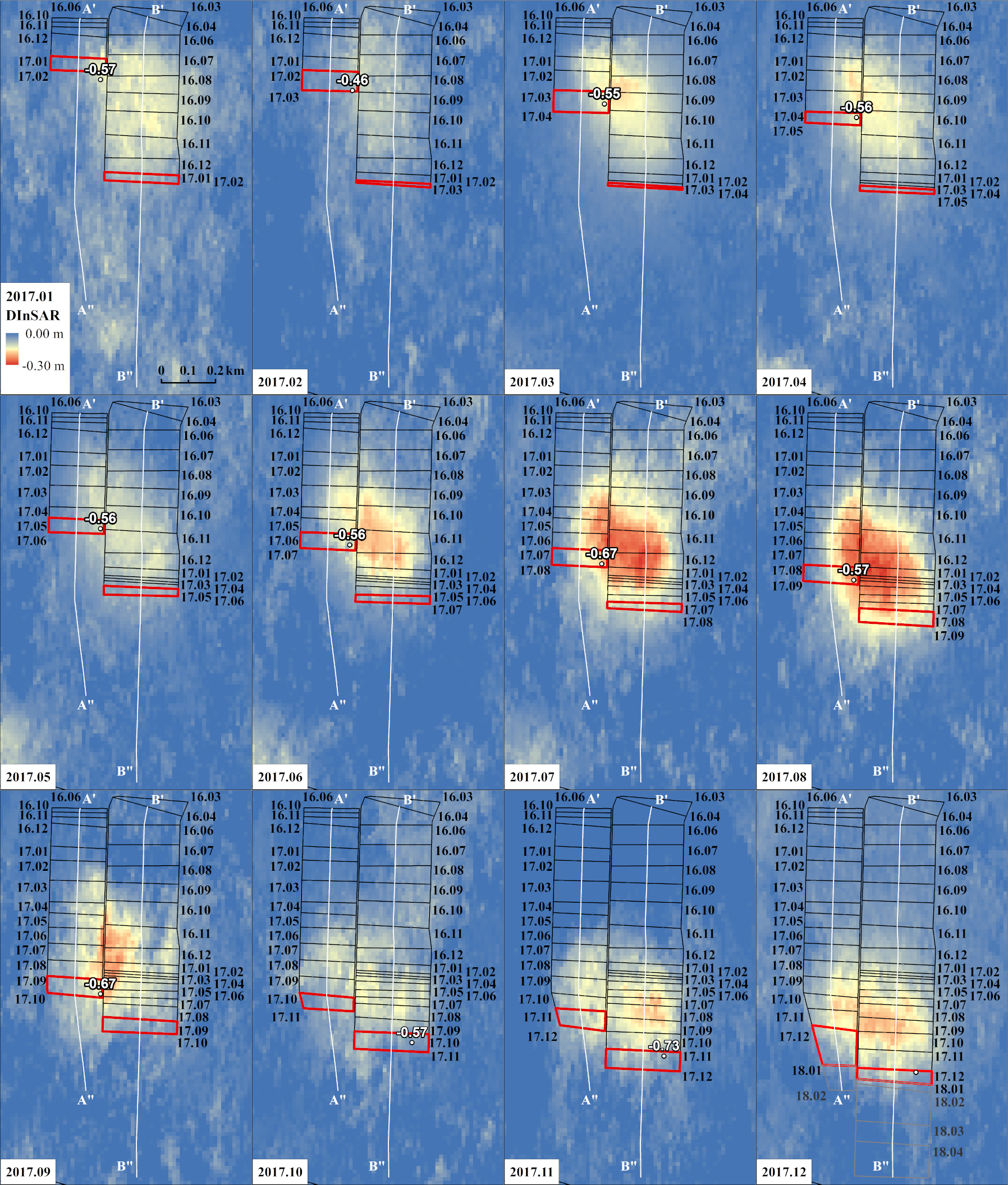
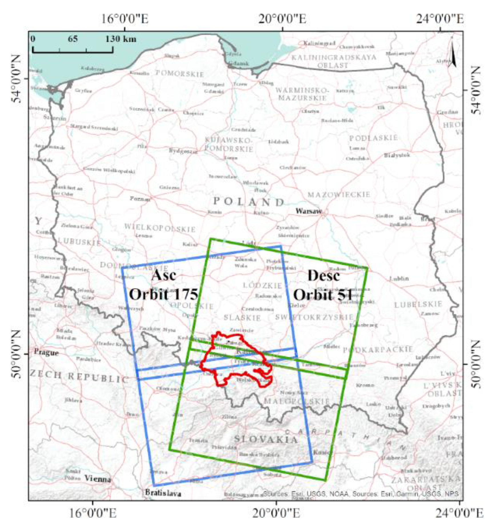
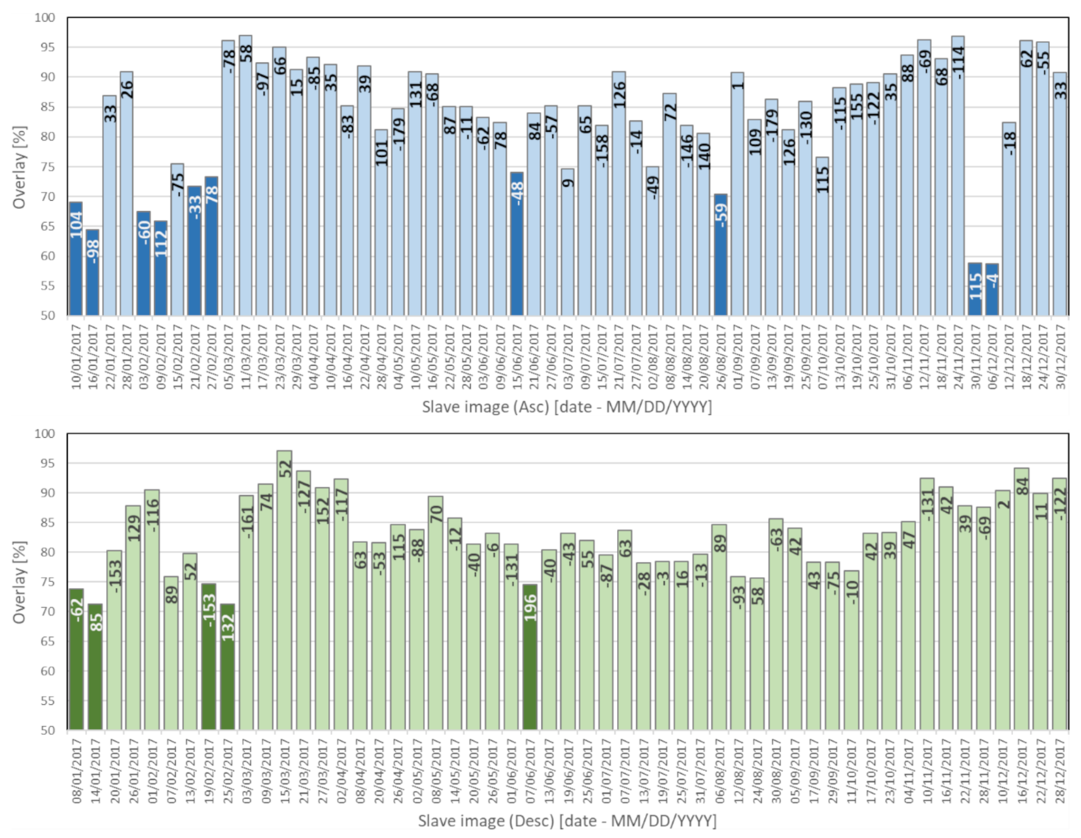
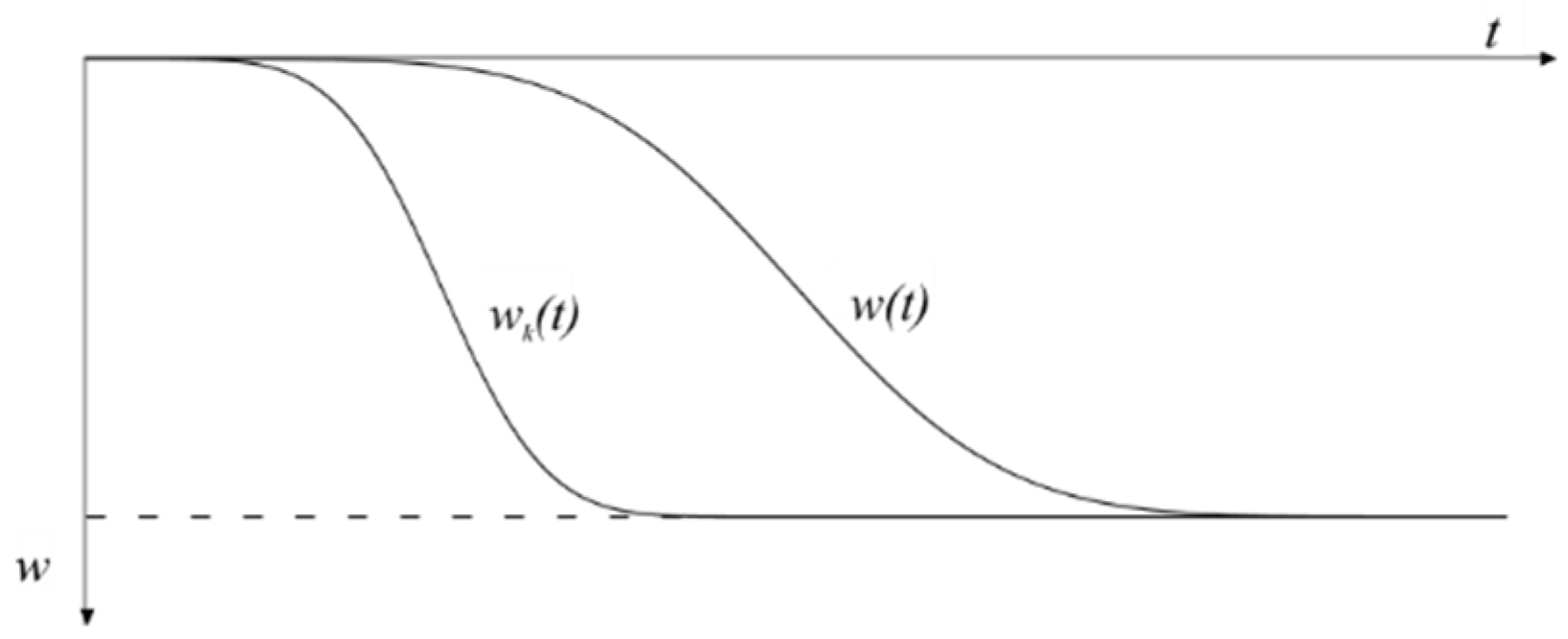
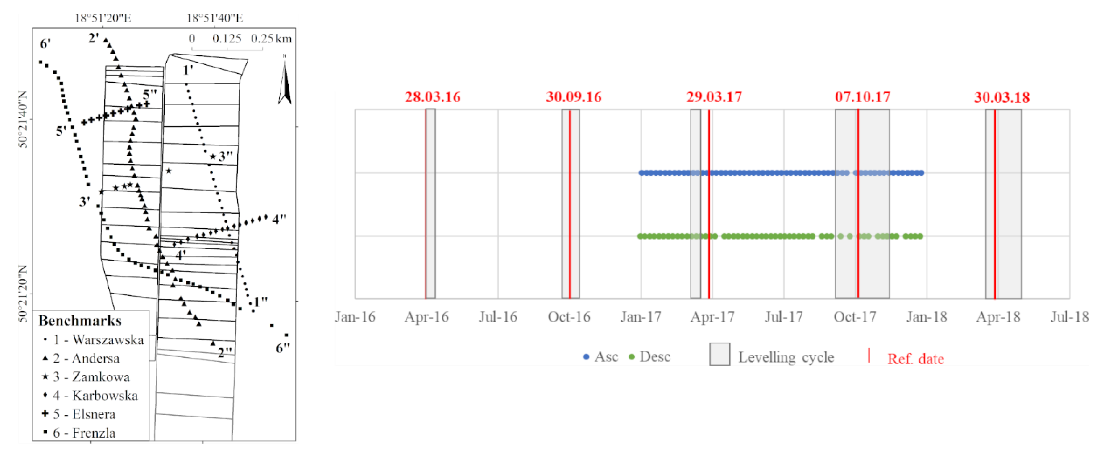
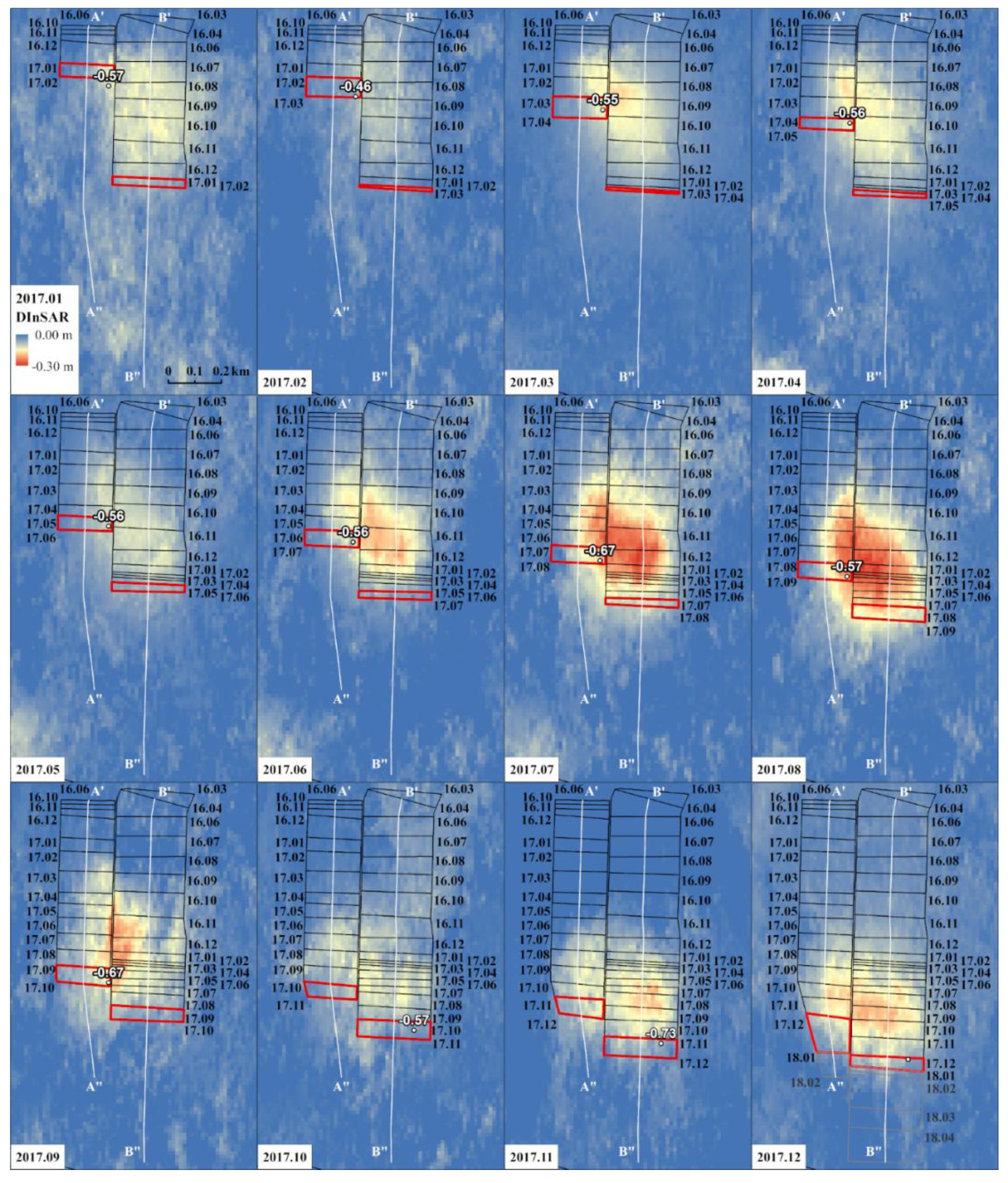
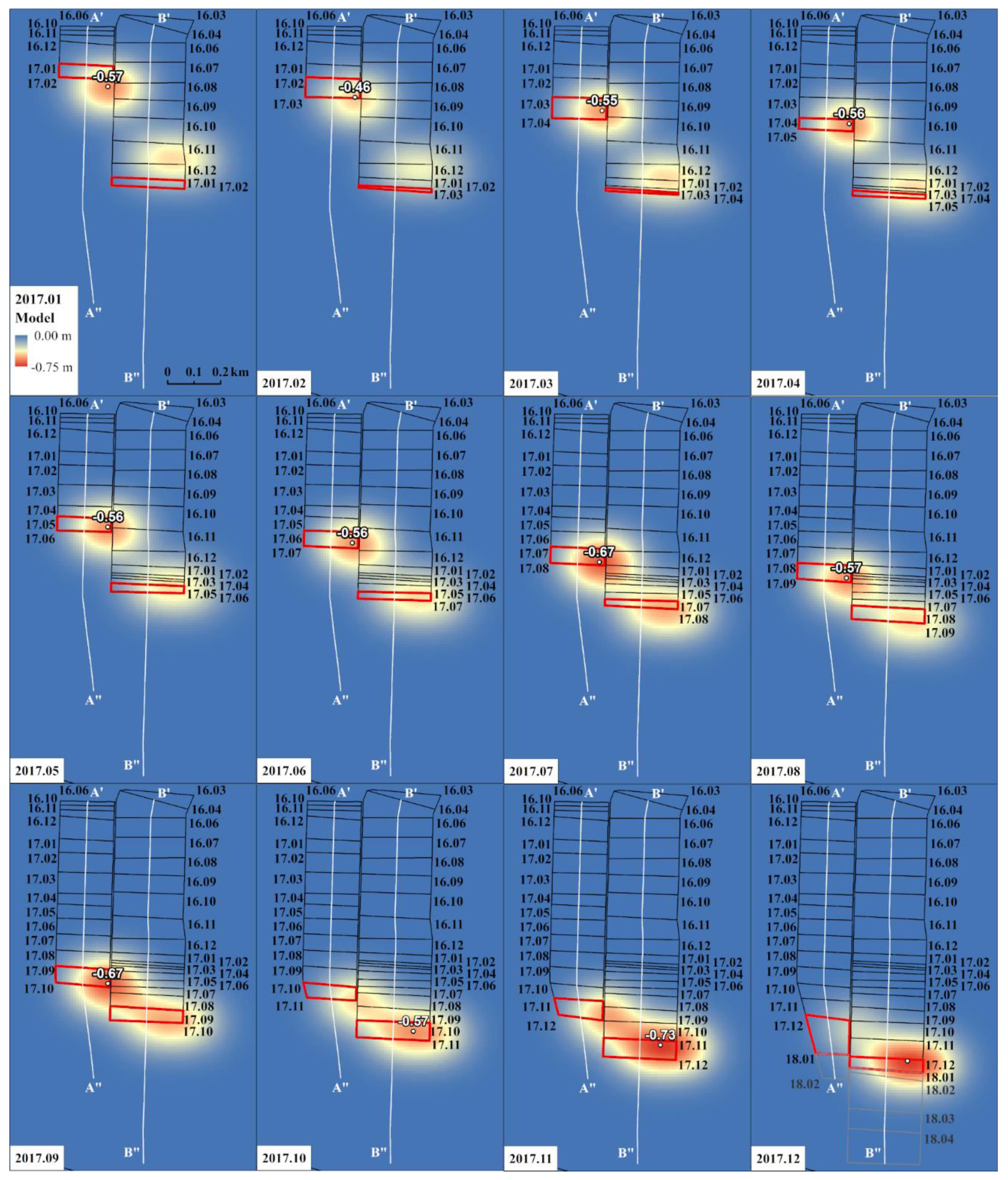
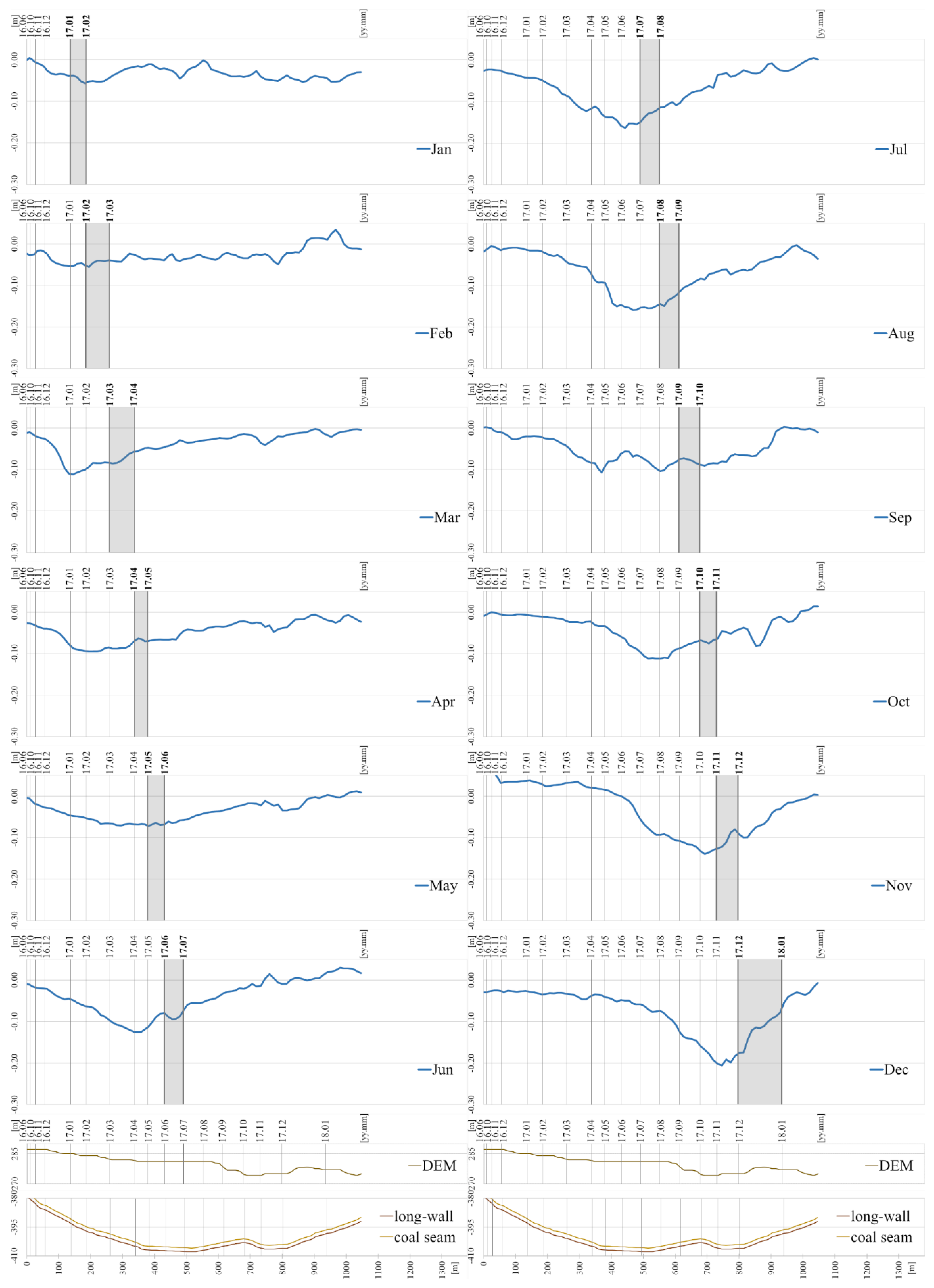
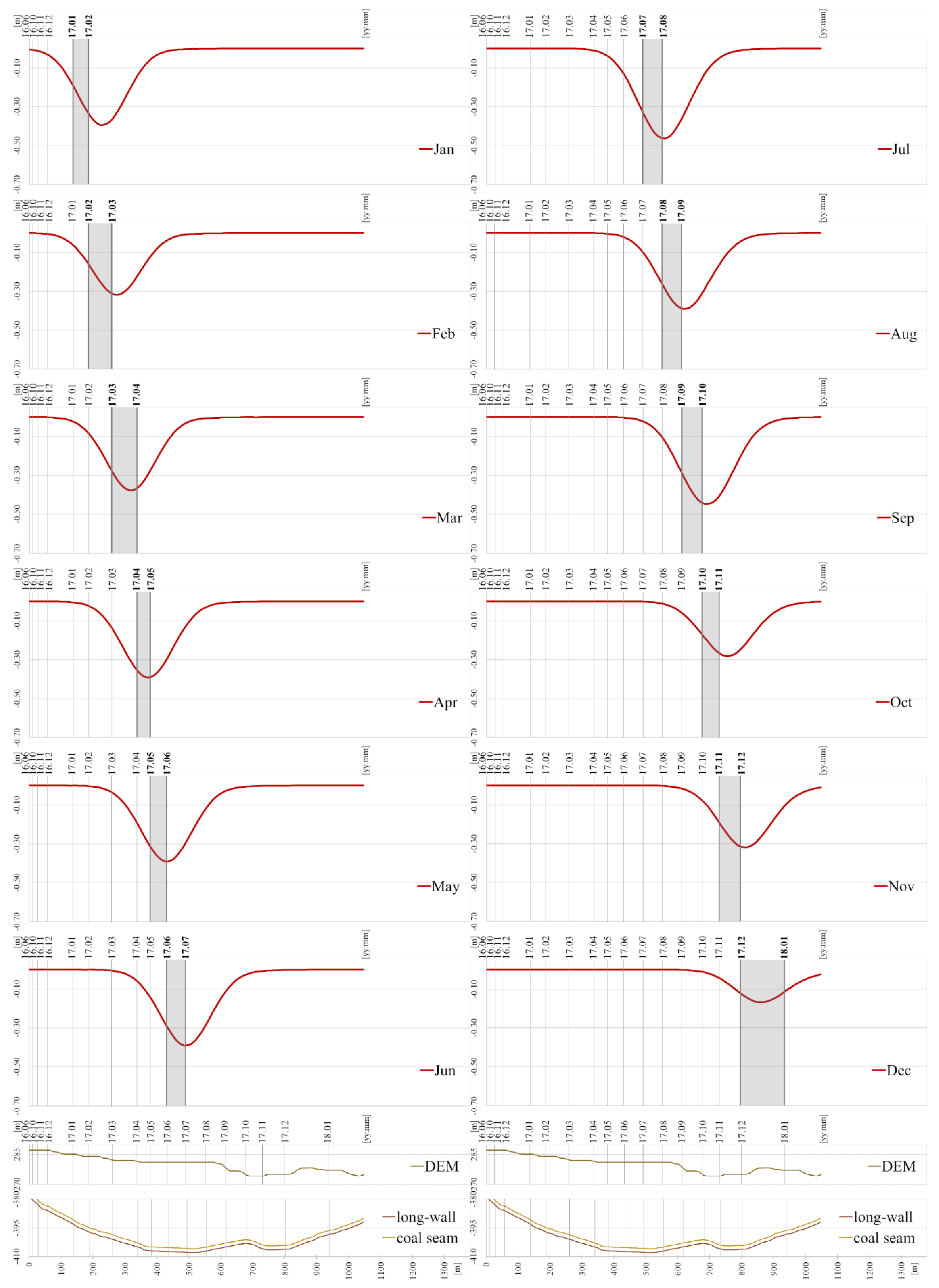
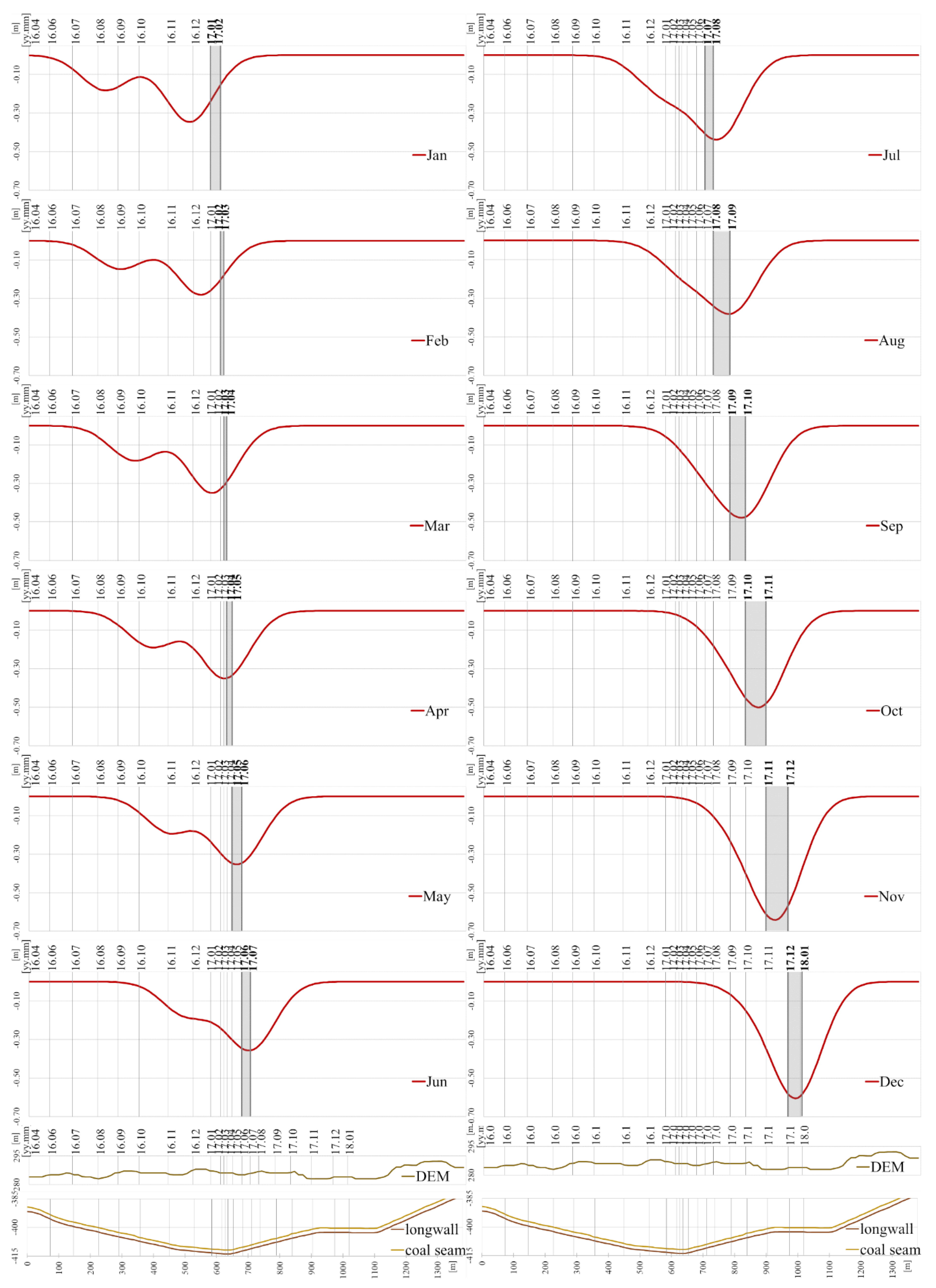
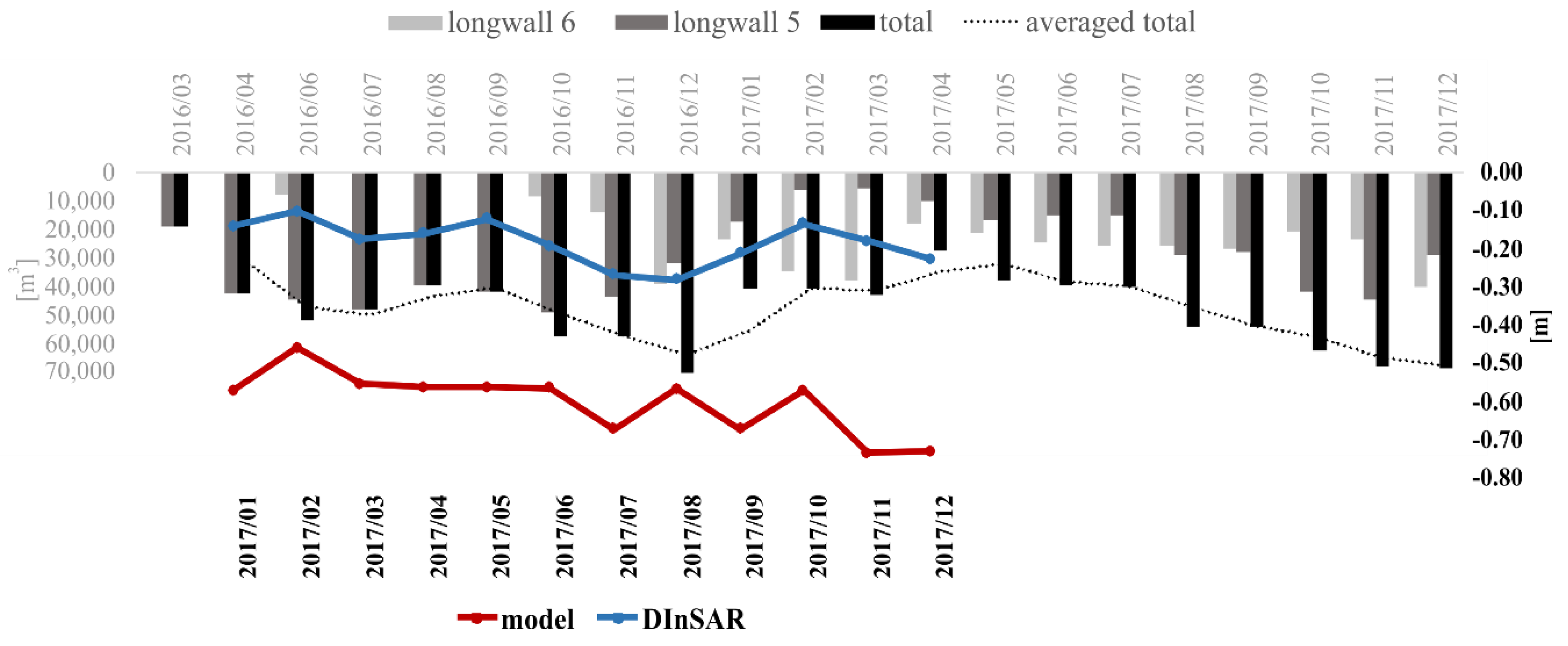
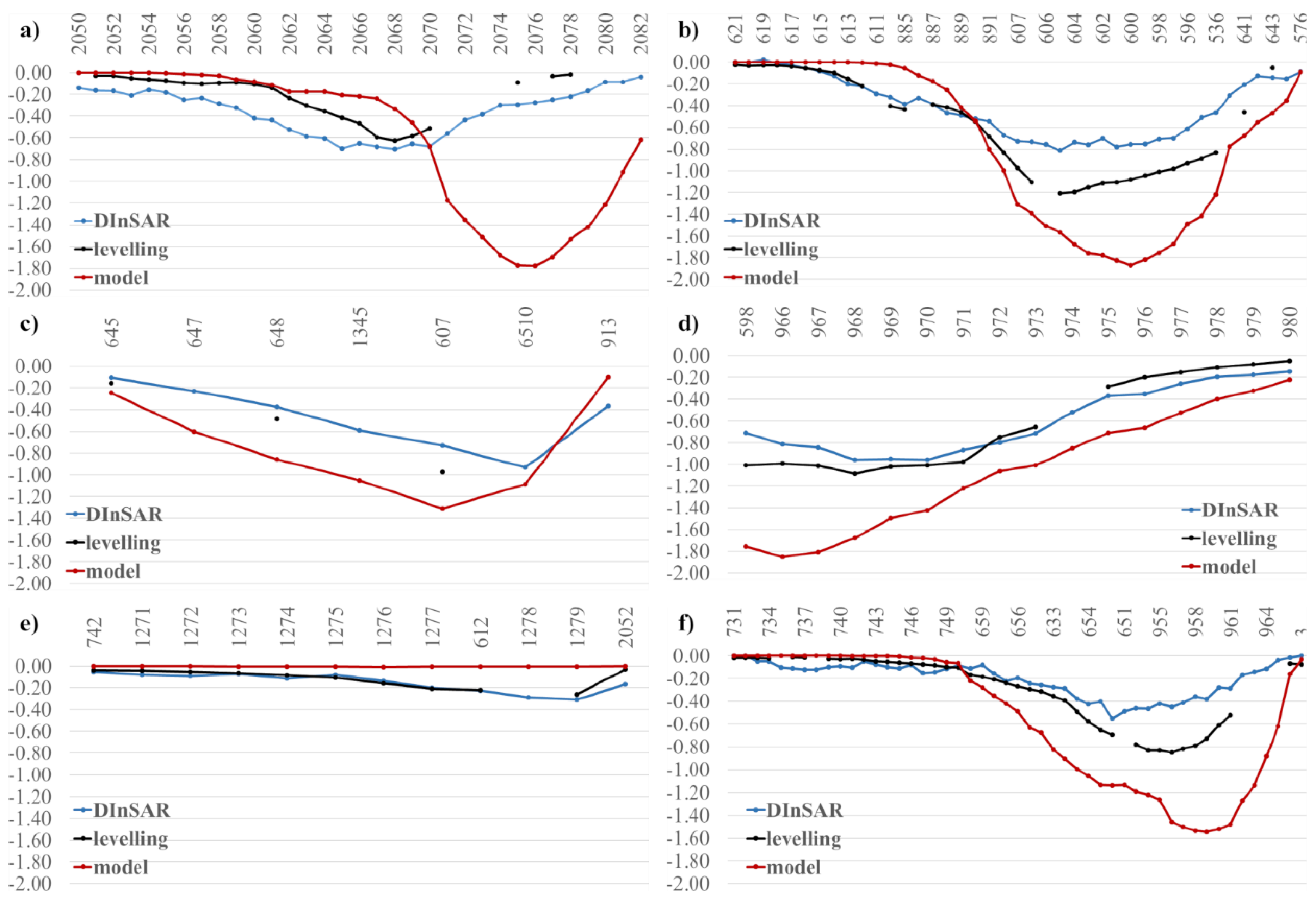
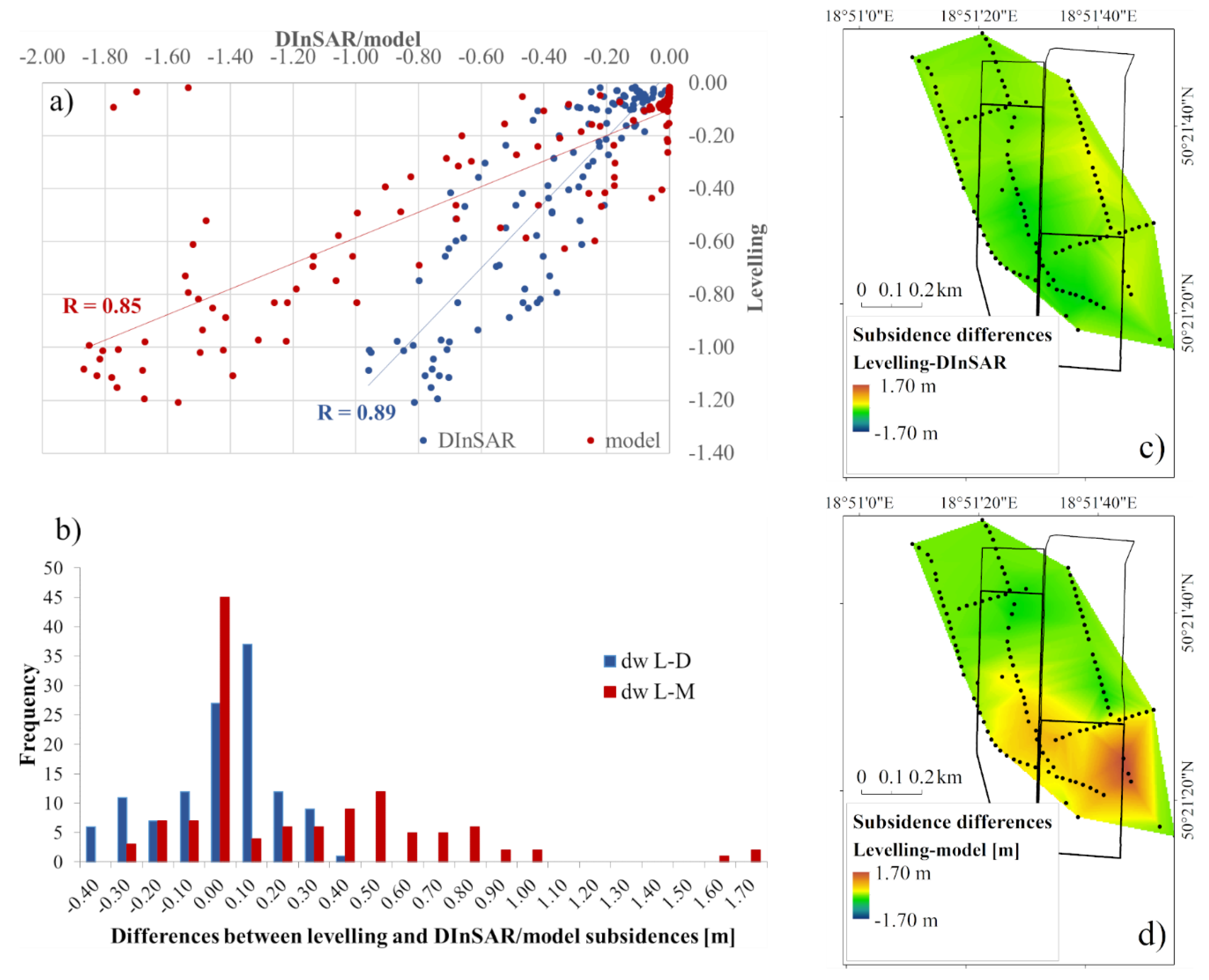
Table 1.
Dataset of determined parameters of the Knothe–Budryk theory and standard deviation (Std) values of matching for exploitation of the 503 seam with longwalls No. 5 and 6.
Table 1.
Dataset of determined parameters of the Knothe–Budryk theory and standard deviation (Std) values of matching for exploitation of the 503 seam with longwalls No. 5 and 6.
| Drawn Line (Profile Lines from Figure 7 in Brackets) | Determined Subsidence Parameters from the Knothe–Budryk Theory | Std of Subsidence Parameters Matching , mm | ||
|---|---|---|---|---|
| Subsidence Factor | Rock Mass Parameter | Exploitation Rim , m | ||
| no 1 (2′-2′′) | 1.13 | 4.5 | 90 | 235 |
| no 2 (1′-1′′) | 1.00 | 3.1 | 90 | 91 |
| no 3 (4′-4′′, 2′-2′′, 6′-6′′) | 1.14 | 2.7 | 50 | 257 |
| no 4 (6′-6′′) | 1.25 | 3.3 | 90 | 86 |
| no 5 (5′-5′′, 6′-6′′, 4′-4′′) | 1.08 | 2.9 | 90 | 281 |
Table 2.
Statistical assessment of the DInSAR (D) and model (M) data compared to the verification data from levelling (L).
Table 2.
Statistical assessment of the DInSAR (D) and model (M) data compared to the verification data from levelling (L).
| L-D | 0.89 | -0.04 | 0.183 |
| L-M | 0.85 | 0.20 | 0.388 |
© 2019 by the authors. Licensee MDPI, Basel, Switzerland. This article is an open access article distributed under the terms and conditions of the Creative Commons Attribution (CC BY) license (http://creativecommons.org/licenses/by/4.0/).
Share and Cite
MDPI and ACS Style
Ilieva, M.; Polanin, P.; Borkowski, A.; Gruchlik, P.; Smolak, K.; Kowalski, A.; Rohm, W. Mining Deformation Life Cycle in the Light of InSAR and Deformation Models. Remote Sens. 2019, 11, 745. https://doi.org/10.3390/rs11070745
AMA Style
Ilieva M, Polanin P, Borkowski A, Gruchlik P, Smolak K, Kowalski A, Rohm W. Mining Deformation Life Cycle in the Light of InSAR and Deformation Models. Remote Sensing. 2019; 11(7):745. https://doi.org/10.3390/rs11070745
Chicago/Turabian StyleIlieva, Maya, Piotr Polanin, Andrzej Borkowski, Piotr Gruchlik, Kamil Smolak, Andrzej Kowalski, and Witold Rohm. 2019. "Mining Deformation Life Cycle in the Light of InSAR and Deformation Models" Remote Sensing 11, no. 7: 745. https://doi.org/10.3390/rs11070745
Note that from the first issue of 2016, this journal uses article numbers instead of page numbers. See further details here.