Using 1st Derivative Reflectance Signatures within a Remote Sensing Framework to Identify Macroalgae in Marine Environments


School of Water, Energy and Environment, Cranfield University, College Road, Cranfield MK43 0AL, UK
*
Author to whom correspondence should be addressed.
Remote Sens. 2019, 11(6), 704; https://doi.org/10.3390/rs11060704
Submission received: 28 January 2019
/
Revised: 19 March 2019
/
Accepted: 20 March 2019
/
Published: 23 March 2019
(This article belongs to the Special Issue Novel Advances in Aquatic Vegetation Monitoring in Ocean, Lakes and Rivers)
Abstract
:Macroalgae blooms (MABs) are a global natural hazard that are likely to increase in occurrence with climate change and increased agricultural runoff. MABs can cause major issues for indigenous species, fish farms, nuclear power stations, and tourism activities. This project focuses on the impacts of MABs on the operations of a British nuclear power station. However, the outputs and findings are also of relevance to other coastal operators with similar problems. Through the provision of an early-warning detection system for MABs, it should be possible to minimize the damaging effects and possibly avoid them altogether. Current methods based on satellite imagery cannot be used to detect low-density mobile vegetation at various water depths. This work is the first step towards providing a system that can warn a coastal operator 6–8 h prior to a marine ingress event. A fundamental component of such a warning system is the spectral reflectance properties of the problematic macroalgae species. This is necessary to optimize the detection capability for the problematic macroalgae in the marine environment. We measured the reflectance signatures of eight species of macroalgae that we sampled in the vicinity of the power station. Only wavelengths below 900 nm (700 nm for similarity percentage (SIMPER)) were analyzed, building on current methodologies. We then derived 1st derivative spectra of these eight sampled species. A multifaceted univariate and multivariate approach was used to visualize the spectral reflectance, and an analysis of similarities (ANOSIM) provided a species-level discrimination rate of 85% for all possible pairwise comparisons. A SIMPER analysis was used to detect wavebands that consistently contributed to the simultaneous discrimination of all eight sampled macroalgae species to both a group level (535–570 nm), and to a species level (570–590 nm). Sampling locations were confirmed using a fixed-wing unmanned aerial vehicle (UAV), with the collected imagery being used to produce a single orthographic image via standard photogrammetric processes. The waveband found to contribute consistently to group-level discrimination has previously been found to be associated with photosynthetic pigmentation, whereas the species-level discriminatory waveband did not share this association. This suggests that the photosynthetic pigments were not spectrally diverse enough to successfully distinguish all eight species. We suggest that future work should investigate a Charge-Coupled Device (CCD)-based sensor using the wavebands highlighted above. This should facilitate the development of a regional-scale early-warning MAB detection system using UAVs, and help inform optimum sensor filter selection.
1. Introduction
Algal blooms are the cause of large-scale damage and disruption to coastal operators [1], including power generation plants whose water intakes can get blocked, or mechanically damaged [2]. In France, 3.6 million francs were spent on the removal of 90,000 m3 of microalgae “green tides” in 1992, while in Lee County (USA) a total of $260,500 was spent in 2003/2004 to address problems caused by Rhodophyta blooms, and in Australia $160,000 are spent every year removing around 13,000 m3 of macroalgae [1]. Microalgal blooms are well known for their propensity to generate ‘red tides’ as well as their strong links to harmful algal blooms (HABs) [3,4,5]. These microalgae blooms are generated by the discharge of excess nutrients into water bodies [6,7,8]. The toxins produced by these algae can kill marine mammals, fish and other vertebrates via food chain biomagnification of toxins [4,9]. Microalgae blooms cause biological damage to shellfish farms, induce localized ecosystem disruption and foul desalination plants [10,11,12]. In addition, macroalgae blooms (MABs) are known to cause significant environmental and economic damage, especially if their extent leads to aquatic hypoxic conditions due to a lack of dissolved oxygen [13], resulting in catastrophic ecosystem collapse. MABs form through large-scale detachment from their growth location resulting in their suspension within the water column [8,14]. This transition from being sessile, to being mobile, plays a key role in the generation of damaging blooms. MABs also have an impact on indigenous species, nuclear power stations and fish farms [1,14], particularly when amassing to sizes over 0.50 km2 [14]. Assuming a macroalgae mass of 1 kg m−2, this would suggest a bloom mass of around 560 tons. These macroalgae aggregations have the potential to disrupt impacted industries predominantly via non-biotoxin mechanisms.
The characteristics of microalgal blooms have been well researched. However, the causes and effects of MABs are less well understood [3,15]. Despite a heightened pressure on affected industries via social, economic, and underlying ecological trends [1,14], MAB research is still currently minimal [16]. If the issues caused by MABs are to be addressed, then appropriate monitoring and surveillance methodologies are required. Remote sensing clearly has an important role to play in such methodologies and would require a comprehensive understanding of the spectral characteristics of species that can detach from substrates and form MABs [5]. For the remote sensing warning system to be effective, 6–8 h alert of an impending ingress event is required (EDF, personal comment).
A considerable amount of work has already been undertaken using airborne and space borne techniques to detect high density, surface or shallow water (less than 13 m [17]) sessile submerged aquatic vegetation (SAV) [14,17,18,19,20,21]. MABs have in fact been successfully detected on the ocean surface with the use of satellite-based SAR and spectral radiometers [14,22]. The authors identified limitations associated with these techniques; SAR was not able to penetrate the ocean surface and spectral radiometers did not function if cloud was present. In addition, the resolution of such systems would also too low to detect low-density MABs that can still cause damage [21]. The time taken to collect and process the data is also a factor due to inherent satellite data latency [23,24]. Satellite data is therefore not considered at present to be a practical means of providing warnings within the 6 to 8 h time frame required by coastal operators. MABs have also been tracked using a range of morphological, physiological, and molecular techniques [8]. However, these methods do not allow surveys to be carried out over large areas, frequent monitoring to be undertaken or near real time analysis. UAVs can enable rapid deployment within a specified location with ready data access, which should provide the means to warn of a potentially damaging event with enough time to act. This is critical within the context of a regional early-warning system.
The ability of coastal industries to introduce appropriate mitigation measures to minimize the impacts of recurrent MABs requires appropriate surveillance methodologies including identifying bloom generation and detachment [8]. By identifying the spectral reflectance signature of the problem species, and focusing on the characteristic spectral reflectance bands that can also penetrate water, we should be able to gain more information about bloom composition. This can then be used to develop an early-warning system that will enable coastal operators to minimize damage to their process equipment.
The characterization of vegetation spectral signatures has been successfully used to differentiate between oceanic surface conditions as a predictor for microalgae bloom presence [25], for large-scale monitoring and detection of SAV to aid ecological engineering efforts [26], and to measure temporal changes over long time periods. However, little is yet known about the spectral reflectance signatures of MABs. There has been substantial research into the detection of terrestrial vegetation [27,28,29,30] but there are only a few papers on the remote sensing of low-density, varying-depth, mobile macroalgae using their spectral reflectance signatures [31,32,33,34]. Seagrasses have been thoroughly researched by [18,19,20,35] and successfully differentiated into three different species by [32], however these are taxonomically plants and not macroalgae. This study used wavelengths between 530–580 nm with “additional discrimination” provided from 520–530 nm and 580–600 nm, in addition to an absorption trough at 686–700 nm (using red pigments). They found that wavelengths between 550–560 nm and 700–710 nm were most sensitive to chlorophyll detection; it is likely, due to the similarities between seaweeds, fucoids, and seagrasses that similar wavebands will be useful for MABs, as photosynthetic species have similar pigment structures [32] and in turn spectral reflectance characteristics. Species can be differentiated through these characteristic photosynthetic pigment reflectance signals. The relative absorption characteristics at different wavelengths can vary greatly between species with age, seasonal cycles, growth stage and genetic variation all affecting the absorption profile [32]. However, it has been found that seagrass species were able to be identified in the presence of other species even if fouled, irrespective of spatial and temporal variability [32]. It may therefore be possible to use the spectral reflectance of vegetation to develop a remote sensing technique for the reliable detection of mobile MAB presence. We aim to identify areas of maximum spectral separation. Once these are determined, they can be used to inform sensor selection and filter optimization on regional-scale remote sensing platforms. The practicalities of the chosen sensor type can then be explored in further detail as exemplified by [36]. The work presented here has the potential to contribute to the development of more robust monitoring methods and programs for the early detection of seaweed ingress.
The aim of this study is to identify the spectral reflectance signatures of the macroalgae that have been responsible for adverse impacts on coastal power generation plants. This will be achieved through the following objectives:
- Ascertain the reflectance signature of species within the functional macroalgae groups found during sampling at the site of interest.
- Quantify the differences in spectral reflectance profiles between sampled macroalgae groups.
- Identify and discriminate between sampled macroalgae groups based on the results from (1) and (2).
2. Materials and Methods
2.1. Site Selection
The study site is located near Torness nuclear power station (East Lothian, UK). The power station is one of the UK’s second-generation nuclear reactors, powered by two advanced gas-cooled reactors, and has four drum screens within a single cooling water intake. The location was chosen due to the site’s susceptibility to disruption caused by ingress of large masses of macroalgae. This has resulted in the energy company suffering significant revenue losses each year. Each emergency shut down costs the company around $2 million per day [37].
2.2. Data Collection
A total of 15 kg of macroalgae were collected for analysis. Field sampling was conducted during the last week of June 2018 at a beach in East Lothian, UK under blue sky conditions with a maximum temperature of 32 C. Prior to sample collection, the study site was explored on foot to indicate areas of high macroalgae density. However, sampling efforts were restricted by incoming tides and restricted access points due to proximity of the nuclear site. The areas of high biomass density were confirmed with UAV flights (Figure 1) in case any areas may have been missed. Samples were collected via stratified sampling based on biomass dominance. Collected samples were stored in plastic bags, maintained cool in portable refrigerators and transported to a refrigeration unit within eight hours of collection.
Optimum macroalgae sampling locations were determined using a fixed-wing Intel Sirius Pro Unmanned Aerial Vehicle (UAV). Using a Sony Alpha 6300 camera, 3962 RGB aerial images were collected over the course of three flight missions. Each mission used the Intel advanced flight planning software: MAVinci desktop (MAVinci, St. Leon-Rot, Germany). Each mission had a pre-determined flight path that was optimized for maximum spatial coverage of the area surrounding the nuclear power station while maintaining enough resolution to identify seaweed coverage. Each mission was flown at a height of 100 m which resulted in a ground sampling distance (GSD) of 2 cm for all conducted flights. The camera used a 23.5 × 15.6 mm complementary metal-oxide-semiconductor (CMOS) sensor, with a maximum resolution of 24 MP and an ISO range of 100–25,600. Of the 3962 collected images, 2788 were selected to be used for photogrammetric analysis. For the generation of the orthoimage (Figure 1), Photoscan Pro version 1.1.6 (Agisoft LLC, St. Petersberg, Russia) was used to stitch the images together. The resultant orthoimage was assessed to finalize sampling locations that had the optimum probability of high macroalgae densities. As a result, of the sampling protocol, the research was focused on the macroalgae groups that are most likely to significantly contribute to disruption at the Torness nuclear power station (Figure 1).
This paper builds on the methods employed by [32] who found that the spatial and temporal variability of each species did not affect species discrimination. Based on these findings, both spatial and temporal variation were considered but not included within the sampling procedure.
2.3. Laboratory Sampling of Spectral Reflectance
Spectral readings were taken over five consecutive days using an Analytical Spectral Devices (ASD) FieldSpec 4 HI-Res spectroradiometer that records radiance with 2151 channels, a spectral range of 350–2500 nm, and with resolutions as follows: visible and near-infrared (VNIR) 3 nm (at 700 nm), and short-wavelength infrared (SWIR) 8 nm (at 1400/2100 nm). The ‘FieldSpec 4’ was calibrated via a Spectralon SRM-99 [38], being the most optically appropriate reference panel for the spectral range of the spectroradiometer used. Readings were taken in ex-situ laboratory conditions using an ASD ‘contact probe’ thereby eliminating the influence of background light sources while in contact with the desired target; the probe provides its own regulated and controlled light source. The spectroradiometer was run for one hour prior to taking readings in accordance with [39] who recommended this procedure to obtain reliable and comparable results.
Spectroradiometric measurements were taken with the measurement wand in contact with the sample, and seaweed samples were not dehydrated prior to recording of spectra. There are benefits to dehydrating vegetation prior to taking spectral reflectance readings [40]. However, for marine species this is not advised. Dehydration of seaweed samples would provide spectral reflectance information that would not be relevant in their full marine habitat. Keeping the sample moist while taking reflectance readings should therefore be common practice when dealing with SAV [32]. Analysis was only focused on wavelengths between 400–900 nm, building on the methods used by [20,21,32,41] who focused on lower wavelengths due to “high absorption of light in the water column” [41]. Although higher wavelengths can be used to successfully detect macroalgae found in shallow waters, a regional-scale early-warning detection system must be able to detect seaweeds found in deeper waters as well [42].
The total number of samples per species were not equal due to the relative presence of species at the sampling locations. The number of spectral readings per functional group were: kelp, 1522, fucoid, 1130, other, 381. Kelp samples were cut into as many 30 mm pieces as possible (just bigger than the contact probe head) for ease of handling and to maximize the number of sample readings; this ensured that consideration was given to the intra-specific color variation between samples taken from the same species. Each sample was subject to a single reading taken on top of non-reflective black background as per [41]. Due to the morphological differences compared to kelp, fucoid species were not cut. Fucoids were laid flat and readings were taken at every intersecting point on a grid consisting of 40 × 40 mm squares. This process ensured no readings overlapped and independence of data was maintained.
The FieldSpec 4 provided an output of reflectance at each wavelength per spectral reading. The FieldSpec 4’s “spectral averaging” setting can automatically average multiple readings to provide a single output. To achieve highly smoothed spectral outputs, it is suggested within the FieldSpec 4 field guide [39] to select between 15–25 spectra to be averaged per output. For added statistical robustness, we decided to use 50 averaged signals. In combination with a controlled light source, this ensured that a naturally smooth spectral profile was produced. Outputs per cut piece of seaweed were then processed to provide insight into the overall spectral reflectance signal.
2.4. Data Analysis
IndicoPro Ver. 6.4 (Malvern Panalytical, Malvern, UK) [43] was used alongside the ASD FieldSpec 4 to extract the raw spectra with the software ViewSpecPro Ver. 6.2.0 (Malvern Panalytical, Malvern, UK) [43] being used for the post-processing of the collected spectra. Post-processing steps included: visual overlaying of spectra, averaging of spectra for initial visualization, and data extraction to ASCII file format (Figure 2). The sampled spectral reflectance values were converted and exported as 1st derivative spectra to reduce the effect of amplitude variation between sample readings and emphasize areas of spectral change [44].
2.4.1. Inter-Specific Spectral Differences
A one-way analysis of variance (ANOVA) was conducted at each wavelength from 400–900 nm, to provide evidence of where statistically significant differences in reflectance of macroalgae species occurs. Prior to running each one-way ANOVA per wavelength, the data were checked for normality and homoscedasticity. For non-normally distributed data, a Fligner-Killeen test [45] for homogeneity of variances was completed followed by a Kruskal-Wallis H test [46]. Post-hoc comparison tests were then conducted (if significant differences were found) with a holm adjustment to account for additional risk of type 1 errors. If the data were found to be normally distributed, then a Bartlett’s test [47] was conducted. Data found to lack homoscedasticity were subjected to a Welch’s t-test [48], again with post-hoc tests completed to find which specific combinations were significantly different. If data were found to be normally distributed while retaining homoscedasticity, then the one-way ANOVA was completed with a post-hoc Tukey test [49] for unequal sample sizes. The package “pheatmap” [50] was used to create a graphical representation of the significance of every pairwise comparison at each wavelength. All univariate tests were conducted using the statistical software R 3.4.3 [51] with the following packages: “vegan” [52], “ggplot2” [53] and “reshape2” [54].
To conduct multivariate analysis, all data were normalized and a resemblance matrix produced using Euclidean distances due to the presence of negative data values from the 1st derivative data [55]. The matrix was then used to produce a 2-dimensional output (Figure 3) of the multidimensional data via non-metric multidimensional scaling (nMDS). The nMDS was conducted to visually assess the differences between spectral signatures both within, and between, the broader macroalgae groups as well as at a species level.
2.4.2. Formal Testing of Spectral Differences between Groups (and Species) with ANOSIM
Using the resemblance matrix, a one-way analysis of similarity (ANOSIM) [56] was conducted to determine whether there were significant differences present between the broader groups of macroalgae sampled, as well as all possible species comparisons. The ANOSIM test uses ranked dissimilarity values of the 1st derivative data within the resemblance matrix. As an ANOSIM is a distribution free, non-parametric test with no assumptions of homogeneity of variances or normality of data, no testing of these assumptions was completed.
The critical output of an ANOSIM is the R statistic. Values for the R statistic theoretically range between −1 and 1; however, in reality they range from 0 to 1. This is because negative R statistic values would suggest that differences within groups are greater than between groups. Any positive R statistic values suggest that there is dissimilarity between groups. A value of R = 0 suggests no dissimilarity between groups, and R = 1 suggests complete dissimilarity. The ANOSIM analysis calculates a scenario in which there are no differences between tested groups, and what the R value output is for each of these 999 permutations (called R). If the true R value is larger than any of these 999 R values, it can then be treated as a rare event (minimum 1 in 1000 chance). This therefore allows the rejection of the null hypothesis, that there are no differences between groups, to be rejected at p < 0.001. The true R value can be treated as a measure of absolute difference between groups, providing an indication of the magnitude of dissimilarity for a specific comparison. When used in combination with nMDS, a more informed analysis of group dissimilarity can occur due to the formal significance of the ANOSIM complementing the visualization of the nMDS [57].
2.4.3. Wavelength Analysis to Find the Best Discriminating Wavelengths (SIMPER)
Similarity percentage (SIMPER) analysis [32,56] was undertaken to identify which wavelengths were the highest contributors to any significant spectral variation between individual species. The SIMPER analysis evaluates the contribution of each wavelength to the observed dissimilarity between species via reflectance. The resulting output allows us to identify which wavelengths are most critical in any observed patterns of differentiation. If a specific wavelength is consistently providing high levels of within species similarity—a metric for being characteristic of the species—in addition to between group dissimilarity, then that wavelength will be able to be used for reliable species discrimination [56]. Only wavelengths below 700 nm were investigated because of the dominance of the near-infrared (NIR) wavebands within the SIMPER analysis. It is these lower wavelengths that have greater water penetration capability [42]. The wavelengths between 700–900 nm dominated and prevented the detection of the lower discriminatory wavelengths. This dominant reflectance in NIR bands [58] provides an unhelpful detection bias towards surface and shallow marine habitats. In the context of an early-warning detection system for potentially dangerous macroalgae blooms, it is not suitable to only have the capability to detect the upper sections of the water column. Within the output of the SIMPER analysis, the wavelengths that contribute most to differentiation are found to have the highest “Sum % contribution” values for a given wavelength; a metric for the influence a specific wavelength is having on the discrimination of all species (or group) comparisons. All multivariate analysis was completed using PRIMER v7 [55].
3. Results
3.1. Laboratory Sampling of Spectral Reflectance
Three groups of SAV were sampled and their spectral reflectance properties analyzed. A total of 3033 readings were obtained, with the number of readings taken for each species shown in Table 1. The species composition of the three groups are shown below (Table 1). Species were identified using the Environment Agency seaweed reference manual [59]. Although not a true taxonomic species, for the ease of discussion and analysis, the samples of Laminaria sp. stipe are treated and referred to as a species. A plot of the mean with ± 1SD for each species’ raw and 1st derivative spectra can be found in Appendix A.
3.2. Data Analysis
3.2.1. Inter-Specific Spectral Differences
Pairwise tests were completed to investigate whether the sampled species (Table 1) were spectrally distinct when compared to all other possible combinations of species. With eight species sampled, 28 unique comparisons were available for testing. Prior to spectral sampling, it was observed that there were clear spectral differences in visible appearance between the three groups; however, these differences were not as noticeable within each group. While full spectra (350–2500 nm) were collected (Figure 2), only wavelengths from 400–900 nm (Figure 4) were analyzed due to the lack of practical application of the higher wavelengths; useable water penetration capability being a key requirement for the remote sensing of MABs. There were no broad wavebands (>30 nm) that had high levels of significance for all 28 pairwise comparisons (Figure 5). However, there were many narrow bands (<10 nm) that did exhibit high significance. These narrow wavebands have the potential to be used for species discrimination.
Both Fucus serratus x F. spiralis and F. vesiculosus x F. spiralis comparisons (Figure 5) have poor discrimination at lower wavelengths but a highly significant band within the 500–600 nm range. This shows that even taxonomically and morphologically similar species can be differentiated with targeted wave band selection. There are some practically useful yet narrow bands that can simultaneously differentiate all 28 species comparisons. Conversely, there are areas of the spectrum that are clearly not appropriate for species-level spectral differentiation; 755–775 nm is a very poor area for comparing all three fucoid species to Laminaria sp. stipe and below 550 nm is also particularly poor for two of these comparisons (Figure 5). The most distinct combination is L. sp. and F. serratus (closely followed by Ulva lactuca x L. sp., U. lactuca x F. vesiculosus & L. saccharina x F. serratus) with strong levels of significance across the majority of the 400–900 nm spectrum. The three L. sp. stipe x fucoid comparisons have multiple broad areas of low significance within the 500–600 nm area, as well as the wavebands surrounding 775 nm. All comparisons for U. lactuca are highly significant across the spectrum suggesting that this was the most spectrally distinct species sampled. Wavelengths between 550–750 nm show the greatest range of significance for most comparisons, with 570–590 nm showing strong significance for all 28 comparisons.
Multivariate analysis (Figure 3a) revealed strong spectral overlapping between all three fucoid species. There was also no clear distinction between the four kelp species. U. lactuca was clearly distinguishable from the other species, which supports the findings of the pairwise heat map (Figure 5). Within the four kelp species, there is complete spectral overlap present between L. saccharina and L. sp. (Figure 3a) indicating extreme levels of spectral similarity. The least sampled species Alaria esculenta (n = 47) shows a distinct cluster between the main groupings of L. sp. and U. lactuca. The L. sp. stipe readings display slight dissimilarity when compared with most other kelp species readings, with a marginal overlap with F. vesiculosis as well. However, it should be stressed that this is only due to some extreme values of F. vesiculosus.
Figure 3 enables some fundamental observations to be made. The two most spectrally distinct species are L. sp. stipe and U. lactuca, and the three fucoid species are spectrally similar while at the same time being distinct from all kelp species. L. saccharina’s spectral reflectance cannot be distinguished from the kelp species L. sp., while A. esculenta shares spectral similarity with the other kelp species but has a detectable level of spectral uniqueness. An nMDS stress value of 0.13 indicates that an accurate and reliable two-dimensional plot (Figure 3) [56] is being produced through the scaling of the multidimensional data set. The nMDS conducted supports the results shown by the pairwise heatmap (Figure 5) that there are significant differences between many of the inter-group species comparisons.
3.2.2. Formal Testing of Spectral Differences between Groups (and Species) with ANOSIM
The ANOSIM group analysis strongly rejects the null hypothesis that there are no spectral reflectance differences between the three sampled macroalgae groups (global R = 0.549, p < 0.001). An R value of this magnitude suggests that there are significant and distinctive differences in the spectral expression of all three groups (R = 0 meaning no differences, R = 1 meaning that all dissimilarity in spectral reflectance between groups is larger than any dissimilarity expressed within each group). The greatest difference in group spectral reflectance (Table 2) is between fucoid, and other (R = 0.712). This is followed by the kelp x fucoid comparison (R = 0.539), and lastly kelp x other (R = 0.455). These results support the findings of the nMDS plot (Figure 3b).
The ANOSIM analysis calculates 999 permutations (R values) for a scenario where there are no differences in group spectral reflectance, and then plots it against the true global R value. Due to stochastic variance between permutations, there are R values that vary around R = 0; however, none of them exceeded R = 0.025. Due to the true global R value (R = 0.549) being larger than any of the 999 R values, we can reject the null hypothesis with a certainty of p < 0.001.
Due to significant pairwise differences being found between sample groups, ANOSIM analysis was also run to a species level to investigate where the exact spectral differences were occurring. The ANOSIM species analysis strongly rejects the null hypothesis that there are no spectral reflectance differences between the eight sampled species (global R = 0.544, p < 0.001). Table 3 provides a deeper insight into the differences between spectral reflectance of each of the eight species.
Despite all pairwise comparisons (Table 3) with R values larger than the permutation maximum (R = 0.025), some comparisons still had large amounts of spectral similarity, indicated by their lower R values (highlighted in green). All intra-group species comparisons had R values of less than 0.49 which supports the findings of Figure 3a that there are observable spectral similarities within many of the intra-group species comparisons, especially between the fucoid species. L. sp. stipe maintains the most consistently strong levels of dissimilarity across all possible comparisons, followed closely by U. lactuca. Pairwise comparisons that exhibited notable spectral dissimilarity are highlighted in amber (Table 3).
The cells highlighted in red exhibit comparisons that have exceptionally high levels of species differentiation with values of R > 0.66; L. sp. stipe comparisons are of particular note showing only one mid-range R value (with F. vesiculosus) which is also represented in Figure 3a with a slight overlap in spectral reflectance expression. With only four of the 28 comparisons with R values below 0.34 (albeit still above levels of the 999 R permutation values), the results inform us that the differences in the spectral reflectance expression between 24 of the 28 species comparisons allows successful species differentiation.
3.2.3. Wavelength Analysis to Find the Best Discriminating Wavelengths (SIMPER)
SIMPER analysis showed clear and distinct wavebands that are consistently contributing the most to dissimilarity between groups and species. For group differentiation, wavelengths of 535–570 nm dominate discrimination with additional narrow bands: 575–585 nm, 630–640 nm and 665–675 nm (Figure 6a). There are further wavebands that have contributed less, yet are still distinct and could be useful for enhancing the practical application of discriminating wavebands. Species-level SIMPER analysis revealed a single dominant waveband that consistently contributed the most across all 28 species comparisons; 570–590 nm with further areas of discrimination from 490–530 nm, and in the higher end of the spectrum from 610–620 nm, and 660–680 nm (Figure 6b). The wavelengths from 475–490 nm exhibit an area of particularly poor species discriminatory capability.
4. Discussion
Coastal operators fight an ongoing battle with both vegetation and animal marine ingress entering water intakes. Most marine ingress occurrences around the UK arise from non-sessile macroalgae [60] and jellyfish [61] but can on occasions be caused by small shoals of fish [62]. Operators of desalination plants and nuclear power stations rely heavily on their water intakes to remain operational. If the water supply is interrupted, the plants must shut down. This results in the disruption of fresh water supply, or in the case of nuclear power stations, electricity export to the national grid. This is an issue that not only affects coastal operators, but the general public as well. Nuclear operators in particular require 6–8 h warning prior to marine ingress events occurring (EDF, personal comment). This warning helps to reduce significant losses in power generation and prevent more permanent damage. The work we report here focuses on the detection of non-sessile, low-density macroalgae that are found at various depths in the water column. It is this type of SAV that has caused continuing issues for UK nuclear power stations, with similar challenges being experienced in other countries as well. The overall aim of our work is to develop a regional-scale early-warning system for coastal operators to reduce their disruption and costs. An important factor in the development of such a system is to understand the reflectance signatures of the problematic macroalgae species. We aim to achieve this by identifying wavebands that will enable species to be distinguished from each other.
Investigating the spectral reflectance signature of each species is a critical step in deciding which wavelengths to incorporate within a remote sensing sensor for the identification of MABs [63]. The remote sensing of vegetation is usually highly dependent on the detection of reflected electromagnetic radiation [64]. Currently, it is only LiDAR and magnetometer sensors that do not adopt this approach [65]. Chlorophyllic vegetation, including seaweeds [66], have a characteristic signature which can be used to identify and discriminate it from other species [32,64,67]. Remote sensing of marine vegetation is restricted to wavelengths that can penetrate surface water, and secondly, to those that can be reflected to the sensor. The bands of the visible wavelength spectrum that can penetrate water effectively coincide with the areas of the spectrum that are most used by photosynthetic pigments found within chloroplasts [32]. Wavelengths above 700 nm begin to have reduced water penetration capability, only being able to pass through the upper layers of the water column [41,42,68]. Other factors such as organic and inorganic matter in the water column, phytoplankton presence, and surface water spectral scattering can cause further detection difficulties. For these reasons, it is likely that the remote sensing of MABs will require a high-resolution remote sensing system such as the centimeter spatial resolution imaging systems used by [69,70].
Throughout our data collection phase, we wanted to ensure that our collected spectra were as accurate and representative of the true profile as possible. Rather than taking measurements from a distance like [32,41], we wanted to ensure that we established a data set of robust lab-based reference measurements [71]. We also took all our readings in contact with the ASD measurement wand, which uses a controlled light source. By recording our spectra in this manner, we avoided the large sources of noise that the work by [72,73,74] had to overcome. Examples of such sources of noise are temporal variation, small instantaneous field of view imaging, undetected clouds, and poor atmospheric conditions. We also doubled the highest spectral averaging recommendation by [39] to produce naturally smooth spectral profiles (Figure 4) for all our readings. Unlike other examples of remote sensing that require smoothing filters [75,76,77] our data lack the sources of major noise that would normally demand the mandatory use of smoothing filters [73]. By taking an average of 379 readings per species, we were able to notably increase the power in our data set. This process also simultaneously accounted for vegetation variability within species. Figure 4b shows high-frequency noise around 400–450 nm; however, this is distinctly different to the major noise as previously mentioned and does not coincide with any SIMPER derived wavebands.
The pairwise heat map (Figure 5) was a valuable tool in facilitating a visual assessment of which parts of the spectrum could be used for species x species discrimination. Previous macroalgae research has generally been conducted using raw spectral readings [78], and not the 1st derivative, as has been used here. Our univariate investigation (Figure 5) found significance levels to be far higher than expected a priori. As found by [79], it is likely that the use of 1st derivative data is the source of this spectrum-wide increase in significance. The reasoning being due to its enhanced ability to highlight the signal [79]. Even for intra-group species comparisons, significance values, across the spectrum, were higher than expected. This again is likely to be due to the use of 1st derivative spectral data. The primary aim of the heat map was to visually identify bands of significance where the greatest number of comparisons could be differentiated. A total of 15 narrow (<10 nm) significant wavebands were identified across all 28 comparisons that could be used to differentiate between species, with the wavelengths from 550 to 750 nm being highly significant for 75% of all comparisons. The waveband of 570–590 nm (Figure 5) contains highly significant comparisons across all 28 comparisons, and precisely coincides with the optimal discriminatory waveband identified through the species-level SIMPER analysis (Figure 6b). This highly significant waveband is certainly due to pigmentation reflectance at these wavelengths [80] and can also be seen in Figure 4b.
The wavelengths between 550–750 nm show the most significance (Figure 5) across the majority of the 28 comparisons. This broad waveband has great potential for species discrimination. It exhibits high significance for most comparisons (23 out of a possible 28). Of the five comparisons that do not show high significance, four are intra-group comparisons with the other being F. serratus x A. esculenta. It would be reasonable to expect intra-group comparisons to have reduced significance, with respect to inter-group comparisons, as a result of morphological similarities. This would suggest that a sensor, tuned to detect the visible spectrum, would be most suitable to detect most comparisons. For the other 23 comparisons, there is minor non-significance within some of the ANOVA results (spanning 1–2 nm) but is unlikely to affect the practical use of this waveband. The source of this non-significance is uncertain, but is potentially due to minor fouling of the samples due to epiphytes and detritus [32,81]. Through the investigation and analysis of spectral reflectance signals of vegetation, we can identify which bands to target if the development of a remote sensing approach is to be successful [82]. By identifying the spectral reflectance characteristics of a photosynthetic species, it is even possible to detect individual conditions such as disease [83]. The most effective way of discriminating between species would be to differentiate species at a targeted pairwise level. However, this would not be practical when applied in a real-world remote sensing application. The species present at a particular location would not necessarily be known and therefore pairwise targeting would require extensive a priori species validation from the ground.
During investigation of the differences between the three sampled groups of kelp, fucoid, and other, the non-metric multidimensional scaling (Figure 3b) successfully demonstrated clear and distinct spectral differences with overlapping occurring for only a small proportion of the total readings. The species-level analysis (Figure 3a) allowed greater insight into the variability within the sampled groups. U. lactuca was the most spectrally distinct species analyzed being the sole member of the group other. There was significant spectral overlapping between the three fucoid species, and the four kelp species, albeit to a lesser extent. The data indicate that there are distinct spectral differences between the groups, but not between all species within a group. The visual similarity of the three fucoid species was noted prior to investigation and therefore the strong similarity in spectral reflectance expression, as shown in Figure 3a, is not surprising. The most distinct kelp clusterings of both A. esculenta and L. sp. stipe are to also be expected. A. esculenta being the only kelp species not belonging to the genus Laminaria, and L. sp. stipe being the only non-photosynthetic kelp species. The spread and spectral overlapping of both L. saccharina and L. sp. could be a result of there being some L. saccharina present in the L. sp. samples. Due to the geographical location of the sampling locations, it is probable that the L. sp. samples primarily consisted of two species—L. hyperborea and L. digitata with the addition of other species such as L. saccharina.
The reason Euclidean distances were used to produce the resemblance matrix was due to the presence of negative data values as a result of analyzing the 1st derivative spectra. This meant that it was not possible to use more commonly used dissimilarity scores, such as the Bray-Curtis statistic. However even after taking this constraint into account, it is unlikely that other similarity scoring methods would have yielded a different result. This is because of the superior power within the data set, compared to other well-known work [32], as a result of the large number of readings taken (Table 1). The results in Figure 3a suggest that species could be grouped with respect to their spectral similarity as follows: U. lactuca; L. sp. stipe; L. sp., A. esculenta & L. saccharina; and finally F. serratus, F. spiralis & F. vesiculosus.
ANOSIM analysis provided a more formal approach to the investigation of both inter-group, and intra-group, spectral reflectance. It must be noted that p-values for ANOSIM analyses are highly correlated with test power due to variation in sample sizes. Our focus was therefore on the stated R values, which are an absolute measure of differences in spectral reflectance, with consideration of the p-value coming second. No pairwise comparison adjustment was used to maintain statistical transparency and to not provide a misrepresentation of certainty. The group ANOSIM analysis concluded that fucoid x other was the most spectrally distinct comparison (R = 0.712), with the kelp x other comparison being the most similar (R = 0.455) which is consistent with the findings of the nMDS (Figure 3b). This result suggests that despite the groups fucoid and other sharing similar ecological habitats—which could suggest the use of comparable photosynthetic pigments—this similarity has little impact on their overall spectral reflectance and distinctiveness.
There is an important requirement to monitor the extent and frequency of MABs to reduce their impact. A functioning remote sensing system could help to predict their arrival, thereby helping to protect high-value assets such as power stations in coastal locations. Due to the huge potential damage that can be caused by non-sessile low-density MABs [1,3,4], a way of predicting their movement in the form of an early-warning detection system would aid efforts to reduce their damaging effects [7]. The ability of a remote sensing system to distinguish between different species would be highly valuable. Different species can have various adverse impacts on coastal operators, with smaller species blocking water intakes while larger kelp species leading to impact and mechanical damages. The species-level ANOSIM analysis demonstrated that both L. sp. stipe and U. lactuca were the most spectrally distinct species and supported the visual perception. It is likely that the spectral dissimilarity exhibited by L. sp. stipe is due to it being the only species that lacks photosynthetic pigmentation. In contrast, the spectral dissimilarity shown by U. lactuca is likely due to it being the only representative of the group, other. We can conclusively differentiate 15 of all 28 potential comparisons while also being able to detect strong spectral differentiation for nine further comparisons even though there may be some minor similarities within specific comparisons. When taking into account that nine of the 28 comparisons are intra-group pairings, the outputs from the overall spectral analysis provide a firm foundation for developing a remote sensing capability for macroalgae in the marine environment. The ability to distinguish between the groups and to a species level for most comparisons is particularly useful.
It was possible to distinguish individual species between each of the three groups, but not necessarily within each group. The fucoids had the most similar spectral signatures yet F. vesiculosus was the only species, including the other kelp species, that shared detectable spectral similarity with L. sp. stipe. The vegetative structure of the stipes is significantly different from that of the photosynthetic kelp species.
There are generally high levels of broad-band reflectance of terrestrial vegetation in the near- infrared spectrum. This is predominantly due to internal leaf scattering offset by low levels of reflectance over 1300 nm due to strong wavelength absorption by water [20,32,33,41,64]. These characteristics are also present in most common British seaweeds. Much like a typical terrestrial plant, photosynthetic seaweeds have low reflectance within the visual spectrum due to chlorophyll absorption. This absorption occurs within the thylakoid sacs of the chloroplast [64]. However, this does not mean that the visual wavelength spectrum cannot be used to identify vegetation to species level. In fact, through the analysis of reflectance characteristics via wavelengths used for photosynthesis, it is well known that vegetation species can be successfully discriminated [84,85,86]. This is particularly relevant for early-warning detection systems that inherently require maximum water penetration; it is these lower wavebands that have superior water penetration capability [41,42,87].
Having detected significant levels of spectral differentiation between most species comparisons, this work has identified wavelengths that can be used in the design of a remote sensing methodology for the early detection of macroalgae ingress near nuclear power stations. The SIMPER analysis was particularly useful by simultaneously calculating the most representative wavelengths to use to identify species and to discriminate them from other species. This refined statistical approach enabled a single dominant waveband to be highlighted for species-level spectral differentiation, 570–590 nm (Figure 6b (sum % contribution = 14%)). Based on 1st derivative data, which by nature highlights the characteristics of the spectra and not the raw amplitudes, we can be confident that this waveband would be highly successful for species discrimination between our eight sampled species, and is supported by the ANOSIM analyses. The group-level SIMPER output was not as conclusive as it was to species level, where there was a single dominant peak. This is not an unexpected finding. Being able to determine a single optimum discriminatory waveband that can differentiate multiple species, nested within groups, is a particularly arduous task. However, this is not to say the process was unsuccessful. With a broad discriminatory waveband of 535–570 nm (sum % contribution of 1.4%) with three further narrow bands of differentiation above sum contributions of 1.2%, it is highly probable that effective group discrimination is possible. The primary discrimination band for group differentiation covers wavelengths previously known for their detection capabilities via chlorophyll pigmentation [16,32]. This would suggest that wavelengths associated with photosynthetic compounds are acceptable for group discrimination tasks. However, when requiring a more detailed species-level discrimination, wavelengths that are not associated with photosynthesis are more appropriate. We found that there was only enough variation to discriminate between the eight sampled species away from the chlorophyll associated wavebands, yet was still within the visible light spectrum.
For the provision of 6–8 h of warning prior to marine ingress events, we aim to focus on sensor types that can be fitted to UAV-based imaging systems. A regional-scale early-warning system using UAVs can provide solutions to the temporal, and atmospheric, challenges that satellite systems currently face. There are significant advances being made in UAV mountable sensor types [88,89] and are part of a rapidly advancing field of research [69,90,91]. Different sensor types can be tuned to specific parts of the spectrum using filters [92]; this is particularly common with charge-coupled devices (CCD) and CMOS sensors. These sensors are known for their sensitivity to the 400–1000 nm spectral range [92]. However, there can be sensor specific variations to the exact spectral range. Other examples of UAV mountable sensors include hyperspectral, thermal and LiDAR sensors with the latter two types showing great promise but are in the early stages of deployment on UAV platforms [91,93]. Hyperspectral sensors have been successfully used within agricultural surveying and have demonstrated the ability to collect high quality data [89]. However, this ability to collect high quality data has also become a challenge for their application to UAVs due to the resultant ortho-rectification errors [94]. Current airborne hyperspectral imaging also faces limitations from factors such as non-linear weather dynamics, irregular light intensity [94] as well as the weight of a survey grade sensor [88]. We do, however, agree with the findings of [88] that this is an extremely fast moving field and that there is great promise for drone-based hyperspectral imaging in the near future.
When applied to the practical discrimination of species, various imaging sensor techniques can be combined to improve overall image quality, but that does not necessarily result in improved species discrimination [95]. Our findings suggest that improved species discrimination can be more easily provided with a more selective waveband choice. With our identification of the 570–590 nm waveband for species discrimination, we recommend that a CCD-based sensor would be the most appropriate taking into account current limitations of other drone-scale sensors. CCDs are particularly sensitive to visible spectrum light, are lightweight, and easily mountable onto UAVs. The high-resolution capabilities of sensors fitted on UAVs [88,96], flexibility of sensor mounting options and their rapid deployment make them a prime candidate for the remote sensing of MABs with respect to coastal nuclear power stations as part of an early-warning detection system.
5. Conclusions
After sampling a total of eight macroalgae species, the use of 1st derivative spectral data was highly successful in identifying significant differences between both macroalgae groups, as well as species. In our univariate analysis, we identified that wavelengths of 570–590 nm had strong significance between all 28 comparisons. No broad wavebands (>30 nm) could differentiate all 28 comparisons. However, 15 narrow bands were identified that had high significance across all pairwise comparisons during the 1-way ANOVA pairwise analysis. Even though not belonging to the same genus, we found that A. esculenta and L. sp. had near identical spectral reflectance signatures.
During our multivariate analysis, we were able to successfully identify spectral differences between the three macroalgae groups, as well as for 100% of inter-group species comparisons. This contributed towards a species-level discriminatory success rate of 85% for all possible ANOSIM pairwise comparisons. We were not, however, able to differentiate between the three fucoid species.
Group differentiation was found to be associated with chlorophyll pigmentation (535–570 nm) while the more demanding task of species differentiation was accomplished with a waveband (570–590 nm) away from wavelengths strongly associated with chlorophyll. During our SIMPER analyses, this single dominant waveband (570–590 nm) was identified as a consistent contributor to the differentiation of all eight species. This is consistent with the key output of our univariate analysis. The use of this waveband is recommended for further investigation and the practical testing of it for real-world species discrimination. We will now investigate the use of a UAV mounted CCD-based sensor focused on the 570–590 nm waveband that was identified, as the next phase in the development of a regional-scale early-warning detection system for potentially disruptive MABs.
Author Contributions
B.M. Wrote the paper, conceived and designed the investigation and methodology, curated and analyzed the data, and completed the visualization. B.M. & M.R.C. completed the validation. M.R.C. provided the resources and was the supervisor for the project. M.R.C. & P.L. acquired the project funding, provided project administration, and reviewed and edited the final manuscript.
Funding
This research was funded by the Engineering and Physical Sciences Research Council (EPSRC), The Smith Institute and EDF Energy under EPSRC Industrial Case Studentship Voucher 586 Number 16000001.
Acknowledgments
We would like to thank the Engineering and Physical Sciences Research Council (EPSRC), The Smith Institute and EDF Energy for funding this project. We would also like to thank the reviewers for their helpful comments and constructive criticism. The manuscript became stronger thanks to their detailed contribution. The underlying data are confidential and cannot be shared.
Conflicts of Interest
The authors declare no conflict of interest. The founding sponsors had no role in the design of the study; in the collection, analyses, or interpretation of data and in the writing of the manuscript.
Appendix A
Figure A1.
Spectral outputs for each species, red = mean, blue = mean + 1SD, green = mean − 1SD: (a) Alaria esculenta raw. (b) Alaria esculenta 1st derivative. (c) Fucus serratus raw. (d) Fucus serratus 1st derivative. (e) Fucus spiralis raw. (f) Fucus spiralis 1st derivative. (g) Fucus vesiculosus raw. (h) Fucus vesiculosus 1st derivative. (i) Laminaria saccharina raw. (j) Laminaria saccharina 1st derivative. (k) Laminaria sp raw. (l) Laminaria sp 1st derivative. (m) Laminaria sp stipe raw. (n) Laminaria sp stipe 1st derivative. (o) Ulva lactuca raw. (p) Ulva lactuca 1st derivative.

References
- Lapointe, B.E.; Bedford, B.J. Drift rhodophyte blooms emerge in Lee County, Florida, USA: Evidence of escalating coastal eutrophication. Harmful Algae 2007, 6, 421–437. [Google Scholar] [CrossRef]
- Brand, L.E.; Compton, A. Long-term increase in Karenia brevis abundance along the Southwest Florida Coast. Harmful Algae 2007, 6, 232–252. [Google Scholar] [CrossRef] [PubMed] [Green Version]
- Fletcher, R.L. The Occurrence of “Green Tides”—A Review; Springer: Berlin, Germany, 1996; pp. 7–43. [Google Scholar] [CrossRef]
- Ye, N.H.; Zhang, X.W.; Mao, Y.Z.; Liang, C.W.; Xu, D.; Zou, J.; Zhuang, Z.M.; Wang, Q.Y. ‘Green tides’ are overwhelming the coastline of our blue planet: Taking the world’s largest example. Ecol. Res. 2011, 26, 477–485. [Google Scholar] [CrossRef]
- Glibert, P.; Seitzinger, S.; Heil, C.; Burkholder, J.; Parrow, M.; Codispoti, L.; Kelly, V. The Role of Eutrophication in the Global Proliferation of Harmful Algal Blooms. Oceanography 2005, 18, 198–209. [Google Scholar] [CrossRef] [Green Version]
- Howarth, R.W.; Sharpley, A.; Walker, D. Sources of nutrient pollution to coastal waters in the United States: Implications for achieving coastal water quality goals. Estuaries 2002, 25, 656–676. [Google Scholar] [CrossRef]
- Pang, S.J.; Liu, F.; Shan, T.F.; Xu, N.; Zhang, Z.H.; Gao, S.Q.; Chopin, T.; Sun, S. Tracking the algal origin of the Ulva bloom in the Yellow Sea by a combination of molecular, morphological and physiological analyses. Mar. Environ. Res. 2010, 69, 207–215. [Google Scholar] [CrossRef] [PubMed]
- Cox, P.A.; Banack, S.A.; Murch, S.J. Biomagnification of cyanobacterial neurotoxins and neurodegenerative disease among the Chamorro people of Guam. Proc. Natl. Acad. Sci. USA 2003, 100, 13380–13383. [Google Scholar] [CrossRef] [Green Version]
- De Vries, I.; Philippart, C.J.M.; DeGroodt, E.G.; van der Tol, M.W.M. Coastal Eutrophication and Marine Benthic Vegetation: A Model Analysis; Springer: Berlin/Heidelberg, Germany, 1996; pp. 79–113. [Google Scholar] [CrossRef]
- Shen, H.; Perrie, W.; Liu, Q.; He, Y. Detection of macroalgae blooms by complex SAR imagery. Mar. Pollut. Bull. 2014, 78, 190–195. [Google Scholar] [CrossRef] [PubMed]
- Villacorte, L.; Tabatabai, S.; Dhakal, N.; Amy, G.; Schippers, J.; Kennedy, M. Algal blooms: An emerging threat to seawater reverse osmosis desalination. Desalin. Water Treat. 2015, 55, 2601–2611. [Google Scholar] [CrossRef]
- Hallegraeff, G.M. A review of harmful algal blooms and their apparent global increase. Phycologia 1993, 32, 79–99. [Google Scholar] [CrossRef]
- Zingone, A.; Oksfeldt Enevoldsen, H. The diversity of harmful algal blooms: A challenge for science and management. Ocean Coast. Manag. 2000, 43, 725–748. [Google Scholar] [CrossRef]
- Cai, T.; Park, S.Y.; Li, Y. Nutrient recovery from wastewater streams by microalgae: Status and prospects. Renew. Sustain. Energy Rev. 2013, 19, 360–369. [Google Scholar] [CrossRef]
- Bonanno, G.; Orlando-Bonaca, M. Trace elements in Mediterranean seagrasses and macroalgae. A review. Sci. Total Environ. 2018, 618, 1152–1159. [Google Scholar] [CrossRef] [PubMed]
- Gitelson, A.A.; Merzlyak, M.N. Signature Analysis of Leaf Reflectance Spectra: Algorithm Development for Remote Sensing of Chlorophyll. J. Plant Physiol. 1996, 148, 494–500. [Google Scholar] [CrossRef]
- Dekker, A.G.; Phinn, S.R.; Anstee, J.; Bissett, P.; Brando, V.E.; Casey, B.; Fearns, P.; Hedley, J.; Klonowski, W.; Lee, Z.P.; et al. Intercomparison of Shallow Water Bathymetry, Hydro-Optics, and Benthos Mapping Techniques in Australian and Caribbean Coastal Environments. Limnol. Oceanogr. 2011, 9, 396–425. [Google Scholar] [CrossRef]
- Hedley, J.; Enríquez, S. Optical properties of canopies of the tropical seagrass Thalassia testudinum estimated by a three-dimensional radiative transfer model. Limnol. Oceanogr. 2010. [Google Scholar] [CrossRef]
- Hedley, J.; Russell, B.; Randolph, K.; Dierssen, H. A physics-based method for the remote sensing of seagrasses. Remote Sens. Environ. 2016, 174, 134–147. [Google Scholar] [CrossRef]
- Dierssen, H.M.; Zimmerman, R.C.; Leathers, R.A.; Downes, T.V.; Davis, C.O. Ocean color remote sensing of seagrass and bathymetry in the Bahamas Banks by high-resolution airborne imagery. Limnol. Oceanogr. 2003, 48, 444–455. [Google Scholar] [CrossRef] [Green Version]
- Hu, C.; Feng, L.; Hardy, R.F. Spectral and spatial requirements of remote measurements of pelagic Sargassum macroalgae. Remote Sens. Environ. 2015, 167, 229–246. [Google Scholar] [CrossRef]
- Parsiani, H.; Torres, M.; Rodriguez, P.A. High-resolution vegetation index as measured by radar and its validation with spectrometer. In Proceedings of the Image and Signal Processing for Remote Sensing X, Canary Islands, Spain, 13–16 September 2004; p. 284. [Google Scholar] [CrossRef]
- Zhang, X.; Kondragunta, S.; Ram, J.; Schmidt, C.; Huang, H.C.; Zhang, X. Near-real-time global biomass burning emissions product from geostationary satellite constellation. J. Geophys. Res. 2012, 117, D14. [Google Scholar] [CrossRef]
- Saunders, C.; Bird, R.; Da Silva, A.; Sweeting, M.; Gomes, L. Design considerations in rapid-revisit small satellite constellations. In Proceedings of the 68th International Astronautical Congress: Unlocking Imagination, Fostering Innovation and Strengthening Security, Adelaide, Australia, 25–29 September 2017; pp. 5961–5984. [Google Scholar]
- Lubac, B.; Loisel, H. Variability and classification of remote sensing reflectance spectra in the eastern English Channel and southern North Sea. Remote Sens. Environ. 2007, 110, 45–58. [Google Scholar] [CrossRef]
- Zou, W.; Yuan, L.; Zhang, L. Analyzing the spectral response of submerged aquatic vegetation in a eutrophic lake, Shanghai, China. Ecol. Eng. 2013, 57, 65–71. [Google Scholar] [CrossRef]
- Huete, A.; Didan, K.; Miura, T.; Rodriguez, E.; Gao, X.; Ferreira, L. Overview of the radiometric and biophysical performance of the MODIS vegetation indices. Remote Sens. Environ. 2002, 83, 195–213. [Google Scholar] [CrossRef]
- Fassnacht, F.E.; Latifi, H.; Stereńczak, K.; Modzelewska, A.; Lefsky, M.; Waser, L.T.; Straub, C.; Ghosh, A. Review of studies on tree species classification from remotely sensed data. Remote Sens. Environ. 2016, 186, 64–87. [Google Scholar] [CrossRef]
- Längkvist, M.; Kiselev, A.; Alirezaie, M.; Loutfi, A. Classification and Segmentation of Satellite Orthoimagery Using Convolutional Neural Networks. Remote Sens. 2016, 8, 329. [Google Scholar] [CrossRef]
- Pérez-Ortiz, M.; Peña, J.M.; Gutiérrez, P.A.; Torres-Sánchez, J.; Hervás-Martínez, C.; López-Granados, F. Selecting patterns and features for between- and within- crop-row weed mapping using UAV-imagery. Expert Syst. Appl. 2016, 47, 85–94. [Google Scholar] [CrossRef] [Green Version]
- Tin, H.C.; O’Leary, M.; Fotedar, R.; Garcia, R. Spectral response of marine submerged aquatic vegetation: A case study in Western Australia coast. In Proceedings of the OCEANS 2015—MTS/IEEE Washington, Washington, DC, USA, 19–22 October 2015; pp. 1–5. [Google Scholar] [CrossRef]
- Fyfe, S.K. Spatial and temporal variation in spectral reflectance: Are seagrass species spectrally distinct? Limnol. Oceanogr. 2003, 48, 464–479. [Google Scholar] [CrossRef] [Green Version]
- Hu, L.; Hu, C.; Ming-Xia, H. Remote estimation of biomass of Ulva prolifera macroalgae in the Yellow Sea. Remote Sens. Environ. 2017, 192, 217–227. [Google Scholar] [CrossRef]
- Xing, Q.; Hu, C. Mapping macroalgal blooms in the Yellow Sea and East China Sea using HJ-1 and Landsat data: Application of a virtual baseline reflectance height technique. Remote Sens. Environ. 2016, 178, 113–126. [Google Scholar] [CrossRef] [Green Version]
- Gao, Y.; Fang, J.; Zhang, J.; Ren, L.; Mao, Y.; Li, B.; Zhang, M.; Liu, D.; Du, M. The impact of the herbicide atrazine on growth and photosynthesis of seagrass, Zostera marina (L.), seedlings. Mar. Pollut. Bull. 2011, 62, 1628–1631. [Google Scholar] [CrossRef]
- Simic, A.; Chen, J.M. Refining a hyperspectral and multiangle measurement concept for vegetation structure assessment. Can. J. Remote Sens. 2008, 34, 174–191. [Google Scholar] [CrossRef]
- Nuclear Energy Institute. Economic Impacts of The R.E. Ginna Nuclear Power Plant an Analysis; Technical Report; Nuclear Energy Institute: Washington, DC, USA, 2015. [Google Scholar]
- Labsphere. Spectralon® Diffuse Reflectance Standards; Labsphere|Internationally Recognized Photonics Company: North Sutton, NH, USA, 2018. [Google Scholar]
- Danner, M.; Locherer, M.; Hank, T.; Richter, K. Spectral Sampling with the ASD FieldSpec 4; GFZ Data Services: Potsdam, Germany, 2015. [Google Scholar] [CrossRef]
- Fabre, S.; Lesaignoux, A.; Olioso, A.; Briottet, X. Influence of Water Content on Spectral Reflectance of Leaves in the 3–15 μm Domain. IEEE Geosci. Remote Sens. Lett. 2011, 8, 143–147. [Google Scholar] [CrossRef]
- Garcia, R.; Hedley, J.; Tin, H.; Fearns, P.; Garcia, R.A.; Hedley, J.D.; Tin, H.C.; Fearns, P.R.C.S. A Method to Analyze the Potential of Optical Remote Sensing for Benthic Habitat Mapping. Remote Sens. 2015, 7, 13157–13189. [Google Scholar] [CrossRef] [Green Version]
- Kirk, J.T.O. Light and Photosynthesis in Aquatic Ecosystems; Cambridge University Press: Cambridge, UK, 1994; p. 509. [Google Scholar]
- ASD. Indico Pro; Malvern Panalytical: Malvern, UK, 2017. [Google Scholar]
- Hong, Y.; Liu, Y.; Chen, Y.; Liu, Y.; Yu, L.; Liu, Y.; Cheng, H. Application of fractional-order derivative in the quantitative estimation of soil organic matter content through visible and near-infrared spectroscopy. Geoderma 2019, 337, 758–769. [Google Scholar] [CrossRef]
- Fligner, M.A.; Killeen, T.J. Distribution-Free Two-Sample Tests for Scale. J. Am. Stat. Assoc. 1976, 71, 210–213. [Google Scholar] [CrossRef]
- Kruskal, W.H.; Wallis, W.A. Use of Ranks in One-Criterion Variance Analysis. J. Am. Stat. Assoc. 1952, 47, 583–621. [Google Scholar] [CrossRef]
- Bartlett, M.S. A Note on the Multiplying Factors for Various χ2 Approximations. J. R. Stat. Soc. 1954. [Google Scholar] [CrossRef]
- Delacre, M.; Lakens, D.; Leys, C. Why Psychologists Should by Default Use Welch’s t-test Instead of Student’s t-test. Int. Rev. Soc. Psychol. 2017, 30, 92. [Google Scholar] [CrossRef]
- Jaccard, J.; Becker, M.A.; Wood, G. Pairwise multiple comparison procedures: A review. Psychol. Bull. 1984, 96, 589–596. [Google Scholar] [CrossRef]
- Kolde, R. Pheatmap: Pretty Heatmaps. 2018. Available online: https://cran.mtu.edu/web/packages/pheatmap/index.html (accessed on 28 January 2019).
- R Core Team. R: A Language and Environment for Statistical Computing. 2017. Available online: https://www.r-project.org/ (accessed on 28 January 2019).
- Oksanen, J.; Guillaume Blanchet, F.; Friendly, M.; Kindt, R.; Legendre, P.; McGlinn, D.; Michin, P.; O’Hara, R.; Simpson, G.; Solymos, P.; et al. Vegan: Community Ecology Package. 2018. Available online: https://CRAN.R-project.org/package=vegan (accessed on 28 January 2019).
- Wickham, H. ggplot2: Elegant Graphics for Data Analysis; Springer: New York, NY, USA, 2009. [Google Scholar]
- Wickham, H. Reshaping Data with the reshape Package. J. Stat. Softw. 2007, 21, 1–20. [Google Scholar] [CrossRef]
- Clarke, R.; Gorley, R. PRIMER-E. 2015. Available online: http://www.primer-e.com/ (accessed on 28 January 2019).
- Clarke, K.R. Non-parametric multivariate analyses of changes in community structure. Aust. J. Ecol. 1993, 18, 117–143. [Google Scholar] [CrossRef]
- Buttigieg, P.L.; Ramette, A. A guide to statistical analysis in microbial ecology: A community-focused, living review of multivariate data analyses. FEMS Microbiol. Ecol. 2014, 90, 543–550. [Google Scholar] [CrossRef] [PubMed]
- Baeck, P.; Blommaert, J.; Delalieux, S.; Delauré, B.; Livens, S.; Nuyts, D.; Sima, A.; Jacquemin, G.; Goffart, J.P.; Nv, V.; et al. High resolution vegetation mapping with a novel compact hyperspectral camera system. In Proceedings of the 13th International Conference on Precision Agriculture, St. Louis, MO, USA, 31 July–4 August 2016. [Google Scholar]
- Wells, E. A Field Guide to the British Seaweeds as Required for Assistance in the Classification of Water Bodies under the Water Framework Directive; Environment Agency: Bristol, UK, 1997. [Google Scholar]
- Vaughan, A. In a Laver: Seaweed Shuts Nuclear Reactor Again in Bad Weather. The Guardian, 5 March 2018. [Google Scholar]
- Matsumura, K.; Kamiya, K.; Yamashita, K.; Hayashi, F.; Watanabe, I.; Murao, Y.; Miyasaka, H.; Kamimura, N.; Nogami, M. Genetic polymorphism of the adult medusae invading an electric power station and wild polyps of Aurelia aurita in Wakasa Bay, Japan. J. Mar. Biol. Assoc. UK 2005, 85, 563–568. [Google Scholar] [CrossRef]
- Barath Kumar, S.; Mohanty, A.; Das, N.; Satpathy, K.; Sarkar, S. Impingement of marine organisms in a tropical atomic power plant cooling water system. Mar. Pollut. Bull. 2017, 124, 555–562. [Google Scholar] [CrossRef] [PubMed]
- Dekker, A.G.; Malthus, T.J.; Wijnen, M.M.; Seyhan, E. Remote sensing as a tool for assessing water quality in Loosdrecht lakes. Hydrobiologia 1992, 233, 137–159. [Google Scholar] [CrossRef]
- Knipling, E.B. Physical and physiological basis for the reflectance of visible and near-infrared radiation from vegetation. Remote Sens. Environ. 1970, 1, 155–159. [Google Scholar] [CrossRef]
- Clothiaux, E.E.; Ackerman, T.P.; Mace, G.G.; Moran, K.P.; Marchand, R.T.; Miller, M.A.; Martner, B.E. Objective Determination of Cloud Heights and Radar Reflectivities Using a Combination of Active Remote Sensors at the ARM CART Sites. J. Appl. Meteorol. 2000, 39, 645–665. [Google Scholar] [CrossRef]
- Suwandana, E.; Kawamura, K.; Sakuno, Y.; Evri, M.; Lesmana, A.H. Hyperspectral Reflectance Response of Seagrass (Enhalus acoroides) and Brown Algae (Sargassum sp.) to Nutrient Enrichment at Laboratory Scale. J. Coast. Res. 2012, 283, 956–963. [Google Scholar] [CrossRef]
- He, K.S.; Rocchini, D.; Neteler, M.; Nagendra, H. Benefits of hyperspectral remote sensing for tracking plant invasions. Divers. Distrib. 2011, 17, 381–392. [Google Scholar] [CrossRef] [Green Version]
- Jacques, S.L. Optical properties of biological tissues: A review. Phys. Med. Biol. 2013, 58, R37–R61. [Google Scholar] [CrossRef]
- Carrasco-Escobar, G.; Manrique, E.; Ruiz-Cabrejos, J.; Saavedra, M.; Alava, F.; Bickersmith, S.; Prussing, C.; Vinetz, J.M.; Conn, J.E.; Moreno, M.; et al. High-accuracy detection of malaria vector larval habitats using drone-based multispectral imagery. PLoS Negl. Trop. Dis. 2019, 13, e0007105. [Google Scholar] [CrossRef]
- Jay, S.; Baret, F.; Dutartre, D.; Malatesta, G.; Héno, S.; Comar, A.; Weiss, M.; Maupas, F. Exploiting the centimeter resolution of UAV multispectral imagery to improve remote-sensing estimates of canopy structure and biochemistry in sugar beet crops. Remote Sens. Environ. 2018. [Google Scholar] [CrossRef]
- Atzberger, C.; Eilers, P.H.C. Evaluating the effectiveness of smoothing algorithms in the absence of ground reference measurements. Int. J. Remote Sens. 2011, 32, 3689–3709. [Google Scholar] [CrossRef]
- Atzberger, C.; Eilers, P.H. A time series for monitoring vegetation activity and phenology at 10-daily time steps covering large parts of South America. Int. J. Digit. Earth 2011, 4, 365–386. [Google Scholar] [CrossRef]
- Atzberger, C.; Wess, M.; Doneus, M.; Verhoeven, G. ARCTIS—A MATLAB® Toolbox for Archaeological Imaging Spectroscopy. Remote Sens. 2014, 6, 8617–8638. [Google Scholar] [CrossRef]
- Meroni, M.; Fasbender, D.; Rembold, F.; Atzberger, C.; Klisch, A. Near real-time vegetation anomaly detection with MODIS NDVI: Timeliness vs. accuracy and effect of anomaly computation options. Remote Sens. Environ. 2019, 221, 508–521. [Google Scholar] [CrossRef] [PubMed]
- Atzberger, C.; Klisch, A.; Mattiuzzi, M.; Vuolo, F.; Atzberger, C.; Klisch, A.; Mattiuzzi, M.; Vuolo, F. Phenological Metrics Derived over the European Continent from NDVI3g Data and MODIS Time Series. Remote Sens. 2013, 6, 257–284. [Google Scholar] [CrossRef] [Green Version]
- Doneus, M.; Verhoeven, G.; Atzberger, C.; Wess, M.; Ruš, M. New ways to extract archaeological information from hyperspectral pixels. J. Archaeol. Sci. 2014, 52, 84–96. [Google Scholar] [CrossRef] [Green Version]
- Rembold, F.; Atzberger, C.; Savin, I.; Rojas, O.; Rembold, F.; Atzberger, C.; Savin, I.; Rojas, O. Using Low Resolution Satellite Imagery for Yield Prediction and Yield Anomaly Detection. Remote Sens. 2013, 5, 1704–1733. [Google Scholar] [CrossRef] [Green Version]
- Zacharias, M.; Niemann, O.; Borstad, G. An Assessment and Classification of a Multispectral Bandset for the Remote Sensing of Intertidal Seaweeds. Can. J. Remote Sens. 1992, 18, 263–274. [Google Scholar] [CrossRef]
- Gong, P.; Pu, R.; Yu, B. Conifer species recognition: An exploratory analysis of In Situ Hyperspectral data. Remote Sens. Environ. 1997, 62, 189–200. [Google Scholar] [CrossRef]
- Carter, G.A.; Knapp, A.K. Leaf optical properties in higher plants: Linking spectral characteristics to stress and chlorophyll concentration; Leaf optical properties in higher plants: Linking spectral characteristics to stress and chlorophyll concentration. Am. J. Bot. 2001. [Google Scholar] [CrossRef]
- Wernberg, T.; Krumhansl, K.; Filbee-Dexter, K.; Pedersen, M.F. Status and Trends for the World’s Kelp Forests. In World Seas: An Environmental Evaluation; Academic Press: Cambridge, MA, USA, 2019; pp. 57–78. [Google Scholar] [CrossRef]
- Sridhar, B.B.M.; Han, F.X.; Diehl, S.V.; Monts, D.L.; Su, Y. Spectral reflectance and leaf internal structure changes of barley plants due to phytoextraction of zinc and cadmium. Int. J. Remote Sens. 2007, 28, 1041–1054. [Google Scholar] [CrossRef]
- Pacumbaba, R.; Beyl, C. Changes in hyperspectral reflectance signatures of lettuce leaves in response to macronutrient deficiencies. Adv. Space Res. 2011, 48, 32–42. [Google Scholar] [CrossRef]
- Datt, B. Recognition of Eucalyptus forest species using hyperspectral reflectance data. In Proceedings of the IEEE 2000 International Geoscience and Remote Sensing Symposium. Taking the Pulse of the Planet: The·Role of Remote Sensing in Managing the Environment, Honolulu, HI, USA, 24–28 July 2000; Volume 4, pp. 1405–1407. [Google Scholar] [CrossRef]
- Sims, D.A.; Gamon, J.A. Relationships between leaf pigment content and spectral reflectance across a wide range of species, leaf structures and developmental stages. Remote Sens. Environ. 2002, 81, 337–354. [Google Scholar] [CrossRef]
- Schmidt, K.; Skidmore, A. Spectral discrimination of vegetation types in a coastal wetland. Remote Sens. Environ. 2003, 85, 92–108. [Google Scholar] [CrossRef]
- Morris, W.D.; Witte, W.G.; Whitlock, C.H. Turbid Water Measurements of Remote Sensing Penetration Depth at Visible and Near-Infrared Wavelength; Technical Report; NASA—Langley Research Center: Hampton, VA, USA, 1980. [Google Scholar]
- Aasen, H.; Honkavaara, E.; Lucieer, A.; Zarco-Tejada, P.; Aasen, H.; Honkavaara, E.; Lucieer, A.; Zarco-Tejada, P.J. Quantitative Remote Sensing at Ultra-High Resolution with UAV Spectroscopy: A Review of Sensor Technology, Measurement Procedures, and Data Correction Workflows. Remote Sens. 2018, 10, 1091. [Google Scholar] [CrossRef]
- Greenwood, W.W.; Lynch, J.P.; Zekkos, D. Applications of UAVs in Civil Infrastructure. J. Infrastruct. Syst. 2019, 25, 04019002. [Google Scholar] [CrossRef]
- Gray, P.; Ridge, J.; Poulin, S.; Seymour, A.; Schwantes, A.; Swenson, J.; Johnston, D.; Gray, P.C.; Ridge, J.T.; Poulin, S.K.; et al. Integrating Drone Imagery into High Resolution Satellite Remote Sensing Assessments of Estuarine Environments. Remote Sens. 2018, 10, 1257. [Google Scholar] [CrossRef]
- Kays, R.; Sheppard, J.; Mclean, K.; Welch, C.; Paunescu, C.; Wang, V.; Kravit, G.; Crofoot, M. Hot monkey, cold reality: Surveying rainforest canopy mammals using drone-mounted thermal infrared sensors. Int. J. Remote Sens. 2019, 40, 407–419. [Google Scholar] [CrossRef]
- Yang, C. A high-resolution airborne four-camera imaging system for agricultural remote sensing. Comput. Electron. Agric. 2012, 88, 13–24. [Google Scholar] [CrossRef]
- Tang, L.; Shao, G. Drone remote sensing for forestry research and practices. J. For. Res. 2015, 26, 791–797. [Google Scholar] [CrossRef]
- Singh, K.D.; Nansen, C. Advanced calibration to improve robustness of drone-acquired hyperspectral remote sensing data. In Proceedings of the 2017 6th International Conference on Agro-Geoinformatics, Fairfax, VA, USA, 7–10 August 2017; pp. 1–6. [Google Scholar] [CrossRef]
- Bostater, C.R.; Jones, J.; Frystacky, H.; Kovacs, M.; Jozsa, O. Integration, testing, and calibration of imaging systems for land and water remote sensing. In Proceedings of the Remote Sensing of the Ocean, Sea Ice, and LargeWater Regions 2010, Toulouse, France, 20–23 September 2010; Volume 7825, p. 78250N. [Google Scholar] [CrossRef]
- Larson, M.D.; Simic Milas, A.; Vincent, R.K.; Evans, J.E. Multi-depth suspended sediment estimation using high-resolution remote-sensing UAV in Maumee River, Ohio. Int. J. Remote Sens. 2018, 39, 5472–5489. [Google Scholar] [CrossRef]
Figure 1.
Hybrid map of the study site with orthoimage of the coastline embedded. The nuclear power station is Torness, Scotland, UK (EDF Energy). Red markers show the location of the sampling sites. Coordinates used from the British National Grid system. Contains OS data © Crown copyright and database.

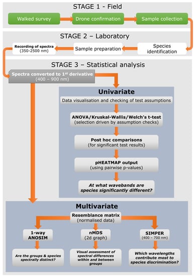
Figure 2.
Overall research flow chart summarizing the methodological processes of the field work, laboratory, and statistical analysis procedures.
Figure 2.
Overall research flow chart summarizing the methodological processes of the field work, laboratory, and statistical analysis procedures.

Figure 3.
Non-metric multidimensional scaling (nMDS) visualizing the variance in spectral reflectance expression: (a) Between species. (b) Between groups.
Figure 3.
Non-metric multidimensional scaling (nMDS) visualizing the variance in spectral reflectance expression: (a) Between species. (b) Between groups.

Figure 4.
Averaged spectral reflectance per species: (a) Raw spectral reflectance. (b) 1st Derivative spectral reflectance.
Figure 4.
Averaged spectral reflectance per species: (a) Raw spectral reflectance. (b) 1st Derivative spectral reflectance.

Figure 5.
Heatmap of pairwise comparison p-values, intra-group comparisons represented by vertical bars. Legend depicting p-values with respect to heat intensity.
Figure 5.
Heatmap of pairwise comparison p-values, intra-group comparisons represented by vertical bars. Legend depicting p-values with respect to heat intensity.

Figure 6.
1-way SIMPER analysis sum percentage contribution to significant dissimilarities made by wavelengths: (a) Between groups. (b) Between species.
Figure 6.
1-way SIMPER analysis sum percentage contribution to significant dissimilarities made by wavelengths: (a) Between groups. (b) Between species.


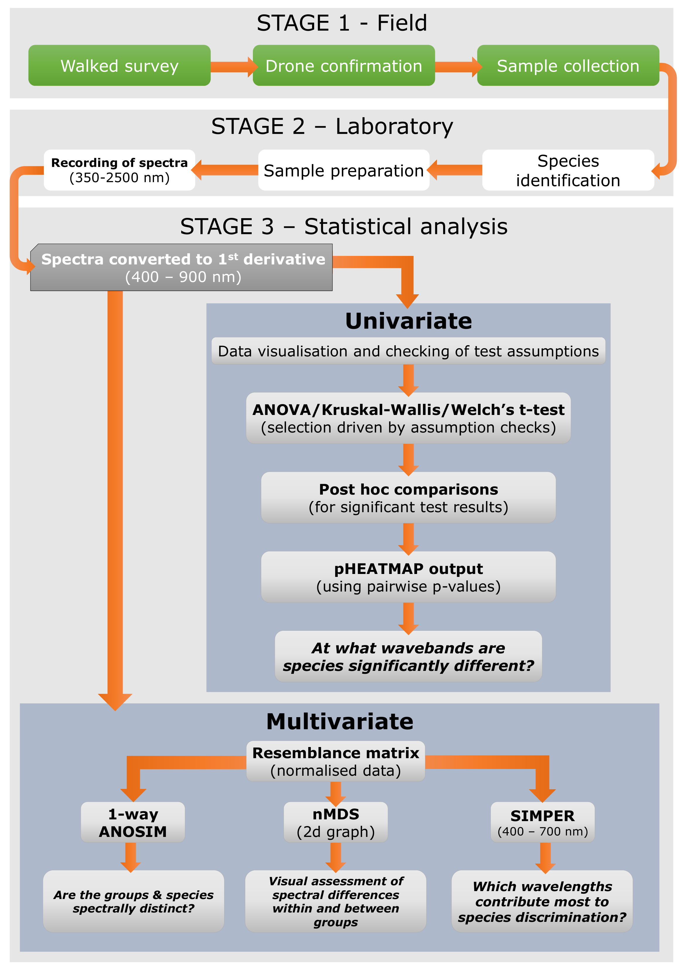
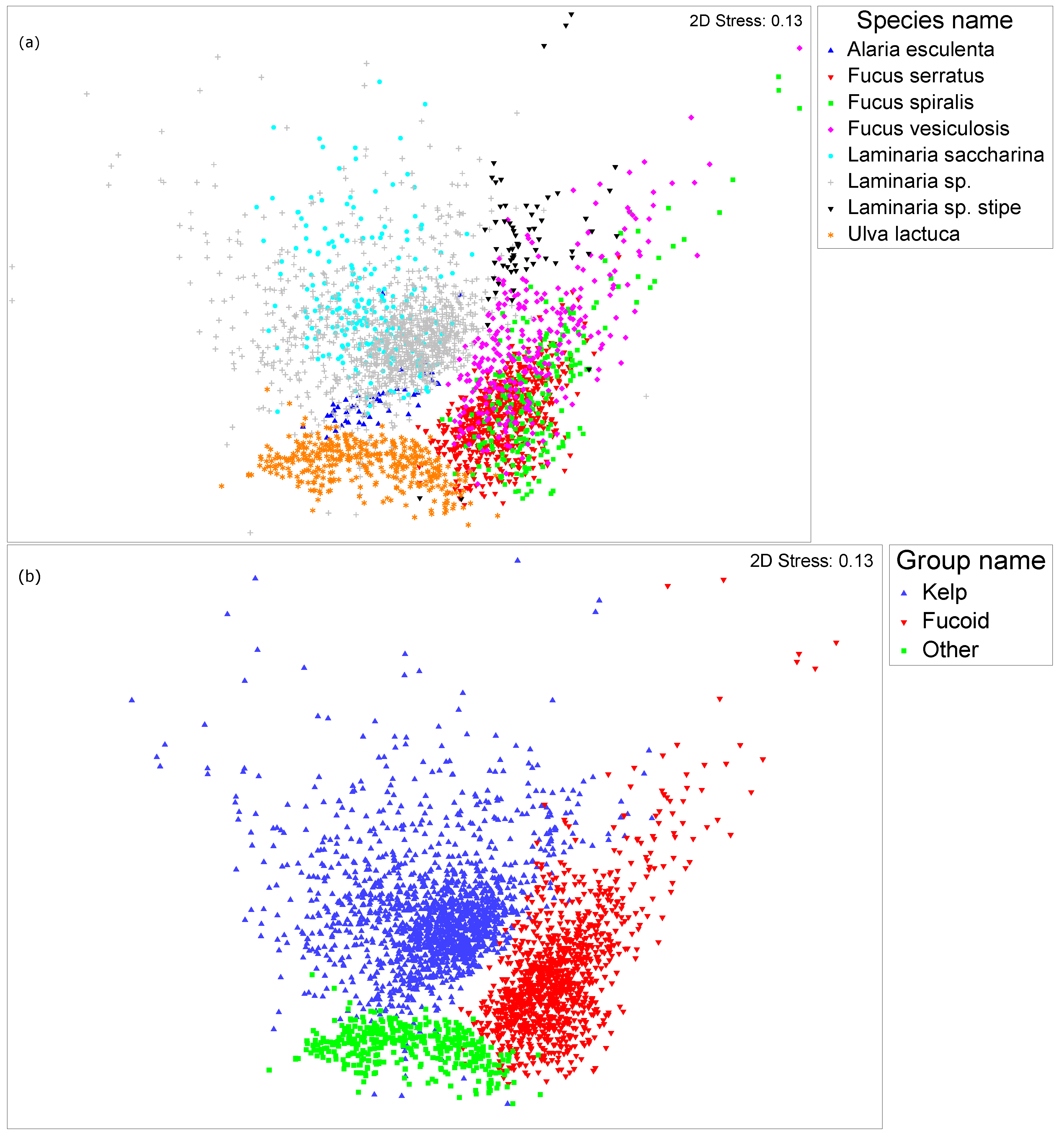
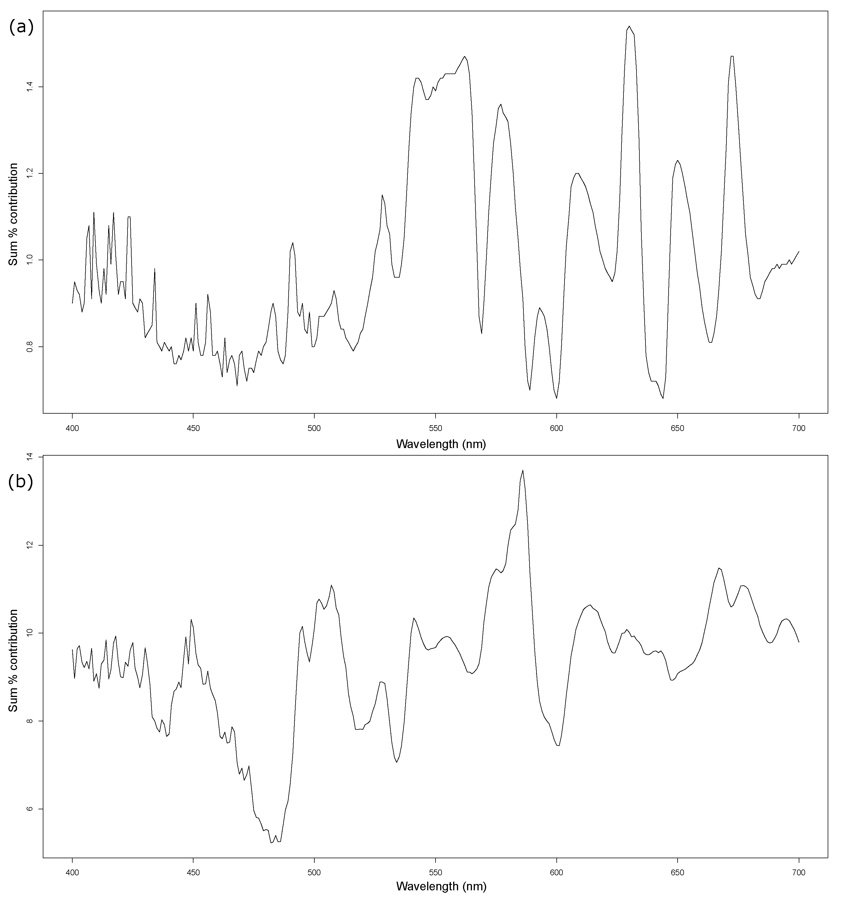
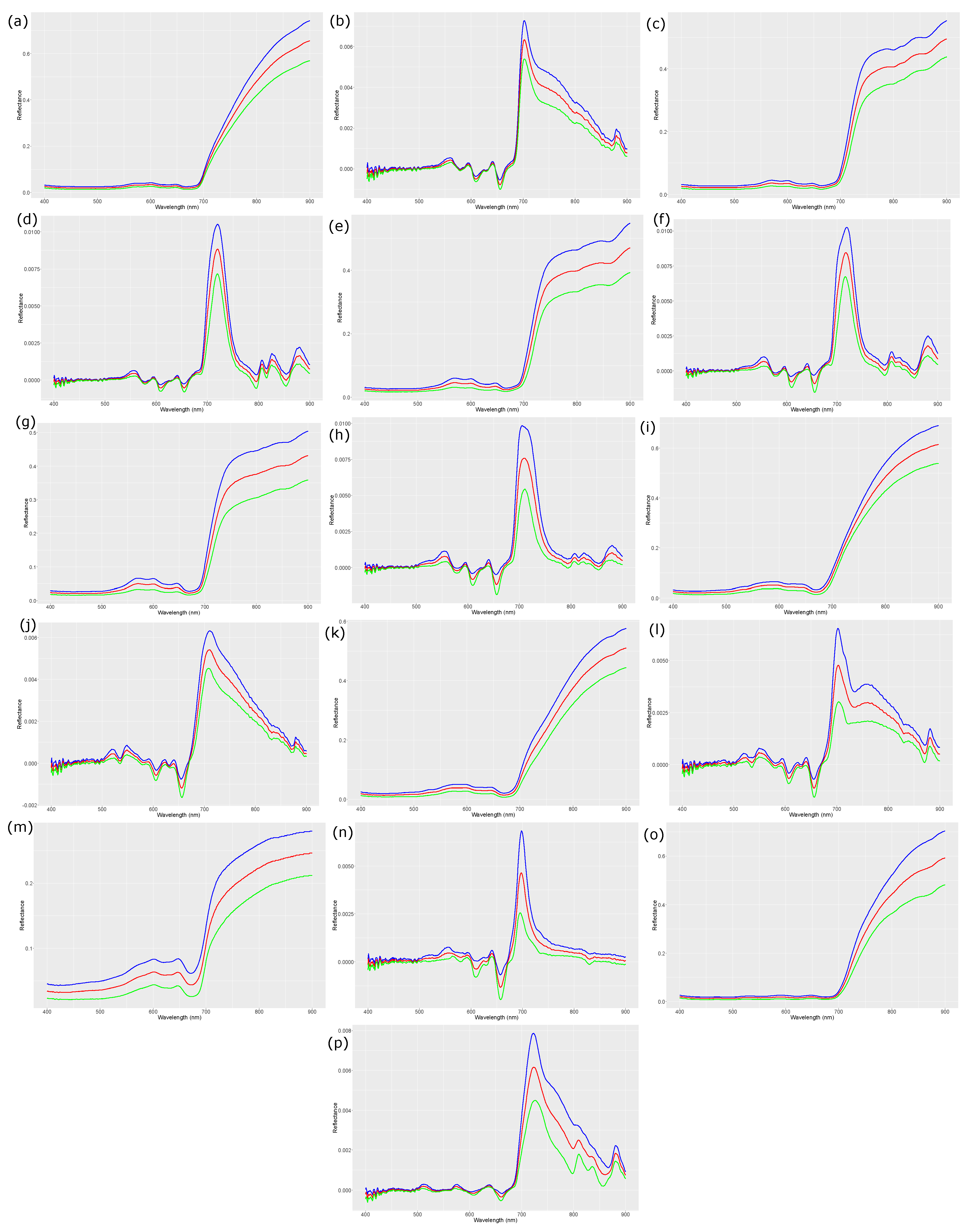
Table 1.
Groups of investigated species causing similar functional damage, the number of readings (n) are displayed in brackets next to each corresponding species.
Table 1.
Groups of investigated species causing similar functional damage, the number of readings (n) are displayed in brackets next to each corresponding species.
| Kelp | Fucoids | Other |
|---|---|---|
| Laminaria saccharina (n = 230) | Fucus vesiculosus (n = 290) | Ulva lactuca (n = 381) |
| Laminaria sp. (n = 1177) | Fucus serratus (n = 612) | |
| Laminaria sp. stipe (n = 68) | Fucus spiralis (n = 228) | |
| Alaria esculenta (n = 47) |
Table 2.
ANOSIM group pairwise R values. All p-values < 0.001. All permutation values = 999.
| Kelp | Fucoid | Other | |
|---|---|---|---|
| Kelp | - | - | - |
| Fucoid | 0.539 | - | - |
| Other | 0.455 | 0.712 | - |
Table 3.
ANOSIM group pairwise R values. All p-values < 0.001. All permutation values = 999. Red cells highlight R > 0.66, amber cells highlight 0.67 > R > 0.33, green cells highlight 0.34 > R. All p-values ≤ 0.001 unless otherwise stated in brackets.
Table 3.
ANOSIM group pairwise R values. All p-values < 0.001. All permutation values = 999. Red cells highlight R > 0.66, amber cells highlight 0.67 > R > 0.33, green cells highlight 0.34 > R. All p-values ≤ 0.001 unless otherwise stated in brackets.
| Alaria esculenta | Fucus serratus | Fucus spiralis | Fucus vesiculosus | Laminaria saccharina | Laminaria sp. | Laminaria sp. stipe | Ulva lactuca | |
|---|---|---|---|---|---|---|---|---|
| Alaria esculenta | - | - | - | - | - | - | - | - |
| Fucus serratus | 0.885 | - | - | - | - | - | - | - |
| Fucus spiralis | 0.750 | 0.331 | - | - | - | - | - | - |
| Fucus vesiculosis | 0.631 | 0.457 | 0.140 | - | - | - | - | - |
| Laminaria saccharina | 0.451 | 0.930 | 0.824 | 0.707 | - | - | - | - |
| Laminariasp. | 0.0617 (0.092) | 0.583 | 0.610 | 0.492 | 0.159 | - | - | - |
| Laminariasp. stipe | 0.795 | 0.969 | 0.786 | 0.559 | 0.872 | 0.685 | - | - |
| Ulva lactuca | 0.490 | 0.848 | 0.830 | 0.805 | 0.797 | 0.533 | 0.939 | - |
© 2019 by the authors. Licensee MDPI, Basel, Switzerland. This article is an open access article distributed under the terms and conditions of the Creative Commons Attribution (CC BY) license (http://creativecommons.org/licenses/by/4.0/).
Share and Cite
MDPI and ACS Style
Mcilwaine, B.; Casado, M.R.; Leinster, P. Using 1st Derivative Reflectance Signatures within a Remote Sensing Framework to Identify Macroalgae in Marine Environments. Remote Sens. 2019, 11, 704. https://doi.org/10.3390/rs11060704
AMA Style
Mcilwaine B, Casado MR, Leinster P. Using 1st Derivative Reflectance Signatures within a Remote Sensing Framework to Identify Macroalgae in Marine Environments. Remote Sensing. 2019; 11(6):704. https://doi.org/10.3390/rs11060704
Chicago/Turabian StyleMcilwaine, Ben, Monica Rivas Casado, and Paul Leinster. 2019. "Using 1st Derivative Reflectance Signatures within a Remote Sensing Framework to Identify Macroalgae in Marine Environments" Remote Sensing 11, no. 6: 704. https://doi.org/10.3390/rs11060704
Note that from the first issue of 2016, this journal uses article numbers instead of page numbers. See further details here.