Decision Fusion Framework for Hyperspectral Image Classification Based on Markov and Conditional Random Fields

Abstract

Classification of hyperspectral images is a challenging task owing to the high dimensionality of the data, limited ground truth data, collinearity of the spectra and the presence of mixed pixels. Conventional classification techniques do not cope well with these problems. Thus, in addition to the spectral information, features were developed for a more complete description of the pixels, e.g., containing contextual information at the superpixel level or mixed pixel information at the subpixel level. This has encouraged an evolution of fusion techniques which use these myriad of multiple feature sets and decisions from individual classifiers to be employed in a joint manner. In this work, we present a flexible decision fusion framework addressing these issues. In a first step, we propose to use sparse fractional abundances as decision source, complementary to class probabilities obtained from a supervised classifier. This specific selection of complementary decision sources enables the description of a pixel in a more complete way, and is expected to mitigate the effects of small training samples sizes. Secondly, we propose to apply a fusion scheme, based on the probabilistic graphical Markov Random Field (MRF) and Conditional Random Field (CRF) models, which inherently employ spatial information into the fusion process. To strengthen the decision fusion process, consistency links across the different decision sources are incorporated to encourage agreement between their decisions. The proposed framework offers flexibility such that it can be extended with additional decision sources in a straightforward way. Experimental results conducted on two real hyperspectral images show superiority over several other approaches in terms of classification performance when very limited training data is available.

1. Introduction

In recent years, hyperspectral image classification has become a very attractive area of research due to the rich spectral information contained in hyperspectral images (HSI). However, in remote sensing, acquiring ground truth information is a difficult and expensive procedure, generally leading to a limited amount of training data. Together with the high number of spectral bands, this results in the Hughes phenomenon [1], which makes HSI classification a challenging task. Moreover, the high spectral similarity between some materials poses additional difficulties, produces ambiguity and further increases the complexity of the classification problem. Moreover, the relatively low spatial resolution of HSI leads to large amounts of mixed pixels, which additionally hinders the classification task.

To tackle these problems, a more complete description of a pixel and its local context has been pursued. Many spatial-spectral methods were developed that include spatial information through contextual features, e.g., by applying morphological and attribute filters, such as extended morphological profiles [2], extended multi-attribute morphological profiles and extended attribute profiles [3,4,5,6,7,8].

In general, spatial-spectral methods employ feature vectors of much higher dimensionality compared to spectral only methods, thereby decreasing the generalization capability of the classifiers for the same amount of training data. To deal with this, feature fusion and decision fusion methods have been developed. In feature fusion, the features are fused directly, for instance in a stacked architecture or using composite or multiple kernels. In [9], a feature fusion method was introduced by using a stacked feature architecture of morphological information and original hyperspectral data. Ref. [10] used different bands and different morphological filters as spatial features to build dedicated kernels and subsequently a composite kernel was built from these individual kernels. Similar composite kernel methods were applied in [11].

Decision fusion methods obtain probability values (decisions) from different individual feature sets by employing probabilistic classifiers and then perform fusion of the decisions. Several papers applied decision fusion rules to combine pixel-based classification results. In [12,13], the majority voting rule was used as a means to fuse several outputs (decisions) produced by basic classifiers. Ref. [14] used consensus theory [15] to generate opinion pool fusion rules to fuse posterior class probabilities obtained from minimum distance classifiers. In [16], probability outputs produced by maximum likelihood classifiers were fused using a weighted linear opinion rule and a weighted majority voting rule. The latter decision fusion rule was also employed for combining the results from supervised SVMs and unsupervised K-means classifiers [17].

Another group of methods applied probabilistic graphical Markov Random Field (MRF) and Conditional Random Field (CRF) models as regularizers after decision fusion. These models perform a maximum a posteriori classification by minimizing an energy function that includes smoothness constraints between neighboring variables. In [18], an MRF regularizer was applied to a linear combination of pixel-based probabilities and superpixel probabilities. In [19], global and local probabilities produced by SVM and subspace multinomial logistic regression classifiers were combined with the linear opinion pool rule and then refined with an MRF regularizer. In a similar manner, in [20], probabilities from probabilistic (one vs. one) SVM and Multinomial Logistic Regression (MLR) classifiers were combined. In [21], rotation forests were used to produce a set of probabilities, which were then fused by averaging over all probability values from the different rotation forests, and regularized by a MRF. In [22], multiple spatial features were used in a fusion framework in which a distinction was made between reliable and unreliable outputs. MRF was then applied to determine the labels of the unreliable pixels. In [23], a method was proposed that linearly combined different decisions, weighted by the accuracies of each of the sources. The obtained single source was then regularized by an MRF.

Apart from being used for spatial regularization, MRFs and CRFs can be used directly as decision fusion methods, by combining multiple sources in their energy function. This strategy has been applied for multisource data fusion in remote sensing [24,25,26,27]. A particularly interesting decision fusion method is proposed in [28] for the fusion of multispectral and Lidar data. They used a CRF model with cross link edges between different feature sources. As far as we know, the strategy of direct decision fusion by using MRF and CRF graphical models has not been applied to the fusion of different decision sources obtained from one hyperspectral image.

In this paper, we propose to perform fusion of different decision sources obtained from one hyperspectral image. The proposed method makes use of MRF and CRF graphical models because of their spatial regularization property and because of their ability to combine multiple decision sources in their energy functions. Since the hyperspectral image is the only image source available, complementary decision sources need to be derived from it. For this, we propose to use fractional abundances, obtained from a sparse unmixing method, SunSAL [29], as decision source. This is expected to provide an improved subpixel description in mixed pixel scenarios and to be well suited in small training size conditions.

Fractional abundances have been applied before, as features for a direct hyperspectral image classification [30], or they were first classified with a soft classifier that generates class probabilities to be used in a decision fusion method [23]. On the other hand, sparse representation classification (SRC) methods were employed. These methods describe a spectrum as a sparse linear combination of training data (endmembers) in a dictionary, similarly as in sparse spectral unmixing. They facilitate the description of mixed pixels and were proven to be well suited for classification of high dimensional data with limited training samples, and in particular for hyperspectral image classification [31]. To employ the spatial correlation of HSI, methods forcing structured sparsity were developed as well [32,33]. To our knowledge, fractional abundances have never been applied directly as decision source in a decision fusion framework.

Along with the abundances, class probabilities from a probabilistic classifier (the MLR classifier) are generated. The input of the MLR classifier is initially provided by the reflectance spectra, but, alternatively, contextual features are applied as input as well. Both decision sources (abundances and probabilities) are two complementary views of the hyperspectral image from a different nature and provide a more complete description of each pixel, which is expected to be favorable in the case of small training sizes. To combine both decision sources, we employ a similar decision fusion approach as the one proposed in [28]. For this, we will use MRF or alternatively CRF graphical models that include, apart from spatial consistency constraints, cross links between the two decision sources to enforce consistency across their decisions. Finally, the framework is extended to accomodate three or more decision sources.

In the experimental section, the proposed strategy is demonstrated to improve over the use of each of the decision sources separately, and over the use of several other feature and decision fusion methods from the literature, in small training size scenarios.

The paper is organized as follows: in Section 2, the key elements of the proposed method are presented. In Section 2.2, the decision sources are introduced, while Section 2.3 and Section 2.4 describe the proposed decision fusion methods MRFL and CRFL. In Section 3, the proposed framework is validated on two real hyperspectral images and compared with several state-of-the-art decision fusion methods. Ultimately, the conclusions are drawn in Section 4.

2. Methodology

2.1. Preliminaries

In this section, we detail our proposed decision fusion approach to combine complementary decision sources based on MRF and CRF graphical models.

2.1.1. MRF Regularization

In the classical single source MRF approach, a graph is defined over a set of n observed pixels $\mathbf{x}=\{{\mathbf{x}}_1,\dots ,{\mathbf{x}}_n\}$ and their corresponding class labels $\mathbf{y}=\{y_1,\dots ,y_n\}$, associated with the nodes in the graph. The graph edges model the spatial neighborhood dependencies between the pixels. While the pixel values are known, the labels are the variables that have to be estimated. In order to accomplish this, the joint probability distribution of the observed data and the labels $P(\mathbf{x},\mathbf{y})$ need to be maximized over $\mathbf{y}$. In terms of energies, the optimal labels are inferred by minimizing the following energy function:

$$E(\mathbf{y})=\sum _{i=1}^n{\psi }_i(y_i)+\beta \sum _{i=1}^n\sum _{j\in {\mathbf{N}}_{\mathbf{i}}}{\psi }_{i,j}(y_i,y_j),$$

(1)

where ${\psi }_i(y_i)=-ln(p({\mathbf{x}}_i|y_i))$ are the unary potentials, obtained from the class conditional probabilities $p({\mathbf{x}}_i|y_i)$ [34]. For high dimensional data, one resorts to the more commonly used: ${\psi }_i(y_i)=-ln(\widehat{p}(y_i|{\mathbf{x}}_i)),$ where $\widehat{p}(y_i|{\mathbf{x}}_i)$ are the estimated posterior probabilities, obtained from a probabilistic classifier [15,35]. The values $\widehat{p}(y_i|{\mathbf{x}}_i)$ are calculated by using the spectral reflectance values of the HSI pixels as features, but, in general, other (e.g., contextual) features may be applied as the inputs to the probabilistic classifier to obtain the posterior probabilities.

${\psi }_{i,j}=(1-\delta (y_i,y_j))$ are the pairwise potentials which are only label dependent and impose smoothness, based on the similarity of the labels within the spatial neighborhood ${\mathbf{N}}_{\mathbf{i}}$ of pixel i. In the above, $\delta (y_i,y_j)$ denotes the indicator function ($\delta (a,b)=1$ for $a=b$ and $\delta (a,b)=0$, otherwise).

2.1.2. CRF Regularization

One of the drawbacks of the MRF method is that it models the neighborhood relations between the labels without taking the observed data into account. It is a generative model, estimating the joint distribution of the data and the labels. Conditional Random Fields have several desirable properties, making them more flexible and efficient: (1) They are discriminative models, estimating $P(\mathbf{y}|\mathbf{x})$ directly, (2) They take into account the observed data in their pairwise potential terms, i.e., they impose smoothness based on the similarity of the observations within the spatial neighborhood of the pixels.

2.2. The Decision Sources

Let $\mathbf{x}=\{{\mathbf{x}}_1,\dots ,{\mathbf{x}}_n\}$ be a hyperspectral image containing n pixels, with ${\mathbf{x}}_i\in R^d$, d being the number of spectral bands. $D=\left\{({\mathbf{x}}_1,y_1)\right\},\dots ,({\mathbf{x}}_m,y_m)\}$ is a training set containing $j=1,\dots ,m$ labeled samples ${\mathbf{x}}_j$ and their associated labels $y_j\in \{1,\dots ,C\},$ where C is the number of classes. The aim is to assign labels $y_i$ to each image pixel ${\mathbf{x}}_i$.

In this work, the MRFs and CRFs are used as decision fusion methods, by combining multiple decision sources in their energy functions. We propose the fusion of two decision sources. The first is the probability output from the Multinomial Logistic Regression classifier (MLR) [36], i.e., a supervised classification of the spectral reflectance values. The second source of information is produced by considering the sparse spectral unmixing method SunSAL proposed in [29].

As a first source of information, the spectral values of the pixels are employed as input to an MLR, to obtain classification probabilities for each pixel ${\mathbf{x}}_i$: ${\mathbf{p}}_i=\mathbf{p}({\mathbf{x}}_i)=(p_1({\mathbf{x}}_i),\dots ,p_C({\mathbf{x}}_i))$, with:

$$p_c({\mathbf{x}}_i)=p(y_i=c|{\mathbf{x}}_i)=\frac{exp({\mathit{\beta }}_c^T{\mathbf{x}}_{\mathbf{i}})}{{\sum }_{c=1}^{C}exp({\mathit{\beta }}_c^T{\mathbf{x}}_{\mathbf{i}})},$$

(2)

where ${\mathit{\beta }}_c\in R^d$, ($c=1,\dots ,C$) are the regression coefficients, estimated from the training data. A class label can be estimated from the probability vector, e.g., by applying a Maximum a Posteriori (MAP) classifier to it: ${\widehat{y}}_i^p=arg{max}_c{p}_c({\mathbf{x}}_i)$.

The second source of information is obtained by computing the fractional abundances of each pixel ${\mathbf{x}}_i$ with SunSAL, in which the training data is used as a dictionary of endmembers, $\mathit{E}=[{\mathbf{x}}_1,\dots ,{\mathbf{x}}_m]$ (i.e., the training pixels are assumed to be pure materials):

$$\begin{array}{ccc}\hfill {\mathit{\alpha }}^{*}& =& ({\alpha }_1^{*},\dots ,{\alpha }_m^{*})\hfill \\ & =& arg\underset{\alpha }{min}\frac{1}{2}\parallel \mathbf{E}\mathit{\alpha }-{\mathbf{x}}_{\mathbf{i}}{\parallel }_2^2+\lambda {\parallel \mathit{\alpha }\parallel }_1,\hfill \\ & & \mathrm{s}.\mathrm{t}.\mathit{\alpha }\ge 0.\hfill \end{array}$$

(3)

Then, the obtained abundances that correspond to endmembers having class label $y_j=c$ are summed up to obtain one fractional abundance ${\alpha }_c({\mathbf{x}}_i)$ per class c, and the abundance vector: ${\mathit{\alpha }}_i=\mathit{\alpha }({\mathbf{x}}_i)=({\alpha }_1({\mathbf{x}}_i),\dots ,{\alpha }_C({\mathbf{x}}_i))$. In a similar way as with the vector of classification probabilities, a class label can be estimated from the abundance vector, e.g., by applying a MAP classifier to it: ${\widehat{y}}_i^{\alpha }=arg{max}_c{\alpha }_c({\mathbf{x}}_i)$, similarly as in the sparse representation classifiers.

Rather than expressing the statistical probability that a pixel is correctly classified as belonging to class c, the abundances express the fractional presence of class c within the pixel. They are expected to contain complementary information to the classification probabilities, in particular in mixed pixel scenarios. The use of both decision sources allows for a more complete description of the pixels, which is favorable for high-dimensional data and small training size conditions.

Once the individual $\mathit{\alpha }$ and $\mathbf{p}$ are obtained from the sparse unmixing and the MLR classifier, the decision fusion of these modalities is performed in terms of MRF and CRF graphical models with composite energy functions, including the contributions from both decision sources.

2.3. MRF with Cross Links for Fusion (MRFL)

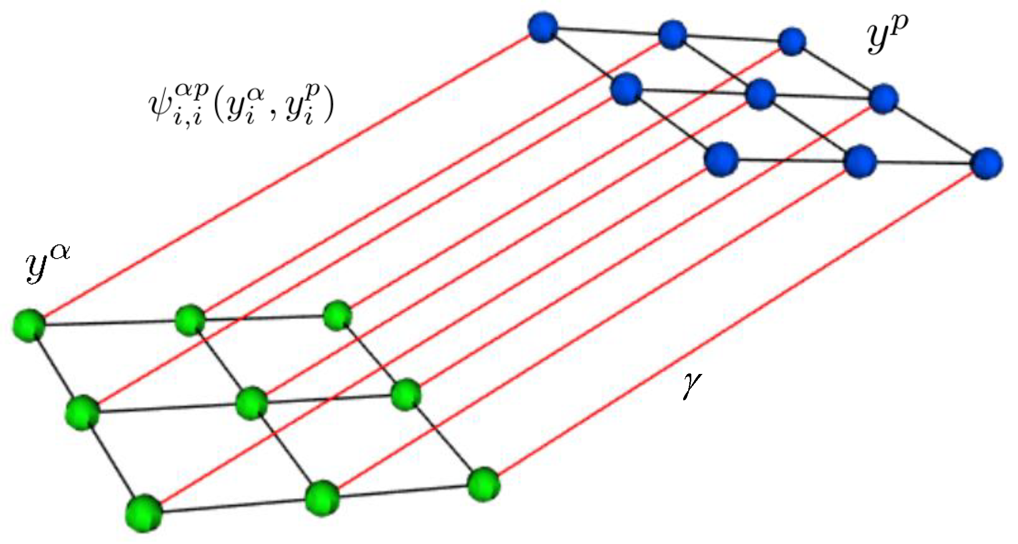
With each decision source, class labels are associated, i.e., $y_i^{\alpha }$ for the sparse abundances and $y_i^p$ for the classification probabilities. To allow both decision sources to be fused, a bipartite graph is considered, containing two types of nodes for each pixel, denoting random variables associated with the labels $y_i^{\alpha }$ and $y_i^p$, respectively. Now, for each type of nodes, edges are defined that model the spatial neighborhood dependencies between the pixels. Moreover, a cross link is defined, connecting both nodes, i.e., connecting label $y_i^{\alpha }$ with the corresponding label $y_i^p$ [37] (see Figure 1). Adding this cross link encourages the estimates ${\widehat{y}}_i^{\alpha }$ and ${\widehat{y}}_i^p$ to be the same, i.e., promotes consistency between both decisions. Remark that other cross links are possible (e.g., between neighboring pixels), which were omitted here to avoid possible performance degradation in the case of a denser graph.

The goal is now to optimize the joint distribution over the observed data and corresponding labels from both sources: $P(\mathit{\alpha },\mathit{p},{\mathbf{y}}^{\alpha },{\mathbf{y}}^p)$. For this, the following energy function is minimized:

$$\begin{array}{c}\hfill E({\mathbf{y}}^{\alpha },{\mathbf{y}}^p)=\sum _{i=1}^n{\psi }_i^{\alpha }(y_i^{\alpha })+\sum _{i=1}^n{\psi }_i^p(y_i^p)\\ \hfill +\beta \left[\sum _{i=1}^n\sum _{j\in {\mathbf{N}}_{\mathbf{i}}}{\psi }_{i,j}^{\alpha }(y_i^{\alpha },y_j^{\alpha })+\sum _{i=1}^n\sum _{j\in {\mathbf{N}}_{\mathbf{i}}}{\psi }_{i,j}^p(y_i^p,y_j^p)\right]\\ \hfill +\gamma \sum _{i=1}^n{\psi }_{i,i}^{\alpha p}(y_i^{\alpha },y_i^p).\end{array}$$

(4)

The unary potentials are given by: ${\psi }_i^{\alpha }(y_i^{\alpha })=-ln({\alpha }_c({\mathbf{x}}_i))$ and ${\psi }_i^p(y_i^p)=-ln(p_c({\mathbf{x}}_i))$ with $y_i=c$. ${\mathbf{N}}_{\mathbf{i}}$ is a 4-spatial neighborhood. The pairwise potentials from the individual sources: ${\psi }_{i,j}^{\alpha }=(1-\delta (y_i^{\alpha },y_j^{\alpha }))$ and ${\psi }_{i,j}^p=(1-\delta (y_i^p,y_j^p))$ impose smoothness based on the similarity of the labels within the spatial neighborhood of pixel i, obtained from the fractional abundances and the classification probabilities, respectively. The last pairwise term ${\psi }_{i,i}^{\alpha p}=(1-\delta (y_i^{\alpha },y_i^p))$ penalizes disagreement between the labels $y_i^{\alpha }$ and $y_i^p$. Through the binary potentials, the MRFL accounts simultaneously for spatial structuring and consistency between the labelings from the two decision sources.

The minimization of this energy function is an NP-hard combinatorial optimization problem. Nevertheless, there exist methods which can solve this problem efficiently in an approximate way. We have applied the graph-cut $\alpha$-expansion algorithm [38,39,40,41]. Since the last term ${\psi }_{i,i}^{\alpha p}$ encourages cross-source label consistency, for the vast majority of the pixels, one can expect an equivalent estimation of the labels ${\widehat{y}}_i^{\alpha }$ = ${\widehat{y}}_i^p$. For this reason, any of the two may be used as the final labeling result. We refer to [28] for more details on the probabilistic framework for graphical models with such cross-links.

2.4. CRF with Cross Links for Fusion (CRFL)

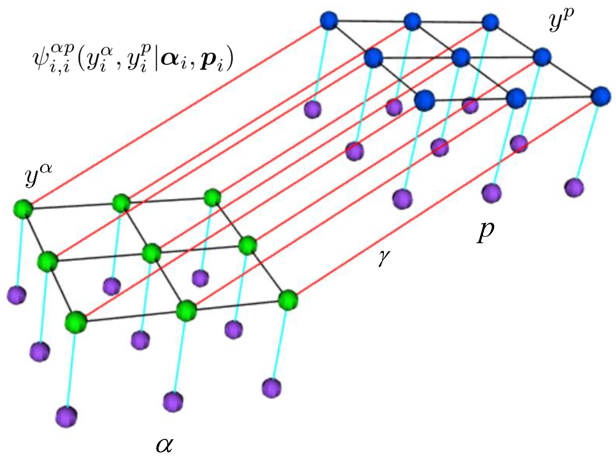
The above method is a generative model and models the joint probability distribution of the labels and the observed data: $P(\mathit{\alpha },\mathit{p},{\mathbf{y}}^{\alpha },{\mathbf{y}}^p)$. Moreover, only relationships between the class labels are taken into account in the pairwise potentials of the MRFL. As an alternative, we employ a discriminative method which is a generalization of the previous MRFL method, directly modeling the posterior distribution $P({\mathbf{y}}^{\alpha },{\mathbf{y}}^p|\mathit{\alpha },\mathit{p})$, by simultaneously taking into account both the relationships between the class labels $y^{\alpha }$, $y^p$ and the observed data: α, p in the pairwise potentials (see Figure 2).

We refer the reader to [27,28,37].

The energy function is now given by:

$$\begin{array}{c}E({\mathbf{y}}^{\alpha },{\mathbf{y}}^p|\mathit{\alpha },\mathit{p})=\sum _{i=1}^n{\psi }_i^{\alpha }(y_i^{\alpha })+\sum _{i=1}^n{\psi }_i^p(y_i^p)\\ +\beta \left[\sum _{i=1}^n\sum _{j\in {\mathbf{N}}_{\mathbf{i}}}{\psi }_{i,j}^{\alpha }(y_i^{\alpha },y_j^{\alpha }|{\mathit{\alpha }}_i,{\mathit{\alpha }}_j)+\sum _{i=1}^n\sum _{j\in {\mathbf{N}}_{\mathbf{i}}}{\psi }_{i,j}^p(y_i^p,y_j^p|{\mathit{p}}_i,{\mathit{p}}_j)\right]\\ +\gamma \sum _{i=1}^n{\psi }_{i,i}^{\alpha p}(y_i^{\alpha },y_i^p|{\mathit{\alpha }}_i,{\mathit{p}}_i).\end{array}$$

(5)

The unary terms are equivalent to the ones in the MRFL model. For the pairwise potentials, a contrast sensitive Potts model is applied [42]:

• ${\psi }_{i,j}^{\alpha }(y_i^{\alpha },y_j^{\alpha }|{\mathit{\alpha }}_i,{\mathit{\alpha }}_j)=(1-\delta (y_i^{\alpha },y_j^{\alpha }))exp(-\frac{{\parallel \mathit{\alpha }}_i-{\mathit{\alpha }}_j{\parallel }_2^2}{{\sigma }^{\alpha }}),$
• ${\psi }_{i,j}^p(y_i^p,y_j^p|{\mathit{p}}_i,{\mathit{p}}_j)=(1-\delta (y_i^p,y_j^p))exp(-\frac{{\parallel \mathit{p}}_i-{\mathit{p}}_j{\parallel }_2^2}{{\sigma }^p}),$
• ${\psi }_{i,i}^{\alpha p}(y_i^{\alpha },y_i^p|{\mathit{\alpha }}_i,{\mathit{p}}_i)=(1-\delta (y_i^{\alpha },y_i^p))exp(-\frac{{\parallel \mathit{\alpha }}_i-{\mathit{p}}_i{\parallel }_2^2}{{\sigma }^{\alpha p}}).$

The first term encourages neighboring pixels with similar abundance vectors to belong to the same class. The second term encourages neighboring pixels with similar class probabilities to belong to the same class. Finally, the third term encourages to assign similar class labels $y_i^{\alpha }$ and $y_i^p$ to pixels for which the abundance vector is similar to the probability vector. The parameters $\sigma$ are standard deviations that determine the strengths of these enforcements. The optimization of this energy function is again performed with the graph-cut $\alpha$-expansion algorithm.

Our proposed methods use the graph-cut $\alpha$-expansion algorithm [38,39,40,41], which has a worst case complexity of $\mathcal{O}(m{n}^2|P|)$ for a single optimization problem where m denotes the number of edges, n denotes the number of nodes in the graph and |P| denotes the cost of the minimum cut. Thus, the theoretical computational complexity of our proposed method is: $\mathcal{O}(kCm{n}^2|P|)$, with k the upper bound of the number of iterations and C the number of classes. With a non-cautious addition of edges in the graph, for instance adding a cross link between each node and all other nodes from the second source, there would be a quadratic increase in the computational complexity. On the other hand, the empirical complexity in real scenarios has been shown to be between linear and quadratic w.r.t. the graph size [38].

3. Experimental Results and Discussion

3.1. Hyperspectral Data Sets

We validated our method on two well-known hyperspectral images: the “ROSIS-03 University of Pavia” and the “AVIRIS Indian Pines” images.

3.1.1. University of Pavia

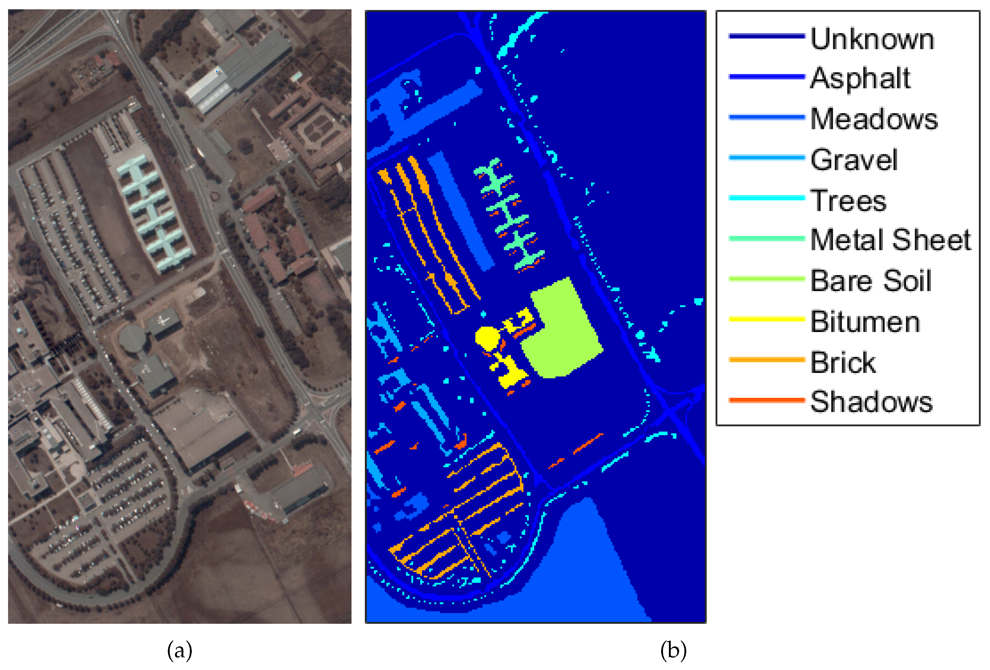
This scene was acquired by the ROSIS-03 sensor over the University of Pavia, Italy. It contains 610 × 340 pixels, with a spatial resolution of 1.3 m per pixel, and 115 bands with a spectral range from 0.43 to 0.86 $\mathsf{\mu }$m. Twelve noisy bands have been removed, and the remaining 103 spectral channels are used. A false color composite image along with the available ground reference map is shown in Figure 3.

3.1.2. Indian Pines

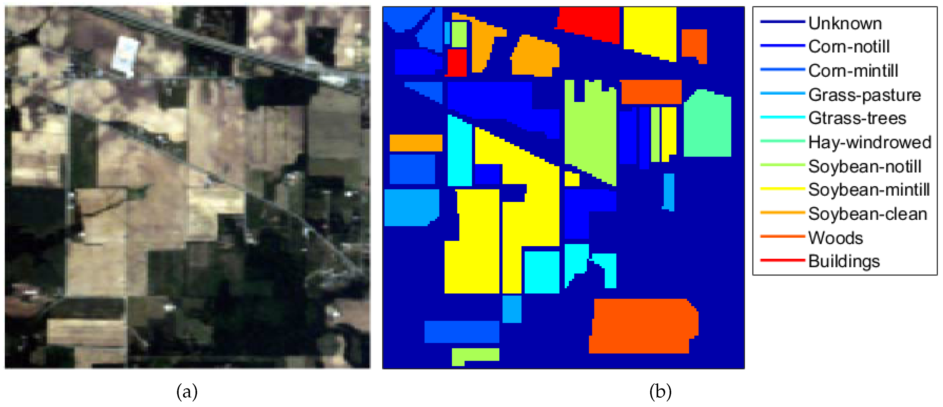
Indian Pines was acquired by the AVIRIS sensor over an agricultural site in Northwestern Indiana. This scene consists of 145 × 145 pixels with a spatial resolution of 20 m and 220 spectral bands, ranging from 0.2 to 2.3 $\mathsf{\mu }$m. Prior to using the dataset, the noisy bands and the water absorption bands were manually discarded, leaving us with 164 bands. An RGB image of the scene along with the available ground reference map is shown in Figure 4.

3.2. Parameter Settings

In the experiments, we validated the following specific aspects of the proposed methodology:

• the performance of the sparse representation obtained by the pixels fractional abundances from SunSAL as decisions, when combined with classification probabilities in a decision fusion scheme;
• the comparison of the performances of MRFL and CRFL as decision fusion methods;
• the flexibility of the proposed fusion methods, by including additional decision sets;
• the performance of the method in the case of small training sample sizes.

The parameters which are part of the proposed methods were set as follows: to generate a balanced small training set, we randomly selected 10 pixels per class from both datasets. This training set was used to estimate the regression coefficients of the MLR classifier and to form the endmember dictionary of the sparse unmixing method.

For both datasets, the regularization parameter from the unmixing method was empirically selected from the range: $\lambda \in$ [10${}^{-5}$–0.5] using a grid search method and the abundances were normalized. The inference parameters $\beta$, controlling the influence of the spatial neighborhood and $\gamma$, controlling the influence of the cross link consistency were set by a grid search in the range: [0.1–25]. The parameters ${\sigma }_{\alpha },{\sigma }_p,{\sigma }_{\alpha p}$ from the pairwise potentials of the CRFL method were determined as the mean squared differences between the abundances, between the probabilities and the mean squared differences between the abundances and probabilities, respectively [43]. The obtained optimal values for $\lambda$, $\beta$ and $\gamma$ are summarized in

Table 1. Optimal values of the parameters.

Image	$\mathit{\lambda }$	${\mathit{\beta }}_{\mathit{MRFL}}$	${\mathit{\gamma }}_{\mathit{MRFL}}$	${\mathit{\beta }}_{\mathit{CRFL}}$	${\mathit{\gamma }}_{\mathit{CRFL}}$
University of Pavia	$5\times {10}^{-4}$	1.0	1.0	25	25
Indian Pines	${10}^{-3}$	1.0	0.8	5	25

.

Remark that $\beta$ represents the total weight of all neighborhood pairwise interactions for both modalities in Equations (4) and (5). In a 4-connected neighborhood, all pairwise interactions are weighted equally with $\frac{\beta }{8}$.

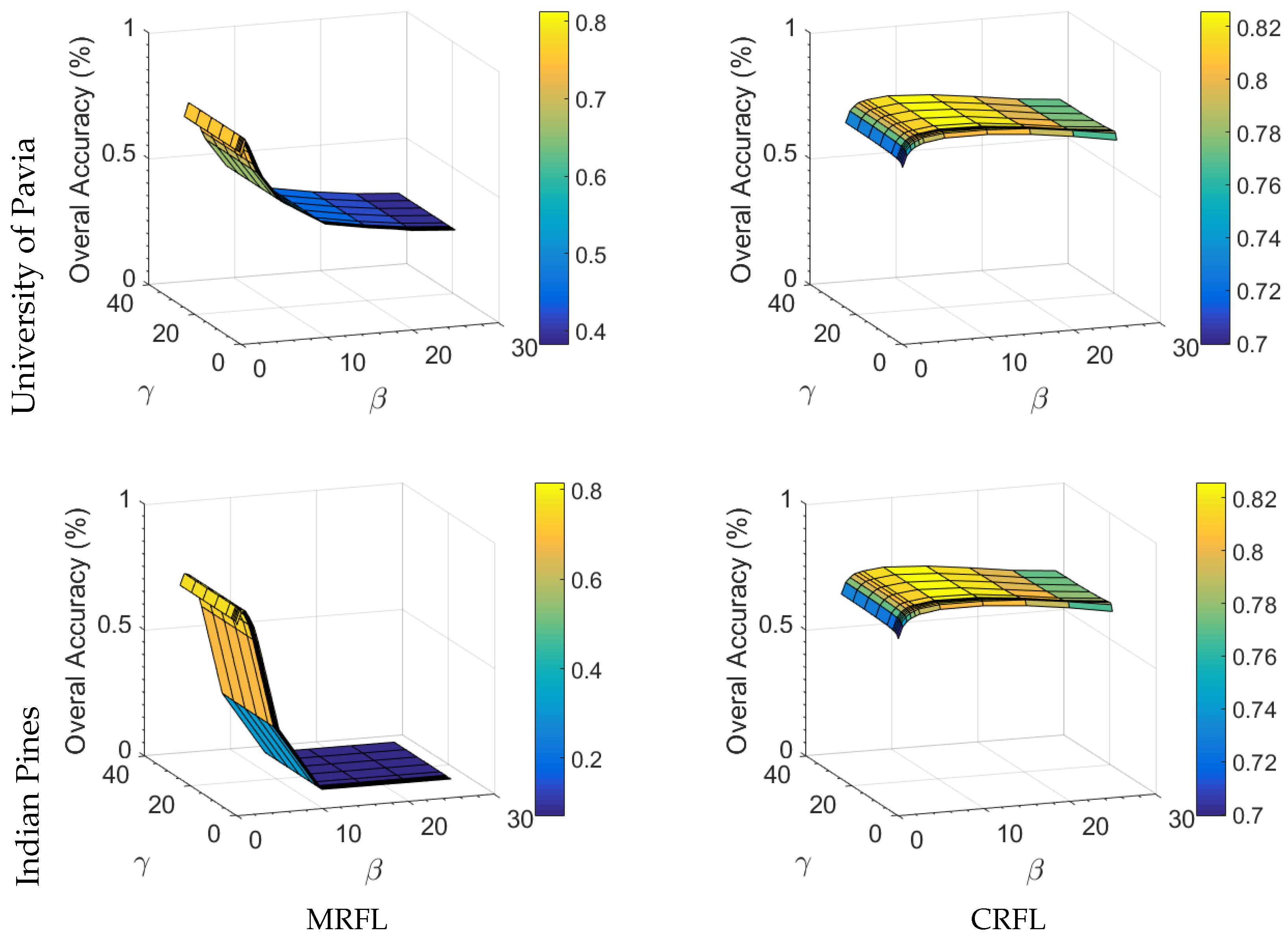
Optimal values of $\lambda$ are small, an observation reported in other work as well [44,45]. Accuracies remained stable for values of $\lambda$ in the range $\lambda \in$ [10${}^{-3}$–10${}^{-5}$]. We performed a sensitivity analysis of the inference parameters $\beta$ and $\gamma$ of our MRFL and CRFL decision fusion methods. Figure 5 shows the evolution of the Overal Accuracy (OA) as a function of the inference parameters. In what follows, we discuss the results from the table and the figure. The following conclusions can be drawn:

• The OA initially improves with increasing $\beta$ and $\gamma$, proving the effectiveness of incorporating the spatial neighborhood and the consistency terms in our proposed methods, to correct for the wrongly initially assigned labels from the individual sources.
• In general, the OA is more sensitive to changes of $\beta$, and remains relatively stable for a large range of values of $\gamma$.
• A significant accuracy drop can be observed for higher values of $\beta$ and $\gamma$ in the MRFL method, whereas the CRFL method produces more stable results for different combinations of $\beta$ and $\gamma$. This allows for applying the CRFL method to other images without having to perform extensive and exhaustive parameter grid searches.
• The optimal values of $\beta$ and $\gamma$ are substantially higher for CRFL than for MRFL. This is because the CRFL method inherently uses observed data in the pairwise potentials, and thus heavily penalizes small differences between decisions that correspond to different class labels.
• For the Indian Pines image, $\gamma$ is much higher than $\beta$ in the case of CRFL. This can be attributed to the presence of large homogeneous regions that imply a low influence of the spatial neighborhood compared to the consistency terms. In contrast, the University of Pavia image contains less large homogeneous regions, leading to an increase of the influence of the spatial neighborhood, with larger values of $\beta$ in the case of CRFL.

3.3. Experiments

3.3.1. Experiment 1: Complementarity of the Abundances

In this section, we study the potential of the abundances $\mathit{\alpha }({\mathbf{x}}_i)$, obtained by the SunSAL algorithm as decision sources for classification. As a first step, we investigated the complementarity of these sources when compared to the class probabilities $\mathit{p}({\mathbf{x}}_i)$, obtained from the MLR classifier. For this, we apply a MAP classifier to both the abundances, obtaining class labels ${\widehat{y}}_i^{\alpha }=arg{max}_c{\alpha }_c({\mathbf{x}}_i)$, and the MLR class probabilities, obtaining ${\widehat{y}}_i^p=arg{max}_c{p}_c({\mathbf{x}}_i)$. From these, a confusion matrix is generated, in which each element $(k,l)$ shows the percentage of the pixels that was classified as class k by the first and as class l by the second classifier. The obtained confusion matrices for the University of Pavia and Indian Pines images are shown in Figure 6. To compare, the confusion matrices between the MLR classifier and a SVM classifier are given as well.

One can clearly notice that there is a higher spread in the confusion matrices of SunSAL versus MLR than in the ones of SVM versus MLR. This indicates that SunSAL and MLR disagree more than MLR and SVM do, and that the abundances provide more complementary information to the MLR probabilities than the SVM class probabilities do. This makes the abundances a good candidate decision source in a decision fusion approach.

3.3.2. Experiment 2: Validation of the Decision Fusion Framework

Next, we validate the proposed decision fusion methods MRFL and CRFL by comparing them with several other classification and decision fusion methods. For a fair comparison, all comparing methods are applied on the same two decision sets: the abundances and the class probabilities. Some methods only employ one single source while other methods perform a decision fusion of both sources. Some methods are spectral only, i.e., they do not infer information from neighboring pixels, while other are spatial-spectral methods.

The proposed methods MRFL and CRFL are compared to the following methods:

• SunSAL [29]—sparse spectral unmixing is applied to each test pixel, obtaining the abundance vector $\mathit{\alpha }({\mathbf{x}}_i)=({\alpha }_1({\mathbf{x}}_i),\dots ,{\alpha }_C({\mathbf{x}}_i))$. From this vector, the pixel is labeled as the class corresponding to the largest abundance value: ${\widehat{y}}_i^{\alpha }=arg{max}_c{\alpha }_c({\mathbf{x}}_i)$. This is a single source, spectral only method.
• MLR—Multinomial Logistic Regression classifier [36] generating the class probabilities $\mathbf{p}({\mathbf{x}}_i)=(p_1({\mathbf{x}}_i),\dots ,p_C({\mathbf{x}}_i))$. From this vector, the pixel is labeled as the class corresponding to the largest probability ${\widehat{y}}_i^p=arg{max}_c{p}_c({\mathbf{x}}_i)$. This is also a single source, spectral only method.
• LC—linear combination, a simple decision fusion approach, using a linear combination of the obtained abundances and class probabilities by applying the linear opinion pool rule from: [15]. This is a spectral only fusion method. This method was applied in [30] on the same sources as initialisation for a semi-supervised approach.
• MRFG_a [23]—a decision fusion framework from the recent literature. The principle of this method is to linearly combine different decision sources, weighted by the accuracies of each of the sources. The obtained single source is then regularized by a MRF, as in Equation (1). In [23], three different sources were applied. For a fair comparison, we apply their fusion method with the abundances and class probabilities from our method as decision sources.
• MRFG—the same decision fusion method as MRFG_a, but this time, the posterior classification probabilities from the abundances as obtained in [23] are employed. In that work, the abundances were obtained with a matched filtering technique. To produce the posterior classification probabilities, the MLR classifier was used.
• MRF_a—this method applies a MRF regularization on the output of SunSAL as a single source. This is a spatial-spectral single source method.
• MRF_p—a spatial-spectral single source method, applying MRF as a regularizer on the output of the MLR classifier.
• CRF_a—a spatial-spectral single source method, applying CRF as a regularizer on the output of SunSAL.
• CRF_p—a spatial-spectral single source method, applying CRF as a regularizer on the output of the MLR classifier.

For the proposed methods, the parameters $\lambda ,\beta$ and $\gamma$ are set as in Table 1. The parameter $\beta$ from the MRFG and MRFG_a methods are set as in [23], i.e., $\beta =0.5$. For the methods where we use MRF and CRF as regularizers, optimal values of the parameters were obtained by a grid search.

All experiments were run on a PC with Intel i7-6700K and 32 GB RAM. The execution time for one run with fixed parameters was in the order of a second for the MRFL and a minute for the CRFL. When performing grid search and averaging over 100 runs, we run the experiments on the UAntwerpen HPC (CalcUA Super-computing facility) having nodes with 128 GB and 256 GB RAM and 2.4 GHz 14-core Broadwell CPUs, on which the different runs were distributed, leading to speedups with a factor of 10–50.

(a) University of Pavia dataset

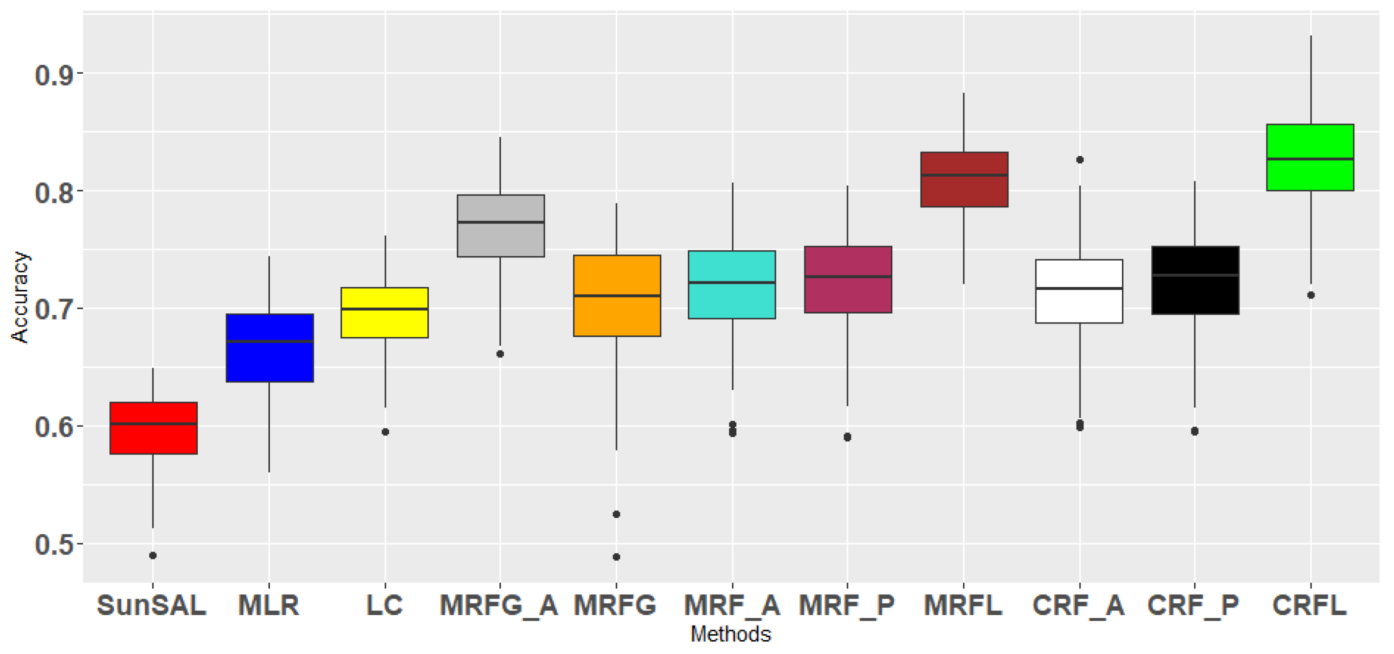
Each of the described methods is applied on the University of Pavia image, with a training set of 10 pixels per class. Experiments are repeated 100 times. In

Table 2. Classification accuracies [%] with their standard deviations for the University of Pavia image (the highest accuracies are denoted in bold).

Class	Train	Test	SunSAL	MLR	LC	MRFG_a	MRFG	MRF_a	MRF_p	MRFL	CRF_a	CRF_p	CRFL
Asphalt	10	6621	33.04 $\pm 9.09$	50.72 $\pm 9.30$	50.42 $\pm 8.98$	66.60 $\pm 12.90$	58.05 $\pm 13.20$	52.26 $\pm 18.50$	58.80 $\pm 11.40$	77.56 $\pm 12.80$	50.40 $\pm 17.60$	59.28 $\pm 11.90$	77.86$\pm 17.80$
Meadows	10	18,639	68.95 $\pm 8.46$	67.16 $\pm 9.91$	73.46 $\pm 7.46$	78.08 $\pm 18.00$	71.18 $\pm 13.60$	80.97 $\pm 11.30$	71.80 $\pm 11.10$	82.13 $\pm 8.30$	81.66 $\pm 10.90$	72.70 $\pm 11.38$	88.74$\pm 8.10$
Gravel	10	2089	60.59 $\pm 9.12$	70.93 $\pm 7.51$	77.01 $\pm 5.54$	87.85 $\pm 7$	71.18 $\pm 13.60$	88.30 $\pm 10.30$	78.82 $\pm 9.40$	90.90 $\pm 7.90$	86.49 $\pm 10.10$	76.86 $\pm 9.20$	92.71$\pm 9.80$
Trees	10	3054	84.61 $\pm 7.38$	88.95 $\pm 5.96$	91.49 $\pm 4.41$	91.79 $\pm 4.70$	91.72 $\pm 5.50$	91.56 $\pm 5.80$	88.92 $\pm 6.20$	91.95$\pm 5.00$	90.80 $\pm 5.80$	88.76 $\pm 6.20$	89.51 $\pm 6.80$
Metal Sheet	10	1335	95.43 $\pm 3.72$	97.81 $\pm 1.53$	98.71 $\pm 0.85$	98.96 $\pm 0.77$	98.85 $\pm 0.75$	99.30 $\pm 1.50$	98.11 $\pm 1.30$	99.46$\pm 0.40$	98.59 $\pm 2.30$	97.88 $\pm 1.47$	99.28 $\pm 1.30$
Bare Soil	10	5019	46.80 $\pm 10.18$	55.85 $\pm 9.02$	56.10 $\pm 8.59$	59.9 $\pm 11.00$	59.90 $\pm 14.60$	53.44 $\pm 18.50$	59.18 $\pm 11.20$	61.29 $\pm 13.60$	52.20 $\pm 18.90$	59.04 $\pm 11.40$	63.07$\pm 27.00$
Bitumen	10	1320	48.80 $\pm 11.87$	80.75 $\pm 8.68$	83.24 $\pm 6.74$	95.43 $\pm 2.70$	87.82 $\pm 12.12$	91.07 $\pm 10.30$	90.98 $\pm 6.90$	97.14$\pm 2.80$	90.15 $\pm 10.00$	89.87 $\pm 7.40$	96.55 $\pm 7.80$
Bricks	10	3672	36.74 $\pm 11.04$	61.60 $\pm 9.37$	55.99 $\pm 8.59$	71.85 $\pm 13.80$	63.11 $\pm 17.00$	34.75 $\pm 23.52$	72.33 $\pm 11.70$	72.64$\pm 17.60$	34.72 $\pm 22.00$	72.64$\pm 11.40$	58.25 $\pm 28.00$
Shadows	10	937	98.61 $\pm 10.11$	95.52 $\pm 2.42$	99.31 $\pm 0.47$	99.83 $\pm 0.16$	99.66 $\pm 0.50$	99.96 $\pm 0.09$	96.88 $\pm 2.10$	99.88 $\pm 0.07$	99.92 $\pm 0.10$	96.74 $\pm 2.10$	99.97$\pm 0.10$
OA (OA-SD)	-	-	59.56 $\pm 3.37$	66.53 $\pm 3.80$	69.45 $\pm 3.10$	76.74 $\pm 4.00$	70.59 $\pm 5.40$	71.71 $\pm 4.70$	71.88 $\pm 4.30$	80.67 $\pm 3.60$	71.39 $\pm 4.60$	72.19 $\pm 4.48$	82.47$\pm 4.40$
AA (AA-SD)	-	-	63.73 $\pm 2.00$	74.37 $\pm 1.74$	76.19 $\pm 1.40$	83.37 $\pm 2.14$	81.35 $\pm 3.50$	76.84 $\pm 3.00$	79.55 $\pm 2.00$	85.88$\pm 2.30$	76.11 $\pm 3.00$	79.31 $\pm 2.00$	85.10 $\pm 3.90$
$\kappa$ ($\kappa$-SD)	-	-	0.48 $\pm 0.03$	0.57 $\pm 0.04$	0.61 $\pm 0.03$	0.70 $\pm 0.04$	0.70 $\pm 0.05$	0.63 $\pm 0.05$	0.64 $\pm 0.04$	0.74 $\pm 0.04$	0.63 $\pm 0.05$	0.64 $\pm 0.04$	0.77 $\pm 0.05$

, all results are summarized. Classification accuracies for each class, overall accuracy (OA), average accuracy (AA), kappa coefficient ($\kappa$) and standard deviations are given. The OA for the different methods are plotted in Figure 7. It can be observed that the OA and AA are generally higher for the proposed methods MRFL and CRFL. A pairwise McNemar statistical test verified that the proposed methods achieved significantly better classification results than most of the other methods.

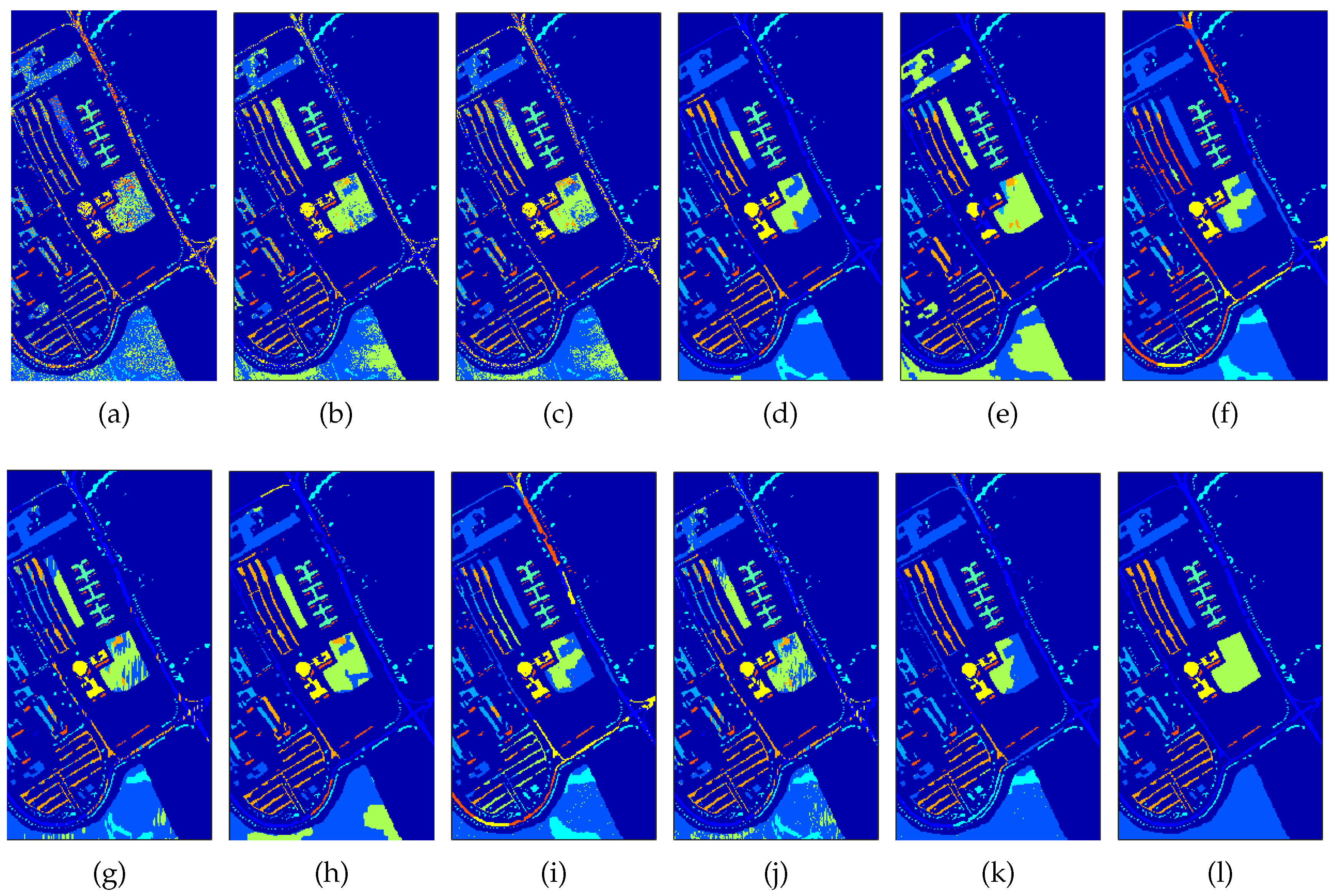
Figure 8 shows the obtained classification maps from the different methods. We can observe that the single source methods based on only spectral information, SunSAL and MLR produce noisy classification maps. The methods in which spatial information is included through MRF or CRF regularization: MRF_a, MRF_p, CRF_a and CRF_p already yield smoother classification maps. Finally, the methods that perform fusion of both modalities: MRFG, MRFG_a, MRFL and CRFL generated the best classification maps. The CRFL obtained the map closest to the ground truth map. From the table and the figure, one can also notice that MRFG_a performs better than MRFG, so we can conclude that the direct use of the abundances is superior to the use of probabilities obtained from the abundances.

(b) Indian Pines dataset

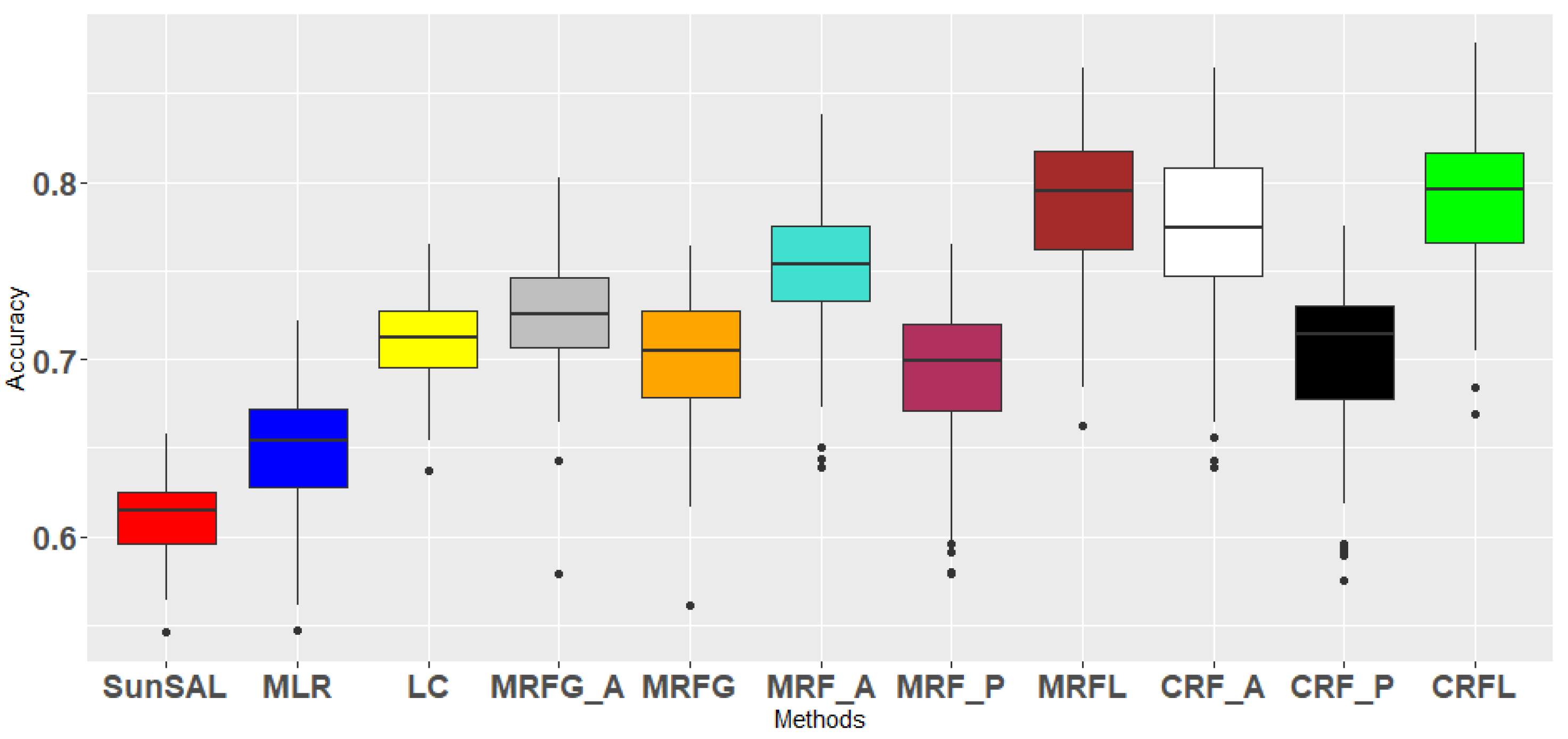
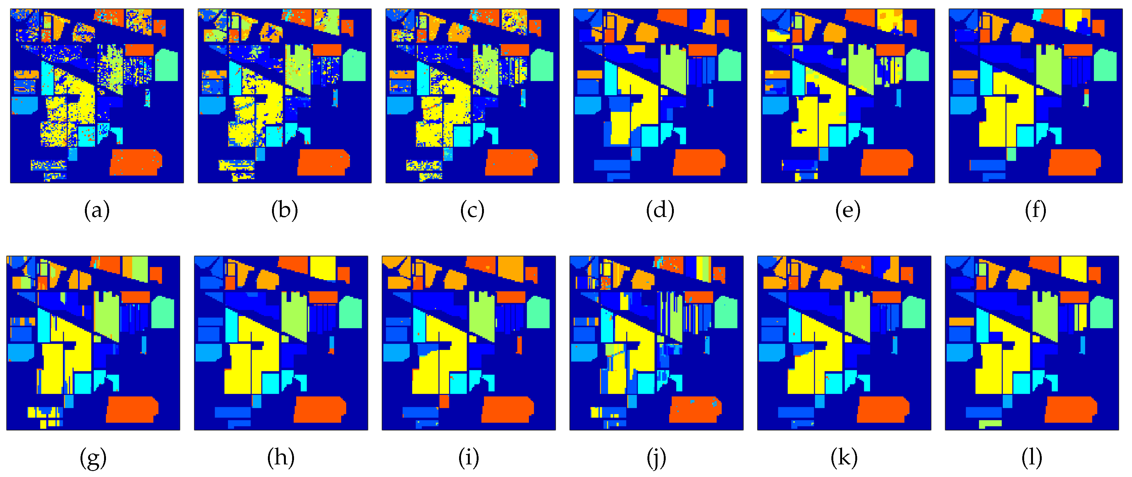
Quantitative results from the Indian Pines image are summarized in

Table 3. Classification accuracies [%] with their standard deviations for the Indian Pines image (the highest accuracies are denoted in bold).

Class	Train	Test	SunSAL	MLR	LC	MRFG_a	MRFG	MRF_a	MRF_p	MRFL	CRF_a	CRF_p	CRFL
Corn-notill	10	1418	53.97 $\pm 10.00$	55.83 $\pm 8.32$	64.71 $\pm 8.82$	61.85 $\pm 14.10$	58.39 $\pm 14.90$	70.13 $\pm 12.80$	60.96 $\pm 9.60$	75.12$\pm 11.05$	73.01 $\pm 14.73$	63.27 $\pm 10.30$	74.50 $\pm 10.78$
Corn-mintill	10	820	43.20 $\pm 10.00$	59.15 $\pm 8.87$	59.57 $\pm 10.33$	68.86 $\pm 12.50$	63.91 $\pm 13.00$	58.74 $\pm 16.20$	66.48 $\pm 10.70$	69.46 $\pm 14.90$	60.00 $\pm 20.30$	65.64 $\pm 11.50$	69.53$\pm 14.80$
Grass pasture	10	473	81.02 $\pm 6.20$	82.41 $\pm 8.76$	84.83 $\pm 6.64$	89.50$\pm 5.90$	89.27 $\pm 5.50$	80.52 $\pm 7.40$	84.23 $\pm 9.90$	82.38 $\pm 8.50$	78.97 $\pm 7.60$	83.49 $\pm 10.20$	81.60 $\pm 8.10$
Grass trees	10	720	88.24 $\pm 4.73$	91.75 $\pm 3.77$	96.12 $\pm 2.07$	97.31 $\pm 2.40$	96.47 $\pm 2.50$	98.45 $\pm 2.30$	95.66 $\pm 3.70$	99.52$\pm 1.40$	99.15 $\pm 1.60$	94.94 $\pm 3.74$	98.94 $\pm 1.80$
Hey Windrowed	10	468	99.62 $\pm 0.43$	99.82 $\pm 0.47$	100$\pm 0.03$	100$\pm 0.00$	100$\pm 0.00$	100$\pm 0.00$	99.98 $\pm 0.14$	100$\pm 0.00$	100$\pm 0.00$	99.9 $\pm 0.28$	100$\pm 0.00$
Soybean-notill	10	962	49.08 $\pm 9.04$	58.56 $\pm 11.69$	64.28 $\pm 6.74$	68.50 $\pm 12.90$	65.87 $\pm 13.80$	71.24 $\pm 8.90$	64.85 $\pm 12.00$	75.23 $\pm 5.10$	75.81 $\pm 6.20$	68.74 $\pm 11.77$	76.47$\pm 3.70$
Soybean-mintill	10	2445	47.98 $\pm 10.18$	48.15 $\pm 10.78$	55.24 $\pm 9.42$	55.83 $\pm 12.00$	53.76 $\pm 12.40$	62.88 $\pm 15.60$	51.54 $\pm 11.70$	65.73 $\pm 13.80$	66.07 $\pm 18.80$	53.47 $\pm 12.85$	67.80$\pm 14.90$
Soybean-clean	10	583	64.55 $\pm 10.58$	62.75 $\pm 8.96$	79.55 $\pm 10.07$	77.18 $\pm 12.06$	72.54 $\pm 12.54$	81.72 $\pm 15.50$	69.10 $\pm 10.42$	89.05$\pm 11.70$	86.19 $\pm 16.60$	71.23 $\pm 10.11$	88.20 $\pm 12.20$
Woods	10	1255	78.41 $\pm 8.94$	84.04 $\pm 8.11$	88.39 $\pm 6.23$	89.85 $\pm 8.20$	89.00 $\pm 9.00$	91.99 $\pm 8.70$	87.04 $\pm 8.50$	92.38 $\pm 7.10$	92.34 $\pm 8.90$	86.32 $\pm 8.73$	92.42$\pm 7.30$
Buildings	10	376	56.36 $\pm 9.96$	59.92 $\pm 6.61$	63.48 $\pm 7.00$	71.54 $\pm 9.20$	69.24 $\pm 9.70$	70.86 $\pm 13.40$	69.30 $\pm 7.90$	80.12$\pm 12.49$	70.38 $\pm 16.60$	64.15 $\pm 7.42$	70.00 $\pm 12.64$
OA (OA-SD)	-	-	61.11 $\pm 2.43$	64.86 $\pm 3.47$	71.06 $\pm 2.29$	72.45 $\pm 3.40$	70.16 $\pm 3.35$	75.11 $\pm 3.70$	69.31 $\pm 3.90$	78.95 $\pm 3.66$	77.22 $\pm 4.67$	70.22 $\pm 4.26$	79.00$\pm 3.70$
AA (AA-SD)	-	-	66.21 $\pm 1.73$	70.23 $\pm 2.49$	75.62 $\pm 1.58$	78.04 $\pm 2.43$	75.85 $\pm 2.48$	78.65 $\pm 2.60$	74.90 $\pm 2.90$	82.90$\pm 2.38$	80.20 $\pm 3.20$	75.12 $\pm 2.90$	81.95 $\pm 2.30$
$\kappa$ ($\kappa$-SD)	-	-	0.55 $\pm 0.02$	0.59 $\pm 0.02$	0.66 $\pm 0.02$	0.68 $\pm 0.03$	0.65 $\pm 0.03$	0.71 $\pm 0.04$	0.65 $\pm 0.04$	0.75 $\pm 0.04$	0.73 $\pm 0.05$	0.66 $\pm 0.04$	0.75 $\pm 0.04$

and Figure 9. Obtained classification maps are shown in Figure 10. From this, similar conclusions to the University of Pavia image can be drawn. Notice that CRF_a performs quite well in this image. A Pairwise McNemar statistical test shows that the proposed methods perform significantly better than the other methods, with the exception of CRF_a.

We have repeated some of the experiments for larger numbers of training samples per class (20, 50, 100), and noticed that the differences between the methods became smaller. This indicates that the advantages of the proposed methods level out for larger training sizes.

3.3.3. Experiment 3: Comparison of Different Decision Sources

With this experiment, we study the effect of using different decision sources in a pairwise manner in the proposed fusion frameworks. Three types of pairwise sources were applied for the MRFL and four for the CRFL:

• Pair 1: probabilities based on the spectra and probabilities based on the fractional abundances.
  The first source is the same as in the previous experiments and the fractional abundances were obtained using SunSAL. Subsequently, the abundances were used as input to an MLR classifier, to produce posterior classification probabilities for this set. Ultimately, these two sources of information were fused with the proposed MRFL and CRFL fusion schemes. Therefore, the only difference with the previous experiment is that, instead of the abundances, classification probabilities from the abundances are used.
• Pair 2: probabilities based on morphological profiles and probabilities based on the fractional abundances. Initially, (partial) morphological profiles were extracted as in [6] and used as input to an MLR classifier, to produce posterior classification probabilities. These were fused with the probabilities from the abundances using the proposed MRFL and CRFL fusion schemes. The difference with before is that the morphological profiles contain spatial-spectral information.
• Pair 3: probabilities based on morphological profiles and probabilities based on the spectra.
• Pair 4: For the CRFL pairwise fusion, we conducted one additional pairwise fusion, between the the pure fractional abundances and the probabilities based on the morphological profiles.

The pairwise fusion results in terms of OA and their standard deviations for the University of Pavia and Indian Pines datasets are displayed in

Table 4. Pairwise Fusion classification accuracies [%] using different pairwise decision sources.

	MRF_Pair1	MRF_Pair2	MRF_Pair3	CRF_Pair1	CRF_Pair2	CRF_Pair3	CRF_Pair4
University of Pavia	74.70 $\pm 5.00$	80.59 $\pm 3.70$	80.69 $\pm 3.80$	76.73 $\pm 5.00$	78.50 $\pm 4.12$	79.07 $\pm 4.03$	83.22 $\pm 4.10$
Indian Pines	76.51 $\pm 3.73$	77.70 $\pm 2.70$	77.26 $\pm 2.91$	73.70 $\pm 3.29$	73.25 $\pm 2.87$	74.70 $\pm 2.90$	77.03 $\pm 2.72$

.

We will now discuss the results from the table. The following conclusions can be drawn:

• In general, accuracies go down when the abundances are not directly used, but, instead, class probabilities are calculated from them (Pair 1).
• For the University of Pavia image, accuracies slightly improve when the spectral features are replaced by contextual features, but part of the effect disappears again because of the above-mentioned effect (Pair 2 and Pair 3). The best result is obtained with a direct use of abundances along with contextual features (CRF_Pair4).
• For the Indian Pines image, no improvement is observed when including contextual features.

3.3.4. Experiment 4: Additional Sources in the Fusion Framework

The proposed fusion framework is flexible in the sense that additional feature sources can be included. This experiment investigates the case where an additional third source/modality, on top of the two existing modalities, preferably including features which contain spatial information, is included in our fusion framework. Along with the two decision sources (i.e., the abundances obtained by SunSAL, and the probabilities derived from the initial spectra by using MLR classification), the probabilities derived from the morphological features are included as an additional source.

As before, each source has its own unary potentials. To not increase the complexity too much, we decided to retain the number of parameters. The three binary potential terms, one for each decision source, connecting neighboring pixels, are all jointly controlled by one parameter $\beta$. Now, three cross-link terms are required, connecting all combinations of pairs of decision sources. These are jointly controlled by one parameter $\gamma$. Ultimately, labels are produced for each source separately. A majority voting rule is applied in order to produce the resulting labels.

The classification accuracies are shown in

Table 5. Classification accuracies [%] based on the fusion of three sources (fractional abundances, probabilities based on spectra and probabilities based on morphological profiles) for the University of Pavia and Indian Pines images.

	MRFL_3	CRFL_3
University of Pavia	83.52 $\pm 3.52$	88.51 $\pm 3.87$
Indian Pines	82.85 $\pm 2.62$	82.16 $\pm 2.77$

for both datasets. The results reveal that a straightforward extension of the fusion framework with additional informative decision sources leads to an improvement of the classification accuracies.

4. Conclusions

In this paper, we proposed two novel decision fusion methodologies for hyperspectral image classification in remote sensing, addressing the high dimensionality versus the scarcity of ground truth information, the mixture of materials present in pixels and the collinearity of spectra in realistic scenarios. The decision fusion framework is based on probabilistic graphical models, MRFs and CRFs, with a specific selection of complementary decision sources: (1) fractional abundances, obtained by sparse unmixing, facilitating the characterization of the subpixel content in mixed pixels, and (2) probabilistic outputs from a soft classifier, expressing confidence about the spectral content of the pixels. Furthermore, the methods simultaneously take into account two types of relationships between the underlying variables: (a) spatial neighborhood dependencies between the pixels—and (b) consistency between the two decision sources. Experiments on two real hyperspectral datasets with limited training data demonstrated the performance of the framework. The fractional abundances were shown to generate an informative decision source. Both methods MRFL and CRFL outperformed other fusion approaches when applied to the same decision sources. The fusion method CRFL produced high overall accuracies, and was stable over a large range of parameter values. Finally, the addition of a third decision source improved the classification accuracies. In future work, the aim is to further improve the classification accuracies by including additional parameter learning to estimate the model parameters directly from the training data.

References

- Hughes, G. On the Mean Accuracy of Statistical Pattern Recognizers. IEEE Trans. Inf. Theor. 2006, 14, 55–63. [Google Scholar] [CrossRef]
- Plaza, A.; Martinez, P.; Plaza, J.; Perez, R. Dimensionality reduction and classification of hyperspectral image data using sequences of extended morphological transformations. IEEE Trans. Geosci. Remote Sens. 2005, 43, 466–479. [Google Scholar] [CrossRef] [Green Version]
- Dalla Mura, M.; Benediktsson, J.A.; Waske, B.; Bruzzone, L. Extended profiles with morphological attribute filters for the analysis of hyperspectral data. Int. J. Remote Sens. 2010, 31, 5975–5991. [Google Scholar] [CrossRef]
- Liao, W.; Bellens, R.; Pizurica, A.; Philips, W.; Pi, Y. Classification of Hyperspectral Data Over Urban Areas Using Directional Morphological Profiles and Semi-Supervised Feature Extraction. IEEE J. Sel. Top. Appl. Earth Obs. Remote Sens. 2012, 5, 1177–1190. [Google Scholar] [CrossRef]
- Benediktsson, J.A.; Palmason, J.A.; Sveinsson, J.R. Classification of hyperspectral data from urban areas based on extended morphological profiles. IEEE Trans. Geosci. Remote Sens. 2005, 43, 480–491. [Google Scholar] [CrossRef]
- Liao, W.; Chanussot, J.; Dalla Mura, M.; Huang, X.; Bellens, R.; Gautama, S.; Philips, W. Taking optimal advantage of fine spatial information: promoting partial image reconstruction for the morphological analysis of very-high-resolution images. IEEE Geosci. Remote Sens. Mag. 2017, 5, 8–28. [Google Scholar] [CrossRef]
- Licciardi, G.; Marpu, P.R.; Chanussot, J.; Benediktsson, J.A. Linear versus nonlinear PCA for the classification of hyperspectral data based on the extended morphological profiles. IEEE Geosci. Remote Sens. Lett. 2012, 9, 447–451. [Google Scholar] [CrossRef]
- Song, B.; Li, J.; Dalla Mura, M.; Li, P.; Plaza, A.; Bioucas-Dias, J.M.; Benediktsson, J.A.; Chanussot, J. Remotely sensed image classification using sparse representations of morphological attribute profiles. IEEE Trans. Geosci. Remote Sens. 2014, 52, 5122–5136. [Google Scholar] [CrossRef]
- Fauvel, M.; Benediktsson, J.; Chanussot, J.; Sveinsson, J. Spectral and spatial classification of hyperspectral data using SVMs and morphological profiles. IEEE Trans. Geosci. Remote Sens. 2008, 46, 3804–3814. [Google Scholar] [CrossRef]
- Tuia, D.; Matasci, G.; Camps-Valls, G.; Kanevski, M. Learning the relevant image features with multiple kernels. In Proceedings of the 2009 IEEE International Geoscience and Remote Sensing Symposium, Cape Town, South Africa, 12–17 July 2009; Volume 2, pp. II-65–II-68. [Google Scholar]
- Li, J.; Huang, X.; Gamba, P.; Bioucas-Dias, J.M.; Zhang, L.; Benediktsson, J.A.; Plaza, A.J. Multiple feature learning for hyperspectral image classification. IEEE Trans. Geosci. Remote Sens. 2015, 53, 1592–1606. [Google Scholar] [CrossRef]
- Licciardi, G.; Pacifici, F.; Tuia, D.; Prasad, S.; West, T.; Giacco, F.; Thiel, C.; Inglada, J.; Christophe, E.; Chanussot, J.; et al. Decision fusion for the classification of hyperspectral data: outcome of the 2008 GRSS data fusion contest. IEEE Trans. Geosci. Remote Sens. 2009, 47, 3857–3865. [Google Scholar] [CrossRef]
- Song, B.; Li, J.; Li, P.; Plaza, A. Decision fusion based on extended multi-attribute profiles for hyperspectral image classification. In Proceedings of the 5th Workshop on Hyperspectral Image and Signal Processing: Evolution in Remote Sensing (WHISPERS), Gainesville, FL, USA, 26–28 June 2013. [Google Scholar]
- Li, W.; Prasad, S.; Tramel, E.W.; Fowler, J.E.; Du, Q. Decision fusion for hyperspectral image classification based on minimum-distance classifiers in the wavelet domain. In Proceedings of the 2014 IEEE China Summit & International Conference on Signal and Information Processing (ChinaSIP), Xi’an, China, 9–13 July 2014; pp. 162–165. [Google Scholar]
- Benediktsson, J.A.; Kanellopoulos, I. Classification of multisource and hyperspectral data based on decision fusion. IEEE Trans. Geosci. Remote Sens. 1999, 37, 1367–1377. [Google Scholar] [CrossRef] [Green Version]
- Kalluri, H.R.; Prasad, S.; Bruce, L.M. Decision-level fusion of spectral reflectance and derivative information for robust hyperspectral land cover classification. IEEE Trans. Geosci. Remote Sens. 2010, 48, 4047–4058. [Google Scholar] [CrossRef]
- Yang, H.; Du, Q.; Ma, B. Decision fusion on supervised and unsupervised classifiers for hyperspectral imagery. IEEE Geosci. Remote Sens. Lett. 2010, 7, 875–879. [Google Scholar] [CrossRef]
- Li, S.; Lu, T.; Fang, L.; Jia, X.; Benediktsson, J.A. Probabilistic fusion of pixel-level and superpixel-level hyperspectral image classification. IEEE Trans. Geosci. Remote Sens. 2016, 54, 7416–7430. [Google Scholar] [CrossRef]
- Khodadadzadeh, M.; Li, J.; Ghassemian, H.; Bioucas-Dias, J.; Li, X. Spectral-spatial classification of hyperspectral data using local and global probabilities for mixed pixel characterization. IEEE Trans. Geosci. Remote Sens. 2014, 52, 6298–6314. [Google Scholar] [CrossRef]
- Khodadadzadeh, M.; Li, J.; Plaza, A.; Ghassemian, H.; Bioucas-Dias, J.M. Spectral-spatial classification for hyperspectral data using SVM and subspace MLR. In Proceedings of the 2013 IEEE International Geoscience and Remote Sensing Symposium—IGARSS, Melbourne, Australia, 21–26 July 2013; pp. 2180–2183. [Google Scholar]
- Xia, J.; Chanussot, J.; Du, P.; He, X. Spectral–spatial classification for hyperspectral data using rotation forests with local feature extraction and markov random fields. IEEE Trans. Geosci. Remote Sens. 2015, 53, 2532–2546. [Google Scholar] [CrossRef]
- Lu, Q.; Huang, X.; Li, J.; Zhang, L. A novel MRF-based multifeature fusion for classification of remote sensing images. IEEE Geosci. Remote Sens. Lett. 2016, 13, 515–519. [Google Scholar] [CrossRef]
- Lu, T.; Li, S.; Fang, L.; Jia, X.; Benediktsson, J.A. From subpixel to superpixel: a novel fusion framework for hyperspectral image classification. IEEE Trans. Geosci. Remote Sens. 2017, 55, 4398–4411. [Google Scholar] [CrossRef]
- Gómez-Chova, L.; Tuia, D.; Moser, G.; Camps-Valls, G. Multimodal classification of remote sensing images: a review and future directions. Proc. IEEE 2015, 103, 1560–1584. [Google Scholar] [CrossRef]
- Solberg, A.H.S.; Taxt, T.; Jain, A.K. A markov random field model for classification of multisource satellite imagery. IEEE Trans. Geosci. Remote Sens. 1996, 34, 100–113. [Google Scholar] [CrossRef]
- Wegner, J.D.; Hansch, R.; Thiele, A.; Soergel, U. Building detection from one orthophoto and high-resolution InSAR data using conditional random fields. IEEE J. Sel. Top. Appl. Earth Obs. Remote Sens. 2011, 4, 83–91. [Google Scholar] [CrossRef]
- Albert, L.; Rottensteiner, F.; Heipke, C. A higher order conditional random field model for simultaneous classification of land cover and land use. Int. J. Photogramm. Remote Sens. 2017, 130, 63–80. [Google Scholar] [CrossRef]
- Tuia, D.; Volpi, M.; Moser, G. Decision fusion with multiple spatial supports by conditional random fields. IEEE Trans. Geosci. Remote Sens. 2018, 56, 3277–3289. [Google Scholar] [CrossRef]
- Bioucas-Dias, J.; Figueiredo, M. Alternating direction algorithms for constrained sparse regression: Application to hyperspectral unmixing. In Proceedings of the 2nd Workshop on Hyperspectral Image and Signal Processing: Evolution in Remote Sensing (WHISPERS), Reykjavik, Iceland, 14–16 June 2010. [Google Scholar]
- Dopido, I.; Li, J.; Gamba, P.; Plaza, A. A new hybrid strategy combining semisupervised classification and unmixing of hyperspectral data. IEEE J. Sel. Top. Appl. Earth Obs. Remote Sens. 2014, 7, 3619–3629. [Google Scholar] [CrossRef]
- Chen, Y.; Nasrabadi, N.M.; Tran, T.D. Hyperspectral image classification using dictionary-based sparse representation. IEEE Trans. Geosci. Remote Sens. 2011, 49, 3973–3985. [Google Scholar] [CrossRef]
- Li, W.; Du, Q. Joint within-class collaborative representation for hyperspectral image classification. IEEE J. Sel. Top. Appl. Earth Obs. Remote Sens. 2014, 7, 2200–2208. [Google Scholar] [CrossRef]
- Sun, X.; Qu, Q.; Nasrabadi, N.M.; Tran, T.D. Structured priors for sparse-representation-based hyperspectral image classification. IEEE Geosci. Remote Sens. Lett. 2014, 11, 1235–1239. [Google Scholar]
- Bishop, C.M. Pattern Recognition and Machine Learning; Springer: Berlin/Heidelberg, Germany, 2006. [Google Scholar]
- Scheunders, P.; Tuia, D.; Moser, G. Contributions of machine learning to remote sensing data analysis. In Comprehensive Remote Sensing; Liang, S., Ed.; Elsevier: Amsterdam, The Netherlands, 2017; Volume 2, Chapter 10. [Google Scholar]
- Hastie, T.; Tibshirani, R.; Friedman, J. The Elements of Statistical Learning; Springer: New York, NY, USA, 2009. [Google Scholar]
- Namin, S.T.; Najafi, M.; Salzmann, M.; Petersson, L. A multi-modal graphical model for scene analysis. In Proceedings of the 2015 IEEE Winter Conference on Applications of Computer Vision, Waikoloa, HI, USA, 5–9 January 2015; pp. 1006–1013. [Google Scholar] [CrossRef]
- Boykov, Y.; Kolmogorov, V. An experimental comparison of min-cut/max-flow algorithms for energy minimization in vision. IEEE Trans. Pattern Anal. Mach. Intell. 2004, 26, 1124–1137. [Google Scholar] [CrossRef]
- Boykov, Y.; Veksler, O.; Zabih, R. Fast approximation energy minimization via graph cuts. IEEE Trans. Pattern Anal. Mach. Intell. 2001, 23, 1222–1239. [Google Scholar] [CrossRef]
- Kohli, P.; Ladicky, L.; Torr, P. Robust higher order potentials for enforcing label consistency. Int. J. Comp. Vis. 2009, 82, 302–324. [Google Scholar] [CrossRef]
- Kohli, P.; Ladicky, L.; Torr, P. Graph Cuts for Minimizing Robust Higher Order Potentials; Technical Report; Oxford Brookes University: Oxford, UK, 2008. [Google Scholar]
- Boykov, Y.; Jolly, M.P. Interactive graph cuts for optimal boundary and region segmentation of objects in n-D images. In Proceedings of the Eighth IEEE International Conference on Computer Vision, Vancouver, BC, Canada, 7–14 July 2001. [Google Scholar]
- Weinmann, M.; Schmidt, A.; Mallet, C.; Hinz, S.; Rottensteiner, F.; Jutzi, B. Contextual classification of point cloud data by exploiting individual 3D neighborhoods. ISPRS Ann. Photogramm. Remote Sensi. Spat. Inf. Sci. 2015, II-3/W4, 271–278. [Google Scholar] [CrossRef]
- Iordache, M.D.; Bioucas-Dias, J.; Plaza, A. Collaborative sparse regression for hyperspectral unmixing. IEEE Trans. Geosci. Remote Sens. 2013, 52, 341–354. [Google Scholar] [CrossRef]
- Iordache, M.D.; Bioucas-Dias, J.; Plaza, A. Total variation spatial regularization for sparse hyperspectral unmixing. IEEE Trans. Geosci. Remote Sens. 2012, 50, 4484–4502. [Google Scholar] [CrossRef]
Figure 1.
The graph representation of MRFL. Green nodes denote the random variables associated with , blue nodes denote the random variables associated with . Black lines denote the edges that model the spatial neighborhood dependencies. Red lines denote the cross links between and , encoding the potential interactions . is the parameter that controls the influence of these interaction terms.
Figure 2.
Graph representation of CRFL. The purple nodes denote random variables associated with the observed data, the green nodes denote random variables associated with the labels , blue nodes denote random variables associated with the labels . The turqoise lines denote the link of the labels with the observed data. Black lines denote the edges that model the spatial neighborhood dependencies. Red lines denote the cross links between and encoding the potential interactions . is the parameter that controls the influence of these interaction terms.
Figure 3.
University of Pavia: (a) false color composite image (R:40,G:20,B:10); (b) ground reference map.
Figure 4.
Indian Pines: (a) RGB image; (b) ground reference map.
Figure 5.
Effect of and on the Overal Accuracy (OA) for both proposed methods: MRFL and CRFL.
Figure 6.
Confusion matrices between (a) SunSAL and the MLR classifier on the University of Pavia image; (b) the SVM and the MLR classifier on the University of Pavia image; (c) SunSAL and the MLR classifier on the Indian Pines image; (d) the SVM and the MLR classifier on the Indian Pines image.
Figure 7.
Boxplot from Overall Accuracies (OA) for several methods on the University of Pavia image, including the proposed ones: MRFL and CRFL (100 experiments).
Figure 8.
University of Pavia classification maps generated from different methods; (a) SunSAL, (b) MLR, (c) LC, (d) MRFG_a, (e) MRFG, (f) MRF_a, (g) MRF_p, (h) MRFL, (i) CRF_a, (j) CRF_p, (k) CRFL, (l) Ground truth.
Figure 9.
Boxplot from Overal Accuracies (OA) for several methods on the Indian Pines image including the proposed ones: MRFL and CRFL (100 experiments).
Figure 10.
Indian Pines classification maps generated from different methods. (a) SunSAL, (b) MLR, (c) LC, (d) MRFG_a, (e) MRFG, (f) MRF_a, (g) MRF_p, (h) MRFL, (i) CRF_a, (j) CRF_p, (k) CRFL, (l) Ground truth.