Storm Event to Seasonal Evolution of Nearshore Bathymetry Derived from Shore-Based Video Imagery
by
 , , and
Erwin W. J. Bergsma
1,*,† ,
,
Daniel C. Conley
2,
Mark A. Davidson
2,
Tim J. O'Hare
2 and
Rafael Almar
3 1
CNES-LEGOS, UMR-5566, 14 Avenue Edouard Belin, 31400 Toulouse, France
2
CPRG, School of Biological and Marine Sciences, University of Plymouth, Drake Circus, Plymouth PL4 8AA, UK
3
IRD-LEGOS, UMR-5566, 14 Avenue Edouard Belin, 31400 Toulouse, France
*
Author to whom correspondence should be addressed.
†
Current address: Laboratoire d’Etudes en Géophysique et Océanographie Spatiales (LEGOS), 14 Avenue Edouard Belin, 31400 Toulouse, France.
Remote Sens. 2019, 11(5), 519; https://doi.org/10.3390/rs11050519
Submission received: 22 January 2019
/
Revised: 22 February 2019
/
Accepted: 26 February 2019
/
Published: 4 March 2019
(This article belongs to the Section Ocean Remote Sensing)
Abstract
:Coastal evolution occurs on a wide range of time-scales, from storms, seasonal and inter-annual time-scales to longer-term adaptation to changing environmental conditions. Measuring campaigns typically either measure morphological evolution on a short-time scale (days) with high frequency (hourly) or long-time scales (years) but intermittently (monthly). This leaves an important observational gap that limits morphological variability assessments. Traditional echo sounding measurements on this long time-scale and high-frequency sampling require a significant financial injection. Shore-based video systems with high spatiotemporal resolution can bridge this gap. For the first time, hourly Kalman filtered video-derived bathymetries covering 1.5 years of morphological evolution with an hourly resolution obtained at Porhtowan, UK are presented. Here, the long-term hourly dataset is used and aims to show its added value for, and provide an in-depth, morphological analyses with unprecedented temporal resolution. The time-frame includes calm and extreme (storm) wave conditions in a macro-tidal environment. The video-derived bathymetries allow hourly beach state classification while before this was not possible due to the dependence on foam patterns of wave breaking (e.g., saturation during storms). The study period covers extreme storm erosion during the most energetic winter season in 60 years (2013–2014). Recovery of the beach takes place on several time-scales: (1) an immediate initial recovery after the storm season (first 2 months), (2) limited recovery during low energetic summer conditions and (3) accelerated recovery as the wave conditions picked up in the subsequent fall—under wave conditions that are typically erosive. The video-derived bathymetries are shown to be effective in determining bar-positions, outer-bar three-dimensionality and volume analyses with an unprecedented hourly temporal resolution.
1. Introduction
Intensifying and more frequent storms and corresponding increased coastal water levels [1] and wave conditions [2], affect the usability, economic value and protection of the world coastal areas [3]. More variable and intense meteorological conditions lead to more severe wave conditions in the coastal zone [2,4,5]. Intense wave conditions during storms generally have an episodic resetting effect on nearshore beach morphology [6,7]. Phillips et al. [7] shows that Narrabeen beach (Australia) tends to accumulate sediment over months during calm conditions, while during storms beaches erode large sediment quantities in a matter of days [7]. The conceptual beach state model of Wright and Short [8] helps to classify morphological behaviour. For example, during energetic wave conditions, beaches evolve up-state towards ultimately a dissipative beach state (following [8]). Sediment is typically transported and deposited offshore during a storm. Sediment is subsequently slowly transported back to shore under moderate-to-calm wave conditions [7] and beaches evolve down-state (towards ultimately a reflective state). Effectively, the morphological behaviour of a beach can hardly be linked to a single time-scale and should often be considered a combination of time-scales ranging from events (days) to a longer term such as seasonal or inter-annual [9]. It is this variety of spatiotemporal morphological scales that traditionally introduces a difficulty in obtaining measurements that cover them all. As a rule of thumb with only very few exceptions (such as the Field Research Facility (FRF) at Duck, NC), we can scale the duration and repetition of a field campaign to the morphological scale one attempts to observe. For example, high resolution/frequency measurements for small-scale processes are carried out over short periods [10,11] and vice versa for large-scale less frequent measurements [12,13,14,15,16] but with our present state-of-the-art set of measuring tools, it is still thought challenging to cover all the scales with a single conventional tool. This leads to important data gaps and consequent knowledge gaps.
Several long-term datasets exist mostly covering the inter-tidal beach area [12,13,14,15,16]. Measurements are often taken on a bi-monthly to a monthly basis and/or the most energetic periods are covered with a pre- and post-storm measurement. Smaller temporal scale morphological variations are not resolved due to the intermittent nature of existing datasets. Also, short intensive field campaigns typically obtain greatly detailed measurements, but over a short period. In addition, storm morphology is typically hard to capture due to powerful environmental conditions during storms. In-situ measuring devices to obtain bathymetries do not endure such conditions or require calm conditions to function properly. For instance, traditional bathymetry measurements using an echo-sounder require an almost flat sea state in the near-shore. A result is the lack of qualitative and appropriate observational storm response datasets (with measurements before and after the storm). Datasets are required that can be used to understand morphological evolution under storm conditions and validate (numerical) models for their performance on storm response predictions and hindcasting [17,18]. Furthermore, Ref. [19] showed that field observations are rarely sufficient to numerically predict future storm response in, for example, early warning systems (EWS). Recent developments in remotely sensing nearshore bathymetry, its error estimation [20] and data assimilation [21,22] should be able to fill this data-gap, using X-band radar [23] or video-imagery.
Nearshore video-imagery observation has been used in the past to assess storm impact, in particular, bar migration and straightening of bar systems under storm conditions e.g., [24,25,26,27]. Bathymetries are traditionally measured by ship-mounted echo-sounders that measure the time of flight of an acoustic pulse to estimate the depth. Remotely sensed bathymetry estimation was enhanced during the late 1990s to 2000s [28,29,30,31] but remained sensitive to the complexity of the nearshore bathymetry. For shore-based video-camera systems, Almar et al. [32] introduced a temporal cross-correlation technique to estimate bathymetries, which is later extended with an independent error estimation [20] that is proven to work in more energetic wave conditions and complex bar morphology. At the same time, Ref. [33] showed a renewed and robust spectral depth-inversion technique based on a spectral phase shift method [30] to estimate ocean wavenumbers and subsequently derive depth. Holman et al. [34] extended the latter cross-shore method to a third (alongshore) dimension and introduced data assimilation (through a Kalman filter) to reduce the effect of instantinous inversion errors, enabling robust capturing of temporal nearshore morphology. This method is now tested and operational at various sites in different wave and tidal environments [34,35,36,37]. Here, the method is modified for energetic macro-tidal environments, following Bergsma et al. [35]. Under energetic wave conditions and large tidal ranges, depths are generally estimated with a spatially varying accuracy of tens of centimetres; a mean error of 3 cm and 60 cm standard deviation [35]. Similar accuracy has been found in Holman et al. [34], Sembiring et al. [38] and Brodie et al. [37]. These numbers are of a similar order in comparison to echo-sounders used in challenging conditions inherent to the nearshore area.
This work aims to show the added value of video-derived bathymetries and provide an in-depth analysis of 1.5-year morphological change using video-derived bathymetry estimations. We present the first study that observes hourly Kalman-filtered two-dimensional morphological evolution at Porthtowan in the United Kingdom (see Table A3 in Appendix B). This enables analysis of spatial and temporal links between morphological scales; from rapid storm-impact to slow recovery, from a featureless beach to complex morphological beach states. A long-term video-derived bathymetry dataset including a detailed observation of nearhore morphology under (extreme) storm and calm wave conditions at Porthtowan, the United Kingdom from October 2013 to February 2015 is presented. This paper presents multi-scale resolving capabilities of video-based bathymetry estimation. Hourly bathymetry estimation opens-up the possibility of analysing beach erosion or accumulation at an unprecedented hourly resolution.
2. Methods
2.1. Study Site
A series of studies were launched in 2008 under the “wave hub” renewable energy test site framework [www.wavehub.co.uk] to investigate the effect of renewable energy devices on the marine environment. The beach at Porthtowan, located in South–West England, was selected to be one of the test sites as it is situated in the presumed lee of the wave hub. Rocky outcrop/geology bounds the beach on the landward side Figure 1. During high-tide conditions, the water level rises to the rocky outcrop. Depending on the time of year the eight-year average beach-state varies between “barred” (November to March) to “low tide bar-rip” (April to October) [39] considering a median sediment size () 380 μm [40,41].
Monthly inter-tidal beach measurements started in 2008 and continued until 2016. The inter-tidal beach levels were measured using real time kinematic (RTK) GPS mounted on an all-terrain vehicle (ATV). Occasionally, for example in between storms, extra topography measurements were carried out to map storm impact. The beach topography measurements were typically executed on the day of the largest spring tidal range for that month. Simultaneously with the start of monthly beach surveys, an “Argus” video camera system [42] was installed. Over the complete time-frame, the Argus system delivered primary products such as snapshot, Timex (10-min TIMe EXposure) and variance images of the beach. These primary image-products are typically projected on a horizontal plane to provide a birds-eye view. Secondary products such as depth inversion derived bathymetries were introduced in early 2013. Hence, for the present study, we are limited to a shorter time-frame than the total inter-tidal beach dataset. This work, therefore, covers the period from October 2013 until February 2015. In addition, echo-sounder bathymetry surveys were carried out intermittently between 2008 and 2016. Termination of the monthly topography measurements in 2016 meant that, at the same time, the Argus system was phased out.
2.2. Wave and Tidal Data
Hourly significant wave height (), peak-period (), zero-crossing period () and direction () were obtained with an inshore Datawell Directional WaveRider Mk III buoy 5 km North of Porthtowan. Detailed wave statistics can be found in Appendix A, covering a period from 2008 to 2017. At Porthtowan, we found an average significant wave height of 1.57 m, average peak period of 10.51 seconds with an average incident direction of 283.4 degrees (W–NW). The wave conditions at Porthtowan vary significantly between winter (more energetic) and summer (calmer) months as Table A2 reveals. Unfortunately, during the morphological time-frame analyzed here (2013–2015), the wave buoy was heavily damaged during an extreme storm on the 5 February 2014. Roughly a month later a replacement buoy was deployed at the same location. In absence of the wave buoy, a SWAN-model (Simulating WAve Nearshore) was used to compute local wave conditions. From the measured wave height and period, the total wave power was derived. Assuming the wave data is obtained in deep water, wave power can be found using (1).
in which represents density, g the gravitational acceleration, is the significant wave height, represent the energy period. The only parameter that is not directly obtained from the wave buoy is (commonly referred to as ). Cahill and Lewis [43] use a spectral relationship between the zero-crossing period () and the energy period to obtain the latter using (2).
In Equation (2) represents a wave period ratio () which spectral shape (denoted as ) reflects the instant wave climate. Here, we assume a further developing sea-state in the form of a JONSWAP spectrum, hence we use . Cahill and Lewis [43] show that the varies between 1.22 and 1.12 for ’s ranging between 1 and 10. For JONSWAP spectra is typically set to 3.3. Corresponding to , should be 1.18 according to the work of Cahill and Lewis [43].
The tidal constituents were derived from two years of in-situ pressure transducer time-series (at Porthtowan) by using the r-t-tide model [44]. The tidal range at Porthtowan was about 7 m. In addition to model tidal elevation, nearby atmospheric-pressure measurements (Perranporth Airport) were used to account for the inverse barometric effect which can be in the order of 10s of centimetres during storms.
2.3. Wave Conditions and Storm Identification
The video data (October 2013–February 2015) was collected during the most energetic winter in the last decade (2008–2017), as shown in Table A2. The average winter wave height in 2013–2014 was higher than the decade-average, and the average hourly wave incident wave power was 1.45 times the decade-average. In this work we specifically target the impact of storms and a sequence of storms. Storms are commonly identified using a peak over threshold (PoT) approach using the significant wave height e.g., [45,46,47]. Amongst others, Harley et al. [48] and Splinter et al. [49] used field data to show that volumetric change under storm conditions is a function of the incident wave power. Also, shoreline changes showed a good correlation with the incident wave energy flux (wave power), as shown by Davidson et al. [6]. Considering this intrinsic link, wave power seems to be a more suitable measure to identify storms for morphological purposes. Figure 2c,d show exceedance threshold values for wave power. These and quantile thresholds were derived in a similar way as to [47,50] but from wave power instead of wave height.
Over the study period, Figure 2 and Table 1 indicate that the most powerful storms occurred between January and February 2014. Four subsequent storms from 3 January to 1 February 2014, respectively, had a significantly greater accumulative power in comparison to the other storms during the same winter season. In addition, the degree of beach erosion was typically linked to the tidal range [17]; larger tidal range corresponding to greater beach erosion. Considering this, one can expect the largest impact from the storms on 3 January 2014 and 1st February as they coincide with tidal ranges of 6.6 and 7.0 m. The first storm of the 2014–2015 winter season occurred significantly later in comparison to 2013–2014. The first storm to arrive in fall 2014 was early December 2014. The wave power exceeded the quantile threshold for the second time that winter in mid-January 2015, at the end of our study period.
2.4. Video-Derived Bathymetries
Video-derived bathymetries are typically obtained by solving an inverse problem using a linear relationship between wave celerity and depth. The linear dispersion relation for free surface waves in Equation (3) is used to invert depths from pixel intensity time-stacks.
wherein c is wave celerity, t time, x represents absolute distance, angular wave frequency, k represents the wave number, g the gravitational acceleration, h depth, and represents the mean current. Field measurements were carried out by Merrifield and Guza [51] and Holland [52] showed that the current relative to the phase speed of the wave was small at open coasts and could, therefore, be neglected. Hydrodynamic results from a regional numerical model [53] suggested that tidal currents reduced by over 50% 1 km from the coast resulting in shore-parallel peak-currents with a magnitude 0.3 m/s or less. Apart from local embayed parts of the coast, tide-induced cross-shore currents seem absent [53]. Hence, allowing the current-term to be neglected here. This does not necessarily hold for wave-induced currents in the nearshore zone. Neglecting the mean wave-induced current in rip channels can lead to a 10– error as found in Almar et al. [54]. After rearranging Equation (3), depth can be found as a function of the wave celerity (c) resulting in Equation (4).
Following Equation (4), depth inversion requires knowledge of the wave celerity, either as in frequency space [30] or in temporal space wherein x in is the normal wave direction [32]. Thus, solving the inverse problem requires either k or (or similarly L or T, respectively as and ). Here, a spectral depth-inversion method cBathy [34] is used to obtain depth. cBathy is based on a spectral method of wave number retrieval from video imagery [33]. In order to invert depths using the right-hand side of (4), the spectral approach seeks to find a wave number (k) and associated frequency (). The total cBathy package consists of three phases. Phase I contains the estimation of N number of sets, where N is user-defined. The second phase of cBathy combines the N number of -sets into an optimal singular estimate for k, and hence depth (h) including an error estimation per depth estimate () that can be used in the following phase (assimilation). Phase III deploys a Kalman like filter to assimilate multiple estimated bathymetries in time and ultimately increase the accuracy [34].
The original version of cBathy (as described above) is modified to account for pixel movement and inter-camera boundary effects [35]. Here, the user-defined settings are identical to the settings used in [35]. The accuracy of the video-derived bathymetries depends on wave conditions. [34,37] showed that with increasing wave conditions the error of the estimation increases. One can imagine that the linear dispersion relation is valid to a lesser extent in the shallowest parts of the domain due to wave non-linearities [20,55]. The cross-shore extent for which bathymetry estimation is possible depends on the wave height and generally increases as wave conditions increase. Considering this only, we prefer small, short period waves for the shallowest part of the domain. The opposite applies for the deeper part where the small waves are in relatively deep water and wave-celerity is lesser limited by the local depth—hence we required more energetic long period waves to estimate the bathymetry correctly. Estimates with reasonable accuracy were obtained in deeper waters (20 m) during more energetic conditions at Porthtowan. However, the longer period incident waves inherently lead to a reduced capability of estimating relatively small (to the wavelength) morphological features. By combining several wave frequency/number sets and Kalman filtering these wave-condition related errors can be reduced. Under calm wave conditions (here, measured bathymetries were only available under calm conditions) the spatial average error obtained at Porthtowan is in the order of tens of centimetres which corresponds to of the water depth. For the ground-truth surveys, an RMS error of 3 cm with a standard deviation of 61 cm is found as presented in Bergsma et al. [35]. The errors varied spatially: largest scatter was found for depths greater than 12 m (the mean error is small) [39], where we find that depths were slightly underestimated. The opposite was found for the shallowest part of the domain at which relatively large errors can be found in the inter-tidal area (depths smaller than 0), similar error-patterns were found in [34,36].
2.5. Determination of the Bar Position
Until recently, shore-based video monitoring systems predominantly provided qualitative measures for beach morphology such as a shoreline and bar detection by the use of wave breaking induced foam patterns. Quantification of inter-tidal beach levels is possible by following the moving shoreline due to tides. Qualitative measures such as sub-tidal bar detection remained the only video-derived product to capture sub-tidal morphology. Foam patterns due to waves breaking over sub-tidal bars leave an indicator of the bar position and morphological state [24,56,57]. Thus, a bar position can be determined as a local cross-shore maximum in pixel intensity in the Timex imagery. The existence and cross-shore position of foam due to wave breaking depends on wave conditions and tidal elevation, and this variability should be accounted for accordingly [25,58]. Similarly, sub-tidal bar patterns can be identified for the estimated bathymetries as a local maximum bed level.
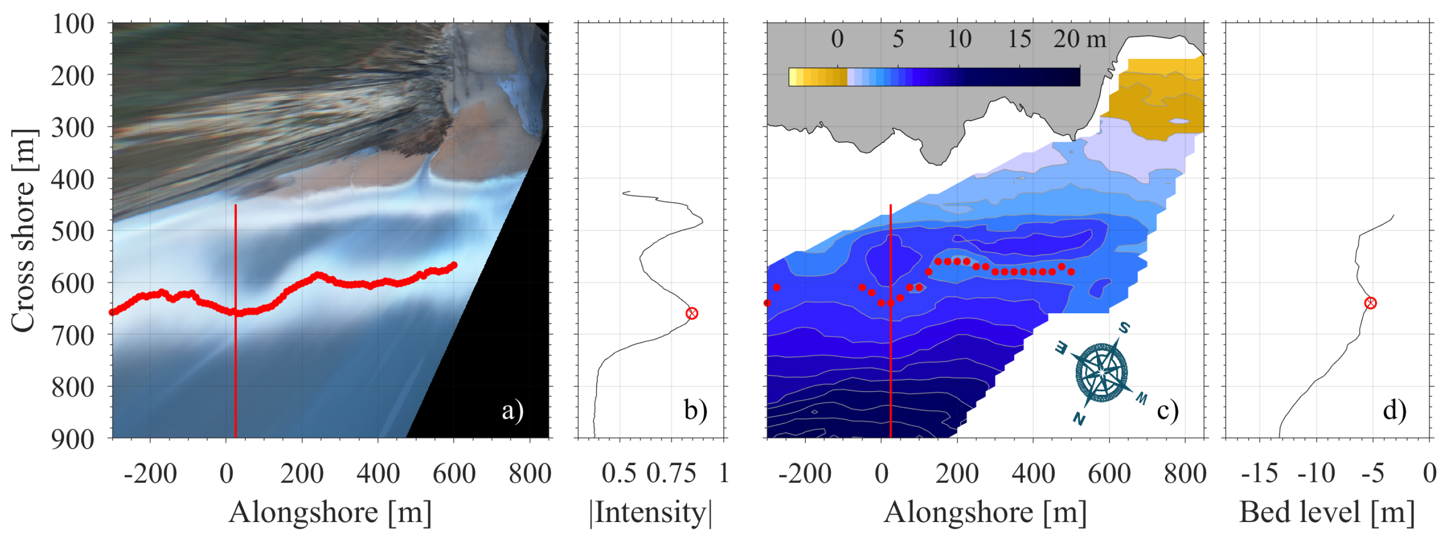
Bar detection from the Timex imagery is illustrated in Figure 3a,b. The detection scheme identifies cross-shore peaks in pixel intensities. For video-derived bathymetries, local maxima in the cross-shore bed level profile represent the sub-tidal bar position. An example of detected bar positions from video-derived bathymetry is shown in Figure 3c,d. Here, we are only interested in the outer bar, hence only the most offshore located peak is taken as the sub-tidal bar location, best illustrated in Figure 3b. Bar positions are detected every metre alongshore for the pixel intensity and every 10 m alongshore for the bathymetry estimates. Ultimately, an alongshore mean bar position and corresponding standard deviation are derived from these individual bar positions.
2.6. Cross-Shore Sediment Exchange
Video-derived bathymetry estimates enabled tracking of volumetric change with a temporal resolution that was heretofore not possible using traditional echo-sounder measurements. Also, commonly used Timex images and pixel intensities do not have this capability. Here, alongshore average profiles are used to calculate volumetric change. Considering that depths for video-derived inter-tidal topographies were generally over-estimated, we use the RTK-GPS measured topographies. Thus, cross-shore profiles were constructed from RTK-GPS measurements ( 100 to 450 m) and video-derived bathymetry estimates ( 450 to 800 m—typically of depth < 12 m). Daily cross-shore profiles are used here to determine volume loss/gain. Every 10 m the alongshore average difference is calculated. We discriminate between an inter (RTK-GPS) and sub-tidal (video) zone to assess sediment exchange and morphological interaction. In this way, we show cross-shore transport considering that the volume calculations were alongshore averaged. The first inter-tidal beach survey on 6th November 2013, since the first video-derived bathymetry, was the starting point for the volumetric analysis.
3. Results
The results here cover a 1.5 year period from October 2013 to February 2015. Over this period, the most energetic winter season in the past 60 years of wave measurements occurred at the study site [18], during the 2013–2014 winter season. For presentation purposes we considered three periods: (1) the winter season from October 2013 to March 2014, (2) calm conditions during the summer from April 2014 to October 2014 and (3) part of the 2014–2015 winter season from November 2014 to January 2015. The winter seasons, and in particular the storms, were highlighted in greater detail than the summer period with a focus on storm conditions and morphology under storm conditions.
3.1. Morphological Evolution
Figure 4, Figure 5 and Figure 6 show a sequence of video-derived bathymetries from October 2013 to January 2015 with higher temporal resolution during the winter (Figure 4 and Figure 6).
3.1.1. Extreme 2013–2014 Winter Season; Storm Erosion
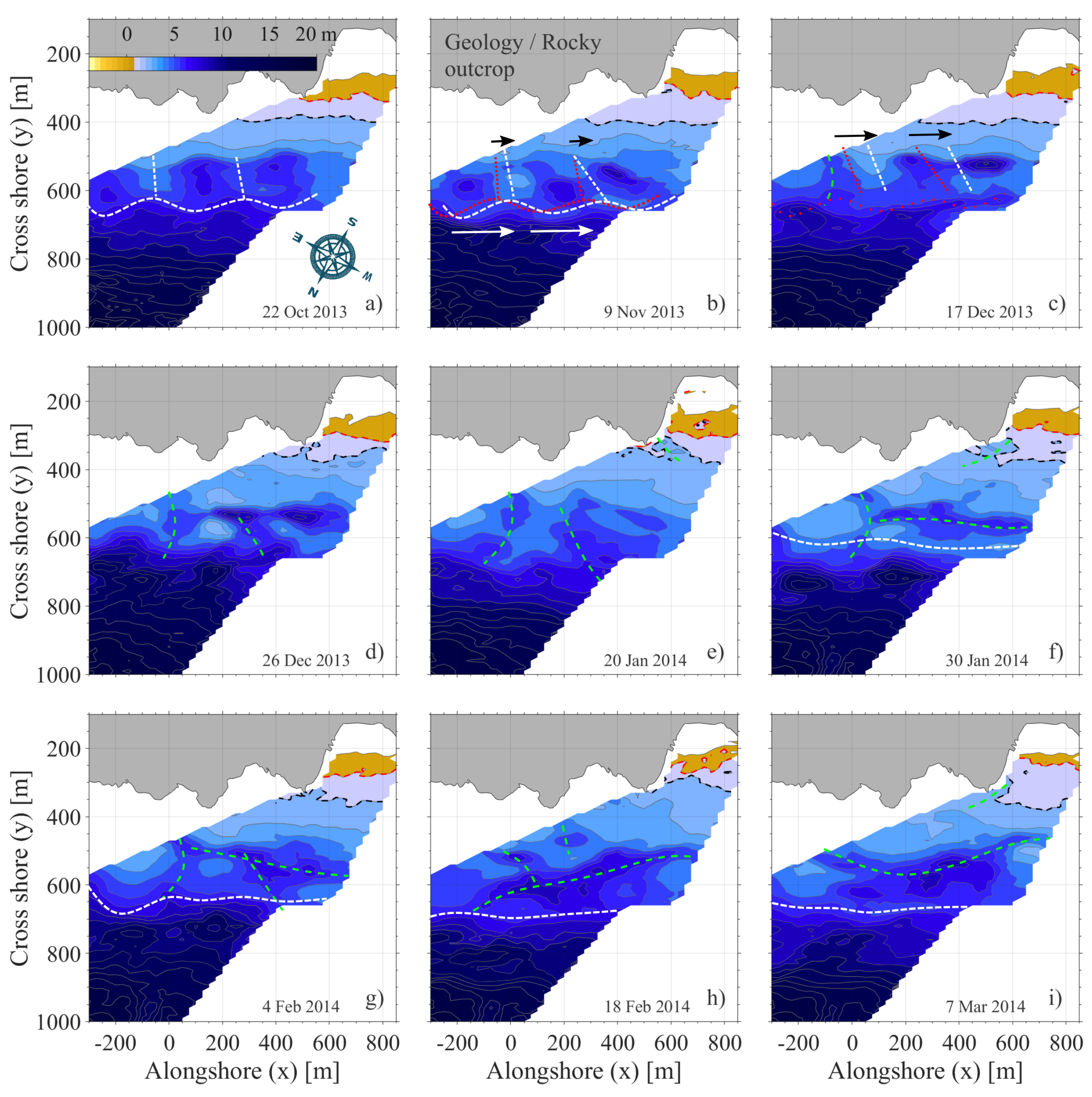
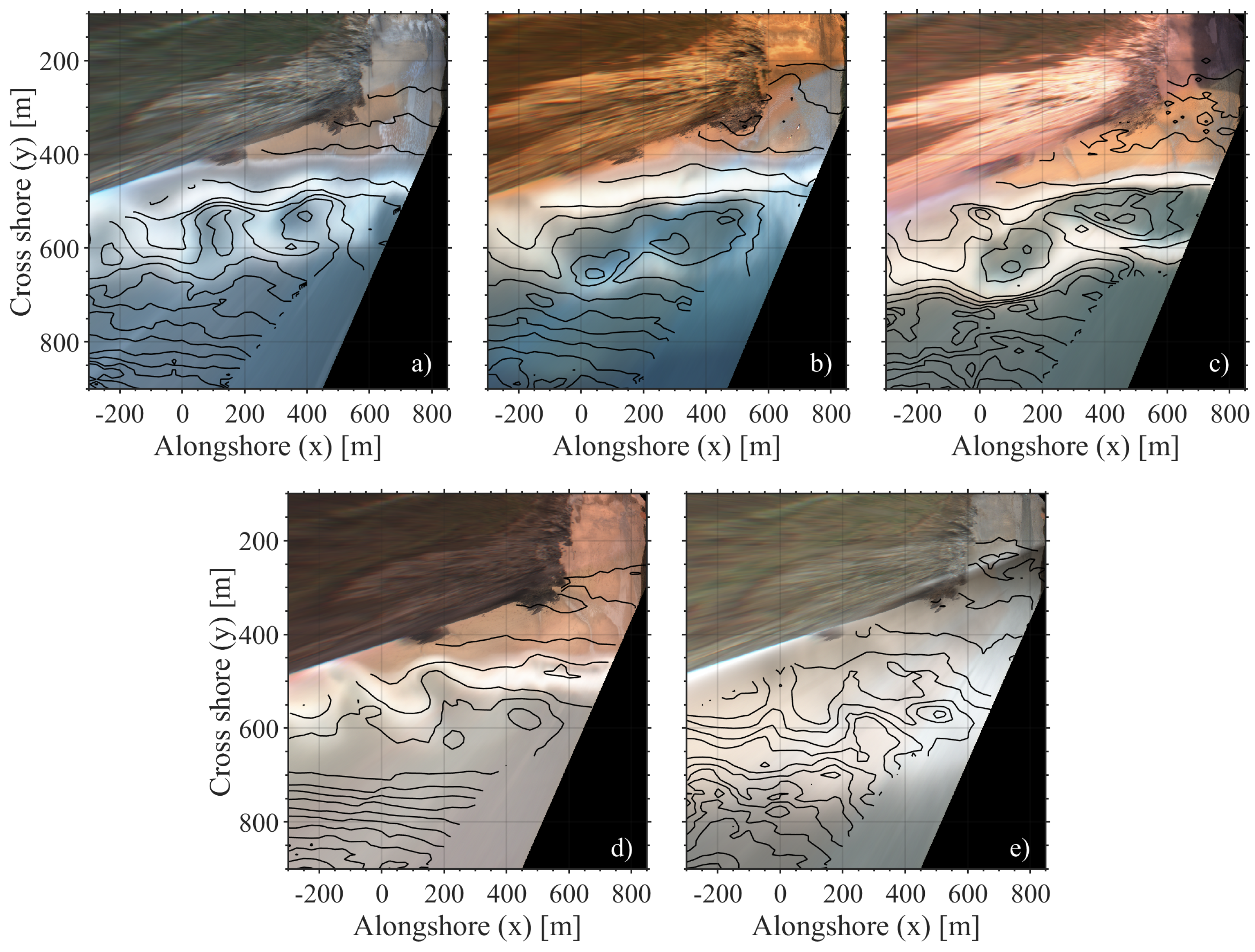
Figure 4a represents the start of the dataset and run chronologically through the extreme 2013–2014 winter. Bathymetries were estimated hourly but here we have selected an arbitrary set of moments in time. Figure 4a is a typical example of a crescentic bar attached to the beach (transverse beach state) [8]. During the first months (October to mid-December) we observe an alongshore migration of the three-dimensional features (indicated by the black and white arrows in Figure 4a–c) and Figure 4c also indicates the formation of a rip channel around m (green dashed line). These large rip channels stayed present throughout Figure 4c–h and it might be that they functioned as a catalyst for inter-tidal beach erosion as observed in [59,60,61]. End-January, a sub-tidal bar seemed more distinct and remained throughout time (white dashed line around 700 m cross-shore (y) in Figure 4f–i). A less powerful storm, but with a greater incident angle, occurred on 5 February 2014 (Table 1). The sub-tidal bar seemed to be significantly more alongshore uniform in Figure 4h. From 4 February to 18 February less powerful storms (compared to 1 February 2014) hit the coast. Figure 4 shows a textbook example of up-state beach changes under erosive conditions, wherein Figure 4a shows a clear transverse bar and beach (TBB) state, and the Figure 4b–i show a rhythmic bar and beach (RBB) to longshore bar-through (LBT) beach state.
3.1.2. Recovery, from Event to Seasonal Scale
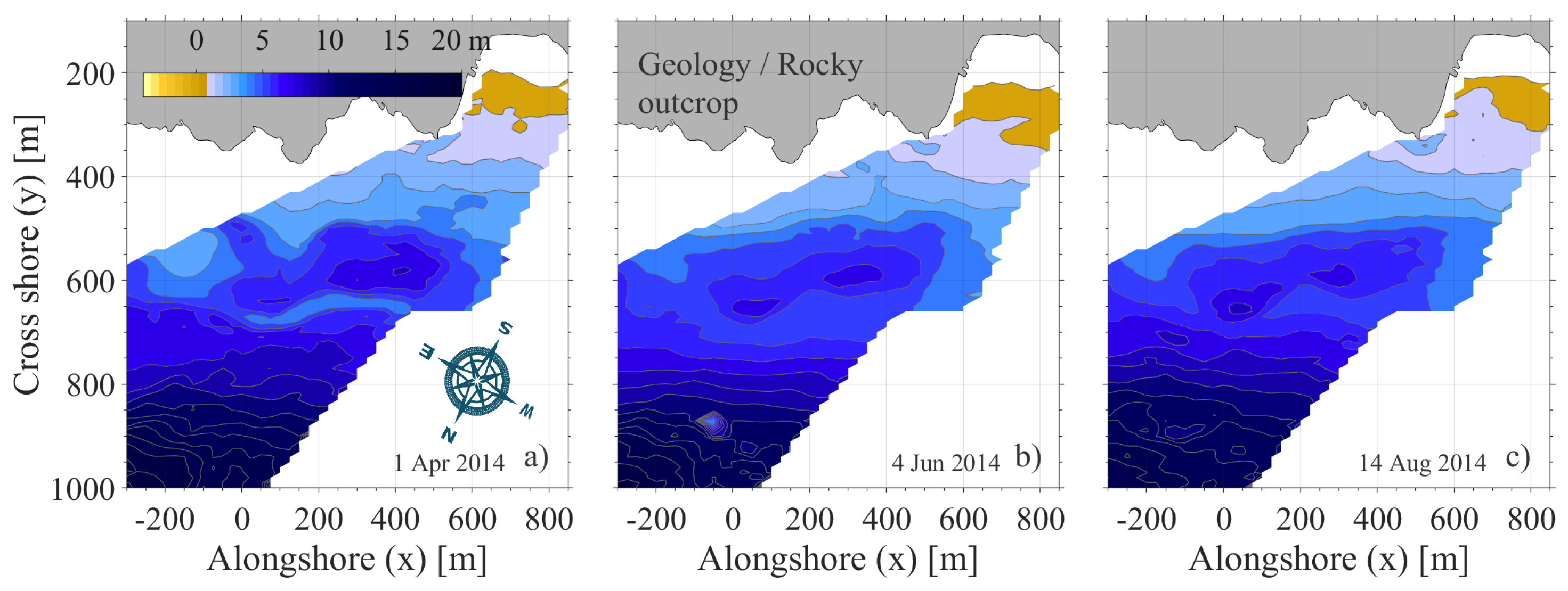
Wave conditions during the summer months were generally less powerful in comparison to the winter months. Hence, morphological change was typically weaker from April to September. From Figure 5 it is apparent that over the summer months large rip channels in the sub-tidal domain ( m) diminish (fill). A persistent rip channel around the main headland remained ( m, m) over the same period, seemingly linked to the local geology. The upper beach face shows some beach erosion in the vicinity of the rocky outcrop (visible in Figure 5c: m, m), presumably linked to the existence of mentioned rip-channel. The cross-shore position of the sub-tidal bar seems to be near-constant as the mean sub-tidal bar position migrates marginally shoreward ( 650 to 625 m).
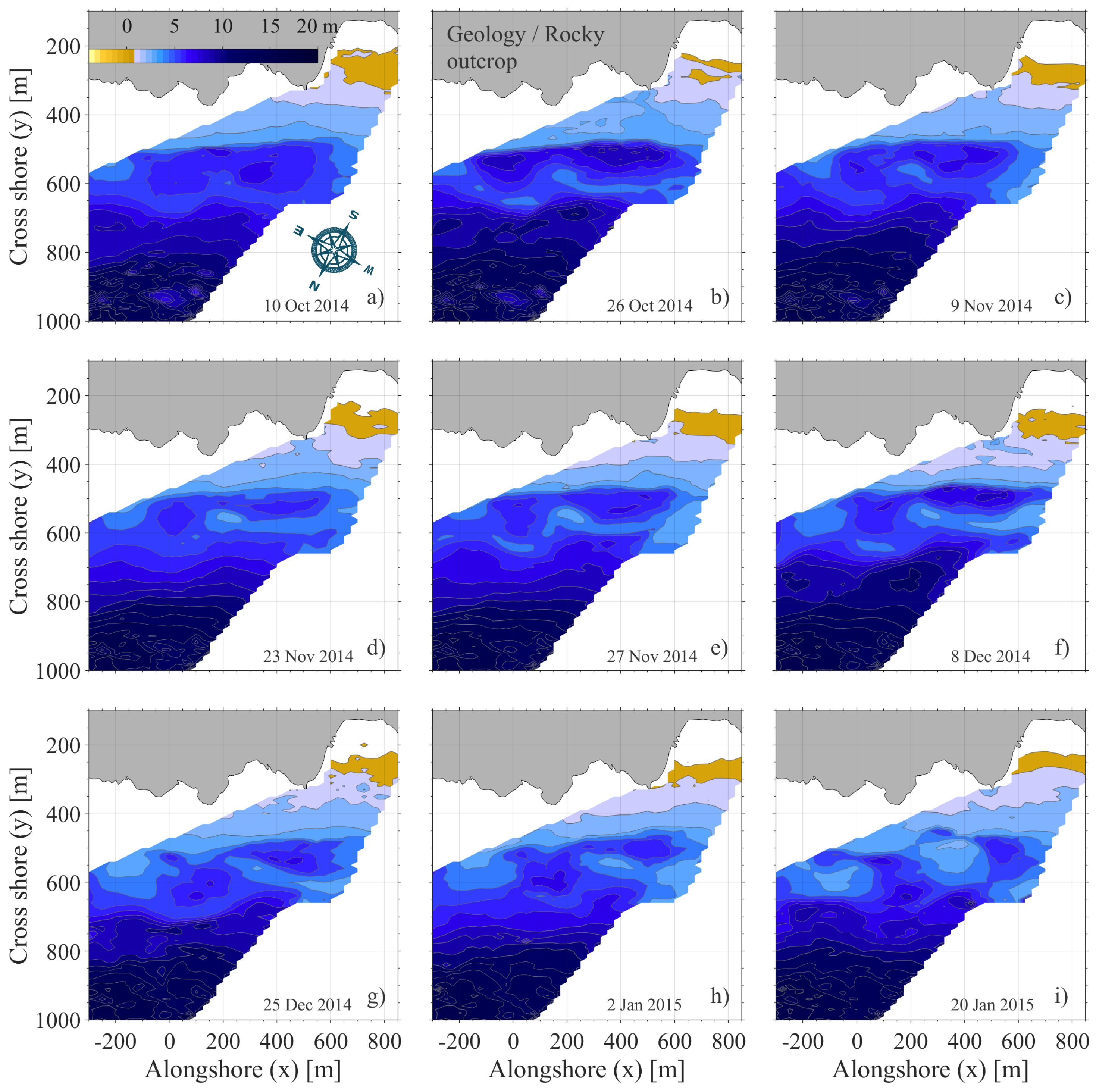
The limited morphological activity remains between August 2014 (Figure 5c) and October 2014 (Figure 6a). The cross-shore position of the sub-tidal bar started to move under increasingly powerful incident waves from October to December 2014. From October to 8 December 2014 (Figure 6a–f) the sub-tidal bar migrated shoreward, becomes more crescentic and partially welds with inter-tidal beach around 200 m. It seems that although the wave conditions were more powerful and beach erosion typically occurred during this period, the shoreward movement of sediments results in inter-tidal beach accretion. Hence further recovery from the occurred erosion in the previous winter occurs during the following fall/winter season. On 10 December 2014, the first storm of the 2014–2015 winter season occurred. Figure 6f represents the bathymetry two days before the first storm of the season. This storm halted the recovery and the relatively more powerful wave conditions caused erosion. The final video-derived bathymetry of the dataset is estimated on 20 January 2015 (Figure 6i)—still during the winter season. The sub-tidal bar distinct crescentic bar welded to the inter-tidal beach and formed a more transverse bar and beach state. At the bar welding position identified above between 200 to 400 m, a large amount of sediment was deposited which shows similarities to a shoreward propagative accretive wave (SPAW) as observed by Wijnberg and Holman [62] and Almar et al. [63].
3.1.3. Cross Shore Bar-Positions
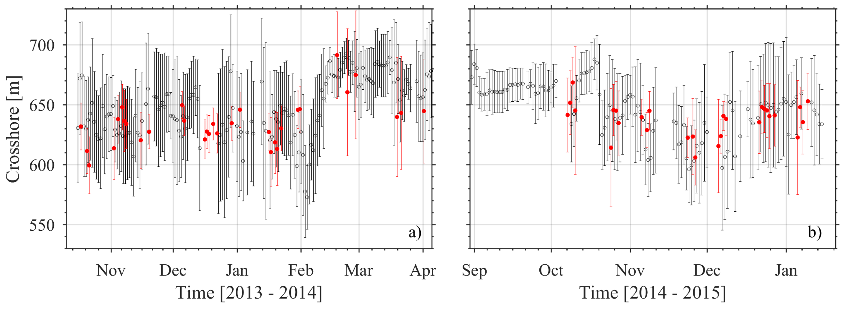
Over the alongshore direction, mean position and standard deviations are computed allowing bar migration and three-dimensionality tracking in time (Figure 7). Mean sub-tidal bar positions and its standard deviation are intrinsically coupled [26]. For example, bar three-dimensionality and hence the standard deviation is bound to increase as a dissipative linear bar migrates shoreward (down-state transition).
Figure 7 follows largely the morphological behaviour as described with the bathymetry estimates in the Results section. The alongshore mean sub-tidal bar position meandered between 600 m and 650 m cross shore from October to December 2013. The sub-tidal bar migrated offshore (between 650 to 700 m) and the three-dimensionality decreased under the extreme storm condition in January/February 2014. From October to December 2014 Figure 7b shows a shoreward migration of the sub-tidal bar coinciding with its increasing three-dimensionality.
3.1.4. Cross Shore Volumetric Change
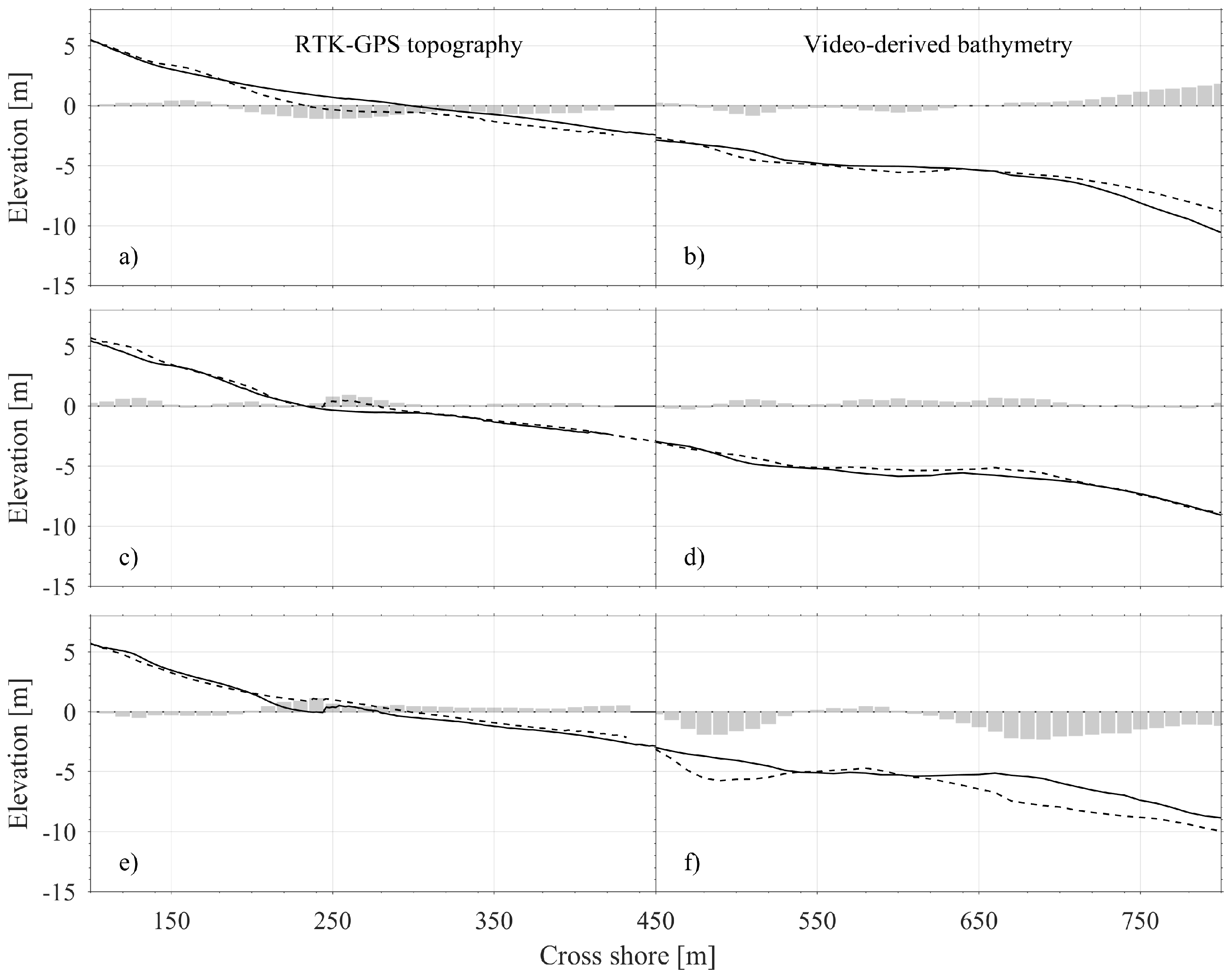
Following Section 2.6, cross-shore profiles were constructed. Cross-shore profiles changed over three periods (winter 2013–2014, summer 2014 and fall 2014–2015) are presented in Figure 8.
The grey bars in Figure 8 indicate the difference per 10 m cross-shore distance over the alongshore average profile. Figure 8 shows that during the first period (Figure 8a,b) the inter-tidal beach lost volume while the sub-tidal domain gained volume. During the summer season of 2014 (Figure 8c,d), the total domain gained volume. During the 2014 fall and part of the 2014 winter season (Figure 8e,f) the inter-tidal beach gained volume (recovery) while the sub-tidal domain lost volume.
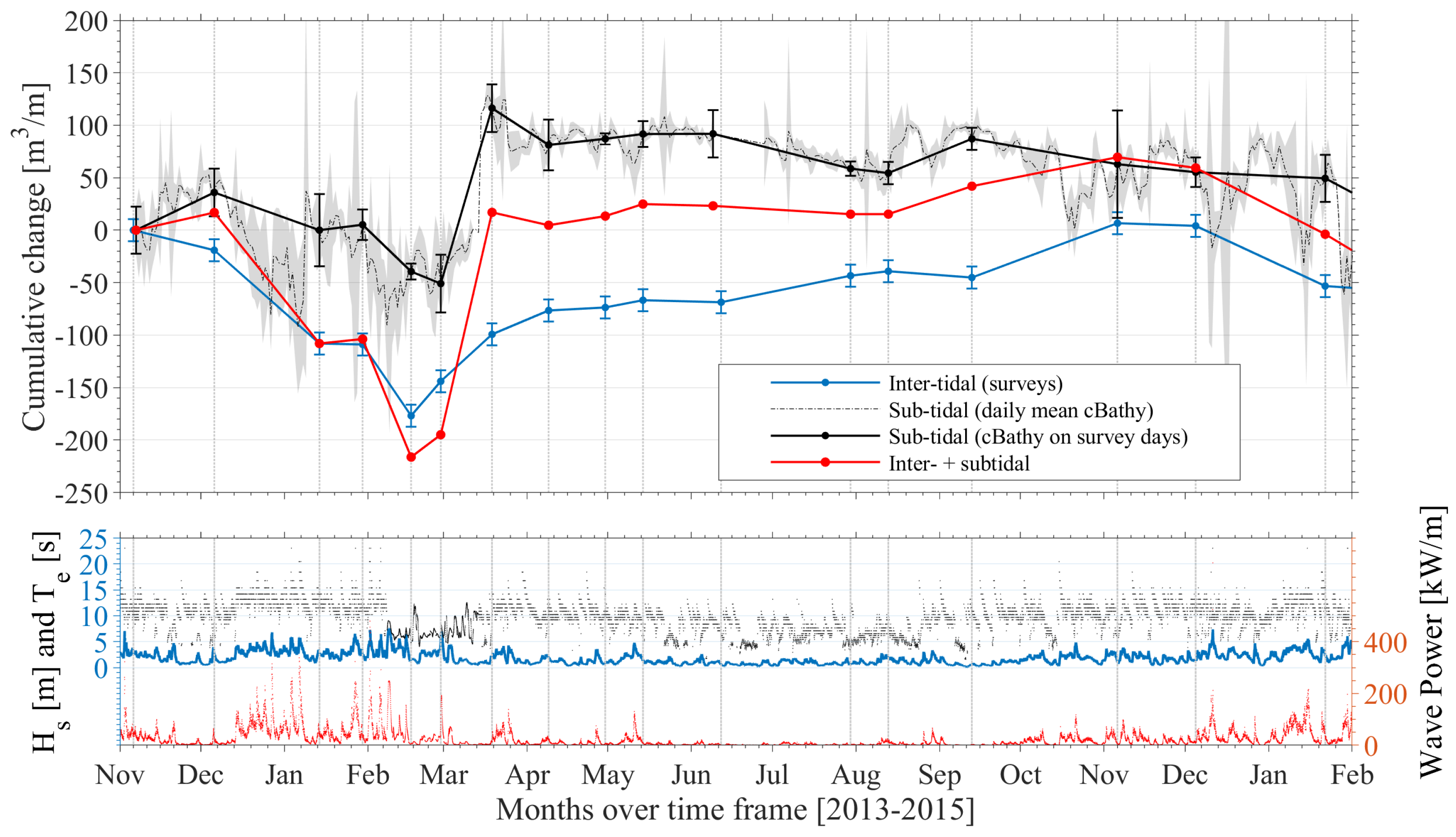
Cumulative volume changes were divided into inter- and sub-tidal zones. Those zones and a combination of the two are depicted in the upper panel of Figure 9. From the start in November 2013 until the peak in storm power in mid-February, the inter-tidal zone eroded. The sub-tidal zone (400–800 m cross-shore) initially gained volume, but as incident wave power increased in early-December 2014, the sub-tidal domain also lost sediment ( m3/m). Over the two months following the most powerful storm (1 February 2014), of the inter-tidal volume is recovered (survey—9 April 2014: +100.4 m3/m—cumulative: m3/m). Sub-tidal zone sediment accumulation over the same time-frame seemed slightly delayed, but the accretion rate significantly greater. Considering the inter- and sub-tidal domain together (red-line in Figure 9) in April 2014 sediment volume levels were back to the level in December 2013. The positive value of the sub-tidal data on the survey days indicates that most of the previously inter-tidal volume was deposited in the sub-tidal domain. During and shortly after the storms, the inter- and sub-tidal domain show comparable cross shore volume change patterns. Over the summer months (June–September; limited incident wave power) the inter- and sub-tidal domain seemed to interact. For example, inter-tidal volume gain coincided with a loss in the sub-tidal domain. A correlation factor of between April and December 2014 further illustrates this inverse behavior. This period highlights slow inter-tidal beach recovery. At the end of the summer (13 September 2014) of the alongshore average inter-tidal beach volume is recovered (+32.4 m3/m cumulative value: m3/m). Full inter-tidal beach recovery was measured during the survey on 6th November 2016. For comparison, of the inter-tidal beach recovery occurred over the summer while more than recovery was achieved during increasingly more powerful wave conditions between September and November 2014 (over a shorter period, thus with a quicker recovery rate). During the latter period, shoreward bar migration was observed, as outlined in previous sections, and this is apparent in cross shore volume exchange between the inter- and sub-tidal area. Yet, the reduced sub-tidal volume did not match the increased inter-tidal domain volume. This suggests that sediment entered the sub-tidal domain from deeper waters during this period.
4. Discussion
4.1. Multi-Scale Morphological Evolution: The Interplay Between an Event and Seasonal Scale
Over the 1.5 year study period, morphological response to similar wave conditions differs significantly. During the 2013–2014 winter season typical upper beach face steepening, lower beach face flattening with inter-tidal beach erosion and offshore storm deposits is observed. The beach state evolves from a Transverse Bar Rip (TBR) state to an LBT following [8]. Considering the straightened sub-tidal sandbars, the 2013–2014 winter can be seen as a morphological reset [17,64]. During extreme storm conditions (2013 winter season), the video-derived bathymetries indicate mega-rips, likewise observed 5 km North [60]. Slow and partial inter-tidal beach recovery occurred during calmer summer conditions while the sub-tidal area develops more and more towards an RBB state. As wave conditions severed during fall and winter season of 2014, inter-tidal beach recovery intensified. While one would expect these more powerful conditions to have an erosive and up-state effect on the beach, the beach state actually evolved down-state into a TBR state; shoreward sub-tidal bar migration leading eventually to bar welding to the beach. More rapid and full recovery (in terms of volume) from the extreme 2013–2014 winter season was achieved between September and December 2014, under typical erosive wave conditions (found at a similar beach configuration 5 km North Davidson et al. [6]). The results of this work show relativism to what higher and lower wave energy means in conceptual morphological models. Antecedent wave conditions determine under what wave conditions recovery occurs. The morphological memory of an extreme winter retains longer and requires wave conditions that are less energetic relative to the extreme that caused the morphological reset, but powerful enough to drive sediment transport, for recovery to occur [6]. In this case, these wave conditions are typically energetic (e.g., conditions that would be erosive after a non-extreme winter) but lead in this case to accretion. During these energetic conditions, onshore migration and slow three-dimensional evolution of the bar coincided with inter-tidal beach recovery.
Initial recovery seems to happen at a different time scales comparing the inter- and sub-tidal zones. A remarkable of the lost inter-tidal volume (RTK-GPS) is recovered within 60 days. Recovery also observed by Coco et al. [17]. The sub-tidal zone shows an even shorter time scale over which it accumulated sediment and gained volume in comparison to the start of the dataset. Although the wave conditions were still energetic during this recovery period, they are relatively calm relative to the preceding extreme wave conditions. Rapid recovery after a storm is consistent with earlier observations and has been linked to a continuous dynamic adaptation to an equilibrium between forcing and beach profile [6,8,17,49,65,66]. Nonetheless, most studies are limited to the inter-tidal domain. The eroded material from the inter-tidal and accreted volume in the sub-tidal do not cancel each other out, meaning that the total near-shore gained volume over this period. On the one hand, extra sediment in the sub-tidal could be a model artifact in the video-derived bathymetries. On the other hand, considering the degree of wave power over the 2013–2014 winter it could be possible that sediment previously stored in deeper waters has been transported from deeper waters into the littoral cell. Significantly larger wave periods have the ability to morphologically activate deeper waters. However, the offshore extent of the video-derived bathymetries is insufficient to confirm this hypothesis.
4.2. Pixel Intensities and Estimated Bathymetries
An evident and eye-catching difference between the red (pixel) and grey (bathymetry estimates) dots in Figure 7 is the different temporal resolution that is obtained between the two techniques. Note that the possibility to determine the beach state from projected images depends on foam visibility. Figure 10a–c highlights the use of projected imagery to determine the beach state. Qualitatively, Figure 10a–c shows that the projected Timex images, especially the foam patterns, follow similar patterns in comparison to quantitative video-derived bathymetries. Nonetheless, foam patterns in the Timex images depend significantly on tidal elevation and incident wave height and period [25]. For instance, on the one hand in the case of “extremely” powerful incident wave conditions, the surf zone width increases to such an extent that pixel intensity saturation occurs in the surf zone. This leads to incorrect identification of the bar position and width or, in case of intensity saturation, it is not possible to identify the bar, as shown in Figure 10e. On the other hand, under calm wave conditions and/or high tidal elevation waves often do not break over the bar and bar detection is not possible. Figure 10d shows the lack of foam patterns over the sub-tidal bar during low-tide due to the calm wave conditions. As a result, in highly energetic macro-tidal environments, such as at Porthtowan beach, determination of the bar position is often only feasible during low-tide and moderate wave conditions. The video-derived bathymetries are less prone to these implications related to environmental forcing. Every hour a bar position can be determined. Note that the video-derived bathymetries are Kalman filtered, and thus smoothed in time.
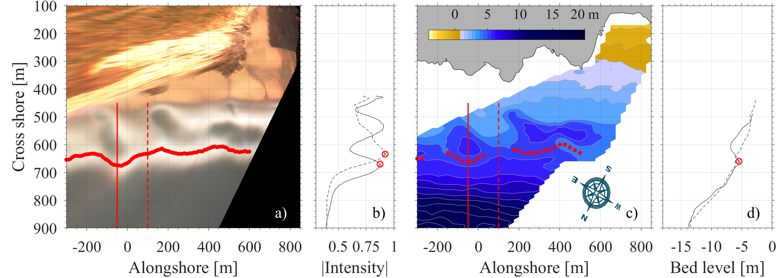
Intensity mapping and associated identification of the bar position is a widely applied approach to monitor sub-tidal bar dynamics [24,25,56,63,67,68,69]. Most of these mentioned applications are in case of the distinct bar features such as alongshore uniform or crescentic bars. As one can imagine, in case of transverse bar/rip configurations, bar detection is more challenging. Results of the bar detection in a transverse bar rip system are presented in Figure 11 using projected pixel intensities and a video-derived bathymetry. The most apparent difference between Figure 11a,c is the alongshore discontinuity of the detected bar position. The discontinuity has mainly to do with the deeper bar crest at those positions. The observed wave-breaking pattern around X = +100 m (red dashed line) using the pixel intensities is detecting a bar while the video-derived bathymetry does not. These continuities (potential false sandbar detections) are also observed in [25,63,67,68,69], in which projected Timex data are further used to analyze sub-tidal bar migration and sandbar three-dimensionality.
4.3. Challenges Related to Depth Inversion Under Extreme Conditions
Environmental conditions are least optimal for the video-derived bathymetries during storm conditions, for example, due to raindrops on the camera lens, reduced visibility, strong winds, large surf zones and messy sea states. Hence, accurate celerity-tracking under these conditions is challenging. During storm conditions, parts of the Kalman filtered video-derived bathymetry become messy and clearly non-physical [37], particularly the inter-tidal zone (hence we use the RTK-GPS measurements for the inter-tidal zone). This happens partially because we allow the bathymetry to change through a process variability function in the Kalman filter [34]. The process variability expression in Holman et al. [34] intrinsically results in greater faith deterioration of the previous estimate under energetic conditions in comparison to calm conditions. In morphological terms, more morphological change can be expected and is numerically allowed during larger wave heights. Bathymetry stabilization occurs as soon as the wave conditions reduce. Wave conditions are relatively calm but still energetic compared to earlier tests [34].
Holman et al. [34] showed a correlation between increasing wave conditions (up to just over 2 m) and RMS error: as wave conditions intensify cBathy tends to increasingly overestimate depth. Finite amplitude dispersion effects are a first-order contribution to these correlations. However, consideration of the accuracy versus wave height requires more context. More energetic wave conditions have positive and negative effects. A positive effect is that under more energetic conditions depths can be estimated in deeper water. Holman et al. [34] and Rutten et al. [36] both show an underestimation bias in deeper water which is respectively linked to a single low-resolution camera and quality control. The former is linked to larger pixel-footprints offshore, wave crests are not recognisable or less distinctive. The same is found for the video-station at Porthtowan limiting the volume analysis domain ( 800 m) to eliminate the deep-water issue for having an effect on the volume analysis. Both test cases are in wind–sea environments with limited wave periods. At Porthtowan, the offshore looking camera also has a limited resolution (1.4 MegaPixels) but the wave period reaches up to 18 s during energetic incident wave conditions. Consequently, the most accurate deeper water estimates are typically estimated during the more energetic conditions. The deep-water estimates remain over time through the Kalman filter assimilation due to relatively low Kalman gain and process variance in deeper water. On the negative side, we find, for example, finite amplitude dispersion [20] and fewer details (relatively small morphological features (in comparison to the wavelength) are not influencing wave pattern) due to greater wave periods. Under more energetic conditions a larger cross shore domain suffers overestimation of the depth due to the amplitude dispersion. Depending on the tidal elevation this has a smaller (large tidal range) or larger (small tidal range) effect. Large tidal ranges such as at Porthtowan (maximum m) compensate partially for the amplitude dispersion as during high-tide wave transformation shifts landward so that theoretically accurate depths are obtained over a larger domain in comparison to small tidal ranges. For the volume analysis in this paper, video derived bathymetries are only used over the sub-tidal area, and RTK-GPS measured topographies for the inter-tidal zone. By limiting the video-derived bathymetry domain to its optimal zones [39], we eliminate the amplitude dispersion effect in our data and hence the volumetric analysis. In addition to amplitude dispersion, the local geology induces local circulation, that is typically responsible for beach rotation and rip channels [59]. It is interesting to note that the video-derived bathymetries in Figure 4 show numerous rip channels seemingly related to the position of the rocky outcrop. These embayed cellular rip channels [61] indicate the existence of rip currents related to the rip channel position and bay circulation. This questions the validity to neglect the most right-hand term in Equation (3) and therefore the necessity to take into account the Doppler effect on incident waves. Lastly, waves refract differently over local bathymetry depending on the wave period and hence allow more detailed bathymetries to be obtained with shorter period waves and vice versa. Large wave periods during the storms have the tendency to spatially smooth the video-derived bathymetry, which results in a more alongshore uniform bathymetry than reality.
5. Conclusions
Here, the first long-term (1.5 years) high spatiotemporal resolution video-derived bathymetry dataset is presented. This video-derived dataset is combined with punctual RTK-GPS measurements of the intertidal beach. The combined dataset allowed for a morphological assessment covering the inter- and sub-tidal domain over short (hours to days) and long (months) time-scales. Beach (state) change is described using the video-derived bathymetries and in terms of cross-shore bar position and volumetric analysis. This work shows the capability of near-continuous monitoring independent from, for example, the visibility of wave-breaking patterns (as in bar detection through pixel intensities). We demonstrate that video-based bathymetry estimates enrich existing intermittent beach measurement as well as opening up the possibility to monitor beach morphology dynamic in between storms. Beach response to storms was formerly impossible to observe using video camera systems due to pixel intensity saturation. The video-derived bathymetries are shown to be effective in determining bar-positions, bar three-dimensionality and volume analyses with an unprecedented hourly temporal resolution (Kalman filtered).
The video-derived dataset indicates that over the extreme 2013–2014 winter season, the pre-existing transverse bar and beach state altered up-state to a straightened longshore bar through beach state. Simultaneously, the inter-tidal beach suffered large erosion. More than half of the eroded material over this period was recovered in the inter-tidal zone within two months after the last major storm. Limited recovery is observed during the summer season () while as soon as wave conditions intensified in fall 2014 inter-tidal beach recovery accelerated. The sub-tidal bar migrated shoreward under typically erosive conditions and the beach state evolved down-state (thus accretive wave conditions) to rhythmic bar and beach and eventually transverse bar and beach state. Full recovery of inter-tidal beach volumes was achieved 9 months after the last extreme storm of the preceding 2013–2014 winter.
Author Contributions
Conceptualization, E.W.J.B., D.C.C., M.A.D. and T.J.O.; methodology, E.W.J.B., D.C.C., M.A.D. and T.J.O.; validation: E.W.J.B., D.C.C., M.A.D., T.J.O. and R.A.; formal analysis: E.W.J.B. writing—original draft preparation: E.W.J.B., D.C.C., M.A.D., T.J.O. and R.A.; writing—review and editing: E.W.J.B., D.C.C., M.A.D., T.J.O. and R.A. visualization: E.W.J.B.; supervision: E.W.J.B., D.C.C., M.A.D. and T.J.O.
Funding
Erwin Bergsma is currently funded by Centre National d’Etudes Spatiales (CNES). Rafael Almar was funded by the French ANR grant (COASTVAR: ANR-14-ASTR-0019).
Acknowledgments
Wave data is acquired from the Channel Coastal Observatory website [http://www.channelcoast.org/]. We would like to greatly thank the reviewers, in particular reviewer-3, for their contribution to improving this manuscript.
Conflicts of Interest
The funders had no role in the design of the study; in the collection, analyses, or interpretation of data; in the writing of the manuscript, or in the decision to publish the results.
Appendix A. Wave Statistics 2008–2017
Wave statistics derived from the wave buoy described in the methods section. Table A1 shows yearly wave statistics over the total data from the 1 of October 2008 until 31 October 2017. In Table A2, wave statistics are presented per winter/summer season. For the analysis here winter is defined as November until March (including) the next year and summer runs from April to September (included).

Table A1.
Yearly wave statistics from 2008–2017. represents the significant wave height. The corresponding peak period and wave direction are respectively indicated by and . P is the instantaneous wave power in kW/m and P is the accumulative hourly wave power over the indicated time frame in MW/m. We present mean values which are denoted with ¯± the standard deviation .
| Period | [m] | [s] | [°] | [kW/m] | ΣP [MW/m] |
|---|---|---|---|---|---|
| 2008–2017 | 1.57 ± 0.94 | 10.51 ± 3.07 | 283.4 ± 26.7 | 17.48 ± 25.84 | 1360.2 |
| 2008 * | 1.94 ± 0.87 | 10.75 ±3.03 | 290.7 ±24.6 | 22.69 ±24.40 | 50.05 |
| 2009 | 1.62 ± 0.96 | 10.84 ± 2.89 | 281.9 ± 51.9 | 19.16 ± 27.15 | 159.86 |
| 2010 | 1.27 ± 0.69 | 10.05 ± 3.27 | 286.1 ± 27.5 | 10.16 ± 15.56 | 88.79 |
| 2011 | 1.66 ± 0.90 | 10.96 ± 3.02 | 281.4 ± 16.4 | 19.12 ± 24.28 | 166.87 |
| 2012 | 1.52 ± 0.86 | 9.98 ± 2.95 | 282.6 ± 21.7 | 14.89 ± 20.50 | 128.10 |
| 2013 | 1.55 ± 0.97 | 10.51 ± 3.09 | 283.0 ± 20.3 | 17.91 ± 27.77 | 153.15 |
| 2014 | 1.65 ± 1.12 | 10.70 ± 3.13 | 284.3 ± 20.2 | 20.10 ± 33.78 | 175.26 |
| 2015 | 1.70 ± 1.01 | 10.59 ± 3.10 | 283.9 ± 20.7 | 20.87 ± 27.83 | 180.64 |
| 2016 | 1.58 ± 0.96 | 10.69 ± 2.99 | 283.1 ± 20.8 | 18.31 ± 28.02 | 160.63 |
| 2017 * | 1.50 ± 0.86 | 10.15 ± 3.05 | 281.5 ± 19.6 | 14.95 ± 20.09 | 96.92 |
* The data used here runs from 1 October 2008 until 31 October 2017.
Table A2.
Seasonal (winter–summer) wave statistics from 2008–2017. The same notations have been used as in Table A1. The grey-highlighted rows illustrates the morphological time-frame coverage.
Table A2.
Seasonal (winter–summer) wave statistics from 2008–2017. The same notations have been used as in Table A1. The grey-highlighted rows illustrates the morphological time-frame coverage.
| Period | [m] | [s] | [°] | [kW/m] | ΣP [MW/m] |
|---|---|---|---|---|---|
| 2008–2017 winter | 1.90 ± 1.04 | 11.71 ± 3.00 | 285.3 ± 31.7 | 25.94 ± 32.19 | 1004.4 |
| 2008–2017 summer | 1.24 ± 0.68 | 9.33 ± 2.66 | 281.7 ± 20.7 | 9.10 ± 12.71 | 355.8 |
| 2008–2009 winter | 1.92 ± 0.93 | 11.61 ± 3.07 | 287.9 ± 24.5 | 24.97 ± 28.72 | 103.95 |
| 2009 summer | 1.30 ± 0.70 | 9.78 ± 2.33 | 281.4 ± 20.6 | 10.25 ± 12.35 | 42.88 |
| 2009–2010 winter | 1.68 ± 1.01 | 11.41 ± 3.28 | 284.5 ± 25.3 | 20.84 ± 28.89 | 90.95 |
| 2010 summer | 1.13 ± 0.50 | 9.21 ± 2.78 | 284.4 ± 23.2 | 6.78 ± 7.54 | 29.78 |
| 2010–2011 winter | 1.53 ± 0.91 | 11.49 ± 3.35 | 287.0 ± 27.4 | 18.36 ± 25.61 | 79.67 |
| 2011 summer | 1.43 ± 0.74 | 9.84 ± 2.69 | 279.8 ± 16.3 | 12.21 ± 15.55 | 53.49 |
| 2011–2012 winter | 1.93 ± 0.94 | 11.46 ± 2.87 | 283.4 ± 16.1 | 24.90 ± 28.12 | 105.92 |
| 2012 summer | 1.22 ± 0.70 | 8.79 ± 2.39 | 280.2 ± 22.4 | 8.45 ± 13.89 | 36.87 |
| 2012–2013 winter | 1.79 ± 0.96 | 11.42 ± 3.11 | 284.5 ± 23.2 | 21.97 ± 25.23 | 94.84 |
| 2013 summer | 1.23 ± 0.71 | 9.26 ± 2.62 | 281.3 ± 18.1 | 9.19 ± 13.93 | 38.93 |
| 2013–2014 winter | 2.30 ± 1.28 | 12.36 ± 2.82 | 287.0 ± 17.7 | 37.72 ± 47.02 | 163.17 |
| 2014 summer | 1.05 ± 0.60 | 9.15 ± 2.75 | 282.7 ± 22.5 | 6.42 ± 10.01 | 28.11 |
| 2014–2015 winter | 2.12 ± 1.03 | 11.87 ± 2.63 | 284.8 ± 18.7 | 30.74 ± 32.77 | 133.25 |
| 2015 summer | 1.26 ± 0.66 | 9.24 ± 2.78 | 283.0 ± 22.8 | 8.94 ± 11.45 | 39.20 |
| 2015–2016 winter | 2.16 ± 1.11 | 12.02 ± 2.76 | 283.3 ± 17.3 | 33.73 ± 37.58 | 145.54 |
| 2016 summer | 1.28 ± 0.68 | 9.42 ± 2.69 | 280.6 ± 19.1 | 9.75 ± 12.37 | 42.80 |
| 2016–2017 winter | 1.69 ± 0.92 | 11.72 ± 2.94 | 284.7 ± 24.5 | 20.25 ± 22.79 | 86.77 |
| 2017 summer | 1.29 ± 0.74 | 9.27 ± 2.65 | 280.6 ± 8.16 | 9.99 ± 14.42 | 43.75 |
Appendix B. cBathy Applications
In this Appendix, we present previous studies using cBathy to highlight their location, duration, and the number of samples. Specific cases are further discussed in terms of, for example, accuracy in the manuscript.
Table A3.
Previous cBathy applications. Abbreviations for the Frequency column: single: single estimate, intermittent: int. and full: a bathymetry every for all possible collections (at Porthtowan this means hourly). For the Type column the abbreviations are, Validation: Val., Volume analysis: Vol., Bar tracking: bar and Beach state analysis: BS.
| Period | Reference | Location | Frequency | #-obs | Type | Wave Cond. | Tide |
|---|---|---|---|---|---|---|---|
| 2009–2011 | Holman et al. [34] | Duck, NC USA | int. | 16 | Val. | calm/storm | micro |
| June 2013–March 2014 | Rutten et al. [36] | Sand Engine, The Netherlands | int. | 6 | Vol. | calm | micro |
| 13 July 2013 | Holman et al. [34] | Agate Beach, OR, USA | single | 1 | Val. | calm | meso |
| 17 May 2012 | Holman and Stanley [70] | New River Inlet, NC, USA | single | 1 | Val. | calm | micro |
| 10–17 April 2014 * | Bergsma et al. [35] | Porthtowan, Cornwall, UK | int. | 2 | Val. | calm | macro |
| 17–20 February 2013 | Wengrove et al. [71] | Kijkduin, The Netherlands | int. | 2 | Val. | calm | micro |
| 1–4 July 2013 | Radermacher et al. [72] | Sand Engine, The Netherlands | single | 1 | Val. | calm | micro |
| September 2015–September 2016 | Brodie et al. [37] | Duck, NC USA | full/int. | full/6 | Val./bar | calm/storm | micro |
| October 2013–February 2014 * | this study | Porthtowan, Cornwall, UK | full/int. | full/21 | BS, bar, Vol. | calm/storm | macro |
* cBathy adapted for large tidal ranges.
References
- Melet, A.; Meyssignac, B.; Almar, R.; Cozannet, G.L. Under-estimated wave contribution to coastal sea-level rise. Nat. Clim. Chang. 2018, 8, 234–239. [Google Scholar] [CrossRef]
- Dodet, G.; Bertin, X.; Taborda, R. Wave climate variability in the North-East Atlantic Ocean over the last six decades. Ocean Model. 2010, 31, 120–131. [Google Scholar] [CrossRef]
- Lazarus, E.D.; Ellis, M.A.; Murray, A.B.; Hall, D.M. An evolving research agenda for human-coastal systems. Geomorphology 2016, 256, 81–90. [Google Scholar] [CrossRef]
- Wang, X.L.; Feng, Y.; Swail, V.R. North Atlantic wave height trends as reconstructed from the 20th century reanalysis. Geophys. Res. Lett. 2012, 39, 1–6. [Google Scholar] [CrossRef]
- Woolf, D.; Wolf, J. Impacts of climate change on storms and waves. MCCIP Sci. Rev. 2013, 20–26. [Google Scholar] [CrossRef]
- Davidson, M.A.; Splinter, K.D.; Turner, I.L. A simple equilibrium model for predicting shoreline change. Coast. Eng. 2013, 73, 191–202. [Google Scholar] [CrossRef]
- Phillips, M.S.; Harley, M.D.; Turner, I.L.; Splinter, K.D.; Cox, R.J. Shoreline recovery on wave-dominated sandy coastlines: The role of sandbar morphodynamics and nearshore wave parameters. Mar. Geol. 2017, 385, 146–159. [Google Scholar] [CrossRef]
- Wright, L.; Short, A.D. Morphodynamic variability of surf zones and Beaches; A Synthesis. Mar. Geol. 1984, 56, 93–118. [Google Scholar] [CrossRef]
- Almar, R.; Marchesiello, P.; Almeida, L.P.; Thuan, D.H.; Tanaka, H.; Viet, N.T. Shoreline Response to a Sequence of Typhoon and Monsoon Events. Water 2017, 9, 364. [Google Scholar] [CrossRef]
- Martins, K.; Blenkinsopp, C.E.; Zang, J. Monitoring Individual Wave Characteristics in the Inner Surf with a 2-Dimensional Laser Scanner (LiDAR). J. Sens. 2016, 2016, 7965431. [Google Scholar] [CrossRef]
- Martins, K.; Blenkinsopp, C.E.; Power, H.E.; Bruder, B.; Puleo, J.A.; Bergsma, E.W.J. High-resolution monitoring of wave transformation in the surf zone using a LiDAR scanner array. Coast. Eng. 2017, 128, 37–43. [Google Scholar] [CrossRef]
- Larson, M.; Kraus, N.C. Temporal and spatial scales of beach profile change, Duck, North Carolina. Mar. Geol. 1994, 117, 75–94. [Google Scholar] [CrossRef]
- Birkemeier, W.A.; Baron, C.F.; Leffier, M.W.; Miller, H.C.; Strider, J.B.; Hathawa, K.K. SUPERDUCK Nearshore Processes Experiment: Data Summary, Miscellaneous Report; Technical Report; US Army Corps of Engineers: Washington, DC, USA, 1989.
- Sénéchal, N.; Gouriou, T.; Castelle, B.; Parisot, J.; Capo, S.; Bujan, S.; Howa, H. Morphodynamic response of a meso- to macro-tidal intermediate beach based on a long-term data set. Geomorphology 2009, 107, 263–274. [Google Scholar] [CrossRef] [Green Version]
- Harley, M.D.; Turner, I.L.; Short, A.D.; Ranasinghe, R. Assessment and integration of conventional, RTK-GPS and image-derived beach survey methods for daily to decadal coastal monitoring. Coast. Eng. 2011, 58, 194–205. [Google Scholar] [CrossRef]
- Poate, T.; Masselink, G.; Russell, P.; Austin, M. Morphodynamic variability of high-energy macrotidal beaches, Cornwall, UK. Mar. Geol. 2014, 350, 97–111. [Google Scholar] [CrossRef] [Green Version]
- Coco, G.; Sénechal, N.; Rejas, A.; Bryan, K.; Capo, S.; Parisot, J.; Brown, J.; MacMahan, J. Beach response to a sequence of extreme storms. Geomorphology 2014, 204, 493–501. [Google Scholar] [CrossRef] [Green Version]
- Masselink, G.; Scott, T.; Poate, T.; Russell, P.; Davidson, M.; Conley, D. The extreme 2013/2014 winter storms: Hydrodynamic forcing and coastal response along the southwest coast of England. Earth Surf. Process. Landf. 2015, 41, 378–391. [Google Scholar] [CrossRef]
- Ranasinghe, R.; Callaghan, D.; Roelvink, D. Does a more sophisticated storm erosion model improve probabilistic erosion estimates? In Proceedings of the 7th International Conference on Coastal Dynamics, Arcachon, France, 24–28 June 2013. [Google Scholar]
- Bergsma, E.W.J.; Almar, R. Video-based depth inversion techniques, a method comparison with synthetic cases. Coast. Eng. 2018, 138, 199–209. [Google Scholar] [CrossRef]
- Wilson, G.; Özkan-Haller, H.; Holman, R. Data assimilation and bathymetric inversion in a two-dimensional horizontal surf zone model. J. Geophys. Res. 2010, 115. [Google Scholar] [CrossRef] [Green Version]
- Wilson, G.; Özkan-Haller, H.; Holman, R.; Haller, M.; Honegger, D.; Chickadel, C. Surf zone bathymetry and circulation predictions via data assimilation of remote sensing observations. J. Geophys. Res. Oceans 2014. [Google Scholar] [CrossRef]
- Ludeno, G.; Reale, F.; Dentale, F.; Carratelli, E.P.; Natale, A.; Serafino, F. Estimating Nearshore Bathymetry from X-Band Radar Data. Coast. Ocean Obs. Syst. 2015, 265–280. [Google Scholar] [CrossRef]
- Plant, N.G.; Holman, R.A.; Freilich, M. A simple model for interannual sandbar behavior. J. Geophys. Res. 1999, 104, 15755–15776. [Google Scholar] [CrossRef] [Green Version]
- Van Enckevort, I.; Ruessink, B. Effect of Hydrodynamics and bathymetry on video estimates of nearshore sandbar position. J. Geophys. Res. 2001, 106, 16969–16979. [Google Scholar] [CrossRef]
- Plant, N.G.; Holland, K.T.; Holman, R.A. A dynamical attractor governs beach response to storms. Geophys. Res. Lett. 2006, 33, 1–6. [Google Scholar] [CrossRef]
- Price, T.; Ruessink, B. State Dynamics of a double sandbar system. Cont. Shelf Res. 2011, 31, 659–674. [Google Scholar] [CrossRef]
- Grilli, S.T. Depth inversion in shallow water based on nonlinear properties of shoaling periodic waves. Coast. Eng. 1998, 35, 185–209. [Google Scholar] [CrossRef] [Green Version]
- Bell, P.S. Shallow water bathymetry derived from an analysis of X-band marine radar images of waves. Coast. Eng. 1999, 37, 513–527. [Google Scholar] [CrossRef]
- Stockdon, H.F.; Holman, R.A. Estimation of wave phase speed and nearshore bathymetry from video imagery. J. Geophys. Res. 2000, 105, 22015–22033. [Google Scholar] [CrossRef] [Green Version]
- Senet, C.M.; Seemann, J.; Flampouris, S.; Ziemer, F. Determination of Bathymetric and Current Maps by the Method DiSC Based on the Analysis of Nautical X-Band Radar Image Sequences of the Sea Surface (November 2007). IEEE Trans. Geosci. Remote Sens. 2008, 46, 2267–2279. [Google Scholar] [CrossRef]
- Almar, R.; Bonneton, P.; Senechal, N.; Roelvink, D. Wave Celerity From Video Imaging: A new method. In Proceedings of the 31st International Conference Coastal Engineering, Hamburg, Germany, 31 August–5 September 2008; pp. 1–14. [Google Scholar]
- Plant, N.G.; Holland, K.T.; Haller, M.C. Ocean Wavenumber Estimation From Wave-Resolving Time Series Imagery. IEEE Trans. Geosci. Remote Sens. 2008, 46, 2644–2658. [Google Scholar] [CrossRef]
- Holman, R.A.; Plant, N.; Holland, T. cBathy: A Robust Algorithm For Estimating Nearshore Bathymetry. J. Geophys. Res. Oceans 2013, 118, 2595–2609. [Google Scholar] [CrossRef]
- Bergsma, E.W.J.; Conley, D.C.; Davidson, M.A.; O’Hare, T.J. Video-Based Nearshore Bathymetry Estimation in Macro-Tidal Environments. Mar. Geol. 2016, 374, 31–41. [Google Scholar] [CrossRef]
- Rutten, J.; de Jong, S.M.; Ruessink, G. Accuracy of Nearshore Bathymetry Inverted From X-Band Radar and Optical Video Data. IEEE Trans. Geosci. Remote Sens. 2017, 55, 1106–1116. [Google Scholar] [CrossRef]
- Brodie, K.L.; Palmsten, M.L.; Hesser, T.J.; Dickhudt, P.J.; Raubenheimer, B.; Ladner, H.; Elgar, S. Evaluation of video-based linear depth inversion performance and applications using altimeters and hydrographic surveys in a wide range of environmental conditions. Coast. Eng. 2018, 136, 147–160. [Google Scholar] [CrossRef] [Green Version]
- Sembiring, L.; van Dongeren, A.; Winter, G.; van Ormondt, M.; Briere, C.; Roelvink, D. Nearshore bathymetry from video and the application to rip current predictions for the Dutch Coast. J. Coast. Res. 2014, 70, 354–359. [Google Scholar] [CrossRef]
- Bergsma, E.W.J. Application of an Improved Video Based Depth Inversion Technique to A Macrotidal Sandy Beach. Ph.D. Thesis, Plymouth University, CPRG, Plymouth, UK, 2017. [Google Scholar]
- Buscombe, D.; Scott, T. Coastal Geomorphology of North Cornwall: St Ives to Trevose Head. Internal Report for Wave Hub Impacts on Seabed and Shoreline Processes; Technical Report; University of Plymouth: Plymouth, UK, 2008. [Google Scholar]
- Scott, T.; Masselink, G.; Russell, P. Morphodynamic characteristics and classification of beaches in England and Wales. Mar. Geol. 2011, 286, 1–20. [Google Scholar] [CrossRef] [Green Version]
- Holman, R.; Stanley, J. The history and technical capabilities of Argus. Coast. Eng. 2007, 54, 477–491. [Google Scholar] [CrossRef]
- Cahill, B.; Lewis, T. Wave period ratios and the calculation of wave power. In Proceedings of the 2nd Marine Energy Technology Symposium, Seattle, WA, USA, 15–17 April 2014; pp. 1–10. [Google Scholar]
- Leffler, K.E.; Jay, D.A. Enhancing tidal harmonic analysis: Robust (hybrid L1/L2) solutions. Cont. Shelf Res. 2009, 29, 78–88. [Google Scholar] [CrossRef]
- Morton, R.A.; Gibeaut, J.C.; Paine, J.G. Meso-scale transfer of sand during and after storms: Implications for prediction of shoreline movement. Mar. Geol. 1995, 126, 161–179. [Google Scholar] [CrossRef]
- Ferreira, O. Storm groups versus extreme single storms: Predicted erosion and management consequences. J. Coast. Res. 2005, 42, 221–227. [Google Scholar]
- Masselink, G.; Castelle, B.; Scott, T.; Dodet, G.; Suanez, S.; Jackson, D.; Floc’h, F. Extreme wave activity during 2013/2014 winter and morphological impacts along the Atlantic coast of Europe. Geophys. Res. Lett. 2016, 43, 2135–2143. [Google Scholar] [CrossRef] [Green Version]
- Harley, M.D.; Turner, I.L.; Short, A.D.; Ranasinghe, R. An empirical model of beach response to storms-SE Australia. In Proceedings of the 19th Australasian Conference on Coastal and Ocean Engineering, Wellington, New Zealand, 16–18 September 2009. [Google Scholar]
- Splinter, K.D.; Carley, J.T.; Golshani, A.; Tomlinson, R. A relationship to describe the cumulative impact of storm clusters on beach erosion. Coast. Eng. 2014, 83, 49–55. [Google Scholar] [CrossRef]
- Castelle, B.; Marieu, V.; Bujana, S.; Splinter, K.D.; Robinet, A.; Sénechal, N.; Ferreira, S. Impact of the winter 2013–2014 series of severe Western Europe storms on a double-barred sandy coast: Beach and dune erosion and megacusp embayments. Geomorphology 2015, 238, 135–148. [Google Scholar] [CrossRef]
- Merrifield, M.A.; Guza, R.T. Detecting Propagating Signals with Complex Empirical Orthogonal Functions: A Cautionary Note. J. Phys. Oceanogr. 1990, 20, 1628–1633. [Google Scholar] [CrossRef] [Green Version]
- Holland, T.K. Application of the Linear Dispersion Relation with Respect to Depth Inversion and Remotely Sensed Imagery. IEEE Trans. Geosci. Remote Sens. 2001, 39, 2060–2072. [Google Scholar] [CrossRef]
- McCarroll, R.J.; Masselink, G.; Valiente, N.G.; Scott, T.; King, E.V.; Conley, D.C. Wave and Tidal Controls on Embayment Circulation and Headland Bypassing for an Exposed, Macrotidal Site. J. Mar. Sci. Eng. 2018, 6, 94. [Google Scholar] [CrossRef]
- Almar, R.; Cienfuegos, R.; Catalán, P.A.; Birrien, F.; Castelle, B.; Michallet, H. Nearshore bathymetric inversion from video using a fully non-linear Boussinesq wave model. J. Coast. Res. 2011, 64, 20–24. [Google Scholar]
- Catálan, P.A.; Haller, M.C. Remote sensing of breaking wave phase speeds with application to non-linear depth inversions. Coast. Eng. 2008, 55, 93–111. [Google Scholar] [CrossRef]
- Lippmann, T.C.; Holman, R.A. Quantification of Sand Bar Morphology: A Video Technique Based on Wave Dissipation. J. Geophys. Res. 1989, 94, 995–1011. [Google Scholar] [CrossRef]
- Huntley, D.; Saulter, A.; Kingston, K.; Holman, R. Use Of Video Imagery To Test Model Predictions of Surf Heights. WIT Trans. Ecol. Environ. 2009, 126, 39–50. [Google Scholar]
- Kingston, K.S.; Ruessink, G.G.; van Enckevort, I.M.J.; Davidson, M.A. Artificial Neural Network Correction of Remotely Sensed Sandbar Location. Mar. Geol. 2000, 169, 137–160. [Google Scholar] [CrossRef]
- Loureiro, C.; Ferreira, O.; Cooper, J.A.G. Extreme erosion on high-energy embayed beaches: Influence of megarips and storm grouping. Geomorphology 2012, 139–140, 155–171. [Google Scholar] [CrossRef]
- Masselink, G.; Austin, M.; Scott, T.; Russell, P.E. Role of wave forcing, storms and NAO in outer bar dynamics on a high-energy, macro-tidal beach. Geomorphology 2014, 226, 76–93. [Google Scholar] [CrossRef] [Green Version]
- Castelle, B.; Scott, T.; Brander, R.W.; McCarroll, R. Rip current types, circulation and hazard. Earth-Sci. Rev. 2016, 163, 1–21. [Google Scholar] [CrossRef] [Green Version]
- Wijnberg, K.; Holman, R. Video-observations of shoreward propagating accretionary waves. In Proceedings of the River Coastal and Estuarine Morphodynamics: RCEM 2007, Enschede, The Netherlands, 17–21 September 2007; Dohmen-Janssen, C.M., Hulscher, S.J.M.H., Eds.; pp. 737–743. [Google Scholar]
- Almar, R.; Castelle, B.; Ruessink, B.; Sénechal, N.; Bonneton, P.; Marieu, V. Two- and Three-dimensional double-sandbar system behaviour under intense wave forcing and a meso-macro tidal range. Cont. Shelf Res. 2010, 30, 781–792. [Google Scholar] [CrossRef]
- Ruessink, B.; Coco, G.; Ranasinghe, R.; Turner, I. Coupled and noncoupled behavior of three-dimensional morphological patterns in a double sandbar system. J. Geophys. Res. 2007, 112, C07002. [Google Scholar] [CrossRef]
- Dissanayake, P.; Brown, J.; Wisse, P.; Karunarathna, H. Comparison of storm cluster vs isolated event impacts on beach/dune morphodynamics. Estuar. Coast. Shelf Sci. 2015, 164, 301–312. [Google Scholar] [CrossRef] [Green Version]
- Dissanayake, P.; Brown, J.; Karunarathna, H. Impacts of storm chronology on the morphological changes of the Formby beach and dune system, UK. Nat. Hazards Earth Syst. Sci. 2015, 15, 1533–1543. [Google Scholar] [CrossRef] [Green Version]
- Van Enckevort, I.; Ruessink, B. Video observations of nearshore bar behaviour. Part 1: Alongshore uniform variability. Cont. Shelf Res. 2003, 23, 501–512. [Google Scholar] [CrossRef]
- Van Enckevort, I.; Ruessink, B. Video observations of nearshore bar behaviour. Part 2: Alongshore non-uniform variability. Cont. Shelf Res. 2003, 23, 513–532. [Google Scholar] [CrossRef]
- Stokes, C.; Davidson, M.; Russell, P. Observation and Prediction of Three-Dimensional Morphology at a High Energy Macrotidal Beach. Geomorphology 2015, 243, 1–13. [Google Scholar] [CrossRef]
- Holman, R.; Stanley, J. cBathy bathymetry estimation in the mixed wave-current domain of a tidal estuary. J. Coast. Res. 2013, 65, 1391–1396. [Google Scholar] [CrossRef]
- Wengrove, M.E.; Henriquez, M.; de Schipper, M.A.; Holman, R.; Stive, M. Monitoring morphology of the Sand Engine leeside using Argus. In Proceedings of the 7th International Conference on Coastal Dynamics, Arcachon, France, 24–28 June 2013. [Google Scholar]
- Radermacher, M.; Wengrove, M.; van Thiel de Vries, J.; Holman, R. Applicability of video-derived bathymetry estimates to nearshore current model predictions. J. Coast. Res. 2014, 70, 290–295. [Google Scholar] [CrossRef] [Green Version]
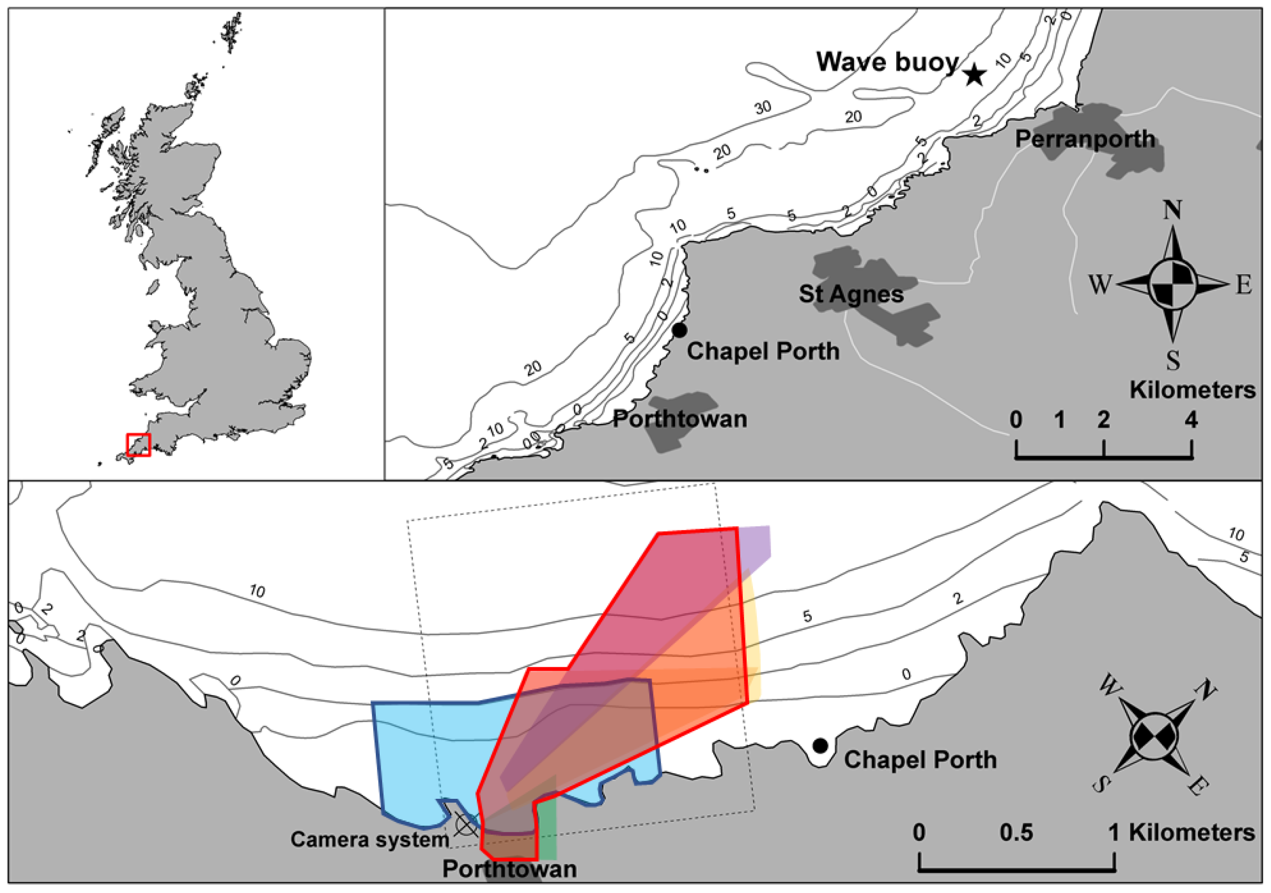
Figure 1.
Overview of the national and local orientation of field site in this study. The top left figure shows Great Britain. The red square indicates the focus area in the South–West of England. The top-right shows the regional situation. Local wave data is obtained from the wave buoy 5 km North–East of Porthtowan, close to Perranporth. The bottom figure represents the local situation. The blue area represents the typical area that could be covered by the Real-Time Kinematic GPS (RTK-GPS) topography surveys. The colored triangles indicate the footprint for each video-camera. The red-lined area shows the total video area. The shape of the total video area deviates from the traditional Argus [42] field of views (near 180 degrees alongshore view) due to the local geology, orientation and lenses of the cameras.

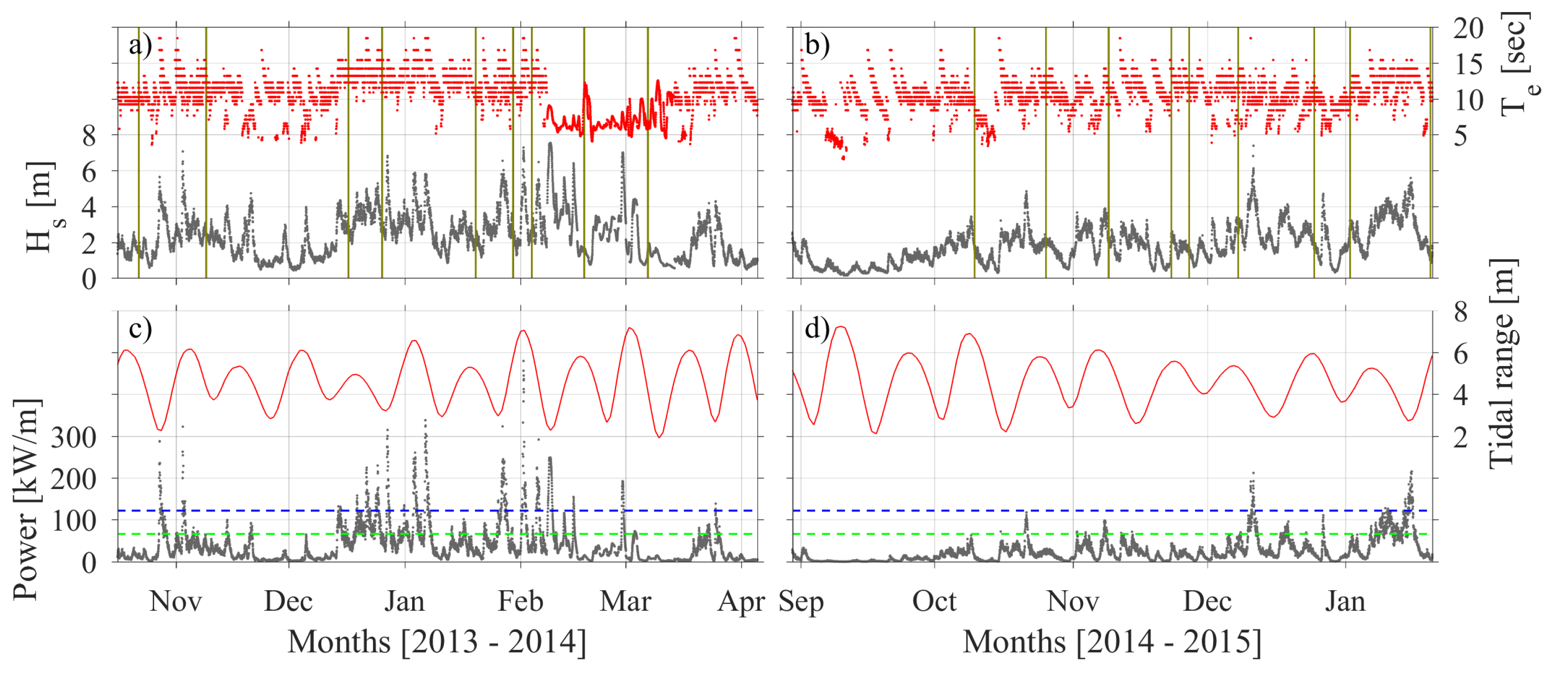
Figure 2.
Measured wave conditions for the 2013–2014 winter in the left column of figures and the 2014–2015 winter in the right column of figures. The significant wave height (metres) and energy period (seconds) are presented in (a,b). (c,d) show the total wave power in kiloWatt per wave crest length and tidal range in metres. The black lines correspond to the left-hand vertical axes and the red lines follow the right-hand vertical axes. In (a,b) the vertical green lines represent dates for the presented video-derived bathymetries. The horizontal dashed-lines in (c,d) represent the (blue) and (green) quantile exceedance threshold.

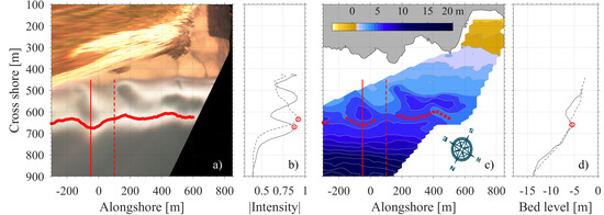
Figure 3.
Typical sub-tidal bar detection with Timex pixel intensities (a,b) and bathymetry estimate (c,d). Panel (a) shows an arbitrary projected Timex image with 1 × 1 m spacing and the vertical red line indicates an exemplary cross-shore transect on which the bar position is determined (similarly in c)). Panel (b) represents normalized pixel intensity over the red line shown in the projected Timex image. The bar detection using a video-derived bathymetry is shown in (c) with the corresponding profile in (d).

Figure 4.
Video-derived bathymetry sequence, (a–i), covering a period starting from 22 October 2013 (a) to 7 March 2014 (i). In between this period the projected images show arbitrary days depending on image quality and visibility of morphological features: (b) 9 November 2013, (c) 17 December 2013, (d) 26 December 2013, (e) 20 January 2014, (f) 30 January 2014, (g) 4 February 2014 and (h) 18 February 2014. The main morphological features are highlighted: sub-tidal bar is represented by the white dashed line, the green dashed lines indicate the positions of rip channels and the alongshore migration of morphological features (arrows).

Figure 5.
Morphology during calm conditions shown approximately every two months: 1 April 2014 (a), 4 June 2014 (b) and 14 August 2014 (c).
Figure 5.
Morphology during calm conditions shown approximately every two months: 1 April 2014 (a), 4 June 2014 (b) and 14 August 2014 (c).

Figure 6.
Video-derived bathymetry sequence covering a period from 10 October 2014 (a) to 20 January 2015 (i). Similarly to Figure 4 moments in between this period are shown in which (b) is 26 October 2014, (c) 9 November 2014, (d) 23 November 2014, (e) 27 November 2014, (f) 8 December 2014, (g) 25 December 2014 and (h) 2 January 2015.

Figure 7.
Longshore average bar position (dots) and standard deviation (bars) obtained from pixel intensities (red) and video-derived bathymetries (black) over time. Note that shore is at the bottom of the plots, offshore at the top.
Figure 7.
Longshore average bar position (dots) and standard deviation (bars) obtained from pixel intensities (red) and video-derived bathymetries (black) over time. Note that shore is at the bottom of the plots, offshore at the top.

Figure 8.
Alongshore averaged profiles partially computed using the inter-tidal beach surveys (a,c,e) and video-derived bathymetries (b,d,f). The dates used: (a,b) show 5 November 2013 (solid) and 30 April 2014 (dashed), (c,d) represent 30 April 2014 (solid) and 13 September 2014 (dashed) and plot (e,f) show 13 September 2014 (solid) to 5 December 2015 (dashed).

Figure 9.
The upper panel shows cumulative volume change on every survey-date since the start 6 November 2013 for the inter-tidal beach (blue), the sub-tidal area (grey and black) and the sum of both (red). The bottom plot presents hourly incident wave conditions over the same time-frame wherein the blue line indicates Hs, the black dots the energy period and the red dots correspond to the incident wave power per meter wave crest length. The error bars represent the daily standard deviation for the bathymetry estimates (black) and for the inter-tidal beach (blue) we presume that the RTK-GPS is reasonably 0.05 m accurate in the vertical.

Figure 10.
Traditional projected pixel intensity maps with overlaying video-derived bathymetry estimates (black-lines). Panel (a) represents the situation on 22 October 2013 and shows a transverse bar and rip beach state, (b) represents an “alongshore bar trough” beach state for the field of view on the 14 August 2014. Also in (b) there is a hint of bar welding around m indicating a TBR situation but in comparison to (a) with a larger alongshore wavelength. Panel (c) shows increased three-dimensionality. The bottom plots indicate the limitations of foam patterns. (d) highlights that during low-tide under low-energetic wave conditions the sub-tidal bar is invisible from pixel intensities. Alternatively, (e) represents a moment in time of high-tide and very energetic wave conditions resulting in a complete white surf zone and the sub-tidal bar is as well invisible.

Figure 11.
Sub-tidal bar detection using horizontally projected pixel intensities in (a,b) and bar detection using a video-derived bathymetry (c,d). Both applications are executed on data from the same day and same hour but with typically 20 min delay between the Timex and bathymetry (due to the collection set up). The vertical solid and dashed lines in (a,c) correspond to taken cross-sections as presented in respectively (b,d).

Table 1.
Inshore wave conditions during storms. Storm wave conditions are measured during the time that instant wave power exceeds the quantile threshold. represents the significant wave height (mean and maximum over the storm are respectively denoted as ¯ and . The corresponding average peak period and average wave direction over the total storm duration (Dur) are respectively indicated by and . TR means tidal range and indicates the water level at the peak of the storm intensity. ΣP is the accumulative hourly wave power over the duration of the storm.
| Date | [m] | [m] | [sec] | [°] | TR [m] | [m] | Dur [hrs] | ΣP [MW/m] |
|---|---|---|---|---|---|---|---|---|
| 27 October 2013 | 5.6 | 4.5 | 16.8 | 2.3 | 1.5 | 19.0 | 3.14 | |
| 2 November 2013 | 7.1 | 5.4 | 13.9 | 5.8 | 3.2 | 17.5 | 2.35 | |
| 14 December 2013 | 4.3 | 4.1 | 15.5 | 4.1 | 2.4 | 17.0 | 0.72 | |
| 19 December 2013 | 4.8 | 4.5 | 15.2 | 4.9 | 2.9 | 4.5 | 0.69 | |
| 21 December 2013 | 5.0 | 4.1 | 16.4 | 4.5 | 2.7 | 25.0 | 2.83 | |
| 24 December 2013 | 5.3 | 4.5 | 15.6 | 3.8 | 2.4 | 20.5 | 3.07 | |
| 27 December 2013 | 6.8 | 5.2 | 15.7 | 3.2 | 2.0 | 16.5 | 3.12 | |
| 3 January 2014 | 5.9 | 4.9 | 16.6 | 6.6 | 3.7 | 26.0 | 4.66 | |
| 6 January 2014 | 5.8 | 4.9 | 18.6 | 5.4 | 3.1 | 27.5 | 5.70 | |
| 25 January 2014 | 6.5 | 4.5 | 14.6 | 3.3 | 2.0 | 58.0 | 6.42 | |
| 1 February 2014 | 7.3 | 5.2 | 17.1 | 7.0 | 4.0 | 27.5 | 5.20 | |
| 5 February 2014 * | 6.5 | 4.9 | 15.9 | 5.2 | 2.9 | 20.0 | 3.25 | |
| 10 December 2014 | 7.4 | 5.0 | 13.7 | 4.5 | 2.7 | 19.5 | 2.87 | |
| 14 January 2015 | 5.6 | 4.6 | 14.2 | 2.9 | 1.9 | 43.5 | 4.54 |
* During this storm the wave buoy broke loose and stranded a few days later.
© 2019 by the authors. Licensee MDPI, Basel, Switzerland. This article is an open access article distributed under the terms and conditions of the Creative Commons Attribution (CC BY) license (http://creativecommons.org/licenses/by/4.0/).
Share and Cite
MDPI and ACS Style
Bergsma, E.W.J.; Conley, D.C.; Davidson, M.A.; O'Hare, T.J.; Almar, R. Storm Event to Seasonal Evolution of Nearshore Bathymetry Derived from Shore-Based Video Imagery. Remote Sens. 2019, 11, 519. https://doi.org/10.3390/rs11050519
AMA Style
Bergsma EWJ, Conley DC, Davidson MA, O'Hare TJ, Almar R. Storm Event to Seasonal Evolution of Nearshore Bathymetry Derived from Shore-Based Video Imagery. Remote Sensing. 2019; 11(5):519. https://doi.org/10.3390/rs11050519
Chicago/Turabian StyleBergsma, Erwin W. J., Daniel C. Conley, Mark A. Davidson, Tim J. O'Hare, and Rafael Almar. 2019. "Storm Event to Seasonal Evolution of Nearshore Bathymetry Derived from Shore-Based Video Imagery" Remote Sensing 11, no. 5: 519. https://doi.org/10.3390/rs11050519
Note that from the first issue of 2016, this journal uses article numbers instead of page numbers. See further details here.