Weakly Supervised Segmentation of SAR Imagery Using Superpixel and Hierarchically Adversarial CRF


1
School of Electronic and Information Engineering, Beihang University, Beijing 100191, China
2
Department of Informatics, University of Leicester, Leicester LE1 7RH, UK
3
Cognitive Big Data and Cyber-Informatics (CogBID) Laboratory, School of Computing, Edinburgh Napier University, Edinburgh EH10 5DT, Scotland, UK
*
Author to whom correspondence should be addressed.
Remote Sens. 2019, 11(5), 512; https://doi.org/10.3390/rs11050512
Submission received: 24 January 2019
/
Revised: 21 February 2019
/
Accepted: 26 February 2019
/
Published: 2 March 2019
(This article belongs to the Special Issue Superpixel based Analysis and Classification of Remote Sensing Images)
Abstract
:Synthetic aperture radar (SAR) image segmentation aims at generating homogeneous regions from a pixel-based image and is the basis of image interpretation. However, most of the existing segmentation methods usually neglect the appearance and spatial consistency during feature extraction and also require a large number of training data. In addition, pixel-based processing cannot meet the real time requirement. We hereby present a weakly supervised algorithm to perform the task of segmentation for high-resolution SAR images. For effective segmentation, the input image is first over-segmented into a set of primitive superpixels. This algorithm combines hierarchical conditional generative adversarial nets (CGAN) and conditional random fields (CRF). The CGAN-based networks can leverage abundant unlabeled data learning parameters, reducing their reliance on the labeled samples. In order to preserve neighborhood consistency in the feature extraction stage, the hierarchical CGAN is composed of two sub-networks, which are employed to extract the information of the central superpixels and the corresponding background superpixels, respectively. Afterwards, CRF is utilized to perform label optimization using the concatenated features. Quantified experiments on an airborne SAR image dataset prove that the proposed method can effectively learn feature representations and achieve competitive accuracy to the state-of-the-art segmentation approaches. More specifically, our algorithm has a higher Cohen’s kappa coefficient and overall accuracy. Its computation time is less than the current mainstream pixel-level semantic segmentation networks.
1. Introduction
The latest technology of synthetic aperture radar (SAR) imaging sensors can achieve all-day and high-resolution imaging for various geographical terrains [1,2]. SAR image segmentation aims at assigning optimal labels to the pixels and is considered as a foundation for many high-level interpretation tasks. Accurate segmentation can greatly reduce the difficulty of subsequent advanced tasks (target detection, recognition [3], tracking, change detection [4], etc.). Unlike the common classification framework, where classifiers (e.g., support vector machine (SVM) [5], random forest (RF) [6], sparse representation [7]) are generally used to assign a discrete or continuous label to each unit, segmentation models also need to preserve neighborhood consistency. For instance, in the segmentation framework, if the neighbors of a pixel are oceans, the confidence that it belongs to ocean areas should increase. The current mainstream segmentation algorithms include: superpixel segmentation methods [8,9], watershed segmentation methods [10,11], and level set segmentation methods [12,13].
As a representative probabilistic graphical model, conditional random fields (CRF) [14] can capture the appearance and spatial consistency and has become a fundamental tool in image segmentation. CRFs [14] deduces the conditional distribution of the labels given observations. In typical CRF-based segmentation methods [15], appropriate features are first extracted and selected from the input images, then structured support vector machine (SSVM) [16] or other classifiers are utilized to learn the coefficients of CRF for segmentation [17,18]. Hence, the quality of the feature descriptors has a significant impact on the performance of CRF-based segmentation models. In order to further accelerate the segmentation speed for large-scale SAR images, the input generally is over-segmented into superpixels [19,20]. However, effective feature extraction algorithms for superpixels remain a challenge. Most of the previous methods focus on hand-crafted features for superpixels, e.g., histogram of oriented gradients (HOG) [21], gray-level co-occurrence matrix (GLCM) [22], and co-occurrence matrix (COOC) [23]. These hand-crafted features include many coefficients determined by previous knowledge and experiences in practice [19], which is difficult and time-consuming. Besides, the speckle noise existing in SAR images also increases the difficulty of feature extraction.
In recent years, deep convolutional neural network (DCNN) [24] has achieved tremendous breakthroughs in the field of image classification and segmentation [25,26]. Combining CRF and DCNN for SAR image segmentation has become a research hotspot [27,28]. For example, Liu et al. [15] utilized the CNN trained on the ImageNet dataset to extract features of superpixels. Liu et al. further modeled the feature extractor and continuously valued CRF as a DCNN in [27], achieving better results compared with hand-crafted features on the depth estimation and semantic segmentation tasks.
However, the CNN based feature descriptor still has s several issues that need to be resolved. First, either DCNN or hand-crafted extractor neglects the neighborhood label consistency. According to a human’s a priori knowledge in labeling a superpixel, the context information from its adjacent superpixels have a strong influence towards the superpixels labeling. For example, a superpixel surrounded by farmland areas is highly likely to be farmland.
In addition, training DCNN needs a large number of labeled samples, which mainly come from manual annotation and are quite labor-intensive, especially when using SAR images. Unlike the common optical images, there is not any universal and large scale labeled SAR image dataset like ImageNet, which can be applied to interpreting SAR images. Each airborne SAR imaging system has distinctive imaging parameters. Even for the same airborne SAR, due to the change of altitude, speed, and overlook angles in each flight, the features of the same target regions are always different. Hence, for various SAR data datasets, we need to manually label the training sets. Hence, researchers have proposed unsupervised learning models, such as sparse auto-encoder (SAE) [29], restricted Boltzmann machine (RBM) [30], deep belief network (DBN) [31], and generative adversarial nets (GAN) [32]. Among them, GAN is a new unsupervised learning model proposed in 2014 and has been successfully applied in image generation, image inpainting, road segmentation [33], etc. This model is composed of a generator (G) and a discriminator (D). The G network attempts to generate fake images to deceive the discriminator, while the discriminator is a binary classifier and endeavors to distinguish the fake data from the real one. The adversarial training process between the two sub-networks enforces the discriminator to achieve a better feature extraction ability than the other unsupervised deep learning models.
In this paper, we propose a superpixel-wise hierarchically adversarial CRF (HACRF) which combines GAN with CRF to address the above problems. First, in order to reduce the computational cost while maintaining the edge information of the input image, the input is over-segmented to superpixels. Second, based on the semi-supervised conditional generative adversarial nets (CGAN) [34], we design a hierarchical CGAN to learn the target superpixels and their background through the adversarial training process. Then the concatenated feature vectors are fed into the CRF model to obtain the optimal segmentation results. The novel aspects of our proposed algorithm consist of the following aspects.
(1) To improve the SAR image segmentation performance with insufficient labeled samples, we introduce the CGAN in CRF-based segmentation method. In the CGAN, a multi-classifier is added in the original GAN, which shares the feature extraction network with the discriminator. The binary discriminator aims at distinguishing between the real samples and the generated samples, and the multi-classifier strives to label the samples correctly. Hence, the feature extraction layers can simultaneously learn the parameters using insufficient labeled images and abundant unlabeled images.
(2) In order to preserve neighborhood label consistency during the feature extraction, the hierarchical CGAN model is composed of two CGANs, named target CGAN (TCGAN) and background CGAN (BCGAN). For an input superpixel (named target superpixel), we also extract a background superpixel of a larger size, which is composed of the neighboring superpixels of the target superpixel. TCGAN aims at learning the feature vectors from the target superpixels, while BCGAN is introduced to explore the corresponding background superpixel’s features. The concatenated feature vectors from two kinds of features are then fed into the CRF, approximating maximum a posteriori (MAP) of the labels.
The rest of this paper is organized as follows. Previous CRF-based segmentation approaches are reviewed in Section 2. Section 3 presents the proposed method, including the generation of the target and background superpixels, training hierarchical CGANs, and superpixel-wise segmentation using conditional random field. Our experiments and the results are presented in Section 4. Section 5 presents the discussion in terms of pros and cons. Section 6 gives the conclusion.
2. Related Work
In this section, we review the previous CRF-based approaches for image segmentation, which are closely related to our method. Their merits and defects are distinctly summarized in Table 1. The earlier way of applying CRF for segmentation is directly processing each pixel as a unit [16]. These methods do not need the feature extraction step, while their weakness is the heavy computing burden. Taking a fully connected CRF [35] as an example, for an image with pixels, edges are required to calculated when build the graph model. Considering remote sensing images generally have much larger sizes than optical images, the pixel-wise segmentation methods’ calculation will sharply increase.
With appearance of superpixel generation models (e.g., simple linear iterative clustering, SLIC [36]), the superpixel-wise segmentation algorithms have received considerable attention, which introduce CRFs as a post-processing to incorporates the structured constraints. Most of the superpixel generation models employ the unsupervised clustering algorithms to cluster the adjacent and similar pixels together to form a superpixel. Superpixels can greatly improve the efficiency of the segmentation algorithm while preserving the images’ edge information. According to the different kinds of superpixel feature descriptors, these superpixel-wise segmentation methods can be divided into two parts, one of which uses the traditional hand-crafted methods to extract superpixel features. For instance, Sultani W et al. [19] introduces a feature descriptor for superpixel, including HOG, GLCM, intensity histogram (IH), and mean intensity (MI). The weight of each type of the features are learned also by SSVM. Kenduiywo B K et al. [37] selects gray-level GLCMs based on a 3 × 3 convolution matrix with 64 gray-scale quantization levels as the features to train the CRF. Moreover, some filter sets, such as Gabor and wavelet transform, are also utilized for extracting complex features [38]. Most of these methods are unsupervised and do not require labeled samples. However, their parameters are often based on empirical evidence.
Later on, more attempts are made towards extracting deep feature descriptors for superpixels. These methods first train a DCNN to extract the features, then apply a CRF model to refine the segmentation results [15,27,39]. In these models, feature extraction and CRF inference are still separated. Recently, a more appealing direction is to facilitate deep end-to-end segmentation. For example, Zheng S et al. [40] treats mean field inference in CRFs as a recurrent neural network (RNN). Lin et al. [41] present to learn the unary and pairwise potentials of CRFs using CNNs. The above-mentioned deep feature descriptors all need a large number of labeled images for training the DCNN. In contrast, here we explore GAN to make the best use of the abundant unlabeled SAR images in CRF inference.
3. Hierarchically Adversarial CRF
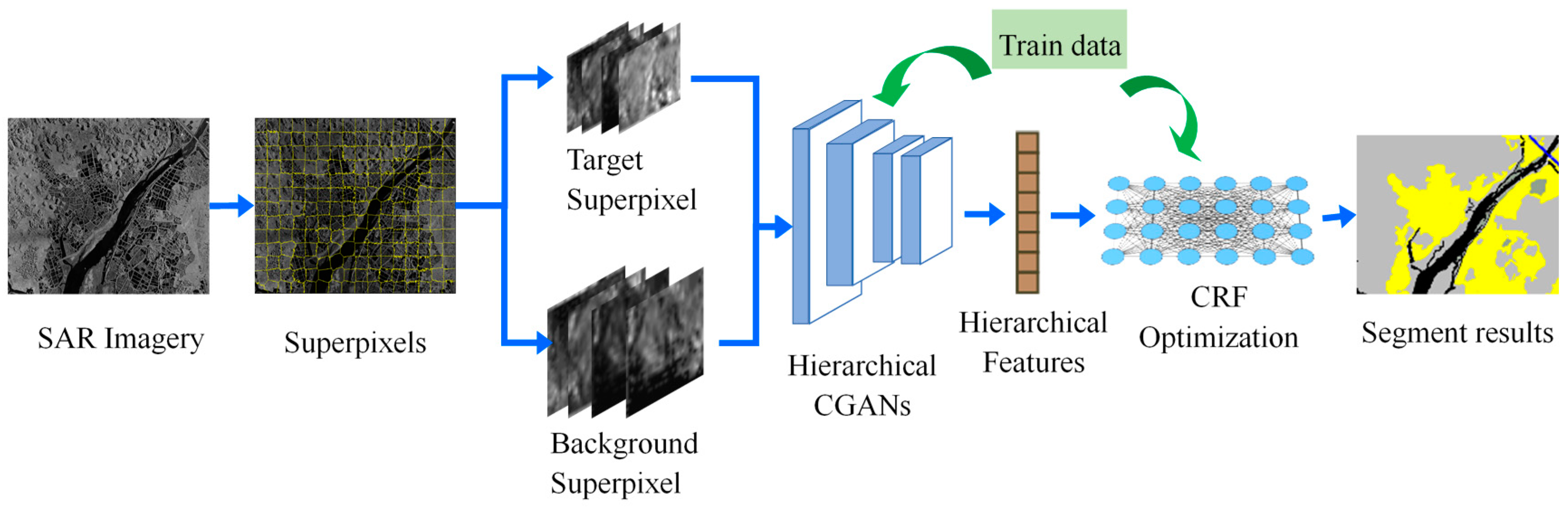
This paper presents a hierarchical adversarial CRF (HACRF) method to segment the large-scale SAR images. As shown in Figure 1, the segmentation processing can be divided into three steps: (1) over-segment the input SAR images to target superpixels and background superpixels; (2) two kinds of superpixels are fed into the hierarchical CGAN to extract their feature vectors, which are composed of target CGAN (TCGAN) and background CGAN (BCGAN); (3) the concatenated features are then utilized to train the CRF and infer the optimum label of each superpixel. The training of hierarchical CGAN is performed using the labeled data and unlabeled data from the testing set. The unary and pairwise potential coefficients of CRF are learned by SSVM.
3.1. Target Superpixels and Background Superpixels
Whether it is in training or testing, we need to first over-segment the large-scale airborne SAR images into superpixels using the SLIC proposed in [36]. Compared with the regular rectangular patches used in deep learning, superpixels can preserve the edge information of the scene, while effectively speeding up the segmentation algorithm to meet the real time requirements in remote sensing. We represent the superpixels obtained from all the training images in the dataset as , where is the number of the superpixels.
In order to process the irregular superpixels by convolution operation, we place each superpixel into a rectangular patch. The central of the patch corresponds to the centroid of the superpixel. This kind of patch is called ‘target superpixel’, denoted as .
When manually labeling a superpixel, we find that it is difficult to determine its category if only focusing on the target superpixel without noticing the surrounding superpixels. For example, the shadow areas of mountains look very similar to river areas in airborne or spaceborne SAR images. Therefore, in order to distinguish a superpixel’s class, taking its background information into consideration is necessary. If there is a clear difference between the central superpixel and the surrounding superpixels, the target superpixel is likely to be located in the shadow of the mountains, otherwise, it is in the river areas. Based on the above considerations, we believe that appearance and spatial consistency should also be taken into account in the feature extraction stage, in other words, both the background and target information should be considered. Therefore, for a superpixel , a larger rectangular region centered on the centroid of the superpixel is selected as the background slices, called the ‘background superpixel ()’. It should be noted that we set the label of to be the same as that of . It forces the hierarchical CGAN to extract the background information with the label of the central superpixel.
3.2. Hierachical CGANs
In this section, a hierarchical CGANs is proposed to extract the features of the target and the background superpixels, aiming at mining useful information from the abundant unlabeled data and improving the performance of feature extraction. We will introduce the architecture of hierarchical CGANs in this section.
The original GAN is mainly composed of a generator and a discriminator. The generator converts the random noises following the distribution into the fake images by deconvolution. The fake images and the real images are fed into the discriminator, whose goal is to correctly discriminate whether the input image is real or fake. The generator attempts to keep the generated fake images as close to the real as possible until the discriminator cannot distinguish them. The adversarial training with the generator makes the discriminator achieves better feature extraction ability. However, the original GANs structure is unable to learn the label information. The conditional GANs (CGAN) [42] is then proposed to handle this drawback by adding a multi-classifier in the GANs network. This classifier shares the feature extraction network with the discriminator. Thus, the loss function of the CGAN is defined as
where stands for all the real images, including the labeled images and the unlabeled images; denotes the output of the discriminator. is the sum of for all the input , while denotes the sum of ,which represents the loss values of the multi-classifier for all the labeled data .
On the right-hand side of Equation (1), the first term ensures that the discriminator can correctly distinguish all the real and fake images; the second term encourages the fake images to deceive the discriminator; and the third term is to support the multi-classifier to correctly classify the labeled data.
More specifically, in each training epoch, we first fix the parameters of the generator and train the discriminator and the multi-classifier. The generated fake images and the real images are fed into the discriminator. The discriminator is optimized by maximizing the following loss functions with a stochastic gradient descent (SGD) algorithm
where refers to the number of all the real images . Meanwhile, the multi-classifier takes the labeled real images as the input to predict their labels and calculate the following loss function , whilst its parameters are then updated by minimizing the loss function
Here, refers to the number of labeled images .
During training of generator, we first fix the parameters of the discriminator and the multi-classifier. The faked images are fed into the discriminator, and then the generator’s parameters are optimized by minimizing the following loss function
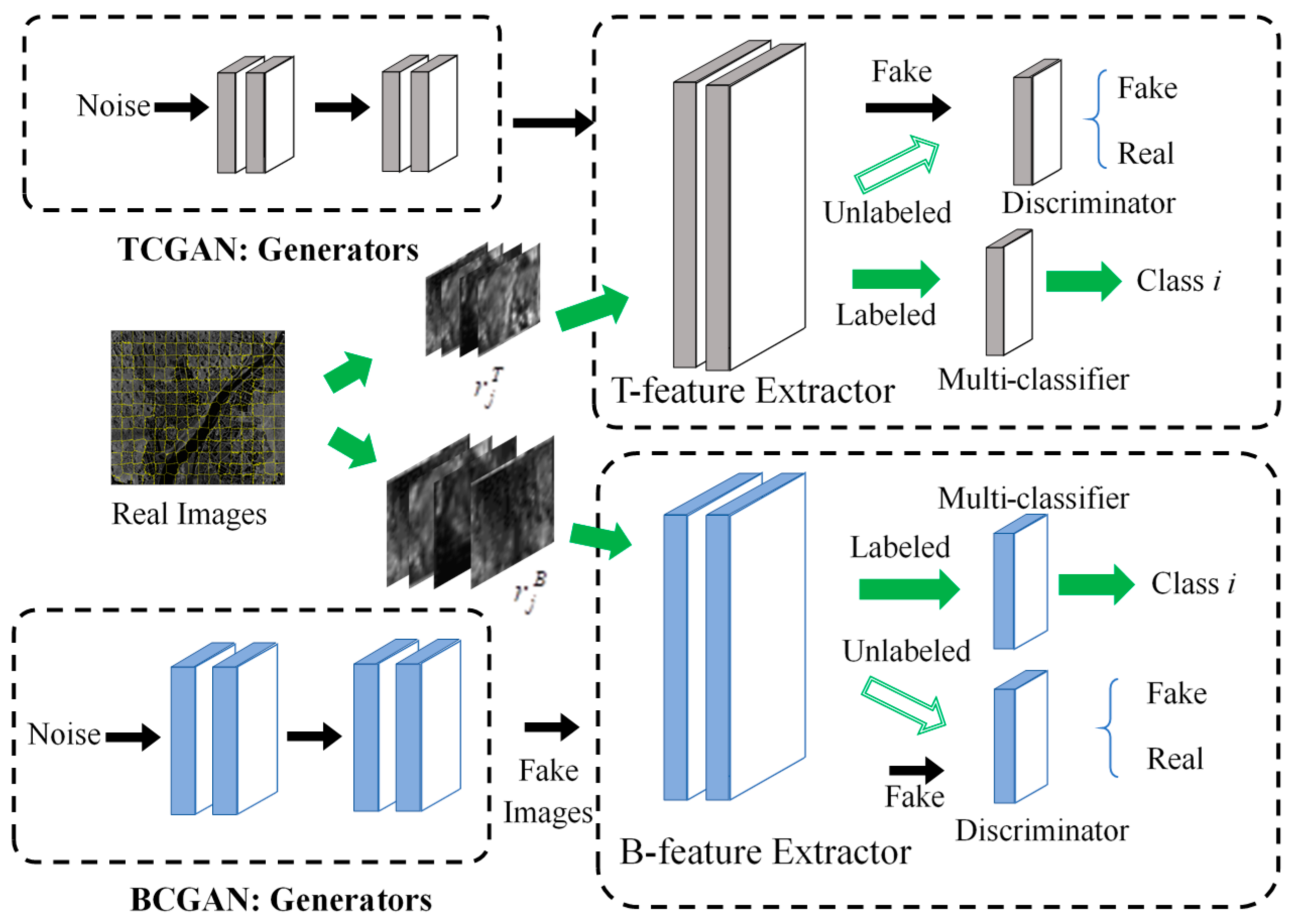
The proposed hierarchical CGANs includes dual CGANs: Target CGAN (TCGAN) and background CGAN (BCGAN). Figure 2 shows the structure and the training process of the hierarchical CGANs. TCGAN and BCGAN are trained independently. Taking the TCGAN as an example, the target superpixels from the training images include the labeled and the unlabeled, represented as and respectively. is the fake superpixel generated by the G-network of the TCGAN. In each training epoch, , , and are fed as the input of the feature extraction part of the TCGAN (named T-feature extractor). Then the discriminator aims at distinguishing whether the three kinds of feature vectors are real or fake and obtains the loss value in Equation (5). Meanwhile, we use the multi-classifier to predict the categories of the labeled target superpixels and calculate the corresponding loss value in Equation (5).
where , , and denote the numbers of the labeled, unlabeled and generated target superpixels. The parameters of the T-feature extractor, discriminator, and multi-classifier are updated by maximizing the .
The fake target superpixels are then employed to train the G-network of the TCGAN by minimizing the following loss function
The adversarial learning between the discriminator, multi-classifier, and generator can fully exploit the available information in the unlabeled target superpixels, and thus improve the performance of the T-feature extractor. The training process of the BCGAN is similar to the TCGAN. The labeled background superpixels , the unlabeled background superpixels and the generated superpixels are together fed into the B-feature extractor of the BCGAN, and then the loss values can be calculated based on the outputs of the discriminator and multi-classifier. The parameters of the B-feature extractor, discriminator, and multi-classifier are optimized by maximizing . In the testing stage, the trained dual feature extractors are employed to extract the features of the target superpixels and the background superpixels respectively, which are denoted as and respectively.
3.3. Superpixel-Wise Segmentation Using Conditional Random Field
The final feature vector of a superpixel is obtained by concatenating the features and . In this section, conditional random fields (CRF) is introduced to optimize the superpixel-wise segmentation results according to the input features. CRF is first proposed by Lafferty et al. [14] as a data labeling method based on a graph model. For an input SAR image with superpixels , the labels assigned to these superpixels are defined as , where and refers to the number of the classes. CRF models the whole image as an undirected graph model , where is the set of vertices and each superpixel corresponds to a vertex. represents the set of edges. It has been demonstrated that in CRF, the conditional probability distribution of label obeys the following Gibbs distribution,
where stands for the set of cliques in the graph model; are the coefficients of CRF model, and is a normalized constant term. denotes the potential function of the cliques given the observation and the corresponding labels . For regular image classification and segmentation, unary and pairwise potentials will be included in the objective function. In this case, Equation (7) can be rewritten as
where denotes the label value of and stands for all the surroundings superpixels of the central superpixel . On the right-hand side of Equation (8), is the unary potential, indicating the dependence between and its label , and is the coefficient set of unary potential. Similarly, denotes the pairwise potential, where is its coefficients and represents all the adjacent superpixels of superpixel . Pairwise potential aims at assigning the similar labels to the superpixels with consistent features. At this point, the CRF optimization can be expressed as
It indicates that the label sequence achieving maximum a posteriori (MAP) will be the optimal label . Since is a constant relative to , the formula can be simplified as
In this formula, the observation refer to the superpixel features of the input SAR image, i.e., . Hence, we can have . We design the unary potential as a linear combination of the features and coefficients, i.e.,
where refers to the probability that the superpixel is assigned to the label yi given feature vector ; coefficient is a matrix with the size of , represents the number of the classes, indicating the length of the feature vector .
Next, we define the pairwise potential as
where [.] indicates zero-one indicator function. is an element of the transition matrix with the size of , representing the possibility that a superpixel adjacent to a superpixel belonging to is labeled as . As the graph is undirected, is a symmetric matrix. represents the distance between the feature vectors of two superpixels and , which is defined as
where is the element of feature vector . is proportional to the difference between the superpixels’ features. Equation (13) encourages CRF to assign different labels to neighboring and distinctive superpixels.
In summary, CRF coefficients include , and we introduce the SSVM to train the model with the coefficients. Finally, an inference algorithm is used to calculate the MAP , and find the optimal label sequence . Here we use the AD3 proposed in [43] to estimate the MAP inference. AD3 is a dual decomposition algorithm based on the alternating directions method of multipliers. As each local subproblem has a quadratic regularizer, AD3 converges faster than other subgradient-based dual decomposition and message-passing methods. Experimental results also prove that AD3 can result in good segmentation.
The pseudo code of the proposed method is presented in Algorithm 1, which explains the training of the hierarchical CGANs and CRF in details.
| Algorithm 1: Hierarchical Adversarial CRF (HACRF) based Image Segmentation |
| Input: Training images , test images Output: Superpixel-wise segmentation of image procedure Training Hierarchical CGANs.  procedure Training CRF
|
4. Results
4.1. Data Description
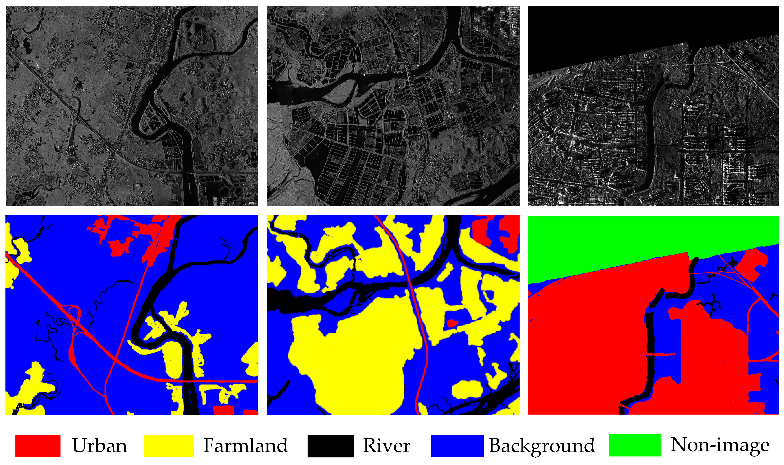
The SAR database used in our experiment contains the imaging results of FangChengGang in Guangxi Province, China [44]. The imaging range of this database is about 30 × 30 km with a resolution of 2 m, and image size is 1122 × 1419 pixels. There are totally 36 images in the dataset and seven of them are selected as the training set. We manually annotate these images into five classes: farmland, river, urban, background, and non-image. Non-image refers to those unscanned areas during the imaging, whose pixel values are zero. Three exemplar images and the corresponding ground truth maps are illustrated in Figure 3. In the ground truth, different colors represent various categories. As can be seen, there are various topographic and geomorphic conditions—e.g., complex buildings and roads, and dense river networks characterized by different sizes and shapes—leading to great difficulty in segmentation.
In the training or testing stage, all the images and the corresponding ground truths are first over-segmented to the superpixels using the SLIC method. The size of the superpixel determines the resolution of the segmentation results. The larger superpixels are, the more edge information in each superpixel will be missed. For example, some rivers with a width smaller than that of the superpixels will be lost. A small size of superpixels also will increase the computation of the segmentation algorithm. According to the clustering results of the SLIC for the FangChengGang dataset, a superpixel with 200–300 pixels can ensure that each superpixel retains the shape of rivers and urban areas. In the experiment, we set the compactness of the SLIC to be 0.5 and the number of the superpixels for each SAR image (1122 × 1419 pixels) is 8000, which means a superpixel contains an average of 200 pixels. The size of the patch named ‘target superpixel’ is set to be 16 × 16, so that each patch can accommodate an irregular superpixel. The background superpixels’ sizes are set to be 16 times the target superpixel, i.e., 64 × 64.
Table 2 gives the numbers of all the classes of the superpixels in the training and testing sets, and the percentages of the training pixels in the overall pixels with respect to each class. It can be seen that the numbers of urban, farmland, and river superpixels are basically the same both in the training and testing sets, while the number of the background superpixels is much larger than that of the other three categories. This is consistent with the practical application. In practice, there are many kinds of land species in the large scene, but we are only interested in a small part of them. The huge imbalance in the numbers of the samples presents a challenge for the segmentation models. The experiments are implemented using Pytorch in an Ubuntu platform. The main configuration of our computer is 32 G Memory, Intel(R) Xeon(R) CPU L5639 @ 2.13GHz×12 (Intel, Santa Clara, CA, USA) and Tesla K20c graphics (NVIDIA, Santa Clara, CA, USA).
4.2. Evaluation Measures
The pixel-wise overall accuracy (OA) [45], overall precision (OP) [46], and F1 score [47] are utilized to quantitatively measure the segmentation results of each method. F1 score is the weighted harmonic of precision and recall as
The precision refers to the proportion of the pixels correctly assigned in all the segmentation results, while the recall value corresponds to the ratio of the pixels segmented correctly in all the pixels in the ground truth. The larger the F1 score, the better the overall performance of the segmentation algorithm. OA and OP are defined as the weighted average recall values and precision values, respectively. Cohen’s kappa coefficient (κ) [48] is also introduced to measure the correctness of the segmentation. The definition of the Kappa coefficient is
where is named as the relative agreement between the segmentation results for the testing data and the real labels; is the hypothetical probability of the chance agreement. A coefficient closer to 1 denotes the better agreement between the segmentation results and the ground truth.
4.3. Feature Extraction Analysis
In this section, before measuring the segmentation results, we first visualize the features extracted by the hierarchical CGANs to explore whether our feature extraction method can capture the inherent differences between various kinds of superpixels. We train the hierarchical CGANs using the labeled superpixels from the training set and the abundant unlabeled superpixels from the testing set to obtain the T-feature extractor and B-feature extractor.
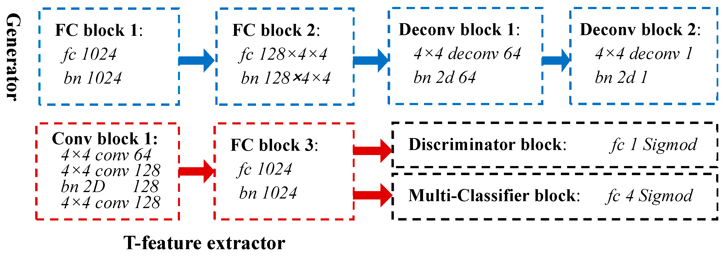
Figure 4 shows the architecture and hyperparameters of the TCGAN. The abbreviation ‘bn’ and ‘FC’ correspond to the batch norm and fully-connected layers. The generator (blue rectangles) is composed of two fully-connected blocks (FC block 1 and 2) and two deconvolution blocks (Deconv block 1 and 2). The T-feature extractor (red rectangles) consists of the convolution block 1 and the FC block 3, which is responsible for transforming a 16 × 16 target superpixel into a feature vector of 1 × 1024.
The default activation functions for all the layers are Leaky ReLU [49]. The cross entropy and binary cross entropy are selected as the loss functions of the multi-classifier and the discriminator. The experimental results show that when the training epoch of the TCGAN is greater than 30, the segmentation performance will not continue to improve, so we set the epoch number as 30. Moreover, the variation of the batch size and learning rates of the discriminator, the multi-classifier, and the generator have little effect on the performance of the segmentation in our experiment, and therefore we set the batch size to 1 and set all learning rates to 0.0002.
The architecture of the BCGAN remains the same, except the neuron number of its FC block 2 is set to be 128 × 16 × 16. Similarly, the B-feature extractor converts each background superpixel with size 64 × 64 into a 1 × 1024 feature vector. After that, the final feature vector of the superpixel (1 × 2048) is obtained by concatenating the above dual features vectors.
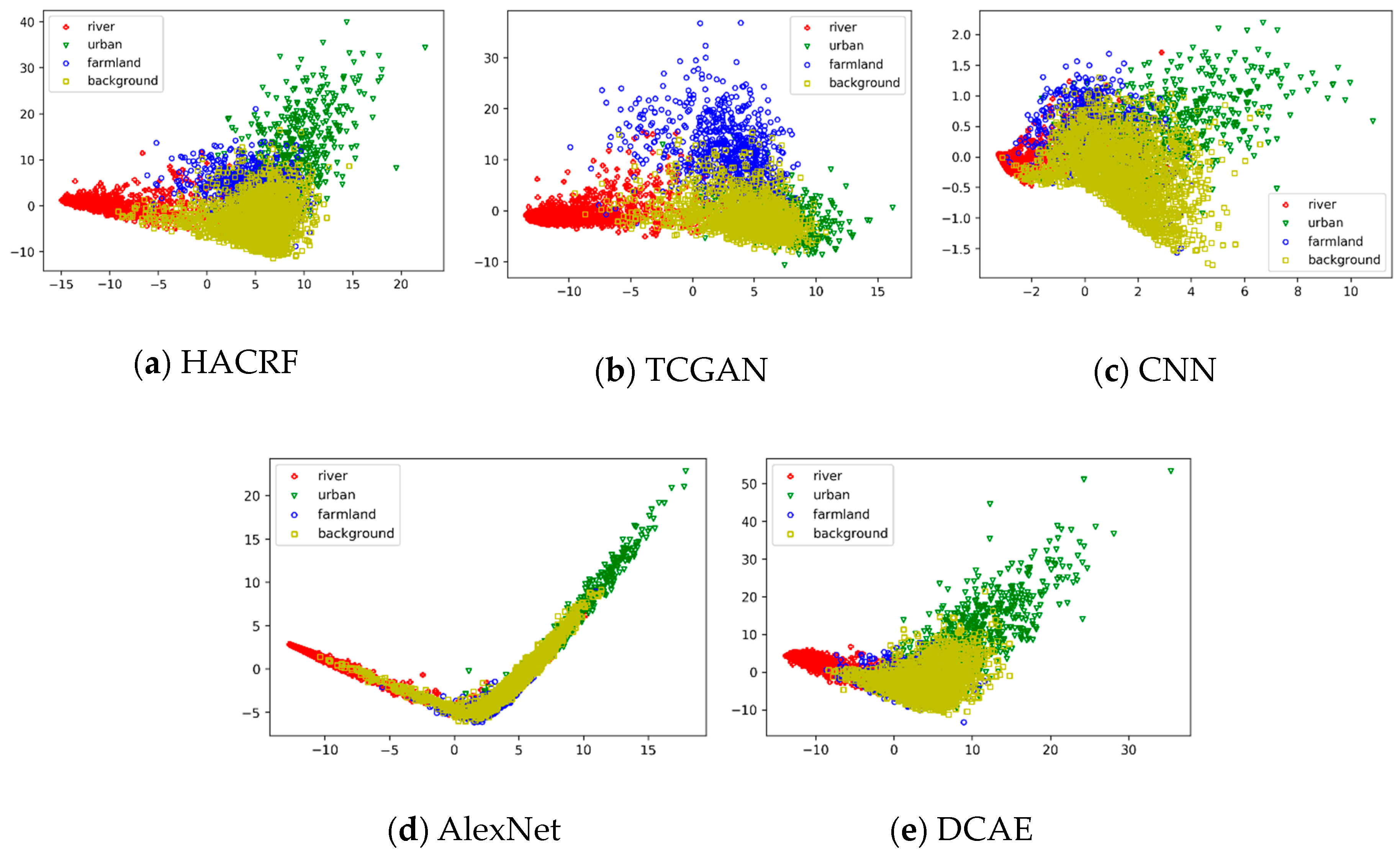
In order to easily visualize the distribution of features, we use principal component analysis (PCA) [50] to reduce the dimension of the feature vectors to two dimensions. The results are illustrated in Figure 5a, where individual colors and markers are utilized to distinguish the different kinds of features. It can be seen that different classes of features extracted by the HACRF do not show much confusion. For comparison, we also visualize the features extracted by other models, as shown in Figure 5b–e. Figure 5b shows the features only extracted by the T-feature extractor, where a large number of the feature points of the background and urban areas are overlapped, proving the introduction of background features can improve the separability of the features. Figure 5c illustrates the features extracted by a supervised CNN. This CNN is composed of the T-feature extractor and the multi-classifier from the TCGAN, so its hyperparameters are also consistent with the TCGAN network. This supervised CNN is trained using 16 × 16 target superpixels from the training set (epoch = 100). Severe confusion between different kinds of features happens in the CNN’s results, which will inevitably reduce its accuracy of the segmentation results.
Figure 5d shows the distribution of dimension-reduced features from the AlexNet, which is composed of the convolution and pooling layers of AlexNet [51] network pre-trained on ImageNet [52] as the feature extractor. The feature extractor outputs a 256-dimensional feature vector. Figure 5e also gives the distribution of features extracted by the DCAE model, which is an autoencoder-based classification method proposed in [38]. In particular, the extracted GLCM and Gabor features first go through dimension reduction by average pooling and PCA. Then the dual-layer sparse autoencoder is employed to optimize these features. Finally, the optimized features are classified using a fully-connected layer with the Softmax activation functions. The number of the units in the first hidden layer is set to 1.5 times larger than the input dimension, and the number of the second hidden layer’s units is set to 0.8 times smaller than the input dimension. The greedy training method is utilized to train the autoencoder. The hyperparameters of this algorithm are set as follows: the loss function is the mean square error function; the learning rate is 0.0001; the batch size is also 330; the training epoch number is 40. The 16 × 16 patches are cropped from the input SAR images with a step size of 16. In summary, for either AlexNet or DCAE, the separability of each class features is weaker than that of the first three methods.
4.4. Segmentation Comparison
After converting each superpixel into a feature vector, we can model a SAR image as an undirected graph, where superpixels are regarded as the vertices of the graph, and adjacent superpixels are connected by edges. Finally, SSVM is employed to update the coefficients of the graph-based CRF. The optimal segmentation results can be obtained by the AD3 algorithm.
In this part, we compare the segmentation performance of our HACRF method with several methods, such as TCGAN-CRF, CNN-CRF, AlexNet, DCAE, and SegNet [53]. Among them, the TCGAN-CRF only adopts the T-feature extractor in the TCGAN to extract the superpixels’ features. The other parts and parameters are consistent with those of the HACRF. The comparison with the TCGAN-CRF allows us to explore whether or not introducing background feature extraction can improve the segmentation results. In the CNN-CRF, a fully supervised CNN network mentioned in the feature extraction analysis section, instead of the hierarchical CGAN, is applied to extracting the features. The CNN is composed of the T-feature extractor and the multi-classifier in the TCGAN. In order to avoid the influence of the change of hyperparameters on the segmentation results, its hyperparameters also are consistent with those of the TCGAN.
AlexNet refers to the classification method based on the AlexNet proposed in [54]. This algorithm combines the AlexNet-based feature extractor (described in Section 3.3) and a fully connected network with Softmax functions for classification. During the training of the network, the parameters of the convolution and pooling layers in AlexNet are fixed, and the patches from the training set are used to train the full connected layers. According to the suggestion of [54], the input patches with measuring 21 × 21 are cropped from the training images with a step size of 10. The loss function is the mean square error function; the learning rate is set to 0.0001; the batch size is set to 330; the training epoch is 40; and the regularization parameter is set to 0.0005.
SegNet is an encoder-decoder network for performing pixel-level semantic segmentation proposed in [53]. The encoder part uses the first 13-layer convolutional network of VGG16 [55] pre-trained on the ImageNet. Each encoder layer corresponds to a decoder layer, and the decoder employs pooling indices calculated in the max-pooling operation of the corresponding encoder to execute upsampling. Then the upsampled maps are convolved with the trainable filters to produce dense feature maps. The feature maps are sent to the Softmax classifier to generate the class probability for each pixel. It has been found that in the SAR image dataset, a larger patch size more easily causes unstable convergence of the training, leading to poor segmentation results. Hence, we finally set the patch size to 16 × 16. Among the other hyperparameters, the learning rate is 0.01, the regular regularization parameter = 0.0005, batch size = 300, and training epoch = 50.
Table 3 compares the segmentation results of several methods for FangChengGang testing set. Obviously, our method is superior to other methods in OA, OP, F1 scores, and Kappa coefficient. Notably, the better metrics of HACRF than TCGAN-CRF show that the introduction of background information in the feature extraction step not only enhances the separability between different classes of superpixel features, but also improves the segmentation results. In addition, TCGAN-CRF performs much better than CNN-CRF, proving that weakly supervised CGAN network does have better feature extraction ability than supervised CNN network. AlexNet has the lowest OA, OP, F1 scores and Kappa coefficient. On the one hand, as a fully supervised method, AlexNet requires a large number of labeled samples. On the other hand, AlexNet and DCAE are both classification algorithms, and they do not preserve neighborhood label consistency. All four evaluation indicators also show that among the six algorithms, SegNet’s segmentation performance is only slightly worse than HACRF and better than the other four methods. It benefits from its encoder–decoder structure which can implement the appearance and spatial consistency using convolution and deconvolution layers. The excellent feature extraction capability of the deep network improves its segmentation performance.
Table 4 gives the F1 scores of multiple methods for each class of superpixels. In detail, HACRF’s F1 scores for urban areas and farmland are highest in all methods, respectively 63.17 and 70.63. SegNet’s scores for these two classes are only 61.46 and 52.56. Farmland is the hardest class to segment. AlexNet and DCAE’s F1 scores are both less than 30, and SegNet’s is only 52.56. Conversely, TCGAN-CRF’s F1 score for farmland regions is 63.08, which is more than the CNN-CRF’s (50.42), indicating that the introduction of TCAGN effectively improves the segmentation results. The addition of BCGAN further increases the F1 score of HACRF to 70.63. For river areas, the F1 scores of all methods are approximately equal and all greater than 72, demonstrating that river features are simpler and easier to segment than farmland and urban areas. To be more specific, SegNet achieves the best score on the class of river (75)—a little higher than HACRF (73.67) and TCGAN-CRF (72.76)—for the background areas, although SegNet gets the highest score, which is only about 2.33 more than the proposed HACRF. From the above analysis, SegNet is lower than HACRF in terms of OA, OP, F1 scores and Kappa coefficient, mainly because its unacceptable segmentation effect on the complex farmland regions.
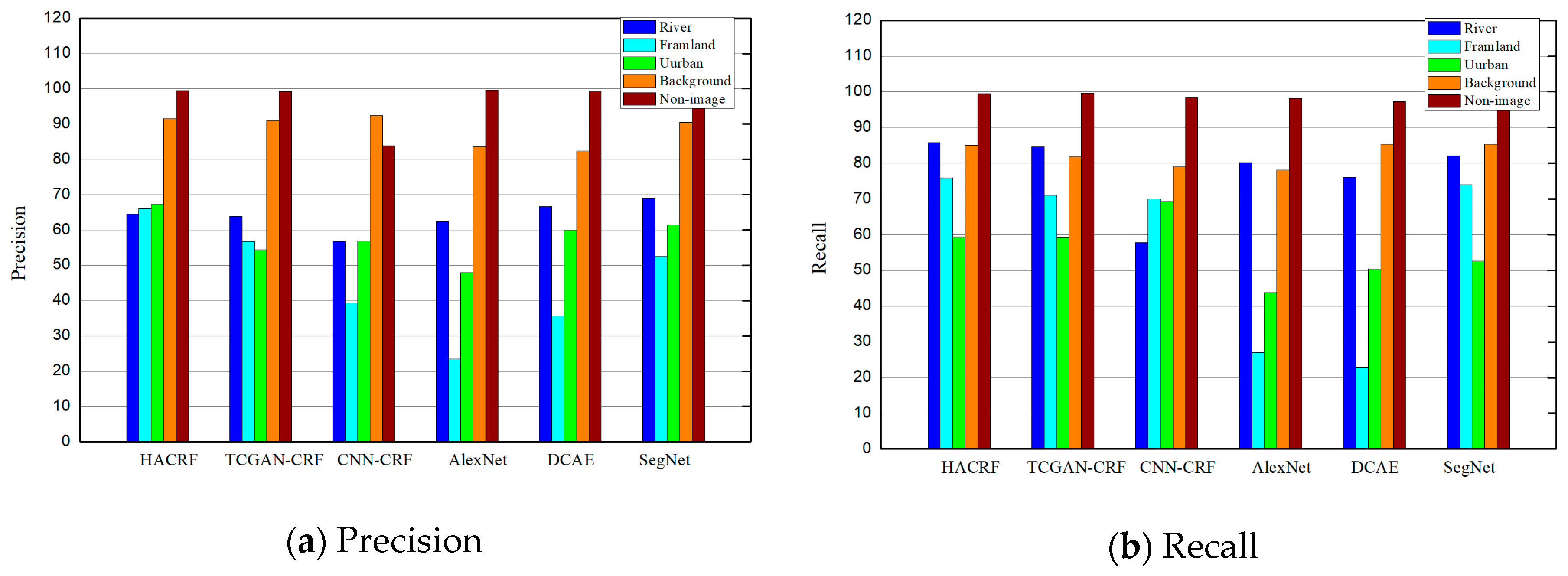
In addition, Figure 6 compares the pixel-level precision and recall values of the six methods, respectively. In Figure 6a, HACRF has greater precision of 65% for river, farmland and urban pixels. In the segmentation results of TCGAN-CRF, AlexNet, and DCAE, only their precision for river areas is higher than 60%. SegNet just has segmentation precision of more than 60% for farmland and urban areas. Figure 6b shows that recall values of our method for five classes of pixels are all higher than 60%. Conversely, TCGAN-CRF, AlexNet, DCAE, and SegNet’s recall values for urban pixels are all lower than 60%.
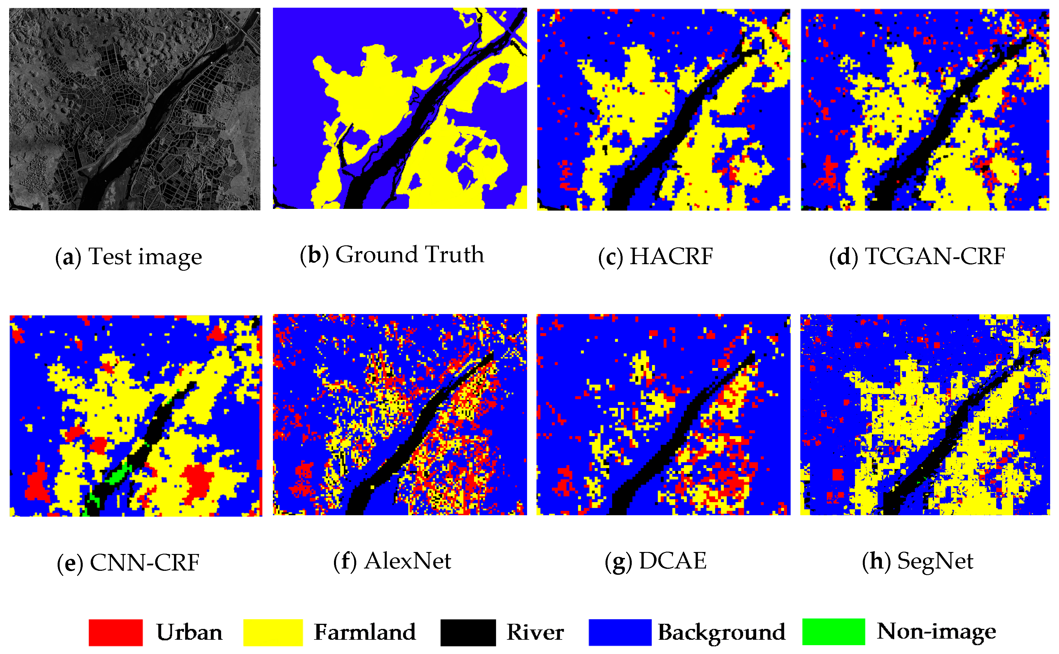
In order to visually compare the segmentation results of each method, we draw the segmentation results of several methods for two testing images in Figure 7 and Figure 8. The input image in Figure 7 is mainly composed of river and farmland areas, which are both segmented accurately by the HACRF. Although the TCGAN-CRF and CNN-CRF can also capture the outlines of two types of land covers, the number of the misclassified superpixels are obviously more than that of the HACRF. Having not considered the appearance and spatial consistency, more patches are assigned wrong labels in the AlexNet and DCAE’s results.
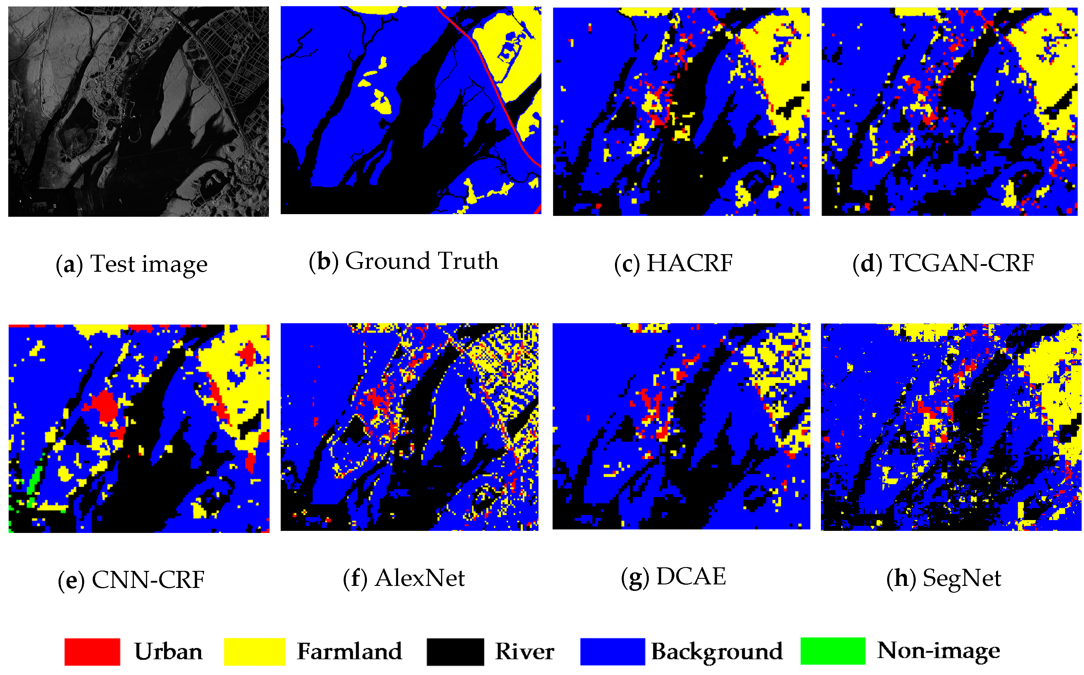
The SAR image in Figure 8a mainly includes rivers and a small amount of farmland. The outline of the rivers is complex and the width of the rivers varies greatly, which increases the difficulty of the segmentation. In the result of the HACRF (Figure 8c), the farmland areas in the upper right corner and the river areas with a large width are completely segmented. What should be noted is that, due to the use of superpixels as the segmentation units, some rivers whose width is less than the superpixels’ width are misclassified as the background. For the TCGAN-CRF (Figure 8d) and CNN-CRF (Figure 8e), it is obvious that there are more superpixels in the central region of the input being misclassified.
5. Discussion
The difference between segmentation and classification tasks is that the segmentation methods need to consider the appearance and spatial consistency. The previous superpixel-wise CRF-based segmentation methods only consider the appearance and spatial consistency in the label optimization stage and they heavily depend on the labeled data. We hope to improve the segmentation performance by taking neighborhood consistency into account in the feature extraction stage and well use the abundant unlabeled samples in training the deep feature extractor.
To verify the effectiveness of our improvements, we finish a series of comparison experiments with some state-of-the-art algorithms. Among them, TCGAN-CRF only utilizes an original CGAN to extract features without considering the relation between the central superpixels and their surrounding superpixels. Its segmentation results are better than the superpixel-wise CNN-CRF method, which uses the common supervised CNN to extract the features of the superpixels. It proves that the introduction of the unlabeled samples in the adversarial training of the CGAN indeed improves the quality of feature extraction and achieves better segmentation performance. Compared with the TCGAN-CRF, our hierarchical CGAN considers the centered superpixels and corresponding background areas during feature extraction. This improvement is consistent with the cognitive laws of human beings. In the absence of background information, it is difficult to judge the classes of the centered superpixel. The background and the target features from the hierarchical CGAN allow us to optimize the training of CRFs. A series of experiments have confirmed that this improvement led to a better OA value, f1 score, and Kappa coefficients in the segmentation results.
We compare the computational time of the proposed method with that of the state-of-the-art methods in Table 5. The running time of our method, TCGAN-CRF and CNN-CRF includes the time for over-segmentation, feature extraction and CRF-based label optimization. Due to the calculation of the distance between adjacent superpixels in the feature space when modeling the CRF, three models have similar computational efficiency. DCAE requires a lot of operations in the Gabor and GLCM feature extraction stages, so it takes the longest time. Since over-segmentation is not needed, AlexNet has the minimal running time.
SegNet is a commonly used end-to-end supervised deep segmentation method. It has a common encoder–decoder structure used in pixel-level semantic segmentation networks. It employs the convolution layers to learn the texture features, and uses subsequent deconvolution operations to learn the spatial distribution of all the pixels. Our method achieves better segmentation performance over SegNet. The use of deconvolution shows that the SegNet can only achieve pixel-level segmentation, which brings a larger computation burden. Hence its running time is comparable to that of the DCAE.
In short, our approach introduces conditional adversarial networks to learn information from the unlabeled samples and lessen the reliance on the labeled samples. Both the target and background features are extracted by the hierarchical CGANs for CRF-based optimization. The above two improvements make our segmentation accuracy better than the other methods. The weakness of our approach is that it is not an end-to-end method, and the training of the feature extraction part and CRF is carried out differently.
In future research, we will unify CRF parameter learning and feature extractor learning into one network to facilitate the end-to-end segmentation. Although pixel-level segmentation with CNNs and CRF has been implemented in [40,41], the positional relation between the neighboring superpixels in the superpixel-wise segmentation algorithms is too complex.
6. Conclusions
In this study, a new segmentation algorithm combining hierarchical CGANs with CRF has been presented for high-resolution airborne SAR imagery. The original images are first over-segmented into the initial superpixels. Then, we design a hierarchical CGANs network to extract the feature vectors of the superpixels. On the one hand, the introduction of CGAN enables this network to learn its parameters using the unlabeled samples. The experiments for feature extraction analysis show the CGAN can improve the separability of the features of individual classes, and thus facilitate better segmentation results. On the other hand, inspired by the cognitive laws of human beings, this network simultaneously extracts the feature vectors of the centered superpixels and their corresponding background areas. The addition of the background information allows us to obtain optimal unary and pairwise potential parameters in CRF models and effectively preserve the neighbor consistency in the segmentation results. Evaluation measures on the datasets also show that this method further improves the segmentation accuracy.
Author Contributions
Conceptualization, F.M.; Methodology, F.G. and F.M.; Software, F.G.; Validation, J.S. and A.H.; Resources, J.S. and A.H.; Writing-Original Draft Preparation, F.M.; Writing-Review & Editing, F.G., A.H. and H.Z.; Visualization, H.Z.; Supervision, F.G. and H.Z.; Project Administration, F.G.; Funding Acquisition, F.G., F.M., A.H. and H.Z.
Funding
This research was funded by the National Natural Science Foundation of China, grant nos. 61771027, 61071139, 61471019, 61501011, and 61171122. Fei Ma was supported by Academic Excellence Foundation of BUAA for PhD Students. H. Zhou was supported by UK EPSRC under Grant EP/N011074/1, Royal Society-Newton Advanced Fellowship under Grant NA160342, and European Union’s Horizon 2020 research and innovation program under the Marie-Sklodowska-Curie grant agreement no. 720325. Professor A. Hussain was supported by the UK Engineering and Physical Sciences Research Council (EPSRC) grant no. EP/M026981/1.
Acknowledgments
The SAR images used in the experiments are the courtesy of Beijing Institute of Radio Measurement, the authors would like to thank them for their support in this work.
Conflicts of Interest
The authors declare no conflict of interest.
References
- Mason, D.; Davenport, I.; Neal, J.; Schumann, G.; Bates, P.D. Nearreal-time flood detection in urban and rural areas using high resolution synthetic aperture radar images. IEEE Trans. Geosci. Remote Sens. 2012, 50, 3041–3052. [Google Scholar] [CrossRef]
- Covello, F.; Battazza, F.; Coletta, A.; Lopinto, E.; Fiorentino, C.; Pietranera, L.; Valentini, G.; Zoffoli, S. COSMO-SkyMed—An existing opportunity for observing the Earth. J. Geodyn. 2010, 49, 171–180. [Google Scholar] [CrossRef]
- Prati, C.M.; Rocca, F.; Asaro, F.; Belletti, B.; Bizzi, S. Use of cross-POL multi-temporal SAR data for image segmentation. In Proceedings of the 2018 IEEE International Conference on Environmental Engineering, Milan, Italy, 12–14 March 2018; pp. 1–6. [Google Scholar]
- Zhou, L.; Guo, C.; Li, Y.; Shang, Y. Change Detection Based on Conditional Random Field with Region Connection Constraints in High-Resolution Remote Sensing Images. IEEE J. Sel. Top. Appl. Earth Obs. Remote Sens. 2017, 9, 3478–3488. [Google Scholar] [CrossRef]
- Suykens, J.A.K.; Vandewalle, J. Least squares support vector machine classifiers. Neural Process. Lett. 1999, 9, 293–300. [Google Scholar] [CrossRef]
- Liaw, A.; Wiener, M. Classification and regression by random Forest. R News 2002, 2, 18–22. [Google Scholar]
- Wright, J.; Yang, A.Y.; Ganesh, A.; Sastry, S.S.; Ma, Y. Robust face recognition via sparse representation. IEEE Trans. Pattern Anal. Mach. Intell. 2009, 31, 210–227. [Google Scholar] [CrossRef] [PubMed]
- Lang, F.; Yang, J.; Yan, S.; Qin, F. Superpixel Segmentation of Polarimetric Synthetic Aperture Radar (SAR) Images Based on Generalized Mean Shift. Remote Sens. 2018, 10, 1592. [Google Scholar] [CrossRef]
- Stutz, D.; Hermans, A.; Leibe, B. Superpixels: An Evaluation of the State-of-the-Art. Comput. Vis. Image Underst. 2018, 166, 1–27. [Google Scholar] [CrossRef]
- Ciecholewski, M. River channel segmentation in polarimetric SAR images. Expert Syst. Appl. 2017, 82, 196–215. [Google Scholar] [CrossRef]
- Cousty, J.; Bertrand, G.; Najman, L.; Couprie, M. Watershed cuts: Thinnings, shortest path forests, and topological watersheds. IEEE Trans. Pattern Anal. Mach. Intell. 2010, 32, 925–939. [Google Scholar] [CrossRef] [PubMed]
- Braga, A.M.; Marques, R.C.P.; Rodrigues, F.A.A.; Medeiros, F.N.S. A Median Regularized Level Set for Hierarchical Segmentation of SAR Images. IEEE Geosci. Remote Sens. Lett. 2017, 14, 1171–1175. [Google Scholar] [CrossRef]
- Jin, R.; Yin, J.; Zhou, W.; Jian, Y. Level Set Segmentation Algorithm for High-Resolution Polarimetric SAR Images Based on a Heterogeneous Clutter Model. IEEE J. Sel. Top. Appl. Earth Obs. Remote Sens. 2017, 10, 4565–4579. [Google Scholar] [CrossRef]
- Lafferty, J.D.; Mccallum, A.; Pereira, F.C.N. Conditional Random Fields: Probabilistic Models for Segmenting and Labeling Sequence Data. In Proceedings of the 18th International Conference on Machine Learning 2001 (ICML 2001), Williamstown, WA, USA, 28 June–1 July 2001; Volume 3, pp. 282–289. [Google Scholar]
- Liu, F.; Lin, G.; Shen, C. CRF learning with CNN features for image segmentation. Pattern Recognit. 2015, 48, 2983–2992. [Google Scholar] [CrossRef]
- Szummer, M.; Kohli, P.; Hoiem, D. Learning CRFs Using Graph Cuts. In Proceedings of the European Conference on Computer Vision, Marseille, France, 12–18 October 2008. [Google Scholar]
- Zhong, P.; Wang, R. Learning conditional random fields for classification of hyperspectral images. IEEE Trans. Image Process. 2010, 19, 1890–1907. [Google Scholar] [CrossRef] [PubMed]
- Xu, L.; Clausi, D.A.; Li, F.; Wong, A. Weakly Supervised Classification of Remotely Sensed Imagery Using Label Constraint and Edge Penalty. IEEE Trans. Geosci. Remote Sens. 2017, 55, 1424–1436. [Google Scholar] [CrossRef]
- Sultani, W.; Mokhtari, S.; Yun, H.B. Automatic Pavement Object Detection Using Superpixel Segmentation Combined with Conditional Random Field. IEEE Trans. Intell. Transp. Syst. 2018, 19, 2076–2085. [Google Scholar] [CrossRef]
- Li, Y.; Tan, Y. Cauchy Graph Embedding Optimization for Built-Up Areas Detection from High-Resolution Remote Sensing Images. IEEE J. Sel. Top. Appl. Earth Obs. Remote Sens. 2015, 8, 2078–2096. [Google Scholar] [CrossRef]
- Guo, E.; Bai, L.; Zhang, Y.; Han, J. Vehicle Detection Based on Superpixel and Improved HOG in Aerial Images. In International Conference on Image and Graphics; Springer: Cham, Switzerland, 2017. [Google Scholar]
- Xiang, D.; Tang, T.; Zhao, L.; Su, Y. Superpixel Generating Algorithm Based on Pixel Intensity and Location Similarity for SAR Image Classification. IEEE Geosci. Remote Sens. Lett. 2013, 10, 1414–1418. [Google Scholar] [CrossRef]
- Micusik, B.; Kosecka, J. Semantic segmentation of street scenes by superpixel co-occurrence and 3D geometry. In Proceedings of the IEEE International Conference on Computer Vision Workshops, Kyoto, Japan, 27 September–4 October 2009. [Google Scholar]
- Lawrence, S.; Giles, C.L.; Tsoi, A.C.; Back, A.D. Face recognition: A convolutional neural-network approach. IEEE Trans. Neural Netw. 1997, 8, 98–113. [Google Scholar] [CrossRef] [PubMed]
- Chen, H.; Zhang, F.; Tang, B.; Yin, Q.; Sun, X. Slim and Efficient Neural Network Design for Resource-Constrained SAR Target Recognition. Remote Sens. 2018, 10, 1618. [Google Scholar] [CrossRef]
- Gao, F.; Ma, F.; Wang, J.; Sun, J.; Zhou, H. Visual Saliency Modeling for River Detection in High-resolution SAR Imagery. IEEE Access 2018, 6, 1000–1014. [Google Scholar] [CrossRef]
- Liu, F.; Lin, G.; Shen, C. Discriminative Training of Deep Fully-connected Continuous CRFs with Task-specific Loss. IEEE Trans. Image Process. 2017, 26, 2127–2136. [Google Scholar] [CrossRef] [PubMed]
- Alshehhi, R.; Marpu, P.R. Hierarchical graph-based segmentation for extracting road networks from high-resolution satellite images. ISPRS J. Photogramm. Remote Sens. 2017, 126, 245–260. [Google Scholar] [CrossRef]
- Vincent, P.; Larochelle, H.; Lajoie, I.; Bengio, Y.; Manzagol, P.A. Stacked Denoising Autoencoders: Learning Useful Representations in a Deep Network with a Local Denoising Criterion. J. Mach. Learn. Res. 2010, 11, 3371–3408. [Google Scholar]
- Nair, V.; Hinton, G.E. Rectified linear units improve restricted boltzmann machines. In Proceedings of the International Conference on International Conference on Machine Learning, Haifa, Israel, 21–24 June 2010. [Google Scholar]
- Bengio, Y.; Lamblin, P.; Dan, P.; Larochelle, H. Greedy layer-wise training of deep networks. Adv. Neural Inf. Process. Syst. 2007, 19, 153–160. [Google Scholar]
- Goodfellow, I.J.; Pouget-Abadie, J.; Mirza, M.; Bing, X.; Warde-Farley, D.; Ozair, S.; Courville, A.; Bengio, Y. Generative adversarial nets. In Proceedings of the International Conference on Neural Information Processing Systems, Montreal, QC, Canada, 8–13 December 2014. [Google Scholar]
- Varia, N.; Dokania, A.; Senthilnath, J. DeepExt: A Convolution Neural Network for Road Extraction using RGB images captured by UAV. In Proceedings of the 2018 IEEE Symposium Series on Computational Intelligence (SSCI), Bangalore, India, 18–21 November 2018; pp. 1890–1895. [Google Scholar]
- Fei, G.; Fei, M.; Wang, J.; Sun, J.; Yang, E.; Zhou, H. Semi-Supervised Generative Adversarial Nets with Multiple Generators for SAR Image Recognition. Sensors 2018, 18, 2706. [Google Scholar]
- Chen, L.C.; Papandreou, G.; Kokkinos, I.; Murphy, K.; Yuille, A.L. Semantic Image Segmentation with Deep Convolutional Nets and Fully Connected CRFs. Comput. Sci. 2014, 4, 357–361. [Google Scholar]
- Achanta, R.; Shaji, A.; Smith, K.; Lucchi, A.; Fua, P.; Süsstrunk, S. SLIC Superpixels Compared to State-of-the-Art Superpixel Methods. IEEE Trans. Pattern Anal. Mach. Intell. 2012, 34, 2274–2282. [Google Scholar] [CrossRef] [PubMed]
- Kenduiywo, B.K.; Bargiel, D.; Soergel, U. Higher Order Dynamic Conditional Random Fields Ensemble for Crop Type Classification in Radar Images. IEEE Trans. Geosci. Remote Sens. 2017, 55, 4638–4654. [Google Scholar] [CrossRef]
- Geng, J.; Fan, J.; Wang, H.; Ma, X.; Li, B.; Chen, F. High-Resolution SAR Image Classification via Deep Convolutional Autoencoders. IEEE Geosci. Remote Sens. Lett. 2015, 12, 1–5. [Google Scholar] [CrossRef]
- Csillik, O. Fast Segmentation and Classification of Very High Resolution Remote Sensing Data Using SLIC Superpixels. Remote Sens. 2017, 9, 243. [Google Scholar] [CrossRef]
- Zheng, S.; Jayasumana, S.; Romera-Paredes, B.; Vineet, V.; Su, Z.; Du, D.; Huang, C.; Torr, P.H. Conditional Random Fields as Recurrent Neural Networks. In Proceedings of the IEEE International Conference on Computer Vision (ICCV), Santiago, Chile, 13–16 December 2015. [Google Scholar]
- Lin, G.; Shen, C.; Hengel, A.V.D.; Reid, I. Efficient Piecewise Training of Deep Structured Models for Semantic Segmentation. In Proceedings of the IEEE Conference on Computer Vision and Pattern Recognition (CVPR), Las Vegas, NV, USA, 26 June–1 July 2016; pp. 3194–3203. [Google Scholar]
- Salimans, T.; Goodfellow, I.; Zaremba, W.; Cheung, V.; Radford, A.; Chen, X. Improved Techniques for Training GANs. In Proceedings of the Advances in Neural Information Processing Systems (NIPS 2016), Barcelona, Spain, 5–10 December 2016; pp. 2234–2242. [Google Scholar]
- Martins, A.F.T.; Figueiredo, M.A.T.; Aguiar, P.M.Q.; Smith, N.A.; Xing, E.P. AD3: Alternating directions dual decomposition for map inference in graphical models. J. Mach. Learn. Res. 2015, 16, 495–545. [Google Scholar]
- Zhang, F.; Yao, X.; Tang, H.; Yin, Q.; Hu, Y.; Lei, B. Multiple Mode SAR Raw Data Simulation and Parallel Acceleration for Gaofen-3 Mission. IEEE J. Sel. Top. Appl. Earth Obs. Remote Sens. 2018, 11, 2115–2126. [Google Scholar] [CrossRef]
- Martha, T.R.; Kerle, N.; Westen, C.J.V.; Jetten, V.; Kumar, K.V. Segment Optimization and Data-Driven Thresholding for Knowledge-Based Landslide Detection by Object-Based Image Analysis. IEEE Trans. Geosci. Remote Sens. 2011, 49, 4928–4943. [Google Scholar] [CrossRef]
- Jie, G.; Wang, H.; Fan, J.; Ma, X. SAR Image Classification via Deep Recurrent Encoding Neural Networks. IEEE Trans. Geosci. Remote Sens. 2018, 56, 2255–2269. [Google Scholar]
- Sasaki, Y. The truth of the F-measure. Teach. Tutor Mater. 2007, 1, 1–5. [Google Scholar]
- Cohen, J. A coefficient of agreement for nominal scales. Educ. Psychol. Meas. 1960, 20, 37–46. [Google Scholar] [CrossRef]
- Xu, B.; Wang, N.; Chen, T.; Li, M. Empirical Evaluation of Rectified Activations in Convolutional Network. arXiv, 2015; arXiv:1505.00853. [Google Scholar]
- Wold, S. Principal component analysis. Chemom. Intell. Lab. Syst. 1987, 2, 37–52. [Google Scholar] [CrossRef]
- Krizhevsky, A.; Sutskever, I.; Hinton, G.E. ImageNet classification with deep convolutional neural networks. In Proceedings of the International Conference on Neural Information Processing Systems, Lake Tahoe, NV, USA, 3–6 December 2012. [Google Scholar]
- Deng, J.; Dong, W.; Socher, R.; Li, L.J.; Li, K.; Fei-Fei, L. ImageNet: A large-scale hierarchical image database. In Proceedings of the IEEE Conference on Computer Vision & Pattern Recognition, Miami, FL, USA, 20–25 June 2009. [Google Scholar]
- Badrinarayanan, V.; Kendall, A.; Cipolla, R. SegNet: A Deep Convolutional Encoder-Decoder Architecture for Image Segmentation. arXiv, 2015; arXiv:1505.07293. [Google Scholar]
- Tian, T.; Chang, L.; Jinkang, X.; Ma, J. Urban Area Detection in Very High Resolution Remote Sensing Images Using Deep Convolutional Neural Networks. Sensors 2018, 18, 904. [Google Scholar] [CrossRef] [PubMed]
- Ren, S.; He, K.; Girshick, R.; Sun, J. Faster R-CNN: Towards real-time object detection with region proposal networks. In Proceedings of the International Conference on Neural Information Processing Systems, Montreal, QC, Canada, 7–12 December 2015. [Google Scholar]
Figure 1.
Architecture of our weakly supervised segmentation method based on HACRF.

Figure 2.
The architecture of the hierarchical CGAN, consisting of a target CGAN(TCGAN) and a background CGAN(BCGAN). In the training stage, the target superpixels and background superpixels are respectively utilized to train TCGAN and BCGAN.
Figure 2.
The architecture of the hierarchical CGAN, consisting of a target CGAN(TCGAN) and a background CGAN(BCGAN). In the training stage, the target superpixels and background superpixels are respectively utilized to train TCGAN and BCGAN.

Figure 3.
Part of images and the corresponding ground truth.

Figure 4.
The parameters of TCGAN. The generator (blue rectangles) is composed of FC block 1, FC block 2, deconv block 1, and deconv block 2. The T-feature extractor (red rectangles) consists of the convolution block 1 and the fully-connected block 3. The Discriminator block and Multi-Classifier block are both implemented by a fully-connected layer.

Figure 5.
Visualization the features extracted from some testing images using individual methods. (a) HACRF; (b) CGAN; (c) CNN; (d) AlexNet; (e) DCAE.
Figure 5.
Visualization the features extracted from some testing images using individual methods. (a) HACRF; (b) CGAN; (c) CNN; (d) AlexNet; (e) DCAE.

Figure 6.
Comparison of the pixel-wise precision and recall for individual classes of superpixels with five state-of-the-art algorithms. (a) pixel-wise precision; (b) pixel-wise recall.
Figure 6.
Comparison of the pixel-wise precision and recall for individual classes of superpixels with five state-of-the-art algorithms. (a) pixel-wise precision; (b) pixel-wise recall.

Figure 7.
Segmentation results of six models on FangChengGang dataset. (a) Input image; (b) ground truth; (c) HACRF; (d) TCGAN-CRF; (e) CNN-CRF; (f) AlexNet; (g) DCAE; (h) SegNet.
Figure 7.
Segmentation results of six models on FangChengGang dataset. (a) Input image; (b) ground truth; (c) HACRF; (d) TCGAN-CRF; (e) CNN-CRF; (f) AlexNet; (g) DCAE; (h) SegNet.

Figure 8.
Segmentation results of six models on FangChengGang dataset. (a) Input image; (b) ground truth; (c) HACRF; (d) TCGAN-CRF; (e) CNN-CRF; (f) AlexNet; (g) DCAE; (h) SegNet.
Figure 8.
Segmentation results of six models on FangChengGang dataset. (a) Input image; (b) ground truth; (c) HACRF; (d) TCGAN-CRF; (e) CNN-CRF; (f) AlexNet; (g) DCAE; (h) SegNet.


Table 1.
Compared recently CRF-based segmentation in terms of pros and cons.
| Models | Benefits | Defect |
|---|---|---|
| Pixel-wise CRF [16,35] | --- | Heavy calculation burden |
| Superpixel-wise + hand crafted feature + CRF [19,37] | Unsupervised; fewer calculation | Parameters designed by experiences |
| Superpixel-wise + deep feature + CRF [15,19,39] | Outstanding feature extraction ability | Supervised |
| End-to-end deep CRF [40,41] | Compact construction | Supervised |
Table 2.
The numbers of superpixels of diverse classes in the training and testing set.
| Urban | Farmland | River | Background | Non-Image | |
|---|---|---|---|---|---|
| Train | 6825 | 7332 | 7164 | 27,724 | 7402 |
| Test | 13,822 | 10,546 | 29,293 | 136,418 | 44,019 |
| Percent | 33.06% | 41.01% | 19.85% | 16.89% | 14.39% |
Table 3.
Comparison of the overall segmentation performance with five state-of-the-art methods.
| HACRF | TCGAN-CRF | CNN-CRF | AlexNet | DCAE | SegNet | |
|---|---|---|---|---|---|---|
| OP (%) | 86.93 | 85.28 | 81.68 | 77.29 | 78.78 | 85.85 |
| OA (%) | 85.82 | 83.59 | 78.97 | 76.15 | 79.75 | 84.90 |
| F1-score (%) | 86.09 | 84.07 | 79.68 | 76.51 | 79.08 | 85.16 |
| κ | 0.7736 | 0.7418 | 0.6752 | 0.6303 | 0.6725 | 0.7579 |
Table 4.
Comparison of the pixel-wise F1 scores for individual classes with five state-of-the-art methods.
Table 4.
Comparison of the pixel-wise F1 scores for individual classes with five state-of-the-art methods.
| Class | HACRF | TCGAN-CRF | CNN-CRF | AlexNet | DCAE | SegNet |
|---|---|---|---|---|---|---|
| Urban | 63.17 | 56.72 | 62.54 | 45.79 | 54.86 | 61.46 |
| Farmland | 70.63 | 63.08 | 50.42 | 25.12 | 27.89 | 52.56 |
| River | 73.67 | 72.76 | 57.25 | 70.15 | 71.01 | 75.00 |
| Background | 88.10 | 86.13 | 85.16 | 80.69 | 83.79 | 90.43 |
| Non-image | 99.48 | 99.42 | 90.53 | 98.92 | 98.33 | 99.04 |
Table 5.
Comparison of run time (seconds) with five state-of-the-art algorithms.
| Class | HACRF | TCGAN-CRF | CNN-CRF | AlexNet | DCAE | SegNet |
|---|---|---|---|---|---|---|
| Time(s) | 2183.15 | 2207.05 | 2775.87 | 480.34 | 4219.64 | 3379.75 |
© 2019 by the authors. Licensee MDPI, Basel, Switzerland. This article is an open access article distributed under the terms and conditions of the Creative Commons Attribution (CC BY) license (http://creativecommons.org/licenses/by/4.0/).
Share and Cite
MDPI and ACS Style
Ma, F.; Gao, F.; Sun, J.; Zhou, H.; Hussain, A. Weakly Supervised Segmentation of SAR Imagery Using Superpixel and Hierarchically Adversarial CRF. Remote Sens. 2019, 11, 512. https://doi.org/10.3390/rs11050512
AMA Style
Ma F, Gao F, Sun J, Zhou H, Hussain A. Weakly Supervised Segmentation of SAR Imagery Using Superpixel and Hierarchically Adversarial CRF. Remote Sensing. 2019; 11(5):512. https://doi.org/10.3390/rs11050512
Chicago/Turabian StyleMa, Fei, Fei Gao, Jinping Sun, Huiyu Zhou, and Amir Hussain. 2019. "Weakly Supervised Segmentation of SAR Imagery Using Superpixel and Hierarchically Adversarial CRF" Remote Sensing 11, no. 5: 512. https://doi.org/10.3390/rs11050512
Note that from the first issue of 2016, this journal uses article numbers instead of page numbers. See further details here.