Radiance Uncertainty Characterisation to Facilitate Climate Data Record Creation


1
National Centre for Earth Observation and Department of Meteorology, University of Reading, Reading RG6 6AL, UK
2
Department of Meteorology, University of Reading, Reading RG6 6AL, UK
3
National Physical Laboratory, Teddington TW11 0LW, UK
*
Author to whom correspondence should be addressed.
Remote Sens. 2019, 11(5), 474; https://doi.org/10.3390/rs11050474
Submission received: 12 February 2019
/
Accepted: 16 February 2019
/
Published: 26 February 2019
(This article belongs to the Special Issue Assessment of Quality and Usability of Climate Data Records)
Abstract
:The uncertainty in a climate data records (CDRs) derived from Earth observations in part derives from the propagated uncertainty in the radiance record (the fundamental climate data record, FCDR) from which the geophysical estimates in the CDR are derived. A common barrier to providing uncertainty-quantified CDRs is the inaccessibility to CDR creators of appropriate radiance uncertainty information in the FCDR. Here, we propose radiance uncertainty information designed directly to facilitate estimation of propagated uncertainty in derived CDRs at full resolution and in gridded products. Errors in Earth observations are typically highly structured and complex, and the uncertainty information we propose is of intermediate complexity, sufficient to capture the main variability in propagated uncertainty in a CDR, while avoiding unfeasible complexity or data volume. The uncertainty and error correlation characteristics of uncertainty are quantified for three classes of error with different propagation properties: independent, structured and common radiance errors. The meaning, mathematical derivations, practical evaluation and example applications of this set of uncertainty information are presented.
1. Introduction
Climate data records (CDRs) are generated from Earth observations within several programmes [1,2,3,4] in support of societal and scientific needs to quantify change and variability in Earth’s climate system. The uncertainty in the trends and variations of climate variables in CDRs is arguably as important to understand as the trends and variations themselves, in order to avoid incorrect inferences or optimistic levels of confidence in conclusions drawn from the data [5,6,7,8]. Recently, greater efforts have been directed to CDR generation [9,10], and specifically to quantifying uncertainty in CDRs [11,12,13]. Consideration has been given to good practice, drawing on experience across a range of essential climate variables [14], a major conclusion being that in cases where uncertainty in the CDR is highly variable, uncertainty evaluations should be available per datum. This implies the need to understand and model the dominant processes causing uncertainty in the CDR.
Climate data records from Earth observation are derived by a series of transformations of data. Raw telemetry is processed by a ground segment to ‘level-1’ datasets, comprising radiances or counts with sufficient information to convert to calibrated radiances. Note that radiances may then be expressed as brightness temperature or reflectance in level-1 products, and in this paper, we use “radiance” generically to encompass all such quantities. It also needs to be acknowledged that some level-1 data comprise signals of a different nature, as in the cases of altimetry and gravimetry. In level-1 data, observations are also located in time and space. A level-1 dataset of sufficient length, consistency and stability to support the derivation of a CDR may be referred to as a fundamental climate data record (FCDR). From the level-1 dataset, often using retrieval techniques involving multi-channel inferences, estimates of geophysical quantities are derived, and the full resolution dataset of the retrieved variable is described as a CDR at ‘level 2’. For some applications, regularly gridded data are preferred, often at a lower spatio-temporal resolution, and level-2 data may be averaged on such a regular grid to generate a CDR at ‘level-3’. Further processing to other forms of higher-level dataset may also be done.
At each transformation from level 1 to level 3 and beyond, there is both (i) propagation of uncertainty from the lower-level data to the higher, and (ii) introduction of new sources of uncertainty by virtue of the parameters, assumptions and/or limitations of the method of data transformation [15]. The relative importance of these two sources of uncertainty in a CDR will vary, depending on the nature of the radiance data and of the retrieval process. Generally, rigorously quantifying CDR uncertainty requires propagation of radiance uncertainty through the transformations to higher levels.
In practice, a large proportion of level-1/FCDR datasets contain either no or very limited radiance uncertainty information, meaning that CDR creators have no practical means to evaluate propagated radiance uncertainty. In part, this situation arises because it is not obvious what selection of radiance uncertainty information is needed to adequately support CDR creation, given that providing comprehensive uncertainty information would entail infeasible data volumes and/or complexity (see below).
The focus of this paper is to address the question, “What radiance uncertainty information should be provided to support the characterisation of uncertainty in derived CDRs?” The proposed approach is intended to support propagation of uncertainty to levels 2 and 3, which means that inter-channel and spatio-temporal error correlations must be included. The key contributions of the paper are (i) to propose a set of summary information on errors and their correlations that it is feasible and sufficient to provide, and (ii) to summarise the mathematics and computing techniques required to calculate this uncertainty information. References [15,16,17,18,19] illustrate the working out of these concepts in particular cases.
Although facilitating CDR generation is our focus, we note that radiance uncertainty information at level 1 is also directly relevant to environmental re-analysis using data assimilation e.g., [20]. In data assimilation, the ideal approach is to assimilate level-1 observations. An evaluation of the observation-to-model error covariance associated with FCDRs is required by the assimilation, and the observation-related component of this is directly addressed by the methods described in this paper. Data assimilation may also help validate uncertainty information in FCDRs and CDRs [21], although this topic is beyond the present scope.
The remainder of the paper proceeds as follows. In Section 2, we describe the steps a CDR creator would want to be able to take to propagate and quantify radiance uncertainty in their CDR. From these steps, we infer the uncertainty information that should be provided at level 1 in an FCDR. In Section 3, we outline the understanding necessary to be able to characterise the radiance uncertainty in a single datum, based on understanding sources of error in the instrument. We emphasise that CDR creators should not need such detailed knowledge of the instrument: providing quantification and understanding of level-1 uncertainty should be the responsibility of space agencies, in our view. In Section 4, we present the theory and formulae for turning knowledge of per-datum instrument uncertainty into summary uncertainty information suitable for inclusion in FCDRs, ready for CDR creators to use. Practical evaluation of the formulae requires care, and so these considerations are presented in Section 5. Section 6 briefly illustrates what results can look like in a real case without extensive discussion of the sensor or error sources addressed; this section focuses on the meaning and interpretation of the uncertainty information shown. The concluding Section 7 includes summational remarks regarding the assumptions and implications of the ideas presented, as well as some closing discussion.
2. Requirements for Propagation of Uncertainty to a Climate Data Record
Typically, estimation of a geophysical variable for inclusion in a CDR (i.e., at level-2/3) involves several pre-processing steps followed by a multi-channel retrieval (inference of the variable’s value from a combination of radiance values at different wavelengths). The pre-processing steps may include pixel classification (including target selection or cloud screening) and selection of the valid channel set for the retrieval (which may vary between day and night scenes, for example). In the retrieval step that is applied to the selected pixels, a set of observations is exploited to infer a geophysical variable, . In creating a level-2 CDR, this process of inference usually operates on single pixels. Let the retrieval be
where is the retrieval function which may or may not be expressible analytically, and is the set of retrieval parameters used (which may include externally sourced information). The term obviously does not change the retrieved value , but is explicitly included here to remind us that there are three components to the uncertainty in the retrieved value:
- The propagation of radiance uncertainty through to .
- The propagation of parameter uncertainty through to .
- The uncertainty, “”, introduced into by any approximations and inherent ambiguities of the retrieval that are not directly traceable from uncertainty in or .
This paper is concerned with methods to make the first component listed above straightforward for creators of CDRs to calculate, by defining the uncertainty characterisation that they need.
The propagated radiance standard uncertainty can readily be calculated for a given set of radiances if the radiance error covariance matrix, , is known:
where . Equation (2) is the law of propagation of uncertainty [22], which expresses (i) a first-order approximation in which a small error in, say, propagates linearly to an error in in proportion to the derivative , and (ii) that independent errors combine as the sum of squares. Readers unfamiliar with the matrix form of (2) can readily verify that in the case where is diagonal it corresponds to a textbook expression that may be more familiar: . The matrix form additionally allows for the convenient propagation of correlated errors through any off-diagonal terms in . An off-diagonal term takes the value , where is the correlation coefficient of errors arising between radiance in channels and . When errors are independent, for all , and the error covariance matrix is diagonal.
The answer to the question of this paper, “What radiance uncertainty information should be provided to support the characterisation of uncertainty in derived CDRs?”, thus might seem quite simple: “Provide the radiance error covariance matrix”.
If we assume that it is understood how to estimate for a given set of radiances, there remains a practical problem with this answer: is not a constant matrix. The radiance uncertainty typically arises from several error-causing effects, the relative importance of which may change with instrument state and with the scene characteristics. The degree of cross-channel error correlation is also likely to differ between effects. Thus, the uncertainties, , and the correlation structures, , usually vary. On the other hand, it is not practical and affordable to provide per pixel from the point of view of data volumes [14]. Thus, there is a need to find a useful and efficient approximate representation, preferably one that reflects most of the variability in . That need is addressed in this paper.
Turning to level-3 CDRs, a gridded CDR can generally be considered to contain weighted combinations, , of selected retrieved values,, from the full resolution CDR:
The process of selecting which pixels contribute to includes identifying which pixels lie within the required space-time cell for a given level-3 datum, and perhaps a process to select the best pixels to include. The parameters, , may include weights, length-scales, correlation coefficients, etc. As at level 2, there are three categories of uncertainty in :
- The propagation of retrieved-value uncertainty through to .
- The propagation of gridding parameter uncertainty through to .
- The uncertainty, , introduced by incomplete sampling across the space-time domain which the level-3 datum represents [23]. The uncertainty from incomplete sampling is sometimes referred to as “standard error in the mean”, and reflects observations errors, geophysical variability within the space-time cell, and correlations in these.
Depending on the nature and assumptions of the gridding, the gridding parameter uncertainty, the second bullet above may be justifiably neglected. For example, if the aim is to average evenly across the cell area and the fields of view of the contributing pixels are well quantified, then the weight of each pixel in the cell average may be determined with negligible uncertainty.
Consider the propagation of the retrieved-value uncertainty at pixel level to the cell-mean value. The propagated standard uncertainty is:
where the sensitivity coefficients are now , and is the error covariance matrix of the selected pixels being averaged within the cell. Continuing to assume that the retrieved values are derived one-pixel-at-a-time, what is the structure of ? The simplest possibility arises if the errors in the retrieved pixels are independent, in which case is diagonal and the uncertainty in the cell average diminishes as the familiar . This is rarely, if ever, the case. Retrieval parameters are likely to be strongly related for nearby pixels, and generally so too will be their errors. Noise may be the largest uncertainty in radiances, and although noise may often be independent between pixels, the noise frequency spectrum can be such that there is inter-pixel error correlation [24]. On-board calibration cycles for imagers are once-per-scan-line or less frequent, and calibration errors are correlated across scans and across the duration of the calibration cycle. Error correlations mean that the uncertainty will be greater than the uncertainty expected on the basis of “”. Making a robust estimate of the level-3 uncertainty requires knowledge of error covariance between retrieved values across the cell (level 2), which in turn is in part determined by spatial error covariance in level-1 radiances—i.e., by cross-pixel correlations in radiance errors.
In summary, for propagation of radiance uncertainty to the CDR at level 2 and level 3, estimates of cross-channel and cross-pixel error covariance are needed, and should be available as part of the FCDR. The next two sections briefly describe how such summary error covariance information can be developed from an understanding of the sensor.
3. Methods 1—Radiance Uncertainty Analysis
There are various sources of information from which a good understanding of radiance uncertainty can be developed. Satellite sensors are extensively analysed during design, build and pre-flight characterisation [24]. On-board calibration systems provide information that enables quantification of sensor noise and related calibration uncertainty [25,26], as well as characterisation of the noise spectrum and cross-pixel error correlation [18]. Specifications and pre-flight characterisation of sensor features such as calibration of target properties [26], detector non-linearity [27], sensitivity to instrument temperatures [28] or quantisation [29,30] can be used to infer estimates of uncertainty in the calculated radiance from a range of sources of errors. These are general comments, and it is beyond the scope here to give a comprehensive account of the sources of information that underpin an uncertainty analysis of radiance for a given sensor or sensors in general. A lengthier account of principles of uncertainty analysis applied to Earth observation radiances, with examples, is presented in [15].
The focus of this paper is to show how the outcome of such an uncertainty analysis can be condensed into summary information about radiance uncertainty that is then useful in CDR development. For the sake of argument, therefore, we assume that an uncertainty analysis has been undertaken for a given sensor, resulting in quantification of an adequately comprehensive set of sources of error (“effects”), which will be indexed as . Let the radiance in a given channel, , for a certain pixel, , be calculated as
where is one of the input quantities that appear in the calculation of the FCDR radiance, such as sensor counts, calibration target counts, calibration parameters and measurements of instrument state. The function is the measurement function for radiance. Quantification of an effect, , means that we:
- have identified which input quantity (index ) in the radiance measurement function the effect influences;
- can evaluate the corresponding standard uncertainty associated with that input quantity, which may be a constant for all , may change for every , or be in-between these extremes;
- can estimate the correlation in error in between any pair of channels ; this correlation will usually lie between 1, where the same value of is used in the measurement equation for both channels, and 0, where the values are independent;
- can estimate the error correlation in error in between any pair of pixels of the image in a given channel; and
- can quantify (the sensitivity coefficient of the measurand to the input quantity), either analytically or by perturbation.
Once this set of information has been developed across the key error-causing effects, the required radiance uncertainty information can be calculated, as derived in the next section of this paper.
Here, we now define how the information listed above, i.e., the result of radiance uncertainty analysis, is encapsulated quantitatively, in various matrices.
First, we define the identity matrix, , and the matrix of ones, . The former describes the error correlation between quantities that are independent. The latter describes the error correlation between quantities subject to errors that are in common (or in fixed proportions). We have:
Second, we introduce notation for error correlation matrices. There are several such matrices that we will need to distinguish carefully, and thus the notation is necessarily detailed. All error correlation matrices will be represented as . The subscripts and superscripts have meanings according to their position, as follows.
- is an index across a dimension of the satellite image, and indicates the dimension across which the matrix expresses the error correlations. This subscript can take the following values: , the channel dimension, indicating a cross-channel error correlation matrix; , the image element dimension, indicating a cross-element error correlation matrix; , the image line dimension; and , used to index pixels generically (across both lines and elements), as when indexing a selection of pixels within a particular L3 grid-cell.
- The superscripts , etc., identify indices (line, elements, input quantities or effects) over which the matrix does not average or integrate: in the superscript position indicates the error covariance matrix is evaluated for a specific pixel, ; alone means we are referring to evaluation for single pixels generically, without specifying which pixel particularly; in this position indicates that the matrix refers to one specific effect, ; and so on.
- , if present, indicates a sub-set of effects whose combined effect is quantified by the error correlation matrix; absence of this optional label indicates all effects have been combined; the possible sub-sets of effects will be defined in Section 4.
The partition between superscripts and subscripts is, in summary, as follows: the subscripts indicate the aspects the covariance matrix does include, while the superscripts express aspects across which the matrix does not average or integrate.
For example, refers to a cross-channel error correlation matrix (subscript ) for one identified effect, (superscript ), evaluated at a single, arbitrary image pixel, . We use the same labelling convention for corresponding error covariance matrices, such that would designate a cross-pixel error covariance matrix (subscript ) from all effects affecting the th measurement equation input quantity, evaluated for a single, arbitrary image-pixel.
Third, we introduce notation for uncertainty. The uncertainty of the measured value in pixel in channel arising from the combination of all effects is:
where the notation of the summation makes explicit that each input quantity can be affected by more than one effect, hence the double sum over all (effect given input quantity ) and (input quantities). The sensitivity coefficients, , change with the input quantity but not the effect, whereas each effect contributes its own uncertainty, , in the relevant input quantity. All these effects are likely to vary between channels, and may vary across lines and/or elements in the image. Using the same labelling convention as error correlation matrices, the matrix is a diagonal matrix with the diagonal elements calculated across channels, lines, elements or pixels (as indicated by ) for the specific instances indicated by the superscript(s), . For example,
shows an uncertainty matrix with diagonal elements being the uncertainty in the th input quantity arising from one of the effects, , relevant to that input quantity.
Lastly, we define the sensitivity matrix, in a similar way to uncertainty. Thus, for example,
shows a sensitivity matrix of the sensitivities to the th input quantity of the radiance measurement equation across different channels, for a single choice of image line and element.
4. Methods 2—Equations to Define Summary Uncertainty Information
A conclusion of Section 2 was that propagation of radiance uncertainty to the CDR at level 2 and level 3 requires estimates of the cross-channel and cross-pixel error covariances to be provided at level 1. In this section, the equations necessary to quantify these covariances are developed, starting with calculation of the cross-channel error covariance matrix.
Considering a single effect, , at an arbitrary pixel, , in an image, the cross-channel radiance error covariance matrix is equal to:
where is the index of the input quantity in which the effect causes error. The form of this is analogous to the earlier equations for propagation of uncertainty, with the error covariance on the right-hand side (representing the uncertainty that is to be propagated to the radiance) has been decomposed into a diagonal matrix of uncertainty values, , and the error correlation matrix, . The total error covariance matrix from all the analysed effects is the sum of the individual error covariances:
Given the results of radiance uncertainty analysis, this channel covariance matrix could be provided for every pixel, in principle. However, while the radiance data scales as , the matrix scales as , which is impractical for users, since FCDRs are already often multi-terabyte or petabyte datasets. An average estimate can be made and provided, by averaging over an adequate sample of pixels:
where is an operator to average over a sample of pixels. (In line with the nomenclature introduced earlier, the absence of a superscript in indicates that all effects have been combined and that there is averaging over pixels.)
Provision of would be an advance over present practice, but can be further improved to allow CDR producers the ability to reflect some of the variability in uncertainty across an image. (Where data are provided as whole orbits, for example, the instrument state may change and radiance uncertainty may vary significantly.) One approach is to provide, instead of , the average radiance error correlation matrix per image, , which can be combined with a data layer quantifying per pixel uncertainty. The approximation assumed in this approach is that the error correlations are relatively constant, whereas uncertainty significantly changes. Any covariance matrix, being positive definite and symmetric, can be represented in the form . To see this, let element of the matrix, , be , etc. Make the following identifications:
where is zero when and one when . Calculating recovers . This is the principle on which an overall error correlation matrix can be calculated for a combination of effects. Thus, if is the diagonal matrix whose diagonal elements are the square roots of the diagonal elements of , the required average error correlation matrix is:
The use of , combined with uncertainty estimates across the image, will be described later.
The same equations apply to calculating error covariance across elements and lines. For example, the representative cross-element error correlation matrix (for a given channel) is defined by:
and equivalent expressions for cross-line error correlations can be obtained by swapping the and indices. The dimensions of and are, respectively, the squares of the number of along-track lines and the number of elements squared (); this is often likely to represent an impractical additional data volume. If further data reduction is required, the approximation may be made that error correlations vary spatially as a function of element or line separation only, i.e., as a function of and , respectively. If we write, for example, , then the average error correlation value for pixels on a given line separated by a difference in element index equal to can be calculated using:
with a similar equation for the cross-line average error correlation. is a vector containing elements evaluating this equation for pixel separations from (for which ) to . From this, an ‘average’ can be constructed by substituting for .
To summarise the implications of the above mathematical development, methods have been proposed to calculate:
- a representative cross-channel error correlation matrix (affordable volume-wise)
- a representative cross-line error correlation function (from which an approximate error correlation matrix etc can be inferred where the matrix itself is unaffordable volume-wise), and
- a representative cross-element error correlation function
from which all the necessary error covariance matrices for uncertainty propagation to the CDR can be generated using the uncertainty provided for each pixel.
The development above is framed in terms of a single set of uncertainty and error correlations being able to represent all effects. This is a strong approximation and does not enable the correlation structure to respond to relative changes in uncertainty from effects with contrasting error structures. (Such relative changes in uncertainty can arise, for example, when an instrument’s gain changes and the balance of pure noise versus calibration uncertainty may change.)
To lessen the degree of the approximation, we can subdivide effects into families of similar error correlation structure, providing the set of information above for each family. Such a subdivision, of course, increases complexity and data volume, so a balance needs to be struck. A traditional split is to partition “random” and “systematic” error sources. We have found that this is not adequate to describe the errors in a satellite image, because there are important intermediate effects that cause errors that are in common or partially correlated across certain groups of pixels (and thus are neither random nor systematic in the usual sense). The minimum complexity that reflects this situation is a tripartite division of effects. A tripartite approach to uncertainty information has previously been adopted in thermal remote sensing of sea and land surface temperatures at level 2/CDR e.g., [19], and here we discuss how it can also apply at level 1 (and support the tripartite calculations for CDRs).
We categorise each of the effects, , into one subset according to their correlation structure. The set of independent effects, , contains effects where there is no (or negligible) correlation of error between pixels. White noise from statistical fluctuations in detectors or amplifier circuits on the sensor would fall into this category. At the other extreme would be common effects, , which cause the same unknown error in all pixels (at least approximately on some large scale). The uncertainty from common effects can be characterised across an image by a single uncertainty estimate. Between these extremes are structured effects, , which can be either random or systematic in their physical origin, whose defining characteristic is that they cause errors that are partially shared across at least some pixels in the image. This tripartite classification is discussed in detail in [15].
Equations (10) to (15) can all be applied to independent and structured effects separately. For example, the modification of eq. 11 for independent effects is:
which uses the fact that for independent effects by definition. (An extension is made to the notation, with the second subscript, , of indicates the effects class if it is a subset of all.) Covariances may be added, and , while for a particular pixel the total uncertainty is the root sum of squares of the three component uncertainties.
5. Methods 3—Practical Computation
Calculating the “CURUC” equations presented in the previous section can be practically challenging because of the size and number of dimensions of the arrays involved. A literal implementation of the equations with each matrix in its own array is inefficient with regard to computer memory and the number of required floating point operations. This section presents the principles of a more efficient formulation of the equations for practical computation, and illustrates the principles with reference to specific Python functions that implement these.
Consider a single orbit of data from a radiometer with channels, scanlines, elements per scanline. Without any subsampling, the array containing the cross-line correlation matrix for each element and channel, , has dimensions for a single effect, . To store this array for effects requires elements. Independent and common effects need not be calculated via CURUC equations, since their calculation simplifies, so the CURUC calculation can be restricted to the number of structured effects, , giving correlation coefficients to be stored.
Turning to the sensitivity matrices, the simplest approach is to store the sensitivities per structured effect. (This means some stored values are repeated, since the sensitivity coefficients relate to input quantities of the measurement equation rather than effects, and there can be more than one effect per input quantity.) A similar comment applies to the uncertainty matrices.
The calculation of for all channels, effects and elements requires matrix multiplications of matrices. Optimised matrix multiplication algorithms exist and are implemented in numerical packages; for example, the Python NumPy library uses the Basic Linear Algebra Subprograms (BLAS), which implements the Coppersmith–Winograd algorithm [31]. Even so, the scale of the matrix computations here necessitates further optimisation: a literal implementation of the CURUC equations with matrix multiplication routines would be too slow for practical use.
In our implementation of the CURUC equations, we take advantage of and being diagonal. This property allows us to rewrite the matrix multiplication as an elementwise multiplication as follows. In the matrix multiplication , where all matrices are square , the entries of are by definition given by . If is diagonal, when , such that . Defining as the column vector containing the diagonal values of , we can construct the matrix , such that we have . Thus, we have rewritten the matrix multiplication as an elementwise multiplication, which can be parallelised much more easily. In practice, the final step can be calculated without actually constructing (in NumPy this process is called broadcasting). By storing only the diagonal values, the dimensionality of and is reduced by one and their size by a factor .
In the calculation of , , , we recognise that , , and are all arrays containing the same set of uncertainties, differing only in order. The arrays of the diagonals of and can be constructed as views of the same memory as , avoiding duplication. The same applies to the diagonal sensitivity matrices, , etc.
Even with those optimisations, a typical orbit file may remain too large for calculating the complete arrays as described above. The final optimisation is to approximate the averages across lines and elements, by sub-sampling these dimensions. For example, an AVHRR GAC orbit has and . For channels and structured effects, the full set of alone would have elements, which would require 5.9 TB of RAM to store in single IEEE 754 floating point precision; peak memory use in the calculation of would be several times higher. We reduce the pixels across which the covariance matrices are averaged to every 10th element and every 50th line to reduce the RAM requirement to 236 MB. The validity of the sampling approximation for the estimated uncertainty information has to be verified for each case, and depends on the length scale of the effects and the data volume of the sensor. An alternative to sampling would be to calculate the length scales for shorter segments rather than full orbits, but that limits the calculation of correlation to scales shorter than the selected segment.
The optimisation described here has been implemented as a set of Python routines, built using the numpy [32] and numexpr libraries.
6. Results—Example from HIRS
We illustrate the results of applying the methods described above with the example of the High-Resolution Infrared Sounder (HIRS). The HIRS is a 20-channel radiometer with a heritage dating to 1975 [33], and it has been used in numerical weather prediction and analysis, and for climate data records [34]. A companion paper [18] describes the uncertainty properties of HIRS data in more detail. Figure 1 shows an extract of HIRS data, for channel 7 which measures radiance around 13.34 μm, which means it detects infra-red emission from clouds and carbon dioxide in the atmosphere. Also shown are the calculations of the uncertainty attributed to independent, structured and common effects.
In Figure 1, the uncertainty fields show variation with respect to the image brightness temperature. Uncertainty expressed in brightness temperature tends to be larger for the colder parts of the image where high cloud tops are present, since the non-linearity of the relationship between radiance and brightness temperature (Planck function) means a radiance error of a given size corresponds to a greater error in brightness temperature. This is the reason that the common uncertainty has a spatial structure in Figure 1: the common error is constant in radiance. The mean value of the uncertainty from independent effects differs significantly between calibration cycles. (The stripes of missing radiance along the orbit are the times when HIRS undertakes a calibration cycle.) This component of uncertainty characterises the noise of the instrument. The noise is estimated from the variability of the signal when looking at a uniform calibration target. The noisiness of instruments does change over time, and inferring the noise from each calibration cycle is appropriate.
Figure 2 shows the cross-element error covariance matrix from structured effects, , evaluated for the scan line, , that includes pixel ‘A’ in Figure 1. The variation in uncertainty reflected in this matrix is associated with the differential impact of structured errors on pixels with different brightness temperatures. The brightness temperature uncertainty tends to be greater for the colder pixels (which are on the right-hand side of ‘A’ in Figure 1, and which correspond to element numbers from 0 to 28 in Figure 2). The error covariance matrix has no obvious diagonal, reflecting the fact that the dominant origin of the uncertainty from structured effects is uncertainty in calibration, which tends to cause errors of the same sign in all radiances.
Figure 3 shows the cross-line error covariance for elements with the same element number as pixel ‘A’ in Figure 1. The scanline number 0 corresponds to the north (top) of the image. The variations in error covariance are again dominated by brightness temperature variations in the image, although the partial decorrelation of errors between different calibration cycles can also be seen (e.g., in the block-diagonal effect obvious as a boundary between row/column 6 and 7 in Figure 3).
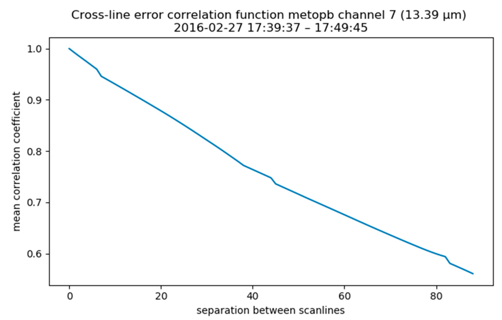
The matrices shown in Figure 2 and Figure 3 have not been averaged across the image to give a representative estimate. Since a significant part of their evident structure relates to variations in the pixel brightness temperature, it follows that the error correlation matrix is more stable, and, as described earlier, could be used in conjunction with the per-pixel uncertainty fields to estimate the error covariance for any given pair of pixels more precisely. However, it is not practical for a full orbit to include a cross-line error correlation matrix, and the further approximation using Equation (16) must be used. Figure 4 presents the cross-line error correlation function thus derived for the image of Figure 1, not just for pixel ‘A’, but sampled and averaged across the whole image.
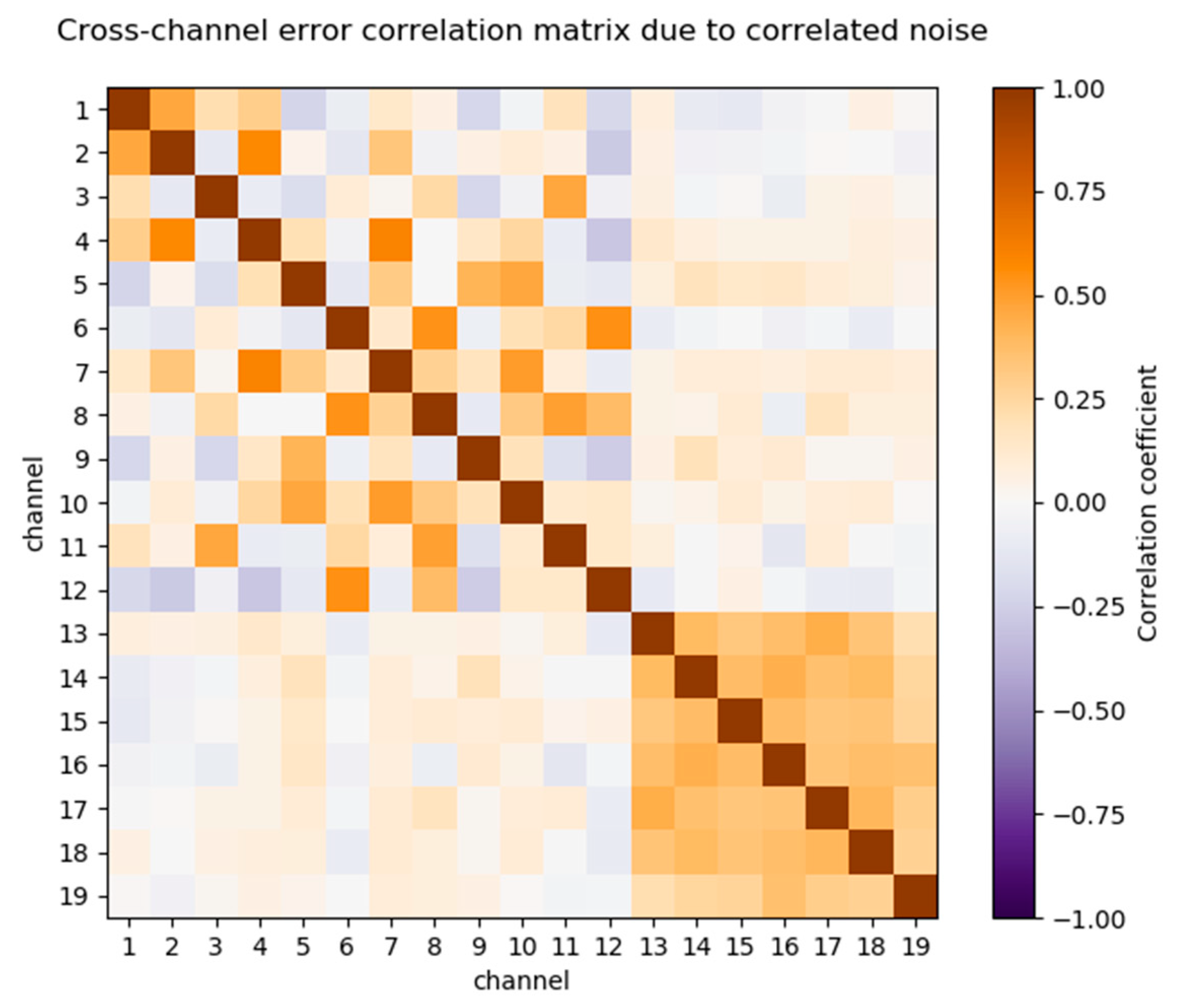
HIRS data are often used in multi-channel atmospheric sounding and for data assimilation, and so the cross-channel error correlations are important. Figure 5 shows an example obtained for the image in Figure 1. The matrix shows the error correlation between each pair of the 19 HIRS infra-red channels for independent effects. For this sensor, errors that are independent between pixels in an image (spatially) turn out to be partially correlated between channels, and so the off-diagonal terms of the cross-channel error correlation matrix are non-zero. There are two groups of channels that have cross-channel correlated noise between the channels in each group, but not between the groups, as can be seen from the block-diagonal form.
7. Conclusions
Uncertainty in derived climate data records and geophysical products comes in part from uncertainty in the satellite radiances used in the geophysical retrieval. Information about radiance uncertainty is generally not present in radiance products (level 1 data), compelling Earth observation practitioners doing geophysical retrievals to invent radiance uncertainty estimates or use other ad hoc methods to attribute uncertainties to results (if they do so at all). This situation falls short of best scientific and metrological practice, in which uncertainties at all stages are understood, characterised and propagated through to the final results. Although much useful science and many applications can be done without rigorous end-to-end treatment of uncertainty, where significant policy and liability questions rest on the integrity of observations, the trustworthiness and traceability of uncertainty estimates must be demonstrated.
However, providing uncertainty information at level 1 is not trivial. Radiance uncertainties are not simple. Uncertainty varies significantly from pixel-to-pixel, errors are correlated across the spatio-temporal domain in complex patterns that have their roots in instrument design and operation, and traditional consideration of “random vs. systematic errors” does not enable adequate characterisation of errors in satellite imagery. Moreover, solutions have to be practical for data producers and users, while still enabling a proper evaluation of uncertainty in derived products to be obtained. The full error covariance information for a multi-channel satellite image, even if we can estimate it, cannot be communicated to users because of the data volume implied.
This paper sets out one set of approaches that address the non-trivial aspects of providing users of radiance products with uncertainty information that is as simple as possible, but not simpler than necessary. Many details have inevitably been presented, so it is worth reviewing here the high-level concepts of the proposed solution.
First, the new uncertainty information available to users within a product following the methods presented here includes:
- Per-pixel, per-channel magnitude of radiance uncertainty
- Per-product, per-channel cross-element and cross-line radiance error correlation coefficients, and
- Per-product cross-channel radiance error correlation
Second, this uncertainty information is presented for a tri-partite classification of uncertainty components that adequately respects the complexity of errors in satellite imagery. The components describe the uncertainty that arises from errors that are independent (uncorrelated between pixels of a given channel), structured (patterned across an image) and common (systematic across a whole image).
Third, this set of uncertainty information gives users of radiance data a new capability to propagate uncertainty in a standardised, rigorous way through their retrieval process to derive uncertainty in their geophysical products. This includes where (i) the retrieval is multi-channel and therefore sensitive to any cross-channel correlations in errors, and (ii) where the target products aggregate in space and time and simplistic treatment radiance errors as “noise” would generally give under-estimates of uncertainty in the results. Propagation of the uncertainty information can be done using analytic or Monte Carlo methods [22].
Fourth, although some increase in data volume is necessary, it is minimised. (i) Uncertainty information need not be held to the same numerical precision as the radiances themselves, and so the per pixel provision of uncertainty information can be done such that the data volume is no more than doubled. (ii) Providing correlation functions as a function of pixel separation and the cross-channel error covariance matrices per radiance product has a small associated cost in data volume.
The framework presented above allows derivation of summary uncertainty (error covariance) information in radiance data based on systematic combination of instrumental error sources—a “bottom-up” approach. Is it reasonable to expect such an uncertainty analysis to become common practice? Space agencies already determine much of the necessary understanding of instrumental errors during instrument design, build and testing. Taking this instrument understanding forward into radiance uncertainty information for level-1 products, using the framework presented here or one similar, is therefore a value-adding extension of a much greater effort of characterisation that is already undertaken by agencies.
This work has been undertaken within the project Fidelity and Uncertainty in Climate data records from Earth Observation (FIDUCEO, www.fiduceo.eu), and the level 1 products being prepared at time of writing in that project have additional features, where relevant, to provide convenience to users. We will re-calibrate the satellite radiances to improve multi-sensor series. The products gather radiance, radiance uncertainty, viewing geometry and geolocation data in a self-described, compressed netCDF format. Lastly, at the scale of level-1 data collections, duplicate data are suppressed and orbits are consolidated. A standardised format for data across different sensor series allows tools to assist users with handling the uncertainty information to be designed, which will be the subject of a future paper.
Earth observation provides the largest and most globally descriptive set of information about the changing state of Earth’s environments. Proper interpretation of and inference from satellite data should be done in the context of well quantified uncertainties, to avoid wrong conclusions and bad decision-making. Practical delivery of the uncertainty information required presents a significant challenge and the methods in this paper are presented as candidate approaches to address this challenge.
Author Contributions
Conceptualisation, C.J.M., J.P.D.M. and E.R.W.; Funding acquisition, C.J.M. and J.P.D.M.; Methodology, C.J.M. and G.H.; Project administration, C.J.M.; Software, G.H.; Supervision, C.J.M. and J.P.D.M.; Visualisation, G.H.; Writing—original draft, C.J.M.; —review & editing, J.P.D.M., G.H. and E.R.W.
Funding
This research was performed within the project Fidelity and Uncertainty in Climate data records from Earth Observation (FIDUCEO, www.fiduceo.eu) which received funding from the European Union’s Horizon 2020 Programme for Research and Innovation, under Grant Agreement no. 638822.
Acknowledgments
Additional project administration was contributed by Rhona Phipps, University of Reading.
Conflicts of Interest
The authors declare no conflict of interest. The funders had no role in the design of the study; in the collection, analyses, or interpretation of data; in the writing of the manuscript, and in the decision to publish the results.
References
- Hollmann, R.; Merchant, C.J.; Saunders, R.; Downy, C.; Buchwitz, M.; Cazenave, A.; Chuvieco, E.; Defourny, P.; de Leeuw, G.; Forsberg, R.; et al. The ESA Climate Change Initiative: Satellite Data Records for Essential Climate Variables. Bull. Am. Meteorol. Soc. 2013, 1541–1552. [Google Scholar] [CrossRef]
- Plummer, S.; Lecomte, P.; Doherty, M. The ESA Climate Change Initiative (CCI): A European contribution to the generation of the Global Climate Observing System. Remote Sens. Environ. 2017, 203, 2–8. [Google Scholar] [CrossRef]
- Bates, J.J.; Privette, J.L.; Kearns, E.J.; Glance, W.; Zhao, X. Sustained Production of Multidecadal Climate Records: Lessons from the NOAA Climate Data Record Program. Bull. Am. Meteorol. Soc. 2015, 1573–1581. [Google Scholar] [CrossRef]
- Karlsson, K.-G.; Anttila, K.; Trentmann, J.; Stengel, M.; Fokke Meirink, J.; Devasthale, A.; Hanschmann, T.; Kothe, S.; Jääskeläinen, E.; Sedlar, J.; et al. CLARA-A2: The second edition of the CM SAF cloud and radiation data record from 34 years of global AVHRR data. Atmos. Chem. Phys. 2017, 5809–5828. [Google Scholar] [CrossRef]
- Notz, D. How well must climate models agree with observations? Phil. Trans. R. Soc. 2015, 373, 20140164. [Google Scholar] [CrossRef] [PubMed] [Green Version]
- Frigg, R.; Thompson, E.; Werndl, C. Philosophy of Climate Science Part 1: Observing Climate Change. Philos. Compass 2015, 10, 953–964. [Google Scholar] [CrossRef]
- Baumberger, C.; Knutti, R.; Hirsch Hadorn, G. Building confidence in climate model projections: An analysis of inferences from fit. Wiley Interdiscip. Rev. Clim. Chang. 2017, 8. [Google Scholar] [CrossRef]
- Bellprat, O.; Massonnet, F.; Siegert, S.; Prodhomme, C.; Macias-Gómez, D.; Guemas, V.; Doblas-Reyes, F. Uncertainty propagation in observational references to climate model scales. Remote Sens. Environ. 2015, 203, 101–108. [Google Scholar] [CrossRef]
- Zeng, Y.; Su, Z.; Calvet, J.-C.; Manninen, T.; Swinnen, E.; Schulz, J.; Roebeling, R.; Poli, P.; Tan, D.; Riihelä, A.; et al. Analysis of current validation practices in Europe for space-based climate data records of essential climate variables. Int. J. Appl. Earth Obs. Geoinf. 2015, 42, 150–161. [Google Scholar] [CrossRef]
- Su, Z.; Timmermans, W.; Zeng, Y.; Schulz, J.; John, V.O.; Roebeling, R.A.; Poli, P.; Tan, D.; Kaspar, F.; Kaiser-Weiss, A.; et al. An overview of European efforts in generating climate data records. Bull. Am. Meteorol. Soc. 2018, 99, 349–359. [Google Scholar] [CrossRef]
- Greenwald, T.; Bennartz, R.; Lebsock, M.; Teixeira, J. An Uncertainty Data Set for Passive Microwave Satellite Observations of Warm Cloud Liquid Water Path. J. Phys. Sci. Atmos. 2018, 123. [Google Scholar] [CrossRef] [PubMed]
- Ablain, M.; Cazenave, A.; Larnicol, G.; Balmaseda, M.; Cipollini, P.; Faugère, Y.; Fernandes, M.J.; Henry, O.; Johannessen, J.A.; Knudsen, P.; et al. Improved sea level record over the satellite altimetry era (1993–2010) from the Climate Change Initiative project. Ocean Sci. 2015, 11, 67–82. [Google Scholar] [CrossRef] [Green Version]
- Gruber, A.; Su, C.H.; Zwieback, S.; Crowd, W.; Dorigo, W.; Wagner, W. Recent advances in (soil moisture) triple collocation analysis. Int. J. Appl. Earth Obs. 2015, 45, 200–211. [Google Scholar] [CrossRef]
- Merchant, C.J.; Paul, F.; Popp, T.; Ablain, M.; Bontemps, S.; Defourny, P.; Hollmann, R.; Lavergne, P.; Laeng, A.; de Leeuw, G.; et al. Uncertainty information in climate data records from Earth observation. Earth Syst. Sci. Data 2017, 9, 511–527. [Google Scholar] [CrossRef] [Green Version]
- Mittaz, J.; Merchant, C.J.; Woolliams, E. Applying Principles of Metrology to Historical Earth Observations from Satellites. Metrologia 2019. under review. [Google Scholar]
- Quast, R.; Giering, R.; Govaerts, Y.; Rüthrich, F.; Roebeling, R. Climate Data Records from Meteosat First Generation Part II: Retrieval of the In-Flight Visible Spectral Response. Remote. Sens. 2019, 11, 480. [Google Scholar] [CrossRef]
- Govaerts, Y.; Rüthrich, F.; Viju, J.; Quast, R. Climate Data Records from Meteosat First Generation Part I: Simulation of Accurate Top-Of-Atmosphere Spectral Radiance over Pseudo-Invariant Calibration Sites for the Retrieval of the In-Flight VIS Spectral Response. Remote Sens. 2018, 10, 1959. [Google Scholar] [CrossRef]
- Holl, G.; Mittaz, J.P.D.; Merchant, C.J. Error covariances in High-resolution Infrared Radiation Sounder (HIRS) radiances. Remote Sens. 2019. under review. [Google Scholar]
- Hans, I.; Burgdorf, M.; Buehler, S.A.; John, V.O. An uncertainty quantified fundamental climate data record for microwave humidity sounders. Remote Sens. 2019. under review. [Google Scholar]
- Dee, D.P.; Uppala, S.M.; Simmons, A.J.; Berrisford, P.; Poli, P.; Kobayashi, S.; Andrae, U.; Balmaseda, M.A.; Balsamo, G.; Bauer, P.; Bechtold, P.; et al. The ERA-Interim reanalysis: Configuration and performance of the data assimilation system. Q. J. R. Meteorol. Soc. 2011, 137, 553–597. [Google Scholar] [CrossRef]
- Waller, J.A.; Dance, S.L.; Nichols, N.K. Theoretical insight into diagnosing observation error correlations using observation-minus-background and observation-minus-analysis statistics. Q. J. R. Meteorol. Soc. 2016, 142, 418–431. [Google Scholar] [CrossRef]
- Joint Committee for Guides in Metrology: Evaluation of Measurement Data—Guide to the Expression of Uncertainty in Measurement. 2008. Available online: https://www.bipm.org/utils/common/documents/jcgm/JCGM_100_2008_E.pdf (accessed on 12 December 2018).
- Bulgin, C.; Embury, O.; Merchant, C.J. Sampling uncertainty in gridded sea surface temperature products and Advanced Very High Resolution Radiometer (AVHRR) Global Area Coverage (GAC) data. Remote Sens. Environ. 2016, 177, 287–294. [Google Scholar] [CrossRef]
- Datla, R.U.; Rice, J.P.; Lykke, K.R.; Johnson, B.C.; Butler, J.J.; Xiong, X. Best Practice Guidelines for Pre-Launch Characterization and Calibration of Instruments for Passive Optical Remote Sensing. J. Res. Natl. Inst. Stand. Technol. 2011, 116, 621–646. [Google Scholar] [CrossRef] [PubMed]
- Hans, I.; Burgdorf, M.; John, V.O.; Mittaz, J.; Buehler, S.A. Noise performance of microwave humidity sounders over their lifetime. Atmos. Meas. Tech. 2017, 10, 4927–4945. [Google Scholar] [CrossRef] [Green Version]
- Desmons, M.; Mittaz, J.; Taylor, M.; Merchant, C.J. Instrumental noise in the visible and infrared channels of the AVHRR. Remote. Sens. 2019. in preparation. [Google Scholar]
- Smith, D.L.; Delderfield, J.; Drummond, D.; Edwards, T.; Mutlow, C.T.; Read, P.D.; Toplis, G.M. Calibration of the AATSR Instrument. Adv. Space Res. 2001, 28. [Google Scholar] [CrossRef]
- Walton, C.C.; Sullivan, J.T.; Rao, C.R.N.; Weinreb, M.P. Corrections for detector nonlinearities and calibration inconsistencies for the infrared channels of the Advanced Very High Resolution Radiometer. J. Geophys. Res. 1998, 103, 3323–3357. [Google Scholar] [CrossRef]
- Christy, J.R.; Spencer, R.W.; Braswell, W.D. MSU tropospheric temperatures: Dataset construction and radiosonde comparisons. J. Atmos. Ocean. Technol. 2000, 17, 1153–1170. [Google Scholar] [CrossRef]
- Dudhia, A. Noise characteristics of the AVHRR infrared channels. Int. J. Remote Sens. 2007, 10, 637–644. [Google Scholar] [CrossRef]
- Coppersmith, D.; Winograd, S. Matrix multiplication via arithmetic progressions. J. Symb. Comput. 1990, 9. [Google Scholar] [CrossRef]
- Oliphant, T.E. A Guide to NumPy; Trelgol Publishing: Spanish Fork, UT, USA, 2006. [Google Scholar]
- Koenig, E.W. Final Report on the High Resolution Infrared Radiation Sounder (HIRS) for the Nimbus F Spacecraft, ITT Aerospace/Optical Division. 1975. Available online: https://ntrs.nasa.gov/archive/nasa/casi.ntrs.nasa.gov/19760014184.pdf (accessed on 1 October 2018).
- Shi, L.; Bates, J.J. Three decades of intersatellite-calibrated High-Resolution Infrared Radiation Sounder upper tropospheric water vapor. J. Geophys. Res. 2011, 116. [Google Scholar] [CrossRef] [Green Version]
Figure 1.
Top left: Brightness temperature image raster of an extract between 17:39:73 and 17:49:51 UTC of HIRS channel 7 on Metop-A. Top right, and lower row: the corresponding fields of standard uncertainty in brightness temperature arising from independent, structured and common errors. The red square labelled ‘A’ indicates a specific pixel and the dashed lines the position of the scan and element arrays through ‘A’. The imagery is taken from a descending pass.

Figure 2.
Cross-element error covariance matrix calculated for the scan line through point ‘A’ of Figure 1. HIRS scans such that element indices 0 to 55 run from east to west (right to left) in Figure 1. The range of the colour scale corresponds to brightness temperature uncertainty from 0.10 K to 0.13 K. The matrix shown gives the error covariance from structured effects.

Figure 3.
Cross-line error covariance matrix calculated for the line of constant element number through point ‘A’ of Figure 1. Since this is a descending pass of the satellite, the scanline indices 0 to 88 run from north to south (top to bottom) in Figure 1. The range of the colour scale corresponds to brightness temperature uncertainty from 0.06 K to 0.13 K. The matrix shown gives the error covariance from structured effects.

Figure 4.
Cross-line error correlation function representative of error correlations from structured effects for the data in Figure 1.
Figure 4.
Cross-line error correlation function representative of error correlations from structured effects for the data in Figure 1.

Figure 5.
Cross-channel error correlation matrix, , from spatially independent effects, corresponding to data in Figure 1.
Figure 5.
Cross-channel error correlation matrix, , from spatially independent effects, corresponding to data in Figure 1.

© 2019 by the authors. Licensee MDPI, Basel, Switzerland. This article is an open access article distributed under the terms and conditions of the Creative Commons Attribution (CC BY) license (http://creativecommons.org/licenses/by/4.0/).
Share and Cite
MDPI and ACS Style
Merchant, C.J.; Holl, G.; Mittaz, J.P.D.; Woolliams, E.R. Radiance Uncertainty Characterisation to Facilitate Climate Data Record Creation. Remote Sens. 2019, 11, 474. https://doi.org/10.3390/rs11050474
AMA Style
Merchant CJ, Holl G, Mittaz JPD, Woolliams ER. Radiance Uncertainty Characterisation to Facilitate Climate Data Record Creation. Remote Sensing. 2019; 11(5):474. https://doi.org/10.3390/rs11050474
Chicago/Turabian StyleMerchant, Christopher J., Gerrit Holl, Jonathan P. D. Mittaz, and Emma R. Woolliams. 2019. "Radiance Uncertainty Characterisation to Facilitate Climate Data Record Creation" Remote Sensing 11, no. 5: 474. https://doi.org/10.3390/rs11050474
Note that from the first issue of 2016, this journal uses article numbers instead of page numbers. See further details here.